

Submitted:
18 July 2026
Posted:
20 July 2026
You are already at the latest version
Abstract
The physical environment of a neighborhood and its ambient population density appears to be closely related, but this relationship is difficult to measure quantitatively. A previous study addressed this challenge by developing a baseline machine learning model capable of estimating Average Hourly Ambient Population Density (AHAPD) from neighborhood physical environment features, achieving 75.9% accuracy. This study compares the performance of the baseline model with collective human intuition and AI models in estimating AHAPD at the neighborhood level. A 29-section questionnaire was used to evaluate the performance of the three respondent types across three metrics: accuracy, reasoning, and confidence. In total, 100 response sets were analysed, comprising 94 human responses, five responses from vision-capable AI models, and one output from the previously trained XGBoost baseline model. The results show that the ML baseline model, trained on a relatively small dataset using 16 input features, outperformed the average human score and the average score of five selected commercially available AI models, while achieving accuracy comparable to the average human with domain expertise. The study concludes with case studies and discussion of differences in reasoning behavior, confidence levels, and the strengths and weaknesses of each respondent type.
Keywords:
neighborhood planning
; machine learning
; comparative study
; ambient population density
; GIS
; AI
1. Introduction
The physical environment of a neighborhood, while indirect, appears to be closely related to its ambient population density [1,2,3,4,5]. However, quantitatively measuring this relationship is challenging, as the physical environment consists of many interrelated features, and an accurate representation of ambient population density is difficult to obtain. In a previous study by Rojradtanasiri et al. [6], an alternative method for estimating ambient population density, a spatial population density that accounts for daytime movement habits [2], at the neighborhood scale was explored. The study used physical environment features collected using Geographic Information System (GIS) [7], OpenStreetMap (OSM) database [8], and basic statistics as inputs. These inputs were paired with the average hourly Mobile Spatial Statistics (MSS) [9] data available in Japan [10], which were used as a representation of ambient population density, to create neighborhood profiles. In total, 900 neighborhood profiles from across Japan were compiled and used as the dataset for training Machine Learning (ML) models [11]. The objective was to classify neighborhoods into categories based on their Average Hourly Ambient Population Density (AHAPD).
The result was a trained XGBoost model [12] that used 16 input features, including physical environment features from OSM, a globally available open-source dataset, and basic statistical data collected from e-Stat [13]. The model successfully classified neighborhoods into three AHAPD classes with an accuracy (F1 score [14]) of 75.9%. Feature Importance was analyzed using SHapley Additive exPlanations (SHAP) [15] and Partial Dependence Plots (PDP) [16]. Although the dataset size was relatively small compared to state-of-the-art AI models trained on massive datasets [17,18], the results demonstrated acceptable accuracy and provided strong evidence of a relationship between physical environment and AHAPD, serving as a proof of concept.
Findings from the study include the top three most influential input features for neighborhoods with high AHAPD were LandUseDiversity, BasedDensity, and RoadCount [6]. The identification of threshold values where the correlation between specific features and ambient population density changed from positive to negative; this finding points to new areas for investigation. The overall, by-class and predictive-instance feature importance scores provide insights into how models make each decision, or the reasoning. Additionally, the model’s confidence scores for each predictive instance reveal insights about the model’s confidence level and correctness of the prediction, which are also valuable. These metrics (accuracy, reasoning, and confidence) form the foundation for evaluating model performance.
While an F1 score of 75.9% appears relatively high, it is difficult to assess whether this level of accuracy is satisfactory without a comparison with other types of evaluator, such as performance comparison with human intuition or vision-capable AI models. This leads to the main objective of this study: to evaluate the previously trained baseline model’s performance on estimating AHAPD and to better understand its behavior.
Comparing ML models performance against humans or other models is a common practice across many domains. The tasks that typically get compared generally fall into two categories: (1) tasks that can be evaluated using existing standardized tests as a benchmark, and (2) specialized tasks without a standardized test. Examples of the first category include evaluating a newly released AI models using benchmarks like AIME [19], a dataset containing competition math problems, to assess mathematical ability; Humanity’s Last Exam (HLE) [20], a dataset of over 2,500 challenging questions from over hundred subjects, to evaluate expert level knowledge and reasoning; standardized Physics Olympiad problems [21], to evaluate capability in physics; the IEEExtreme coding challenge [22] to evaluate coding skills; and the Bar Exam [23] to evaluate knowledge in law. These benchmarks provide common, comparable metrics for demonstrating model capability. Because AI models are versatile, they can be adapted to existing benchmarks with historical human performance records, so using standardized benchmarks is often preferable.
For the second category (specialized tasks without a standardized test), new customized tests need to be developed as a benchmark to fairly evaluate each model. This category is suitable for ML models that are less versatile, have limited capability, and were trained to perform only specific tasks. For example, Jammal et al. [24] compared a deep learning model with two glaucoma specialists by presenting them with 490 fundus images for grading. Similarly, Salinas et al. [25] reviewed 53 studies that compared AI (Artificial Intelligence) performance with dermatologists for skin cancer classification. Shehu et al. [26] assessed emotion detection from facial expressions by comparing the judgments of 82 humans and ML classifiers. In all these examples, past human performance data was not available. The models were first trained and then later compared with humans. Therefore, new evaluation tools, such as expert-reviewed datasets or controlled questionnaires, had to be developed to ensure a fair comparison.
In our case, the baseline ML model was trained for a niche task of estimating AHAPD, which has no standardized test (category 2); therefore, a new customized test is needed. The key to designing a new benchmark is fairness [27], ensuring that none of the participant types has an unfair advantage. For instance, the same set of information, such as the 16 features that the baseline model uses as its main basis for prediction, is also given to human participants and AI models. However, in our case it is very challenging to replicate the test at exactly 1:1, because each participant type has different strengths and weaknesses. For example, the baseline model has been trained on the AHAPD data and can interpret numbers well, but it has no vision capability. Humans have visual and experience advantages but may have limited capability in finding patterns within raw numerical values. AI models, on the other hand, have the advantage of being trained on large scale dataset, are vision capable, and can interpret numbers very well, but face rate limits [28], have limited context windows [29] and memory [30], and sometimes hallucinate [31]. These strengths and weaknesses must be considered when designing the benchmark.
Another important factor to consider is balancing the complexity and accessibility of the benchmark. A complex benchmark that requires time, effort, and specialized skill will limit participation to only a few specialists. For example, tasks requiring expert knowledge, such as glaucoma detection, may involve only two trained specialists. In contrast, a simpler, shorter benchmark is more suitable for the general public and can involve a larger number of participants. A more general task like emotion recognition can be evaluated by a larger pool of participants (e.g., 82 participants in Shehu et al. [26]). Estimating AHAPD lies closer to a general task than a complex one.
Although there is no official training for this specific task, there are human specialist conducted studies focusing on distinguishing urban from rural areas which require similar skills. For example, Sarmadi et al. [32] compared the performance of convolutional neural networks (CNNs) [33] with 102 human experts in estimating poverty from aerial images. While the CNN outperformed the experts, the score and features identified by the experts were used for training the model. Ahn et al. [34] used a human-machine collaborative approach to estimate regional economic development from satellite imagery, in which human annotators were asked to label clusters of images for training supervised deep learning models. Panczak et al. [35] conducted a literature review of temporal population estimation methods and identified 96 relevant studies. These studies suggest that this is an active area of research and that human judgment is often relied upon. Similarly, professionals in architecture, urban design, and real estate development may have an intuitive edge in this type of visual-spatial recognition, as they are more familiar with maps, aerial images, and urban elements. Therefore, to identify where the baseline model stands relative to other groups, it is meaningful to compare people with and without such domain expertise, highlighting the need for the benchmark to be accessible to a diverse group.
Another advantage of applying AI models like ChatGPT [36] on existing tests is that they can be used as objective tools to evaluate test difficulty. For example, Suresh and Rawat [37], used ChatGPT to assess the difficulty of SAT exams [38] and re-evaluate past human performance. Similarly, the confidence score of the pre-trained baseline model can be used as an objective measure of the difficulty level of each question in the benchmark, which can help assess the strength and weakness of each participant type.
In conclusion, this study focuses on comparing the performance of a previously trained baseline model with humans and AI models on the task of estimating AHAPD, which has no existing standardized test. A novel questionnaire-based benchmark was created to fairly evaluate each participant type across three dimensions: accuracy, reasoning, and confidence. The study had two primary goals: (1) to evaluate the baseline model’s performance and assess its potential as a practical tool. (2) to analyze and gain insights into the strengths, weaknesses, similarities and differences in decision-making processes of each participant type. Finally, this study highlights the strengths and limitations of both machine and human predictions, offering a deeper understanding of how ML models reason and how they compare with human intuitive judgment.
2. Methodology
To compare the performance of our baseline model with human intuition and vision-capable AI models, we created a questionnaire based benchmarking tool using Google Forms [39], designed to fairly evaluate the three aspects: accuracy, confidence, and reasoning. The comparison does not test the three respondent types under identical input conditions. Instead, it compares each respondent type under realistic conditions suited to its mode of judgment: numerical feature values for the baseline model, and visual-numerical questionnaire materials for humans and AI models. All participants were informed about the purpose of the research, that participation was voluntary, and that their data would be anonymized and used only for academic purposes. Consent to participate was collected electronically before the questionnaire began.
Early versions of this questionnaire were tested with a group of peers and colleagues from the same university cohort for feedback. Multiple iterations were developed and tested before external distribution. The response period was set until 100 responses were received. All responses were analyzed and discussed before drawing conclusions. An overview of this process is shown in Figure 1, with details explained in the following sections.
2.1. Compliance with Ethical Standards
All research involving human participants was performed in accordance with the principles stated in the Declaration of Helsinki. Formal ethical approval from a local Institutional Review Board (IRB) or equivalent ethics committee was not sought for this study. The reason is that the research involved an online survey in a non-medical field, which is classified as minimal risk. Informed consent was obtained from all participants before they could access and begin the questionnaire. No personal information was required. The ‘Name’ field was optional and was used to track submission status only. All data used for analysis were fully anonymized and could not be linked back to individual respondents. The data collected were used exclusively for academic research.
2.2. Questionnaire Design
To evaluate accuracy, confidence, and reasoning, we used common questionnaire tools. Classification accuracy was assessed with multiple-choice questions. Reasoning was evaluated by asking respondents to select 5 of 16 given features they believed most influenced their decision. Confidence was measured by having respondents rate their certainty on a scale of 1 to 10.
The first version of the questionnaire included 20 sections, each with three in-depth questions. Early feedback indicated that the questionnaire was too long, overly technical, and difficult to complete, even among those with domain expertise. Respondents reported that reasoning-type questions were particularly time-consuming and difficult, especially in the pre-questionnaire section where no examples were provided before answering. Some early testers without domain expertise reported struggling with domain-specific terms such as “neighborhood”, “features” and “traffic”. Several also noted that without a training section it was difficult to complete the questionnaire because there was no feedback or chance to recalibrate their responses. Additionally, respondents were curious to know their scores after completing, which were not shown in the first version.
In response, we simplified the language, reduced the number of reasoning questions, made some questions optional, and introduced a training section where respondents could check the accuracy of their first three answers and recalibrate their decisions. A final score display was also added to satisfy participant curiosity about their performance. The final version of the questionnaire consisted of four sections: Basic Information, Training, Main Questionnaire, and Post-Questionnaire. Each section is explained in detail below.
2.2.1. Basic Information
This section consists of 7 questions to collect respondents’ demographics: Name (optional), Age, Nationality, Country of Residence, Occupation, and Experience in Japan (in years). Initially, names were excluded, but later were added (as optional) to track which invitee has already submitted their response. These questions were intended to capture respondent’s experience, familiarity to Japan, and their level of domain expertise, since these factors may influence their performance and reasoning.
The seventh question (optional) asked respondents to select 5 of 16 features they believed most influenced the ambient population density of a neighborhood. This question was intended to capture respondents’ overall preconceptions and was planned to be compared with their selections in the post-questionnaire section.
2.2.2. Training
The training section included 3 sets of questions (S1-S3), each with three questions (Q1-Q3).
- Q1: a multiple-choice classification question aiming to evaluate accuracy, asking respondents to select A, B or C (A = Class 0, B = Class 1, C = Class 2), based on an aerial image and a bar chart showing the value of 16 features associated with the neighborhood.
- Q2: a multi-select question to evaluate reasoning, asking respondents to choose 5 of 16 features that most influenced their decision.
- Q3: a rating question asking respondents to rate their confidence on a scale of 1 to 10. The results are used to identify which questions respondents found easier or harder.
For the training questions, we chose one example from each class in which the model made a correct prediction with high confidence, representing easier questions (Table 1). After completing the three sets, the correct answers were shown, allowing respondents to recalibrate their decisions. Figure 2 shows an example of the three question types used in the questionnaire.
2.2.3. Main Questionnaire
This section contained 26 sets of questions (S4-S29), following the same structure as the training section but without immediate feedback. The first 23 sets (S4-S26) included only Q1 (Accuracy) and Q3 (Confidence), to reduce time requirements and complexity. The last 3 sets (S27-S29) included Q2 (Reasoning). Because the first appearance of the reasoning item in the main flow was optional, we prioritized these end-of-survey reasoning questions.
Neighborhoods used in each set were selected from the prediction that baseline model made using testing dataset. This selection was intended to create a diagnostic questionnaire benchmark for comparing respondent behavior across different levels of model confidence and correctness, rather than replicating the baseline model’s overall performance on the full test dataset. The full list of predictions were extracted from the confusion matrix [40] (Figure A1) and reorganized based on the prediction confidence and correctness. Questions that the baseline model answered correctly with high confidence were classified as Easy. Questions where the model had low confidence were classified as Medium. Questions the model answered incorrectly with high confidence were classified as Hard. The final 26 questions consisted of 6 Easy, 7 Medium, and 13 Hard. Of these, the baseline model correctly answered 13 and failed 13, representing a 50 percent accuracy baseline. Respondents needed to score above 16 points (including the training questions) to outperform the model.
2.2.4. Post-Questionnaire
This section consisted of 6 reflective questions, asking respondents to rate their overall confidence and explain their reasoning when choosing A, B or C in free-form text format. This was intended to capture reasoning that may not be fully captured by the multi-selection Q2 questions. For one last time, respondents were asked to select the 5 most influential features for their overall reasoning. The final question asked respondents for any final comments on the questionnaire (optional).
2.3. Evaluating Accuracy, Reasoning, and Confidence
Table 2 summarizes which questionnaire items were used to evaluate each metric and where they appear in the questionnaire structure. After collecting all responses, the raw answers were processed to calculate the final Accuracy, Reasoning and Confidence score. Details on how each score was calculated are shown in next sections.
2.3.1. Accuracy—Multiple Choice (Q1)
The calculation of the final accuracy scores is straightforward. The raw data were evaluated using several statistics, such as mean, minimum, maximum, median, and mode, across all respondents and demographic subgroups. This analysis helped identify behavioral patterns and allowed performance comparison between respondent types.
2.3.2. Reasoning—Select 5 Features (Q2)
By analyzing the baseline model using SHAP, feature importance scores can be extracted for each context (), either overall or class-specific (Classes 0, 1 or 2). These scores measure the contribution of each feature to the model’s prediction and are used as the baseline representing model reasoning.
To capture human- and AI-perceived feature importance, respondents were asked to select 5 of the 16 features in up to eight instances: four at the beginning of the questionnaire (optional) and four at the end. Each set of four selections corresponded to one overall feature importance context () and three class-specific contexts ( for Class 0, for Class 1, and for Class 2). Because the initial selections were optional and may be incomplete, only the four end-of-questionnaire selections were used in the analysis.
For each context , each respondent distributed a total score of 1 equally among their 5 selected features, giving each selected feature a weight of . Let be the number of respondents, and let indicate whether respondence selected features in context ( = 1 if selected, 0 otherwise). The Derived Feature Importance () for features in context is calculated as:
where:
is the total number of respondents.
represent an individual respondent.
represents the evaluation context (overall, Class 0, Class 1, or Class 2)
represents one of the 16 input features.
equals 1 if respondent selected feature in context , and 0 otherwise.
This score represents the average feature importance assigned to each feature across all respondents within a given context. This metric enables direct comparison between human, AI, and baseline model perceived feature importance, allowing similarities and differences in reasoning to be identified across all respondents types and contexts.
2.3.3. Confidence—Rating (Q3)
Model confidence scores were used to classify question difficulty and analyze the behavior of the baseline model. Human confidence level was collected using rating-type questions. However, raw confidence scores may vary across respondents due to personality differences (e.g., conservative versus bold respondents). To reduce this variation, each respondent’s confidence scores were normalized based on their personal range.
For each respondent , the minimum ( and maximum () confidence scores across all questions were identified. For a given question (), the normalized confidence score is calculated as:
where is the raw confidence score provided by respondent for question . This normalization scales each respondent’s confidence scores to a range between 0 and 1, with their minimum confidence mapped to 0 and maximum confidence mapped to 1.
The Average Confidence for question () is then calculated as:
where:
is the total number of respondents.
is the raw confidence score provided by respondent for question .
and are the minimum and maximum confidence scores reported by respondent , respectively.
This metric represents the average normalized confidence of all respondents for a given question. Higher values indicate that respondents collectively found a question easier, whereas lower values indicate that it was perceived as more difficult. Human--derived values were compared with the baseline model’s confidence scores to identify similarities and discrepancies, including instances where predictions were confidently correct or confidently incorrect. AI models, was calculated using the same procedure as for human respondents.
2.4. Questionnaire Distribution
The questionnaire was distributed in two phases: Internal (early tester), intended to collect feedback and refine the questionnaire. External (invitation-only), targeting a diverse group of peers, colleagues, and family members. For participants unfamiliar with online forms, one-on-one support was provided via online meetings. The author presented the questions, translated where necessary, and submitted answers on their behalf with minimal interference to preserve objectivity.
For AI models, the questionnaire was submitted as images to five vision-capable models: GPT-4o [41], GPT-5 [42], Gemini 2.5 Flash [43], Claude Sonnet 4 [44], and Grok-3 [45], on August 21, 2025. These five models represented the leading commercially available AI models at the time the study was conducted. The free version of each model was used to participate in the questionnaire. Screen-captured images of each questionnaire page were saved in .jpeg format and submitted to each AI model one image at a time, in the same sequence, within a single chat session. For models where the rate limit was reached, we waited until the cool down period ended before submitting the remaining images in the same chat. The conversation with each model was started with the following identical prompt to maintain consistency.
“Today, I would like you to participate in my research by answering a set of questionnaires. I will provide you with screenshots of the questions, and you should respond with how you personally would answer them. I will then input your answers into the questionnaire on your behalf. Please do not look up the answers on the internet. Simply answer based on your own knowledge, experience, or opinion.”
Their responses were then manually entered by the author into the same Google Form that was distributed to other respondents. The AI model results were recorded and analyzed alongside human results.
3. Results
In total, it took 107 days, from 8 June to 22 September 2025, to receive all 100 responses. Responses from one minor and early testers were excluded from the analysis. The final response sets used for analysis consisted of 94 human responses, 5 AI model responses, and 1 output from the baseline model. Among human respondents ages range from 18 to 78, with an average of 35. The top nationalities by percentage were Thai (41.5%), Japanese (26.6%), Chinese (9.6%), and others (22.3%), which included American, Austrian, Australian, Bhutanese, French, Irish, Italian, Indian, Macedonian, Singaporean, and more. Of the human respondents, 59.5% had experience living in Japan (34.0% lived in Japan; 25.5% were native Japanese) and 40.5% had no experience living in Japan (9.6% had never been to Japan; 30.9% had visited only as tourists).
There were 41 unique professions among respondents, with the largest group being university students (29.8%) , followed by architects (9.6%); the remaining 60.6% were a combination of other professions such as banker, investor, animator, engineer, designer, marketer, and more. Among these 36 professions, roles such as architects, engineers, real estate agents, landscape designers are considered to have domain expertise, because the nature of their work may make them more familiar with maps, urban planning, and technical terms used in the questionnaire. Similarly, roles such as sales, business managers, and bankers are considered without domain expertise. Overall, 47.9% of human respondents were from professions with domain expertise and 52.1% were from professions without domain expertise. AI models and the baseline model are reported as separate categories and are excluded from the human domain expertise counts. Table 3 summarizes the demographic of our respondents and their average scores.
3.1. Accuracy Score
The average score across all respondents was 15.1 (training questions included), with a range of 9 to 22 points (Table 3). 33 percent of human respondents outperformed the baseline model (s=16), and 67% scored less than or equal to the baseline (Figure 3). Domain expertise appears to be an indicator associated with the performance (Figure 4). Within the same subgroup, those with domain expertise outperformed those without by an average of 1.3 points. Experience in Japan showed mixed results among those with domain expertise. The best-performing subgroups were those who had visited Japan as a tourist with domain expertise, however, this may be due to the small sample size in this subgroup (n=4). Among those without domain expertise, the highest average score was from respondents who had never been to Japan, although this group was also very small (n=2). The AI models scored between 10 and 18 points, with an average of 14.2 points, similar to the average of respondents without domain expertise.
The highest recorded human score exceeded the baseline by 37.5%, while the baseline exceeded the lowest recorded human score by 77.8%. These results indicate that the baseline performs at a similar level to the average respondent with domain expertise and outperforms the average of those without domain expertise by 10.3%.
3.2. Reasoning Score
We use feature importance scores derived from SHAP as a baseline to compare reasoning for each respondent type. By analyzing these scores, we can measure the strength of impact of each feature. Figure 5 shows the feature importance scores for each respondent type across all four contexts (overall, Class 0, 1 and 2). The features are arranged in descending order based on human-perceived impact. By comparing differences in these scores across respondent types, we can identify similarities and differences in their way of reasoning. Table 4 highlights the five features with the largest differences between humans and the baseline model, and also shows the differences between humans and AI models for those features.
From Figure 5, the features that most frequently appear in the top five across respondent types and contexts are RoadCount, LandUseDiversity, ResidentialA, CommercialA, and TransportationA. TaxIncome is the most divisive feature, appearing in the baseline model’s top five but not in the others. Humans and the baseline model agree on the importance of LandUseDiversity and TotalLandUse, whereas AI models do not. Humans and AI models agree that ResidentialA, TransportationA, and CommercialA are most influential, but the baseline model does not. The most frequent top five appearances are ResidentialA for humans, TransportationA for AI models, and RoadCount for the baseline model. The detailed explanation of each input feature, how they were calculated, and their SHAP values are shown in Table A2.
Another behavioral pattern that can be identified is the allocation of importance. Human selections are spread more evenly across features, forming a gradual distribution. AI models selections are more concentrated on only a few features (this could be due to the limited number of AI models respondents). In contrast, the baseline model places more weight on a small set of features in all contexts and assigns very light weight to others. In addition, the weight ranking varies less across contexts for humans and AI models, but changes significantly for the baseline model.
Table 4 lists the five features with the largest weight differences between humans and the baseline model for each context. Overall, both RoadCount and LandUseDiversity appear in the top five for humans and the baseline model. However, their assigned importance differs significantly: +16.49 percentage points for RoadCount and +9.91 for LandUseDiversity, indicating that the baseline model considers these features more significant than humans do. In contrast, ResidentialA and TransportationA show differences of -9.85 and -6.56 percentage points, indicating that humans view these features as more influential than the baseline model does. These gaps reflect different ways of reasoning between humans and the baseline. For the same set of features, the differences between AI models and humans are smaller than those between humans and the baseline model, indicating closer alignment in reasoning between humans and AI models.
3.3. Confidence Score
Figure 6 shows the respondents’ confidence scores for every question in the questionnaire, along with the correctness of their decisions. Answers in the green box indicate correct responses. The blue vertical dotted line divides the training questions from the main questionnaire. By examining this figure a few insights can be extracted. First, on average 72 percent of human respondents answered the training questions correctly even without prior training. The question most frequently answered correctly by humans was S29Q1 (Kurobe-Unazukionsen, Toyama), with an 89 percent correct rate, while the question with the fewest correct answers was S16Q1 (Hino, Shiga), with only five humans answering correctly, and both the baseline and AI models were also wrong.
Looking more closely at the confidence level and correctness, several behavior patterns emerge. There are cases where the model is both correct and highly confident, as in S1Q1 (Iwatenumakunai, Iwate), where it was 99 percent confident that the answer is Class 0, and it is correct. There are also cases where the model made right (S29Q1: Kurobe-Unazukionsen, Toyama) and wrong (S23Q1: Fukaya, Saitama) predictions with low confidence. However, discrepancies appear in S11Q1 (Sakurahommachi, Gifu), where the model was 98 percent confident in Class 1 but wrong, and in S12Q1 (Sasabaru, Fukuoka), where it predicted Class 0 while the correct answer was Class 2, the opposite end of the spectrum.
In contrast, for humans there is no instance of an incorrect decision made with high confidence, their confidence levels are correlated with the correctness. For S21Q1 (Yasu, Kochi), where most humans were wrong, the collective confidence was only 19 percent, and 80 percent answered incorrectly. For 29Q1 (Kurobe-Unazukionsen), where 89 percent answered correctly, the collective confidence was also 89 percent. A similar pattern appears for AI models. Questions with average confidence above 60 percent were usually answered correctly. For example, in S7Q1 (Nahari, Kochi), all five AI models are 100 percent confident and all were correct; in S19Q1 (Kashiwa, Chiba) all five AI models were wrong with confidence near 0.
These observations, together with the confidence scores for each respondent group, provide insight into predictive behavior and indicate which questions each group found easier or harder. Figure 6 also shows the aerial images and associated parameter values for several of the questions mentioned. These behavioral findings are discussed further in the discussion section.
4. Discussion
From the results, domain expertise appears to be one of the factors associated with better performance. Those with domain expertise outperformed those without by an average of 1.3 points across all subgroups. Being a native Japanese respondent shows an advantage among those without domain expertise but makes little difference among those with domain expertise. While unequal subgroup sizes may partly explain this pattern, a plausible reason is that non-experts find it harder to extract cues from the provided information, whereas native Japanese respondents may recognize neighborhoods from their names, giving them an advantage. Conversely, among respondents with domain expertise, prior contextual knowledge may introduce bias that leads to errors. On the other hand, those unfamiliar with Japanese neighborhoods may rely more objectively on the given aerial images and the values of each parameter, sometimes resulting in higher scores.
During the feedback session, many reported that they found the questionnaire challenging, even among those with domain expertise, especially during the training section, since it was their first exposure to this task. Yet, 72 percent of the respondents answered the training questions correctly. Both performance and speed increased after the training section, even as the difficulty gradually increased. Because of this on-the-spot learning, the last question, S29Q1, was the question most humans answered correctly.
For AI model performance, we initially expected strong results given their extensive pre-training with a large amount of dataset. In practice, only two out of five tested models outperformed the baseline model. Possible reasons include the uniqueness of the dataset used to train the baseline model, which AI models have not seen, rate limits during the questionnaire session, prompt fatigue from repeated similar inputs, and limited context windows. Early questions often received careful, accurate AI models responses, but with repeated prompts some models began to assume inputs were identical and invested less effort in image analysis. Limited memory also prevented AI models from retaining their earlier answers, so they could not learn across items, unlike humans. While humans improved with experience, AI model performance sometimes declined over time.
Regarding reasoning, we see more similarity between humans and AI models, than between humans and the baseline model. The differences appear in the weight assigned to each parameter (Table 4). The baseline model assigns more weight to RoadCount and LandUseDiversity, humans give more weight to ResidentialA and CommercialA, and AI models give the most weight to TransportationA. These differences may be due to the differences in the inputs. The baseline model depends solely on numerical values, whereas humans and AI models may rely more on visual cues. Therefore, parameters that are easily recognized from aerial images, such as ResidentialA, CommercialA and GreenA, may seem more influential. While it is not obvious which reasoning is superior, these differences provide useful insights by offering a second opinion, sometimes counterintuitive, which may lead to meaningful findings.
From a confidence perspective, humans and AI models also shared similar behavior, whereas the baseline model differed. Humans’ and AI models’ confidence scores correlate with the correctness of their answers, while the baseline model sometimes shows discrepancies, such as in S11Q1, where it was 98 percent confident but wrong. The questions each group found difficult, as indicated by confidence, also differ. For instance, in S29Q1 the baseline model had low confidence, yet most humans answered correctly with high confidence. In contrast, for S21Q1 the baseline model was very confident and correct, whereas humans and AI models reported very low confidence. This similarity between humans and AI models may reflect that AI models are trained on human generated data and can inherit human-like behavior, whereas the baseline model was trained solely on the specific dataset and does not inherit such characteristics.
Another notable characteristic is the difference in prediction patterns between humans, AI models, and the baseline model. Human and AI predictions generally reflect gradual changes, with predictions tending to progress from Class 0 to Class 1 and then to Class 2. In contrast, the baseline model does not always follow this pattern. Although rare, it occasionally makes predictions from Class 0 to Class 2, or vice versa. One example is S12Q1 (Sasabaru, Fukuoka), where the baseline model predicted Class 0 even though the correct answer was Class 2. This behavior suggests that the baseline model sometimes relies on counterintuitive reasoning that differs from human intuition.
4.1. Case Studies
The question most frequently answered correctly was S29Q1 (Kurobe-Unazukionsen, Toyama), a Class 0 neighborhood that the baseline model also predicted correctly, although with low confidence (0.56). The aerial image shows low building density and farmlands, which are clear indicators of Class 0. These features are easy to recognize, and the fact that it was the last question likely helped, since respondents could draw on experience from earlier questions. However, on closer inspection, this neighborhood is an onsen town that is usually busier on weekends and during seasonal tourism. This temporal pattern may not be fully recognizable by humans from a single image, but the baseline model may have detected hints of it from the parameter values, which could explain its lower confidence.
The question most frequently answered incorrectly was S16Q1 (Hino, Shiga). The correct answer is Class 1, 93 percent of humans, all AI models, and the baseline model chose Class 0. Humans and AI models may have sensed the difficulty, which is why they reported low confidence, whereas the baseline model had 99 percent confidence. The aerial image shows mostly farmland and greenery with some building density, and the parameter values appear relatively low except for LandUseDiversity, which suggests a low AHAPD neighborhood. A deeper review indicates that although the station is in a rural area with an agriculture-driven economy, there are nearby manufacturing facilities, pharmaceutical-related businesses, and supporting services such as business hotels. The main economic activities are not centered at the station but extend eastward. None of this context was provided to respondents, so widespread error is understandable. This case highlights a limitation: neighborhoods whose activity centers are not near the station or lie just outside the study area can be difficult to classify from imagery and parameters value. Here the model was confidently wrong, whereas humans and AI models reported lower confidence.
In S9Q1 (Kameyama, Mie), most humans answered Class 0 correctly, while the AI models chose Class 1 and the baseline model chose Class 1 with high confidence (98 percent). The aerial image shows a mix of a developed town with larger buildings and farmland. The parameters also suggest a more developed neighborhood, with higher values for LandUseDiversity, RoadCount, and RecreationalA. At first glance it looks like Class 1, yet most humans chose Class 0. This may reflect human comparative reasoning: compared with the Class 1 example shown during training, this neighborhood appears emptier and less continuous, which leaned human decisions toward Class 0.
In S21Q1 (Yasu, Kochi), most humans (78 percent) and most AI models were wrong, while the baseline model was correct with 97 percent confidence. The aerial imagery shows sea, greenery, and farmland around a small port city, which resembles a low AHAPD neighborhood . However, the values of several parameters are relatively high, especially CommercialA, ResidentialA, and TotalLandUse, which pointed the trained model toward higher AHAPD; the baseline model predicted Class 1 with 97 percent confidence. Although not obvious from the aerial image, the area serves as a hub for fishing boats, with increasing population at specific times, especially in the early morning around 7:00 to 8:00. This temporal pattern aligns with the numerical indicators, which may lead to the model making a correct prediction.
In S12Q1 (Sasabaru, Fukuoka), the baseline model made an incorrect prediction at the opposite end of the spectrum, predicting Class 0 when the correct answer was Class 2, with 48 percent confidence. In contrast, most human respondents and AI models answered correctly. One possible explanation is that recent growth in local activities may not be reflected in the data used to train the baseline model, either because the census data are outdated or because relevant information is missing from the OSM database. These changes, however, are more recognizable from the aerial imagery. Upon closer inspection, this neighborhood also serves as a transfer point between two train lines. Although the two stations are separated by a few hundred meters and are not directly connected, many commuters travel between them on foot. This pedestrian movement may contribute to higher AHAPD than would be expected based solely on the physical environment features.
From these examples, we see cases where visual cues are superior and cases where numerical features are more reliable. Each respondent type has its own strengths and weaknesses. Performance in estimating AHAPD declines when the main activity centers lie outside the study boundary or when economic activity is not centered around the station. Given these limitations, combining imagery with numerical features would likely improve the robustness of the baseline model.
4.2. Limitations
This study has several limitations. The baseline model has no vision capability and was trained solely on 16 numerical parameters, without accounting for the spatial distribution of each parameter, which is also important [46]. Aerial images, which carry additional cues, were also not used in training. Training a vision-capable model would require a different architecture and dataset. This is left for future work.
While our goal was to compare each respondent type as fairly as possible, the materials given to humans and AI models are not entirely identical to those used by the baseline model, since each respondent type has its own strengths and weaknesses. The baseline model was trained on numerical values, not images. It has a strong capability in processing numerical values but not images. Humans have life experience, visual reasoning, and for some, domain expertise, but have limited capability to make sense of raw numerical values, especially without prior training. AI models benefit from being trained on large-scale datasets. They can interpret numbers and read images but still require careful prompting, encounter rate limits, and have limited ability to learn or improve on the spot. Therefore, we provided humans and AI models with aerial images that contain additional cues. As a result, humans and AI models tended to base their decisions on imagery, whereas the baseline model relied solely on numerical values.
The tools used for evaluating reasoning also differed. For the baseline model, standard tools like feature importance can be used as a proxy for reasoning. However, no directly comparable tool exists for evaluating human reasoning, so we used customized questionnaires to extract reasoning scores in a way that is as similar as possible, though not identical.
Another limitation related to questionnaire design, where we had to balance thoroughness and accessibility. The test set for the baseline model included 180 neighborhoods, but using all would have made the human survey too long and greatly reduced the number of participants, while using too few would limit our ability to distinguish performance across groups. We therefore selected 29 representative items from the full set to balance time constraints with the goal of including more participants. One could instead choose a few participants for a more detailed questionnaire or a larger group for a shorter one. We chose a middle path, prioritizing a broader range of perspectives.
4.3. Future Studies
A few directions for future studies include improving the baseline model so it can be used as a practical tool. Priority improvements are needed in the data-collection pipeline, since data changes quickly, building an adaptable pipeline that can intake OSM data and integrate it into the model more effectively would be valuable, because data (both quality and quantity) is critical for ML. Adding vision capability and accounting for the spatial distribution of land use are likely to create a more robust system. With greater capability, future comparisons could use more identical tools for fairer evaluation. Furthermore, examining additional examples from the dataset to identify case studies where the model or humans have an advantage will help identify more discrepancies. Expanding the study area is also valuable to improve model capability when urban activity is not centered on the station or when major attractions lie nearby but outside the current study boundary. To improve the benchmark, a complementary study with fewer participants but deeper analysis could also be valuable. Finally, exploring potential applications of this tool in professional contexts is also important.
5. Conclusions
This study has two main objectives: (1) to evaluate the performance of a previously trained baseline model by comparing it with humans and AI models using questionnaire as a benchmark, and (2) to identify the strengths and weaknesses of each respondent type as a guideline for future improvements to the baseline model.
To evaluate the performance of the baseline model, we created a questionnaire designed to fairly assess each respondent type across three main aspects: Accuracy, Reasoning, and Confidence. The questionnaire was first tested internally before being distributed to respondents with different demographics, professional backgrounds, and level of familiarity to Japan. The same questionnaire was also distributed to five leading AI models for comparison.
As a result, 100 responses were analyzed: 94 humans, 5 AI models, 1 baseline model. In terms of accuracy, the baseline model scored 16 points, outperformed the average of all humans (15.1 points) by 6% and outperformed the average of all AI models (14.2 points) by 12.7%. Its score was close to the average human respondents with domain expertise (15.8 points). The best-performing human outperformed the baseline model by 37.5%, while the baseline outperformed the lowest human score by 77.8%. The study found that domain expertise appears to be associated with the performance, with those with domain expertise scoring an average of 1.3 points higher than those without domain expertise. These findings demonstrate that the baseline model achieved acceptable accuracy despite being trained on a relatively small dataset and indicate potential for further improvement.
By analyzing reasoning, we found that humans and AI models are more similar to each other than to the baseline model. While each respondent type prioritizes different parameters, humans tend to emphasize ResidentialA, CommercialA, and GreenArea; AI models prioritize TransportationA; and the baseline model assigns more weight to RoadCount and LandUseDiversity. The differences in assigned weight are larger between humans and the baseline model than between humans and AI models. These patterns may reflect that humans and AI models rely more on their vision, while the baseline model relies only on numerical values. Both approaches can be effective in different situations.
Analysis of the confidence scores also revealed similarities between humans and AI models. For the baseline model, there are situations where it was confident and correct, and also when it was confident but wrong. This discrepancy did not occur for the collective humans and AI models in this limited test set. Their confidence levels tended to correlate with correctness. Most of the questions that humans and AI models answered incorrectly were those with low confidence. Additionally, the questions that humans and AI models found challenging (low confidence) were similar to each other, whereas the baseline model differed.
In conclusion, the performance of the baseline model is comparable to that of the average human with domain expertise. The baseline model’s reasoning, which relies purely on numerical values, differs from that of humans and AI models, which use visual cues, offering a complementary perspective. The satisfactory results from a model trained on a small dataset show the potential to improve and to develop this methodology into a practical tool for estimating ambient population density by using physical environment features and basic statistics. Since the reasoning behavior of humans and AI models is often aligned, it is valuable to obtain an alternative perspective from an ML-based model that relies purely on data. This approach also has the potential to reveal hidden patterns in the urban environment captured by numerical data, which may be counterintuitive, leading to new insights.
Author Contributions
Conceptualization, P.R. and J.T.; methodology, P.R.; software, P.R.; validation, P.R. and J.T.; formal analysis, P.R.; investigation, P.R.; resources, P.R.; data curation, P.R.; writing—original draft preparation, P.R.; writing—review and editing, P.R.; visualization, P.R.; supervision, J.T.; project administration, P.R.; funding acquisition, N/A. All authors have read and agreed to the published version of the manuscript.
Funding
This research received no external funding.
Data Availability Statement
Dataset available on request from the authors.
Acknowledgments
The authors would like to thank all participants who spent their valuable time completing the questionnaire. Their participation provided valuable data for this research. We are grateful for all the feedback, questions, and comments during the post-questionnaire section, some of which became meaningful discussion topics. We would like to thank our peers, colleagues, and advisors for all their support during the whole process, from design, testing, conducting the questionnaire, to the very end of the research. In this paper, generative AI (ChatGPT-5) was used as a brainstorming assistant to improve the clarity of ideas after the authors had outlined the research scope and drafted the manuscript. After the initial results were received, AI was also used as a coding assistant for data analysis. Five generative AIs (GPT-4o, GPT-5, Gemini 2.5 Flash, Claude Sonnet 4, and Grok-3) were included as respondent types for performance comparison between humans, AI and ML, which is the main focus of the study. Finally, ChatGPT-5 was used as a language improvement assistant at the end of the study, under the authors’ close supervision at every step.
Conflicts of Interest
The authors declare no conflicts of interest.
Abbreviations
The following abbreviations are used in this manuscript:
| AHAPD | Average Hourly Ambient Population Density |
| ACQ | Average Confidence for Question Q |
| DFI | Derived Feature Importance |
| ML | Machine Learning |
| MSS | Mobile Spatial Statistics |
Appendix A
Appendix A.1
Figure A1.
Confusion Matrix showing all predictions made by the baseline model on the testing dataset. The neighborhoods used in the questionnaire were selected from this confusion matrix.
Figure A1.
Confusion Matrix showing all predictions made by the baseline model on the testing dataset. The neighborhoods used in the questionnaire were selected from this confusion matrix.
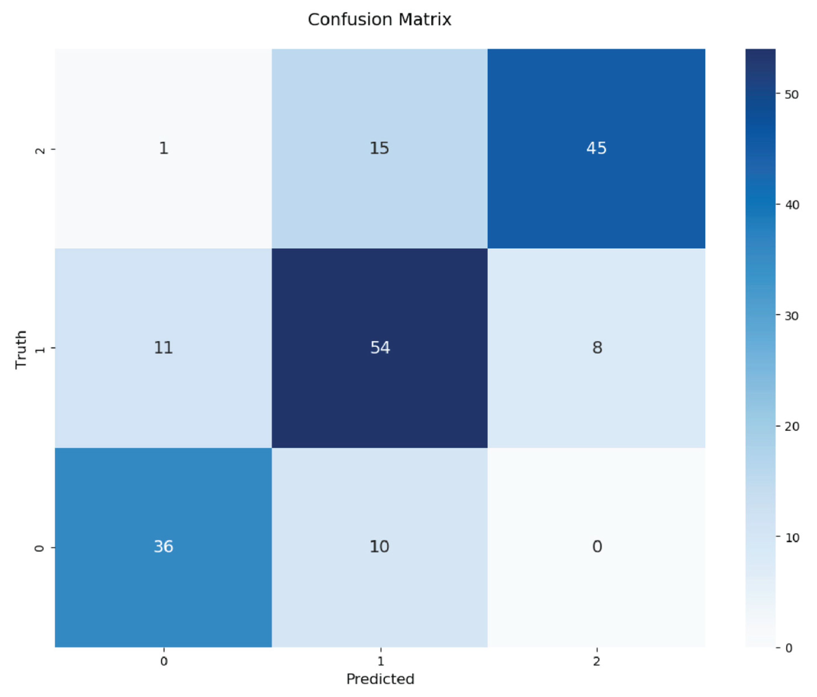

Table A1.
Shows all the 16 input features used as input for the baseline model, their description, their SHAP values, and their data source.
Table A1.
Shows all the 16 input features used as input for the baseline model, their description, their SHAP values, and their data source.
| Feature name. | Description |
Mean Absolute SHAP (class ‘2’) |
Correlation | Source |
| CommercialA | Total floor area of commercial land use (bank, bar, cafe, commercial, restaurant, retail, etc) |
0.276235 | + | GIS & OSM |
| EducationA | Total floor area of educational land use including (college, language_school, kindergarten, university, etc) |
0.047702 | - | GIS & OSM |
| HealthA | Total floor area of health related land use including (clinic, dentist, doctors, hospital, nursing_home, etc) |
0.021966 | - | GIS & OSM |
| InstitutionA | Total floor area of institutional land use including (civic, fire_station, government, police, townhall, etc) |
0.016998 | - | GIS & OSM |
| RecreationalA | Total floor area of recreational land use (arts_centre, barn, bbq, church, community_centre, etc) |
0.032891 | - | GIS & OSM |
| ResidentialA | Total floor area of residential type of land use (apartments, detached, dormitory, house, residential etc.) |
0.102843 | + | GIS & OSM |
| TransportationA | Total floor area of transportation land use (bus_station, ferry_terminal, train_station, etc) |
0.091451 | + | GIS & OSM |
| WorkA | Total floor area of work related land use (coworking_space, industrial, office, warehouse, etc) |
0.016481 | + | GIS & OSM |
| FloorArea | Total footprint * Number of Floors of all buildings within the study area. | 0.190040 | + | GIS & OSM |
| RoadCount | Total number of road segment within the road networks within the study area |
0.476555 | + | GIS & OSM |
| GreenArea | Total floor area of leisure type of land use (park, garden, pitch, playground, etc) |
0.148018 | + | GIS & OSM |
| LandUseDiversity | Total types of land use within the study area | 0.952107 | + | GIS & OSM |
| TotalLandUse | Total count of all land use types within the study area | 0.109048 | + | GIS & OSM |
| BasedDensity | Municipality Population / Total Land Area (ha) | 0.818544 | + | e-Stats |
| TaxPayerPer | Number of Taxpayer / Municipality Population | 0.141565 | + | e-Stats |
| TaxIncome | Tax revenue of the Municipality | 0.214959 | + | e-Stats |
References
- Cervero, R.; Kockelman, K. Travel Demand and the 3Ds: Density, Diversity, and Design. Transp. Res. Part Transp. Environ. 1997, 2, 199–219. [CrossRef]
- Dobson, J.E.; Bright, E.A.; Coleman, P.R.; Durfee, R.C.; Worley, B.A. LandScan: A Global Population Database for Estimating Populations at Risk. Photogramm. Eng. Remote Sens. 2000, 66, 849–858. [CrossRef]
- Zhao, X.; Xia, N.; Xu, Y.; Huang, X.; Li, M. Mapping Population Distribution Based on XGBoost Using Multisource Data. IEEE J. Sel. Top. Appl. Earth Obs. Remote Sens. 2021, 14, 11567–11580. [CrossRef]
- Wu, C.; Murray, A.T. A Cokriging Method for Estimating Population Density in Urban Areas. Comput. Environ. Urban Syst. 2005, 29, 558–579. [CrossRef]
- Tobler, W.; Deichmann, U.; Gottsegen, J.; Maloy, K. World Population in a Grid of Spherical Quadrilaterals. Int. J. Popul. Geogr. 1997, 3, 203–225. [CrossRef]
- Rojradtanasiri, P.; Tamura, J.; Kobayashi, M. Estimating Ambient Population Density Using Physical Features from GIS and Machine Learning: A Study Based on Japanese Neighborhood. J. Asian Archit. Build. Eng. 2024, 0, 1–16. [CrossRef]
- Spatial without Compromise · QGIS Available online: https://www.qgis.org/ (accessed on 3 July 2026).
- Team, Q.W. QuickOSM—Download OSM Data Thanks to the Overpass API. You Can Also Open Local OSM or PBF Files. A Special Parser, on Top of OGR, Is … Available online: https://plugins.qgis.org/plugins/QuickOSM/ (accessed on 17 September 2025).
- モバイル空間統計 人口マップ Available online: https://mobakumap.jp/ (accessed on 9 December 2025).
- Terada, M.; Nagata, T.; Kobayashi, M. Population Estimation Technology for Mobile Spatial Statistics. NTT DOCOMO Tech. J. 2013, 14.
- Bishop, C.M. Pattern Recognition and Machine Learning; Information science and statistics; Springer: New York, 2006; ISBN 978-0-387-31073-2.
- Chen, T.; Guestrin, C. XGBoost: A Scalable Tree Boosting System. In Proceedings of the Proceedings of the 22nd ACM SIGKDD International Conference on Knowledge Discovery and Data Mining; ACM: San Francisco California USA, August 13 2016; pp. 785–794.
- View Data | Municipality Data | System of Social and Demographic Statistics(SSDS) | Search by Areas Available online: https://www.e-stat.go.jp/en/regional-statistics/ssdsview/municipality (accessed on 27 June 2024).
- Available online: https://scikit-learn/stable/modules/generated/sklearn.metrics.f1_score.html (accessed on 27 June 2024).
- Lundberg, S.M.; Lee, S.-I. A Unified Approach to Interpreting Model Predictions. In Proceedings of the Advances in Neural Information Processing Systems; Curran Associates, Inc., 2017; Vol. 30.
- Goldstein, A.; Kapelner, A.; Bleich, J.; Pitkin, E. Peeking Inside the Black Box: Visualizing Statistical Learning with Plots of Individual Conditional Expectation 2014.
- What Is an AI Model? | IBM Available online: https://www.ibm.com/think/topics/ai-model (accessed on 3 July 2026).
- Introducing Llama 3.1: Our Most Capable Models to Date Available online: https://ai.meta.com/blog/meta-llama-3-1/ (accessed on 3 July 2026).
- AIME 2025 Benchmark Leaderboard Available online: https://artificialanalysis.ai/evaluations/aime-2025 (accessed on 2 July 2026).
- Center for AI Safety; Phan, L.; Gatti, A.; Li, N.; Khoja, A.; Kim, R.; Ren, R.; Hausenloy, J.; Zhang, O.; Mazeika, M.; et al. A Benchmark of Expert-Level Academic Questions to Assess AI Capabilities. Nature 2026, 649, 1139–1146. [CrossRef]
- Tschisgale, P.; Maus, H.; Kieser, F.; Kroehs, B.; Petersen, S.; Wulff, P. Evaluating GPT- and Reasoning-Based Large Language Models on Physics Olympiad Problems: Surpassing Human Performance and Implications for Educational Assessment 2025.
- Koubaa, A.; Qureshi, B.; Ammar, A.; Khan, Z.; Boulila, W.; Ghouti, L. Humans Are Still Better than ChatGPT: Case of the IEEEXtreme Competition. Heliyon 2023, 9. [CrossRef]
- II, M.B.; Katz, D.M. GPT Takes the Bar Exam 2022.
- Jammal, A.A.; Thompson, A.C.; Mariottoni, E.B.; Berchuck, S.I.; Urata, C.N.; Estrela, T.; Wakil, S.M.; Costa, V.P.; Medeiros, F.A. Human Versus Machine: Comparing a Deep Learning Algorithm to Human Gradings for Detecting Glaucoma on Fundus Photographs. Am. J. Ophthalmol. 2020, 211, 123–131. [CrossRef]
- Salinas, M.P.; Sepúlveda, J.; Hidalgo, L.; Peirano, D.; Morel, M.; Uribe, P.; Rotemberg, V.; Briones, J.; Mery, D.; Navarrete-Dechent, C. A Systematic Review and Meta-Analysis of Artificial Intelligence versus Clinicians for Skin Cancer Diagnosis. Npj Digit. Med. 2024, 7, 125. [CrossRef]
- Shehu, H.A.; Browne, W.; Eisenbarth, H. A Comparison of Humans and Machine Learning Classifiers Detecting Emotion from Faces of People with Different Coverings 2021.
- Cowley, H.P.; Natter, M.; Gray-Roncal, K.; Rhodes, R.E.; Johnson, E.C.; Drenkow, N.; Shead, T.M.; Chance, F.S.; Wester, B.; Gray-Roncal, W. A Framework for Rigorous Evaluation of Human Performance in Human and Machine Learning Comparison Studies. Sci. Rep. 2022, 12, 5444. [CrossRef]
- Rate Limits | OpenAI API Available online: https://developers.openai.com/api/docs/guides/rate-limits (accessed on 3 July 2026).
- Bergmann, D. What Is a Context Window? | IBM Available online: https://www.ibm.com/think/topics/context-window (accessed on 3 July 2026).
- Dong, Z.; Li, J.; Men, X.; Zhao, W.X.; Wang, B.; Tian, Z.; Chen, W.; Wen, J.-R. Exploring Context Window of Large Language Models via Decomposed Positional Vectors. Adv. Neural Inf. Process. Syst. 2024, 37, 10320–10347.
- Farquhar, S.; Kossen, J.; Kuhn, L.; Gal, Y. Detecting Hallucinations in Large Language Models Using Semantic Entropy. Nature 2024, 630, 625–630. [CrossRef]
- Sarmadi, H.; Wahab, I.; Hall, O.; Rögnvaldsson, T.; Ohlsson, M. Human Bias and CNNs’ Superior Insights in Satellite Based Poverty Mapping. Sci. Rep. 2024, 14, 22878. [CrossRef]
- What Are Convolutional Neural Networks? | IBM Available online: https://www.ibm.com/think/topics/convolutional-neural-networks (accessed on 3 July 2026).
- Ahn, D.; Yang, J.; Cha, M.; Yang, H.; Kim, J.; Park, S.; Han, S.; Lee, E.; Lee, S.; Park, S. A Human-Machine Collaborative Approach Measures Economic Development Using Satellite Imagery. Nat. Commun. 2023, 14, 6811. [CrossRef]
- Panczak, R.; Charles-Edwards, E.; Corcoran, J. Estimating Temporary Populations: A Systematic Review of the Empirical Literature. Humanit. Soc. Sci. Commun. 2020, 6, 1–10. [CrossRef]
- OpenAI | Research & Deployment Available online: https://openai.com/ (accessed on 2 July 2026).
- K. Suresh, V.; Rawat, S. GPT Takes the SAT: Tracing Changes in Test Difficulty and Students’ Math Performance; 2025;
- The SAT—SAT Suite | College Board Available online: https://satsuite.collegeboard.org/sat (accessed on 2 July 2026).
- Workspace, G. Google Forms: Online Form Builder Available online: https://workspace.google.com/products/forms/ (accessed on 3 July 2026).
- Confusion_matrix Available online: https://scikit-learn/stable/modules/generated/sklearn.metrics.confusion_matrix.html (accessed on 27 June 2024).
- Hello GPT-4o Available online: https://openai.com/index/hello-gpt-4o/ (accessed on 3 July 2026).
- GPT-5 Is Here Available online: https://openai.com/gpt-5/ (accessed on 3 July 2026).
- Gemini 2.5 Flash | Gemini API Available online: https://ai.google.dev/gemini-api/docs/models/gemini-2.5-flash (accessed on 3 July 2026).
- Claude Sonnet Available online: https://www.anthropic.com/claude/sonnet (accessed on 3 July 2026).
- Grok 3 Beta — The Age of Reasoning Agents Available online: https://x.ai/news/grok-3 (accessed on 3 July 2026).
- Krugman, P. A Dynamic Spatial Model; National Bureau of Economic Research: Cambridge, MA, 1992; p. w4219;
Figure 1.
Methodology Overview.
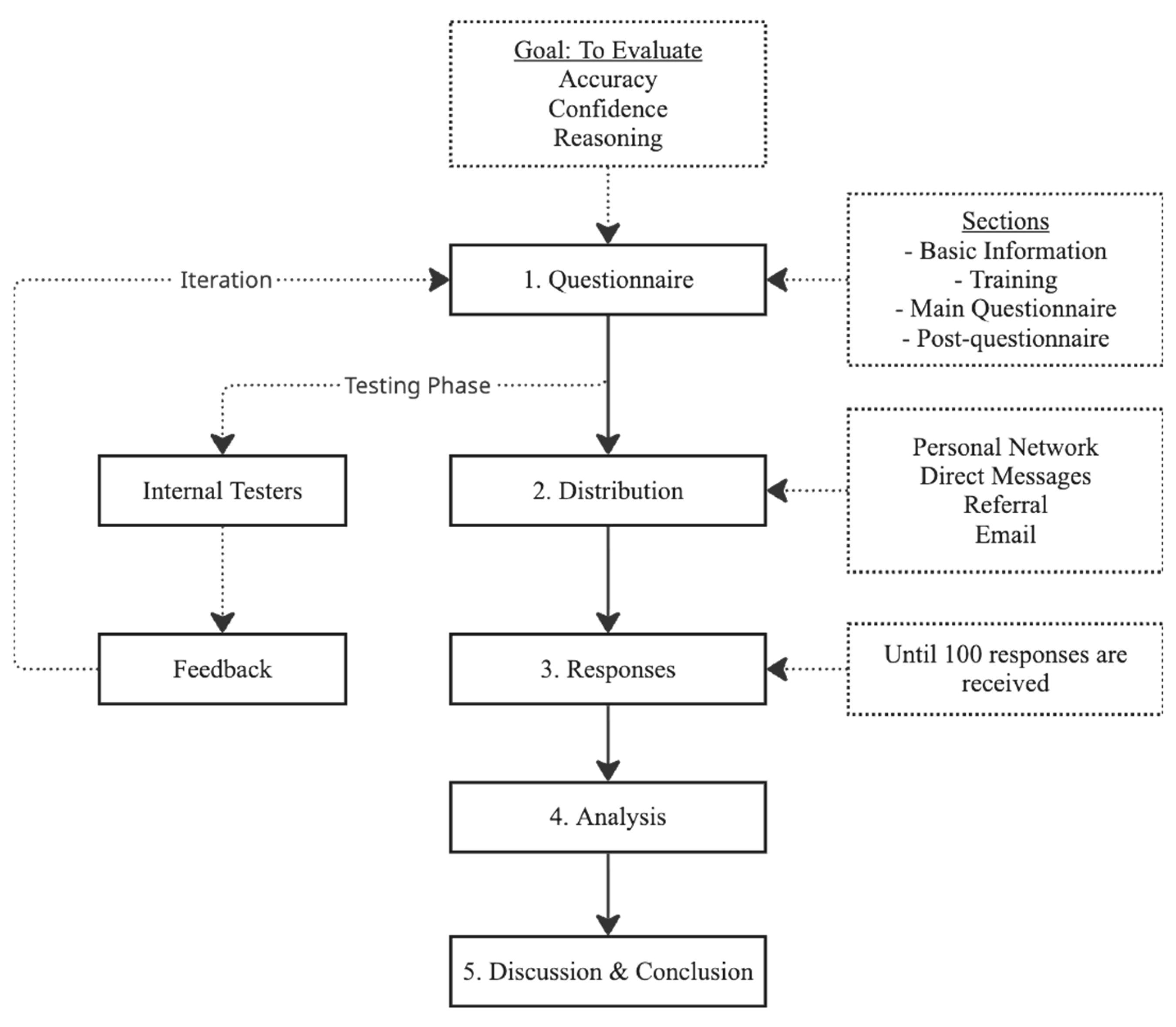
Figure 2.
Example of Q1 (Accuracy), Q2 (Reasoning), and Q3 (Confidence).
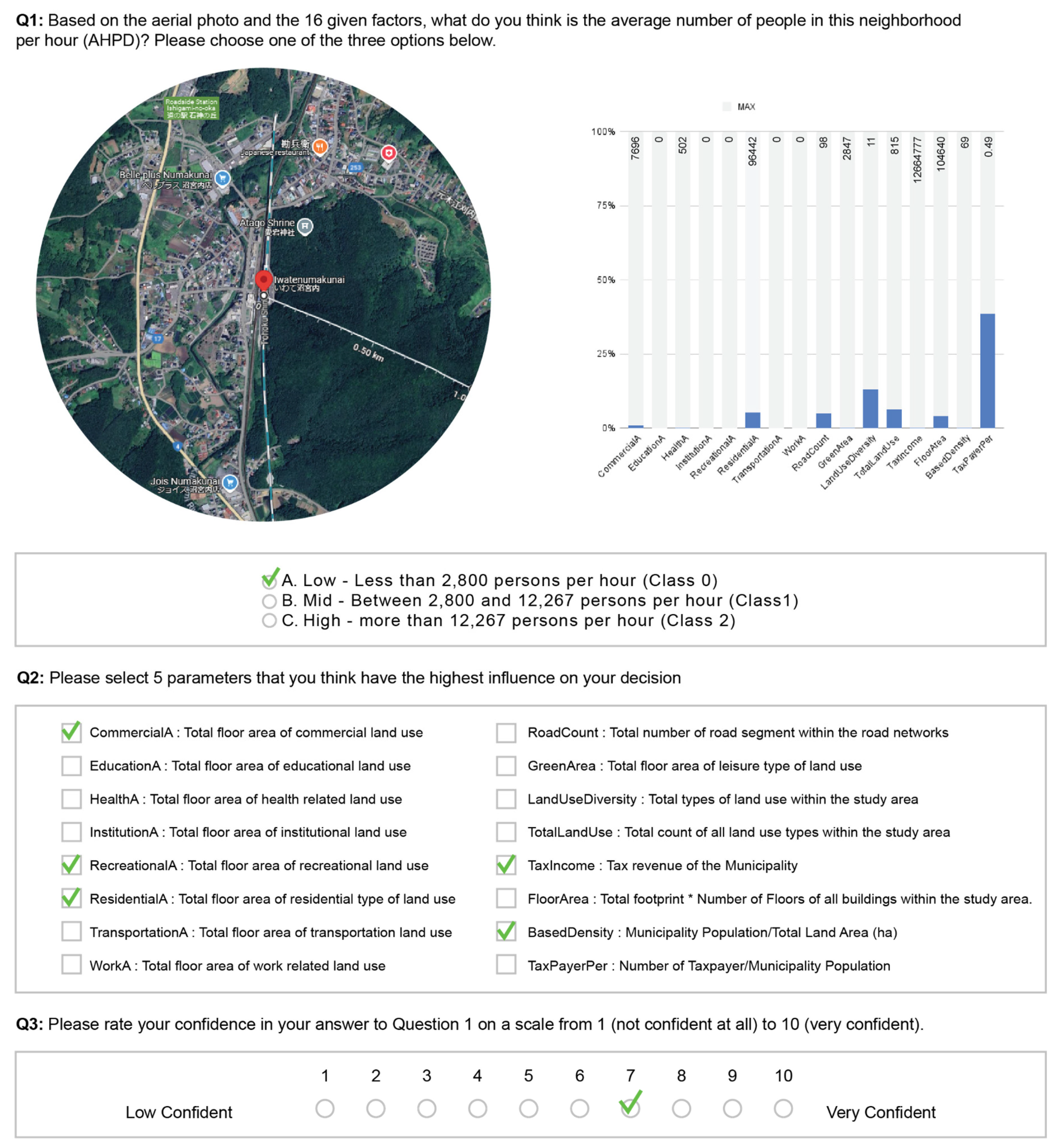
Figure 3.
Showing the score of all the respondents.
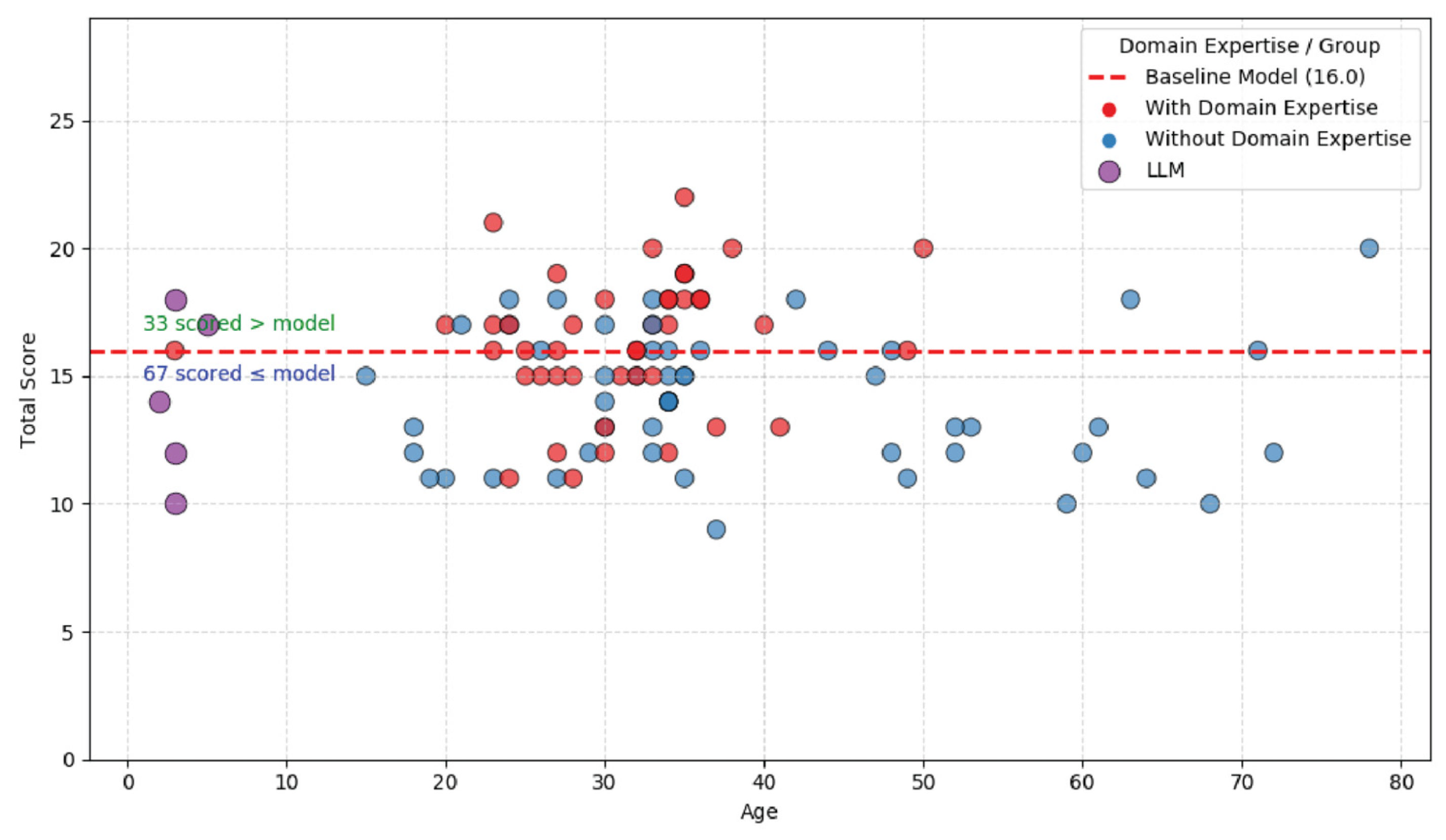
Figure 4.
Showing the score of all respondents along with the minimum and maximum score for each subgroup.
Figure 4.
Showing the score of all respondents along with the minimum and maximum score for each subgroup.
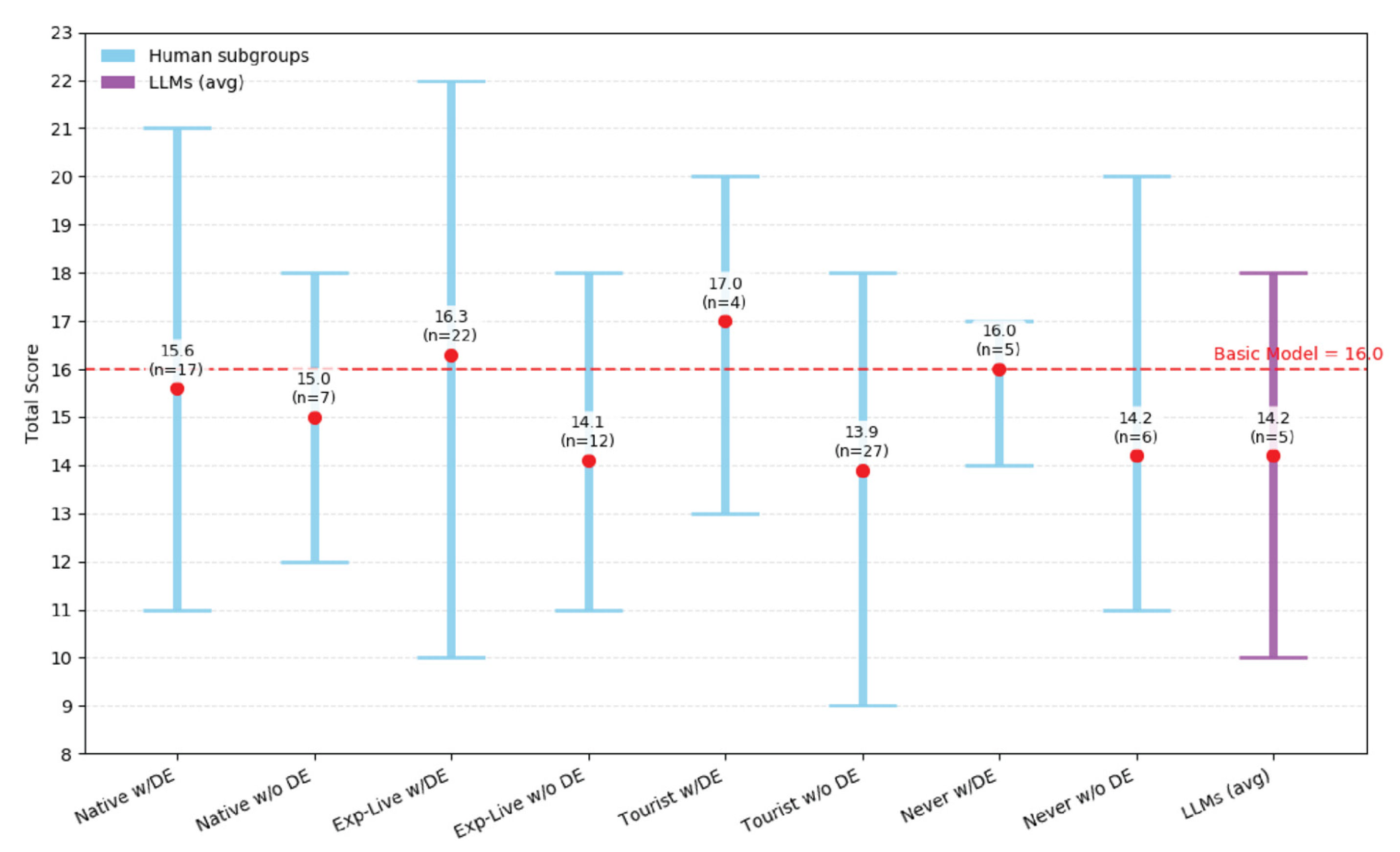
Figure 5.
Showing the reasoning score for humans (blue), AI models (purple), and the baseline model (grey).
Figure 5.
Showing the reasoning score for humans (blue), AI models (purple), and the baseline model (grey).
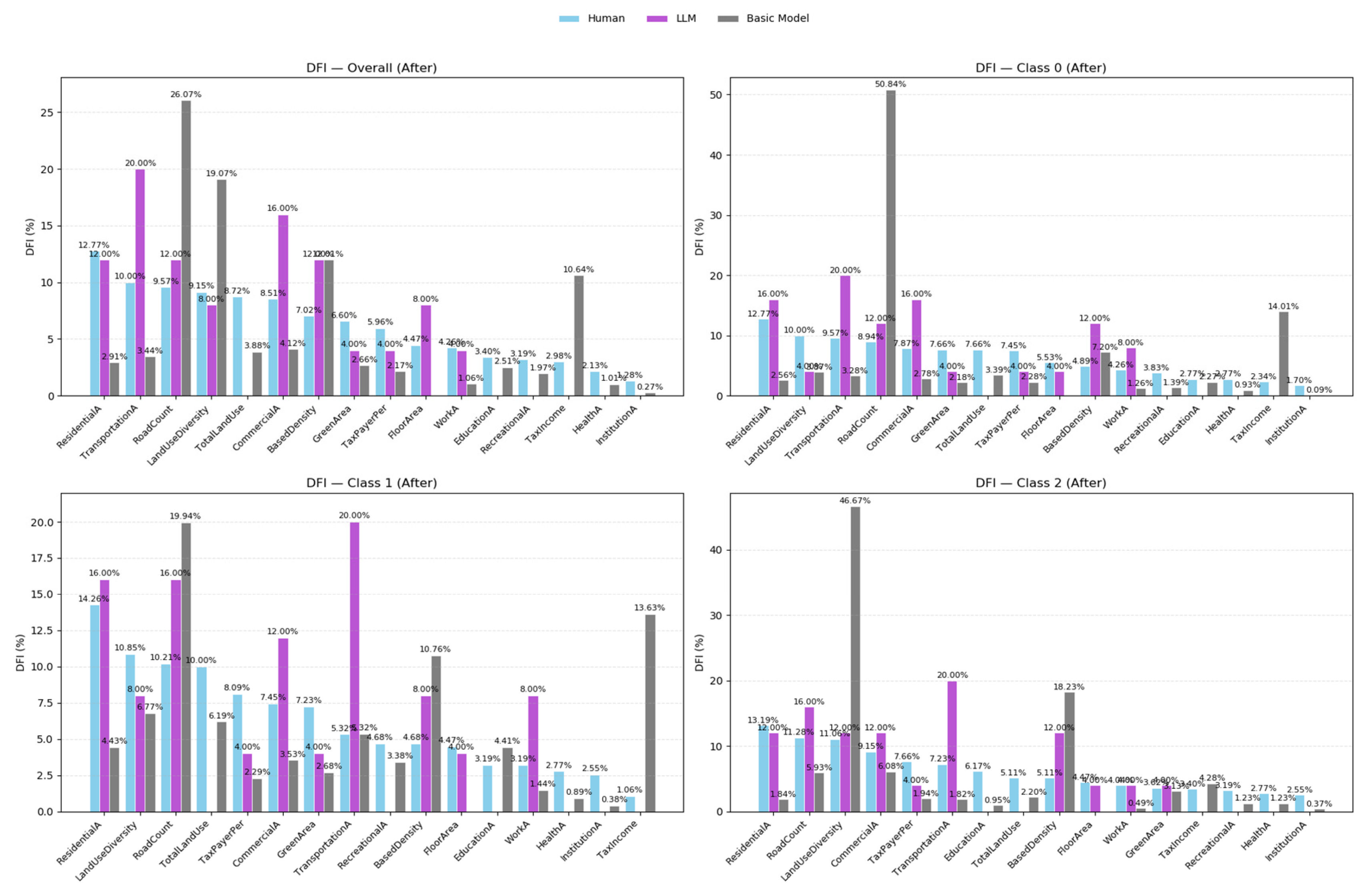
Figure 6.
Showing the correctness and confidence scores for each respondent types by question, with example images of selected images of selected questions.
Figure 6.
Showing the correctness and confidence scores for each respondent types by question, with example images of selected images of selected questions.
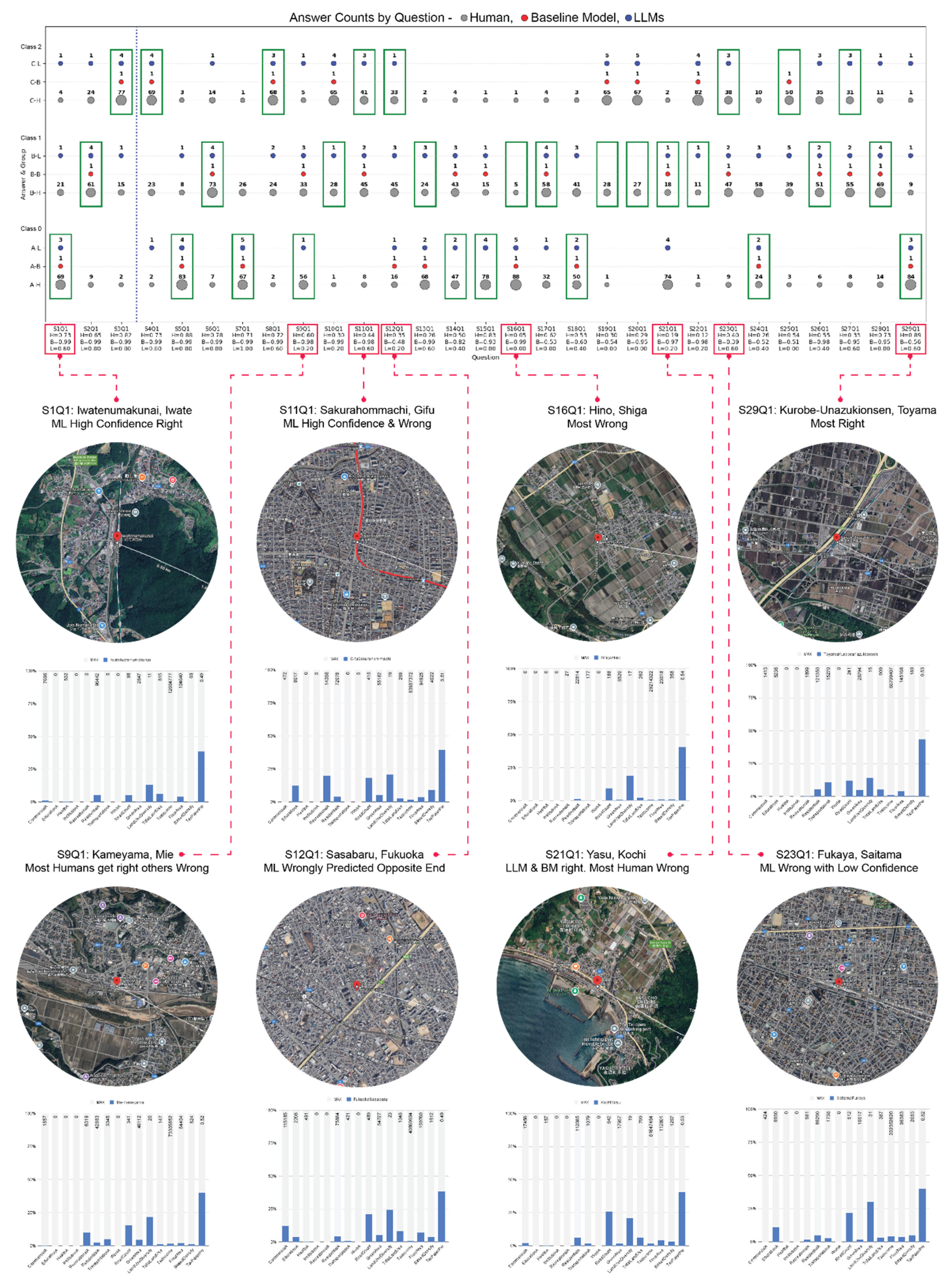
Table 1.
List of 29 neighborhoods used in the questionnaire (3 Training + 26 Main Questionnaire) along with the model’s confidence scores.
Table 1.
List of 29 neighborhoods used in the questionnaire (3 Training + 26 Main Questionnaire) along with the model’s confidence scores.
|
C0 P0 (Correct) |
C0 P1 (Over Est.) |
C0 P2 (Over Est.) |
C1 P1 (Correct) |
C1 P0 (Under Est.) |
C1 P2 (Over Est.) |
C2 P2 (Correct) |
C2 P1 (Under Est.) |
C2 P0 (Under Est.) |
|
Iwatenuma- kunai, Iwate (0.999) ET |
Kameyama, Mie/ (0.983) H |
- |
Kokubu, Kagoshima (0.997) ET |
Hino, Shiga (0.998) H |
Sakuramachi, Nagasaki (0.996) H |
Gojo, Kyoto (0.999) ET |
Fukaya, Saitama, (0.988) H |
Sasabaru, Fukuoka (0.488) H |
|
Daishaka, Aomori (0.998) E |
Yodoe, Tottori (0.936) H |
- |
Shimodate, Ibaraki (0.997) E |
Tsubata, Ishikawa (0.997) H |
Miebashi, Okinawa (0.989) H |
Fushimi, Aichi (0.999) E |
SakuraHom- machi, Gifu (0.983) H |
- |
|
Nahari, Kochi (0.997) E |
Kesennuma, Miyagi (0.821) H |
- |
Shirakawa, Fukushima (0.994) E |
Yasu, Kochi (0.997) H |
Kofu, Yamanashi (0.957) H |
Kamimaezu, Aichi (0.998) E |
Yokkaichi, Mie (0.953) H |
- |
| | 30 more | |
| 4 more | |
- | | 48 more | |
| 5 more | |
| 2 more | |
| 39 more | |
| 9 more | |
- |
|
Urasa, Niigata (0.601) M |
Chuden, Tokushima / (0.602) |
- |
Kiyotake, Miyazaki (0.532) M |
Sembokucho, Iwate (0.831) |
Tottori, Tottori (0.697) |
Kashiwa, Chiba (0.544) M |
Akita, Akita, (0.584) |
- |
|
Unazuki- Onsen, Toyama (0.566) M |
Obama, Fukui (0.555) |
- | Kyozuka, Okinawa (0.519) |
Nirasaki, Yamanashi (0.768) |
Minami Kofu, Yamanashi (0.604) |
Miyazaki, Miyazaki (0.536) |
Maebashi, Gumma, (0.561) |
- |
|
Yuasa, Wakayama (0.397) M |
Tamura, Fukushima / (0.516) |
- |
Inarimachi, Toyama (0.511) M |
Hizen Kashima, Saga (0.553) |
Saidaiji, Okayama (0.507) |
DaigakuByoin -mae, Nagasaki (0.525) M |
Awa-Tomida, Tokushima (0.522) |
- |
* E = Easy, M = Medium, H = Hard, ET = Easy questions used for training (underlined), Main Questionnaire = Bold, C = Correct Class, P = Predicted Class.
Table 2.
Showing the overall structure and which questionnaire item evaluates which metric.
| Metric | Basic Info Section | Training Section | Main Section | Post Section |
| Accuracy | - | S1Q1-S3Q1 (n=3) |
S4Q1-S29Q1 (n=26) |
- |
| Reasoning | Pre-Q6 (Opt., n=1) |
S1Q2-S3Q2 (Opt., n=3) |
S27Q2-S29Q2 (n=3) |
Post-Q4 (n=1) |
| Confidence | - | S1Q3-S3Q3 (n=3) |
S4Q3-S29Q3 (n=26) |
Post-Q1 (n=1) |
* S = Set, Q = Question, Opt. = Optional question, n = total number of item.
Table 3.
Showing the overall number (n) of respondents in each demographic group and their average score (s).
Table 3.
Showing the overall number (n) of respondents in each demographic group and their average score (s).
| Total Human Respondents (n=94, s=15.1) / min s= 9, max s=22 | ||
| Experience in Japan |
Without Domain Expertise (n = 49, s=14.5) |
With Domain Expertise (n=45, s=15.8) |
| Native Japanese (n=24, s=15.5) | n=9, s=15.2 | n=15, s=15.8 |
| Experienced Living in Japan (n=32, s=15.7) | n=13, s=15.3 | n=19, s=16.0 |
| Visited Japan as Tourist (n=29, s=14.1) | n=25, s=13.8 | n=4, s=16.2 |
| Never been to Japan Before (n=9, s=15.0) | n=2, s=15.5 | n=7, s=14.9 |
| Baseline model (s=16) / Average AI models (s=14.2) GPT-4o (s=18), GPT-5 (s=17), Grok 3 (s=10), Gemini 2.5 Flash (s=12), Claude Sonnet 4 (s=14) | ||
Table 4.
Shows the top 5 features with the highest difference for each context between human and the baseline ML model.
Table 4.
Shows the top 5 features with the highest difference for each context between human and the baseline ML model.
| #1 | #2 | #3 | #4 | #5 | |
| Overall | RoadCount Diff 16.49 H (9.57) ML (26.07) AIs (2.42) |
LandUseDiversity Diff 9.91 H (9.14) ML (19.05) AIs (8.00) |
ResidentialA Diff -9.85 H (12.76) ML (2.91) AIs (12.00) |
TaxIncome Diff 7.66 H (2.97) ML (10.64) AIs (0) |
TransportationA Diff -6.56 H (10.0) ML (3.44) AIs (20.00) |
| Class 0 | RoadCount Diff 41.90 H (8.93) ML (50.83) AIs (12.00) |
TaxIncome Diff 11.66 H (2.34) ML (14.01) AIs (0) |
ResidentialA Diff -10.20 H (12.76) ML (2.55) AIs (16.00) |
TransportationA Diff -6.29 H (9.57) ML (3.27) AIs (20.00) |
LandUseDiversity Diff -6.12 H (10.00) ML (3.87) AIs (4.00) |
| Class 1 | TaxIncome Diff 12.56 H (1.06) ML (13.62) AIs (0) |
ResidentialA Diff -9.82 H (14.25) ML (4.43) AIs (16.00) |
RoadCount Diff 9.75 H (10.21) ML (19.93) AIs (16.00) |
BasedDensity Diff 6.08 H (4.68) ML (10.76) AIs (8.00) |
TaxPayerPer Diff -5.79 H (8.08) ML (2.29) AIs (4.0) |
| Class 2 | LandUseDiversity Diff 35.60 H (11.06) ML (46.66) AIs (12.00) |
BasedDensity Diff 13.12 H (5.10) ML (18.22) AIs (12.00) |
ResidentialA Diff -11.35 H (13.19) ML (1.84) AIs (12.00) |
TaxPayerPer Diff -5.71 H (7.65) ML (1.94) AIs (4.00) |
RoadCount Diff -5.41 H (7.23) ML (1.82) AIs (20.00) |
Disclaimer/Publisher’s Note: The statements, opinions and data contained in all publications are solely those of the individual author(s) and contributor(s) and not of MDPI and/or the editor(s). MDPI and/or the editor(s) disclaim responsibility for any injury to people or property resulting from any ideas, methods, instructions or products referred to in the content. |
© 2026 by the authors. Licensee MDPI, Basel, Switzerland. This article is an open access article distributed under the terms and conditions of the Creative Commons Attribution (CC BY) license (http://creativecommons.org/licenses/by/4.0/).
Copyright: This open access article is published under a Creative Commons CC BY 4.0 license, which permit the free download, distribution, and reuse, provided that the author and preprint are cited in any reuse.


