

Submitted:
17 July 2026
Posted:
20 July 2026
You are already at the latest version
Abstract
Industrial diagnostic systems increasingly combine machine-learning classifiers, temporal models, uncertainty surrogates, and explanation methods. Their operational use requires a separate mechanism that determines whether the available evidence is valid, mutually consistent, sufficient for a recommendation, or should instead lead to abstention or human escalation. This paper introduces the Diagnostic Evidence Governance Agent (DEGA), a deterministic agent that separates evidence generation from workflow governance. DEGA operates on immutable evidence objects, follows an explicit finite-state workflow, applies a higher-priority SafetyGuard, and records a hash-linked audit trace supporting deterministic replay. The architecture is demonstrated in an offline case study using eight DUDU-BLDC acquisitions, 200 non-overlapping windows, 28 current- and speed-based features, three classifiers, and four spline representations. Across 16 dependent acquisition-disjoint assignment views, mean acquisition-level macro-F1 was 0.875 for Logistic Regression and 0.667 for both tree-based classifiers. The pipeline produced 768 complete EvidenceBundles with reproducible scientific hashes. Explanation rankings were assignment-sensitive, with a mean top-10 Jaccard similarity of 0.318. Twelve representative DEGA executions ended in three escalations and nine no-decision outcomes, with complete audit chains and deterministic replay. The study demonstrates auditable, fail-closed governance of AI-supported diagnostic evidence without delegating workflow control to an AI agent.
Keywords:
diagnostic evidence governance
; deterministic agent
; Industrial Internet of Things
; trustworthy diagnostics
; auditability
; abstention
; finite-state machine
; spline modelling
; BLDC motor
1. Introduction
The Industrial Internet of Things (IIoT) has expanded condition monitoring from isolated measurements to connected diagnostic pipelines that combine sensing, communication, edge or cloud computation, and maintenance decision support [1,2,3]. This development extends the established condition-based and e-maintenance literature, in which measured equipment condition is converted into diagnostic or prognostic information for maintenance planning [4,5]. In rotating machinery and electrical drives, signal-processing and machine-learning methods now extract diagnostic information from current, vibration, speed, and other operating channels [6,7,8,9]. Predictive-maintenance studies consequently focus on increasingly capable classifiers, ensembles, and deep models [10,11,12].
Model performance is necessary, but it does not by itself define an operational diagnostic decision process. A deployed system must also establish whether the data are admissible, which model and reference versions produced the available outputs, whether heterogeneous evidence sources agree, and whether the evidence is sufficient for an automated recommendation. When these conditions are not met, a diagnostic workflow should abstain or transfer the case to human review rather than force an action. The reject-option literature formalizes abstention, uncertainty-quantification methods characterize predictive uncertainty, explainable-AI methods expose aspects of model behaviour, and human-in-the-loop approaches define roles for expert intervention [13,14,15,16]. Data-provenance and machine-learning-assurance research further emphasize traceability across computational lifecycles [17,18,19].
These research strands address essential parts of trustworthy diagnostics, but they operate at different levels. A classifier score, a distribution-deviation measure, a spline descriptor, and a feature attribution have different assumptions and interpretation limits. A model-native probability may be uncalibrated; a deviation score may be only a relative surrogate; a spline derivative may describe geometric change in an ordered sequence without representing physical degradation time; and feature importance expresses model reliance rather than causal physical relevance [20,21,22]. Ethical and assurance principles call for transparency, accountability, and human oversight [18,23], but they do not specify how a concrete diagnostic workflow should admit, combine, route, veto, and audit heterogeneous evidence artifacts.
The resulting gap is architectural rather than algorithmic. The literature provides sophisticated evidence generators and several partial mechanisms for uncertainty, abstention, explanation, provenance, and human oversight, but it does not provide a single deterministic governance contract for a multi-stage industrial diagnostic workflow. In particular, a transparent mechanism is needed to keep evidence generation separate from final workflow authorization, preserve the provenance and interpretation boundary of each evidence item, make abstention and escalation explicit outcomes, permit higher-priority safety rules to override a routing policy, and reproduce the complete decision path after execution.
This paper addresses that gap through the Diagnostic Evidence Governance Agent (DEGA). A DEGA is a deterministic diagnostic agent that governs evidence produced by external analytical modules. It does not plan autonomously, learn online, generate unrestricted responses, or modify its own execution rules. Machine-learning and other AI methods may generate evidence consumed by DEGA, while the governance workflow remains explicit, reproducible, and independently inspectable. The proposed architecture separates four responsibilities: versioned evidence generation, immutable aggregation in an EvidenceBundle, deterministic routing under an external higher-priority SafetyGuard, and mandatory audit with deterministic replay.
The architecture is demonstrated through an offline computational case study based on the public DUDU-BLDC dataset [24]. The study uses eight real acquisitions, 200 non-overlapping windows, acquisition-disjoint evaluation, three classifier families, four spline representations, explanation artifacts, and representative DEGA executions. The case study is intentionally bounded: it evaluates the governance and reproducibility of the computational workflow rather than operational coverage, run-to-failure prognosis, calibrated failure probabilities, or industrial safety certification.
The contributions are:
- a formal definition of DEGA as a deterministic governance layer independent of the mechanisms that generate diagnostic evidence;
- an explicit 11-state workflow with distinct recommendation, escalation, no-decision, and mandatory audit states;
- a higher-priority SafetyGuard that can override policy-proposed transitions when evidence or integrity requirements are not met;
- a structured evidence representation that preserves traceability across data, models, configurations, reference profiles, and explanation outputs;
- hash-linked audit records and deterministic replay of evidence and DEGA executions; and
- a bounded DUDU-BLDC case study demonstrating the complete workflow and its interpretation limits.
2. Background and Design Requirements
2.1. Diagnostic Signals and Domain-Grounded Interpretation
In the condition monitoring of electrical machines, a comprehensive diagnostic approach typically incorporates multiple physical modalities. Common sources include mechanical vibrations (the industry standard for detecting bearing defects and rotor unbalance), operating temperature (a critical safety parameter), electromagnetic torque, and phase currents. However, in this study, the interpretative examples and feature extraction pipelines are strictly limited to phase current and rotational speed, as these are the primary synchronized measurement channels available in the utilized DUDU-BLDC dataset [6,7].
In this framework, the phase current serves as the primary channel for evaluating the electrical load, inverter operation dynamics, and the physical consequences of partial rotor demagnetization. Conversely, the rotational speed channel is essential for assessing mechanical stability, speed ripple, and the impact of physical anomalies on the motor’s kinematic behavior.
To translate raw time-series data into actionable knowledge, the current and speed signals are transformed into an intermediate layer of diagnostic features. For the proposed diagnostic workflow, the following classical indicators form the core of the analysis: root mean square (RMS), standard deviation, kurtosis, crest factor, and the spectral center. RMS represents the effective value of current or speed and provides a baseline indicator of global signal level and electrical or mechanical load. Standard deviation quantifies signal variability. Kurtosis and crest factor describe impulsiveness and sensitivity to rare high-energy deviations, whereas the spectral center summarizes shifts in the distribution of frequency-domain energy.
While the primary analysis relies on static window features, the advanced modelling framework also utilizes derivative trend features, such as spline slope. These trend indicators are constructed sequentially across ordered records, functioning as an additional mathematical layer rather than requiring a complete recalculation of the raw waveforms.
The implemented extractor computes 28 case-local features rather than using a globally precomputed feature table. Harmonic amplitudes at 1x, 2x, and 3x were considered because of their established diagnostic value in electrical machines [25,26], but they were not included in the final feature vector: a defensible case-local rotational fundamental could not be established for every canonical window. The study therefore uses broad spectral energy, centroid, and bandwidth descriptors and explicitly records the harmonic features as unavailable rather than replacing them with arbitrary frequency bins.
Providing a robust, physically grounded explanation for a model’s decision is a prerequisite for trustworthy diagnostic support. For the Healthy class, RMS and standard-deviation features of current and speed are expected to remain comparatively stable. In the presence of mechanical damage, the diagnostic signature is expected to be dominated by kinematic instability, whereas partial rotor demagnetization can alter the required electrical effort. The combined mechanical–electrical condition may introduce simultaneous deviations across both domains and is therefore a useful case for examining evidence conflict.
Table 1 retains the domain interpretation proposed for the principal evidence groups while explicitly separating admissible interpretation from unsupported causal claims.
2.2. Spline-Based Temporal Evidence
Early and reliable fault detection in Brushless DC (BLDC) motors is critical for improving system reliability and reducing unplanned downtime in modern industrial applications. Unexpected failures in electrical machines on production lines lead not only to process halts but also to increased maintenance costs, reduced energy efficiency, and compromised product quality. Standard condition monitoring approaches typically rely on the segmentation of vibration and current signals into short measurement windows, followed by the extraction of discrete time- and frequency-domain features.
However, in real-world operational environments, traditional indicators such as RMS and crest factor can exhibit high variance. They may fluctuate between consecutive measurement windows because of sensor noise, inverter interference, and non-linear load variations. Basing diagnostic decisions solely on a single noisy reading introduces a risk of false alarms or missed early-stage faults. It is therefore useful to supplement isolated-window interpretation with a continuous representation of changes across ordered windows.
This paper integrates spline functions as a mathematical smoothing and data-preparation layer for an advanced diagnostic reasoning module [27,28]. Spline models enable the extraction of derivative indicators from the fitted trend, complementing feature-based motor diagnostics and prognosis-oriented trend representations [29]. The first derivative represents the local rate of change, whereas the second derivative represents the local change in slope.
In the present dataset, these derivatives are defined with respect to normalized window order, not physical degradation time. The wording “rate of degradation”, “damage acceleration”, “failure onset”, and “remaining useful life” is therefore intentionally avoided.
Global polynomial regression is unsuitable for local trend description because high-order fits may introduce unwanted oscillations across the measurement domain [27]. Spline functions provide a flexible alternative through their piecewise-polynomial structure. Smoothing splines balance fit and smoothness; B-splines represent the curve through local basis functions; P-splines add a penalty for excessive coefficient variation; and monotonic splines impose shape constraints that may be useful only when monotonicity is physically justified.
Special emphasis is placed on penalized B-splines because the complexity penalty controls excessive local variation. This can reduce the effect of isolated spikes and requires an explicit choice of the penalty parameter. A reference profile can additionally be constructed from Healthy data, allowing the current fitted sequence to be compared with a documented baseline.
The reference used here is assignment-specific and training-only, rather than a global profile constructed from the entire dataset. The four implemented representations are not ranked as universally optimal; each produces a versioned temporal evidence object with fit diagnostics, derivatives, curvature, reference identity, and input-window hashes.
2.3. Explainability as Diagnostic Evidence
To ensure that a diagnostic workflow remains transparent, raw classification outputs should be paired with interpretable justifications. Global feature-attribution techniques, such as permutation importance, describe the macroscopic behaviour of a fitted model by measuring the decrease in predictive performance when a feature is shuffled.
For localized explanations, additive feature contributions can quantify how individual variables shift a model score. Methods such as LIME, SHAP, and partial-dependence profiles are relevant general-purpose tools for this task [15,22,30]; however, explanation methods must be distinguished from physical causal analysis.
Mathematical attributions may also be translated into rule-based statements for human operators. Explanation stability is an additional concern: if similar models or data partitions produce substantially different rankings, the explanation should be treated as assignment- or model-specific rather than universal.
The implemented study uses global permutation importance, an exact local Logistic Regression logit decomposition, and a descriptive cross-assignment stability analysis. It does not report SHAP or partial-dependence experiments. Explainability is consequently treated as another evidence source, never as independent authority to issue an action.
2.4. Requirements for Evidence Governance
The reviewed evidence sources motivate five requirements. First, every evidence item must preserve data, model, configuration, and reference provenance. Second, unavailable evidence must be explicit rather than fabricated. Third, evidence generation must remain separate from action authorization. Fourth, the workflow must support recommendation, escalation, and no-decision as distinct outcomes. Fifth, every execution must be auditable and reproducible. These requirements define the role of DEGA in Section 3 and Section 4.
3. Diagnostic Data and Evidence Representation
3.1. Data Units and Feature Representation
The DUDU-BLDC dataset provides synchronized phase-current and rotational-speed measurements under four conditions: Healthy, Mech_Damage, Elec_Damage, and Mech_Elec_Damage [24]. The case study uses eight raw acquisitions, two per class. Each acquisition is divided into 25 non-overlapping windows of s; at 50 kHz, each window contains 40000 samples. The resulting corpus contains windows. The acquisition, not the window, is the independent source unit. Window-level observations are nested within acquisitions and are reported descriptively. Figure 1 summarizes the data hierarchy and the acquisition-disjoint assignment rule.
A deterministic case-local extractor computes 14 features from each channel: mean, population standard deviation, population variance, RMS, maximum, minimum, absolute peak, peak-to-peak range, population skewness, population excess kurtosis, crest factor, mean-removed Hann-window spectral energy, power-weighted spectral centroid, and power-weighted spectral bandwidth. Thus, each window is represented by
where a identifies the acquisition and identifies the window. Equation (1) defines the common input space for the classifier, reference, and temporal-evidence modules. Operations that require population fitting—scaling, imputation, model fitting, distribution-deviation fitting, or Healthy-reference construction—are applied only after the acquisition assignment is defined.
3.2. Temporal Spline Evidence
For each acquisition, the 25 feature vectors retain their original order. The independent variable for temporal modelling is the normalized window position
The coordinate in Equation (2) is dimensionless and records order only. Four implementations share a common interface: rolling smoothing spline, rolling B-spline, rolling P-spline, and rolling Healthy-relative spline. For a fitted sequence , the evidence object records the fitted value, first and second derivatives, curvature, fitting error, roughness, effective degrees of freedom, uncertainty surrogate, fit status, configuration hash, and source-window hashes. Curvature is defined as
The maximum of Equation (3) denotes the strongest geometric change in the ordered sequence. It is not interpreted as physical fault onset.
3.3. Training-Only References and Deviation Evidence
Each acquisition assignment contains exactly one Healthy acquisition in the training partition. Its windows define the assignment-specific Healthy reference; the held-out Healthy acquisition is excluded. A separate training-distribution deviation scorer standardizes the 28-dimensional vectors using training-only statistics and fits a Ledoit–Wolf covariance estimator. For a standardized held-out vector , the squared Mahalanobis distance is
where and the precision matrix are derived exclusively from the active training partition. The bounded score derived from Equation (4) is an uncalibrated out-of-distribution (OOD) surrogate that quantifies departure from the active training distribution.
3.4. Immutable Evidence Hierarchy
The evidence layer contains five nested record types. Window- and acquisition-level outputs are stored as WindowEvidence and AcquisitionEvidence; temporal, risk, and safety outputs are stored as TrendEvidence, RiskEvidence, and SafetyEvidence. These records are combined into an immutable EvidenceBundle containing the assignment, acquisition, classifier, source-window identities, feature schema, temporal model, Healthy reference, distribution-deviation scorer, explanation artifact, risk components, and scientific hashes. Ground-truth labels and correctness indicators are excluded from agent-consumable evidence. Figure 2 shows the resulting provenance-preserving hierarchy.
4. DEGA Architecture and Deterministic Workflow
4.1. Agent Definition
The diagnostic agent operates as a state-transition control mechanism that processes sensor data, evaluates data quality, models ordered diagnostic trends, extracts diagnostic features, and classifies the technical condition of the monitored object. It is formalised as a finite-state machine. This formulation represents a control mechanism for diagnostic workflow transitions. Dynamic modelling of the physical motor and stability analysis remain separate engineering tasks.
Furthermore, the agent does not function as an autonomous control system capable of independently stopping the motor. Instead, it is a condition-driven workflow designed to issue actionable recommendations, escalate uncertain or high-risk cases to a human operator, and maintain a fully auditable decision log. It evaluates measurable indicators at each stage to select the next processing step, following a fixed graph of states governed by data quality, classifier confidence, trend–classifier agreement, explanation availability, and risk thresholds. Every path through the automaton terminates in a mandatory audit state, producing a complete audit trail.
Formally, a DEGA implementation is represented as
where is the semantic state set, is the immutable evidence space, contains deterministic processing functions, is the routing-policy family, is the higher-priority SafetyGuard rule set, and is the audit log. Equation (5) separates the evidence-processing functions from the policy and governance constraints.
Figure 3 presents this separation as a layered architecture: analytical modules produce evidence, whereas DEGA controls admissibility, routing, terminal disposition, and audit.
4.2. Semantic State Model
The canonical state set contains 11 states (Table 2). The explicit state-machine representation follows established finite-state modelling principles, while its semantics are specific to diagnostic evidence governance [31]. The state names are semantic contracts rather than implementation labels.
Each state performs a predefined processing step and produces outputs that serve as inputs to subsequent states. Data validation checks the required channels, feature ranges, completeness, and integrity. Trend modelling attaches the fitted spline and its derivative descriptors. Diagnostic inference consumes the classifier evidence, and explanation generation attaches the available feature-attribution evidence. The decision check evaluates confidence, model agreement, and compound risk. It routes the case to recommendation, escalation, or no decision. Every path unconditionally leads to the audit state, which records the structured decision trace and the justification for the final action.
4.3. Routing Policies and SafetyGuard
Four routing policies are evaluated: a static transition-matrix policy, a deterministic posterior approximation, a policy using persisted Bayesian MCMC evidence, and a hybrid policy. For current state and evidence summary , a policy maps the current context to a preference distribution over admissible successor states:
The quantities in Equation (6) are preferences over workflow states, not probabilities of physical motor degradation. All persisted inputs are frozen and the proposed next state is selected deterministically with fixed tie handling.
The agent’s workflow is supervised by operational constraints to ensure safe and deterministic behaviour. These constraints form a higher-level control layer that operates independently of the routing preference. A transition with high preference may therefore be blocked if it violates safety, data-integrity, or explainability requirements. The constraint layer prevents the agent from making decisions without sufficient evidence, bypassing validation procedures, or producing outputs that lack confidence estimation, traceability, and justification. It also ensures that uncertain or conflicting cases are escalated and that unreliable inputs cannot lead to automated recommendations.
If is the transition selected by the policy, the executed transition is
where G is the external SafetyGuard and is the structured evidence available at the current state. Equation (7) formalizes policy precedence: the SafetyGuard evaluates the proposal but has authority over the executed transition. These overrides establish configured fail-closed routing in this software study; they do not prove real-world safety-risk reduction.
4.4. Audit and Deterministic Replay
Every execution reaches S10. Audit events include the EvidenceBundle hash, policy and configuration hashes, ordered state path, transition proposals, SafetyGuard evaluations, overrides, reason codes, and final outcome. Events are chained through previous-event and current-event hashes. Deterministic replay uses the same stored evidence and policy configuration to reproduce and verify the workflow state sequence, SafetyGuard result, final outcome, and execution hash. This implementation operationalizes reproducibility recommendations by persisting the inputs and identities required to repeat the computational decision path [19]. Figure 5 summarizes the audit–replay contract.
5. Computational Case-Study Protocol
Acquisition-Disjoint Assignments
Because the dataset contains two source acquisitions per class, one acquisition from each class is assigned to training and the other to held-out evaluation. The complete Cartesian design contains class-complete assignment views. Each view contains four training and four held-out acquisitions, corresponding to 100 windows in each partition, with zero acquisition and window overlap. The views are exhaustive but dependent because they reuse the same eight acquisitions (Figure 1).
Classifier and Aggregation Protocol
Logistic Regression (LR), Random Forest (RF) [32], and Histogram Gradient Boosting (HGB) are evaluated under frozen hyperparameters. All preprocessing and fitting are restricted to the active training acquisitions. The protocol therefore contains model runs. Each persisted pipeline is reloaded and checked for exact equivalence before generating held-out evidence. The 25 window probability vectors for each held-out acquisition are aggregated by coordinate-wise mean, producing 192 acquisition-level predictions. Model outputs are explicitly labelled as model-native, uncalibrated probabilities.
Temporal, Reference, Risk, and Explanation Evidence
The four spline representations are fitted to the ordered windows of each held-out acquisition. Healthy references and training-distribution deviation scorers are fitted separately for every assignment using training data only. The risk object stores decomposed contributions for classifier uncertainty, temporal uncertainty, distribution deviation, Healthy-reference deviation, and conflict evidence. Its combined score is an experimental aggregate that supports workflow routing by combining the configured uncertainty, deviation, and conflict components.
Explainability is evaluated through three bounded analyses: global permutation importance for the preregistered A00 RF model; exact local additive contributions for one LR case; and top-10 feature-set stability across the 16 dependent assignment views.
Representative DEGA Executions
Three natural persisted evidence scenarios are executed under each of the four routing policies, giving 12 runs. The purpose is to exercise workflow semantics, policy differences, SafetyGuard precedence, audit completeness, and deterministic replay. The experiment is designed to exercise workflow semantics, policy differences, SafetyGuard precedence, audit completeness, and deterministic replay across representative scenarios.
Evaluation Boundaries
Primary classifier metrics are acquisition-level macro-F1 and balanced accuracy; window-level metrics remain descriptive. The study reports no confidence intervals based on treating windows or assignment views as independent. It does not support claims about run-to-failure degradation, RUL, calibrated failure probability, open-world OOD detection, universal classifier superiority, production readiness, industrial safety certification, or generalization beyond the eight source acquisitions.
6. Results
6.1. Classifier Evidence
All 48 persisted classifier pipelines passed exact reload-equivalence verification. Across the 16 dependent assignment views, mean acquisition-level macro-F1 was 0.875 for LR and 0.667 for both RF and HGB (Figure 6). These values summarize reuse of the same eight acquisitions and should not be interpreted as estimates from 16 independent experiments.
Mean-probability aggregation from 25 windows to one acquisition improved LR performance but reduced macro-F1 for the two tree-based classifiers (Figure 7). Aggregation is therefore part of the evidence-generation design rather than an automatically beneficial post-processing step.
6.2. Spline, Reference, and Risk Evidence
The evidence pipeline produced 256 immutable TrendEvidence artifacts covering four spline representations. The repository audit showed that these artifacts persist scalar descriptors but not the ordered feature sequence, spline evaluation grid, derivative arrays, curvature trajectory, Healthy reference curve, or uncertainty band. Figure 8 therefore reports the complete scalar evidence that exists rather than reconstructing a fitted trajectory.
Assignment-specific training-only Healthy references were successfully generated for all 16 assignments. Healthy-relative distance separated several electrical and combined-fault acquisitions more strongly than mechanical-damage acquisitions, emphasizing that this score is reference- and fault-dependent rather than universal. Figure 9 further shows that the persisted risk components differ substantially in numerical resolution.
6.3. Explanation Evidence
For the preregistered A00 RF model, the largest mean decreases in held-out balanced accuracy under permutation were obtained for speed_rms (0.0610), speed_mean (0.0570), and speed_variance (0.0277). Figure 10 shows all 28 implemented features and the 30 persisted permutation repeats. These values describe reliance of one fitted model under the selected scoring rule, not causal physical importance. The exact LR decomposition reconstructed the selected local logit with residual .
Across the 120 unique off-diagonal pairs, the mean top-10 Jaccard similarity was 0.318 and the median was 0.333, minimum 0.053, and maximum 0.818. Several speed-domain features recurred, but the full ranking was strongly assignment-sensitive (Figure 11).
6.4. Evidence Completeness and DEGA Execution
The completed evidence layer contains 4800 window records, 192 acquisition records, 768 risk records, 768 safety projections, and 768 complete immutable EvidenceBundle objects. Scientific replay reproduced identical bundle hashes for all 768 bundles.
All 12 representative DEGA runs completed with valid audit chains and deterministic replay. The final outcomes were three escalations, nine no-decision outcomes, and zero recommendations. The static policy traversed the full diagnostic workflow and was redirected to escalation by the SafetyGuard in each scenario. The remaining policies moved from validation to no decision under the frozen evidence and routing contract. Figure 12 and Figure 13 show the terminal dispositions and the two realized state sequences.
The integrity checks are summarized in Figure 14. All 48 classifier pipelines also passed exact reload-equivalence verification, as reported above.
7. Discussion
7.1. The Gap Addressed by DEGA
The results support the architectural claim that evidence governance is a separate engineering problem from diagnostic model construction. A classifier identifies the class favoured by a fitted model; a spline represents geometric change in an ordered sequence; a deviation scorer compares a vector with a training distribution; and an explanation describes model reliance. None of these outputs alone specifies whether an operational recommendation is admissible. DEGA makes that decision boundary explicit and deterministic.
This complements, rather than replaces, work on predictive maintenance, uncertainty, selective classification, explainability, and human-in-the-loop systems [11,13,14,15,16]. The distinctive element is the integration of heterogeneous evidence into an immutable contract governed by a semantic workflow, an external SafetyGuard, distinct abstention states, and mandatory replayable audit.
7.2. Fail-Closed Behaviour
The 12 executions yielded no recommendations. In a deployment benchmark this would indicate zero automated coverage, but the present experiment has a narrower purpose: it verifies that insufficient or policy-incompatible evidence is not converted into a positive action. The separation between escalation and no decision is useful. Escalation indicates that the evidence justifies human review because of ambiguity, conflict, or risk; no decision indicates that the automated workflow lacks an admissible basis to proceed.
The result should not be interpreted as evidence that the current thresholds or policies are operationally optimal. Three policies terminate immediately after validation, and the static policy is overridden by the SafetyGuard. A deployment study would require larger independent data, explicit costs for false recommendations and unnecessary escalation, and pre-specified policy-tuning criteria.
7.3. Interpretation of Classifier, Spline, and Explanation Evidence
LR obtained the highest descriptive acquisition-level macro-F1, but the eight source acquisitions do not support universal model ranking. The opposing effects of window aggregation across classifiers reinforce the need to preserve aggregation rules as evidence provenance.
Spline descriptors provide useful temporal structure, but their meaning follows the independent variable. Here, u is normalized window order, so derivatives and curvature cannot be relabelled as physical degradation rate, damage acceleration, or fault onset. This claim discipline is itself part of evidence governance.
The explanation analysis separates numerical fidelity from stability. The LR contribution identity is exact for one frozen model and case, while the RF top-feature ranking varies substantially across acquisition assignments. Therefore, explanation correctness for a single model does not imply robustness to plausible changes in the training acquisitions.
7.4. Auditability and Limitations
Exact model reload, bundle-hash reproduction, complete audit chains, and deterministic replay show that the implemented scientific path is reproducible under the frozen protocol. Auditability does not establish physical correctness or industrial safety: a reproducible workflow can reproduce a flawed model or a poorly selected threshold. Its value is that the assumptions, evidence identities, policy proposals, overrides, and outcomes remain inspectable.
The principal limitation is the small number of independent source acquisitions. The study does not establish generalization to other motors, loads, sensors, laboratories, or fault severities. The ordered windows are not run-to-failure records. Model-native probabilities remain uncalibrated. The distribution-deviation score quantifies departure from the active training distribution and has been evaluated within the present closed dataset. The combined risk score is an experimental aggregate used by the workflow-routing logic, and the agent experiment covers three representative evidence scenarios. Hardware integration, timing guarantees, cybersecurity, operator-interface validation, and compliance with functional-safety or AI-governance standards remain outside the scope.
Future work will evaluate the same governance contract on larger longitudinal and multi-asset datasets, formally verify state and SafetyGuard invariants, and investigate AI-assisted evidence generation while retaining a deterministic governance boundary.
8. Conclusions
This paper introduced the Diagnostic Evidence Governance Agent (DEGA), a deterministic agent that separates the generation of diagnostic evidence from the authorization and auditing of workflow outcomes. DEGA combines immutable evidence objects, an explicit 11-state workflow, interchangeable routing policies, an external higher-priority SafetyGuard, distinct recommendation, escalation, and no-decision states, and mandatory deterministic replay.
The DUDU-BLDC case study demonstrated the complete computational path on real acquisitions. The pipeline produced acquisition-disjoint classifier evidence, spline descriptors over ordered windows, training-only references, explanation artifacts, risk evidence, and 768 reproducible EvidenceBundles. Twelve representative DEGA runs produced only escalation or no-decision outcomes, illustrating fail-closed execution under the frozen protocol rather than operational recommendation coverage.
Within the stated limits, the study shows that AI-supported diagnostics need not delegate workflow control to an AI agent. Analytical intelligence can remain modular, while the governance of evidence is deterministic, traceable, and reproducible.
Author Contributions
Conceptualization, W.B. (DEGA implementation concept and computational study design) and J.B. (diagnostic-evidence governance concept and overall research framing); methodology, W.B. (computational pipeline, evidence contracts, audit and replay protocol), J.B. (governance architecture and methodological boundaries), and K.J. (spline-based evidence representation); software, W.B. (ArticleV1 pipeline and DEGA implementation); validation, W.B. (software, evidence, audit and replay validation), K.J. (spline-method and descriptor validation), A.P. (domain interpretation of current- and speed-based diagnostic features), M.Z. (finite-state workflow, abstention and escalation logic), and J.B. (overall methodological validation); formal analysis, W.B. and J.B.; investigation, W.B., K.J., A.P. and M.Z.; resources, K.J. (DUDU-BLDC data resources) and J.B.; data curation, W.B. and K.J.; writing—original draft preparation, W.B. (implementation, protocol and results), K.J. (spline-based diagnostic evidence and trend representation), A.P. (BLDC diagnostic-signal interpretation and explainability background), M.Z. (deterministic workflow, finite-state logic, abstention, escalation and audit mechanisms), and J.B. (conceptual framing, literature synthesis, discussion and manuscript integration); writing—review and editing, W.B. and J.B.; visualization, W.B. and J.B.; supervision, J.B.; project administration, J.B. All authors have read and agreed to the published version of the manuscript.
Funding
This research received no external funding.
Institutional Review Board Statement
Not applicable.
Informed Consent Statement
Not applicable.
Data Availability Statement
The DUDU-BLDC dataset is publicly available at Zenodo (DOI: 10.5281/zenodo.15522163). Reprofducibility of the study is possible with software provided in a public repository (DOI: 10.5281/zenodo.21374984).
Acknowledgments
The authors acknowledge the contributors who supported the preparation and curation of the DUDU-BLDC dataset. During preparation of this manuscript, the authors used ChatGPT (OpenAI) for language editing, structural drafting, and assistance with LaTeX and figure-integration workflows. All generated material was reviewed, verified, and edited by the authors, who take full responsibility for the content of the publication.
Conflicts of Interest
The authors declare no conflicts of interest.
Abbreviations
The following abbreviations are used in this manuscript:
| BLDC | Brushless direct-current motor |
| DEGA | Diagnostic Evidence Governance Agent |
| FSM | Finite-state machine |
| HGB | Histogram Gradient Boosting |
| IIoT | Industrial Internet of Things |
| LR | Logistic Regression |
| ML | Machine learning |
| OOD | Out-of-distribution |
| P-spline | Penalized B-spline |
| RF | Random Forest |
| RMS | Root mean square |
| XAI | Explainable artificial intelligence |
References
- Xu, L.D.; He, W.; Li, S. Internet of Things in Industries: A Survey. IEEE Trans. Ind. Inform. 2014, 10, 2233–2243. [Google Scholar] [CrossRef]
- Boyes, H.; Hallaq, B.; Cunningham, J.; Watson, T. The Industrial Internet of Things (IIoT): An Analysis Framework. Comput. Ind. 2018, 101, 1–12. [Google Scholar] [CrossRef]
- Sisinni, E.; Saifullah, A.; Han, S.; Jennehag, U.; Gidlund, M. Industrial Internet of Things: Challenges, Opportunities, and Directions. IEEE Trans. Ind. Inform. 2018, 14, 4724–4734. [Google Scholar] [CrossRef]
- Jardine, A.K.S.; Lin, D.; Banjevic, D. A Review on Machinery Diagnostics and Prognostics Implementing Condition-Based Maintenance. Mech. Syst. Signal Process. 2006, 20, 1483–1510. [Google Scholar] [CrossRef]
- Muller, A.; Marquez, A.C.; Iung, B. On the Concept of E-Maintenance: Review and Current Research. Reliab. Eng. Syst. Saf. 2008, 93, 1165–1187. [Google Scholar] [CrossRef]
- Nandi, S.; Toliyat, H.A.; Li, X. Condition Monitoring and Fault Diagnosis of Electrical Motors—A Review. IEEE Trans. Energy Convers. 2005, 20, 719–729. [Google Scholar] [CrossRef]
- Henao, H.; Capolino, G.A.; Fernandez-Cabanas, M.; Filippetti, F.; Bruzzese, C.; Strangas, E.; Pusca, R.; Estima, J.; Riera-Guasp, M.; Hedayati-Kia, S.H. Trends in Fault Diagnosis for Electrical Machines: A Review of Diagnostic Techniques. IEEE Ind. Electron. Mag. 2014, 8, 31–42. [Google Scholar] [CrossRef]
- Liu, R.; Yang, B.; Zio, E.; Chen, X. Artificial Intelligence for Fault Diagnosis of Rotating Machinery: A Review. Mech. Syst. Signal Process. 2018, 108, 33–47. [Google Scholar] [CrossRef]
- Lei, Y.; Yang, B.; Jiang, X.; Jia, F.; Li, N.; Nandi, A.K. Applications of Machine Learning to Machine Fault Diagnosis: A Review and Roadmap. Mech. Syst. Signal Process. 2020, 138, 106587. [Google Scholar] [CrossRef]
- Susto, G.A.; Schirru, A.; Pampuri, S.; McLoone, S.; Beghi, A. Machine Learning for Predictive Maintenance: A Multiple Classifier Approach. IEEE Trans. Ind. Inform. 2015, 11, 812–820. [Google Scholar] [CrossRef]
- Carvalho, T.P.; Soares, F.A.A.M.N.; Vita, R.; Francisco, R.d.P.; Basto, J.P.; Alcala, S.G.S. A Systematic Literature Review of Machine Learning Methods Applied to Predictive Maintenance. Comput. Ind. Eng. 2019, 137, 106024. [Google Scholar] [CrossRef]
- Serradilla, O.; Zugasti, E.; Zurutuza, U. Deep Learning Models for Predictive Maintenance: A Survey, Comparison, Challenges and Prospects. Comput. Ind. 2020, 123, 103257. [Google Scholar] [CrossRef]
- Hendrickx, K.; Perini, L.; Van der Plas, D.; Meert, W.; Davis, J. Machine Learning with a Reject Option: A Survey. Inf. Fusion 2021, 69, 69–82. [Google Scholar] [CrossRef] [PubMed]
- Abdar, M.; Pourpanah, F.; Hussain, S.; Rezazadegan, D.; Liu, L.; Ghavamzadeh, M.; Fieguth, P.; Cao, X.; Khosravi, A.; Acharya, U.R.; et al. A Review of Uncertainty Quantification in Deep Learning: Techniques, Applications and Challenges. Inf. Fusion 2021, 76, 243–297. [Google Scholar] [CrossRef]
- Barredo Arrieta, A.; Diaz-Rodriguez, N.; Del Ser, J.; Bennetot, A.; Tabik, S.; Barbado, A.; Garcia, S.; Gil-Lopez, S.; Molina, D.; Benjamins, R.; et al. Explainable Artificial Intelligence (XAI): Concepts, Taxonomies, Opportunities and Challenges toward Responsible AI. Inf. Fusion 2020, 58, 82–115. [Google Scholar] [CrossRef]
- Mosqueira-Rey, E.; Hernandez-Pereira, E.; Alonso-Rios, D.; Bobes-Bascaran, J.; Fernandez-Leal, A. Human-in-the-Loop Machine Learning: A State of the Art. Artif. Intell. Rev. 2023, 56, 3005–3054. [Google Scholar] [CrossRef]
- Simmhan, Y.L.; Plale, B.; Gannon, D. A Survey of Data Provenance in E-Science. SIGMOD Rec. 2005, 34, 31–36. [Google Scholar] [CrossRef]
- Ashmore, R.; Calinescu, R.; Paterson, C. Assuring the Machine Learning Lifecycle: Desiderata, Methods, and Challenges. ACM Comput. Surv. 2021, 54, 1–39. [Google Scholar] [CrossRef]
- Sandve, G.K.; Nekrutenko, A.; Taylor, J.; Hovig, E. Ten Simple Rules for Reproducible Computational Research. PLoS Comput. Biol. 2013, 9, e1003285. [Google Scholar] [CrossRef] [PubMed]
- Altmann, A.; Tolosi, L.; Sander, O.; Lengauer, T. Permutation Importance: A Corrected Feature Importance Measure. Bioinformatics 2010, 26, 1340–1347. [Google Scholar] [CrossRef] [PubMed]
- Fisher, A.; Rudin, C.; Dominici, F. All Models Are Wrong, but Many Are Useful: Learning a Variable’s Importance by Studying an Entire Class of Prediction Models Simultaneously. J. Am. Stat. Assoc. 2019, 114, 1321–1338. [Google Scholar] [CrossRef]
- Lundberg, S.M.; Erion, G.; Chen, H.; DeGrave, A.; Prutkin, J.M.; Nair, B.; Katz, R.; Himmelfarb, J.; Bansal, N.; Lee, S.I. From Local Explanations to Global Understanding with Explainable AI for Trees. Nat. Mach. Intell. 2020, 2, 56–67. [Google Scholar] [CrossRef] [PubMed]
- Jobin, A.; Ienca, M.; Vayena, E. The Global Landscape of AI Ethics Guidelines. Nat. Mach. Intell. 2019, 1, 389–399. [Google Scholar] [CrossRef]
- Baranowski, J.; Bauer, W.; Jarzyna, K.; Paweł, P. DUDU-BLDC: Data set for diagnostic of Brushless DC motors with degrading magnets. 2025. [Google Scholar] [CrossRef]
- Thomson, W.T.; Fenger, M. Current Signature Analysis to Detect Induction Motor Faults. IEEE Ind. Appl. Mag. 2001, 7, 26–34. [Google Scholar] [CrossRef]
- Riba Ruiz, J.R.; Rosero, J.A.; Garcia Espinosa, A.; Romeral, L. Detection of Demagnetization Faults in Permanent-Magnet Synchronous Motors under Nonstationary Conditions. IEEE Trans. Magn. 2009, 45, 2961–2969. [Google Scholar] [CrossRef]
- Eilers, P.H.C.; Marx, B.D. Flexible Smoothing with B-Splines and Penalties. Stat. Sci. 1996, 11, 89–121. [Google Scholar] [CrossRef]
- Bartoszewski, B.; Jarzyna, K.; Baranowski, J. Diagnosis of Mechanical Rotor Faults in Drones Using Functional Gaussian Mixture Classifier. Aerospace 2024, 11, 743. [Google Scholar] [CrossRef]
- Shifat, T.A.; Yasmin, R.; Hur, J.W. A Data-Driven RUL Estimation Framework of Electric Motor Using Deep Electrical Feature Learning from Current Harmonics and Apparent Power. Energies 2021, 14, 3156. [Google Scholar] [CrossRef]
- Ribeiro, M.T.; Singh, S.; Guestrin, C. Why Should I Trust You? Explaining the Predictions of Any Classifier. In Proceedings of the 22nd ACM SIGKDD International Conference on Knowledge Discovery and Data Mining, 2016; pp. 1135–1144. [Google Scholar] [CrossRef]
- Lee, D.; Yannakakis, M. Principles and Methods of Testing Finite State Machines—A Survey. Proc. IEEE 1996, 84, 1090–1123. [Google Scholar] [CrossRef]
- Breiman, L. Random Forests. Mach. Learn. 2001, 45, 5–32. [Google Scholar] [CrossRef]
Figure 1.
Acquisition-disjoint organization of the DUDU-BLDC case study. Each of the four diagnostic classes contains two source acquisitions, and each acquisition contains 25 non-overlapping windows. For every assignment, one acquisition per class is used for training and the other for held-out evaluation. All class-complete choices are evaluated; because the same eight acquisitions are reused, these views are dependent rather than independent replications.
Figure 1.
Acquisition-disjoint organization of the DUDU-BLDC case study. Each of the four diagnostic classes contains two source acquisitions, and each acquisition contains 25 non-overlapping windows. For every assignment, one acquisition per class is used for training and the other for held-out evaluation. All class-complete choices are evaluated; because the same eight acquisitions are reused, these views are dependent rather than independent replications.
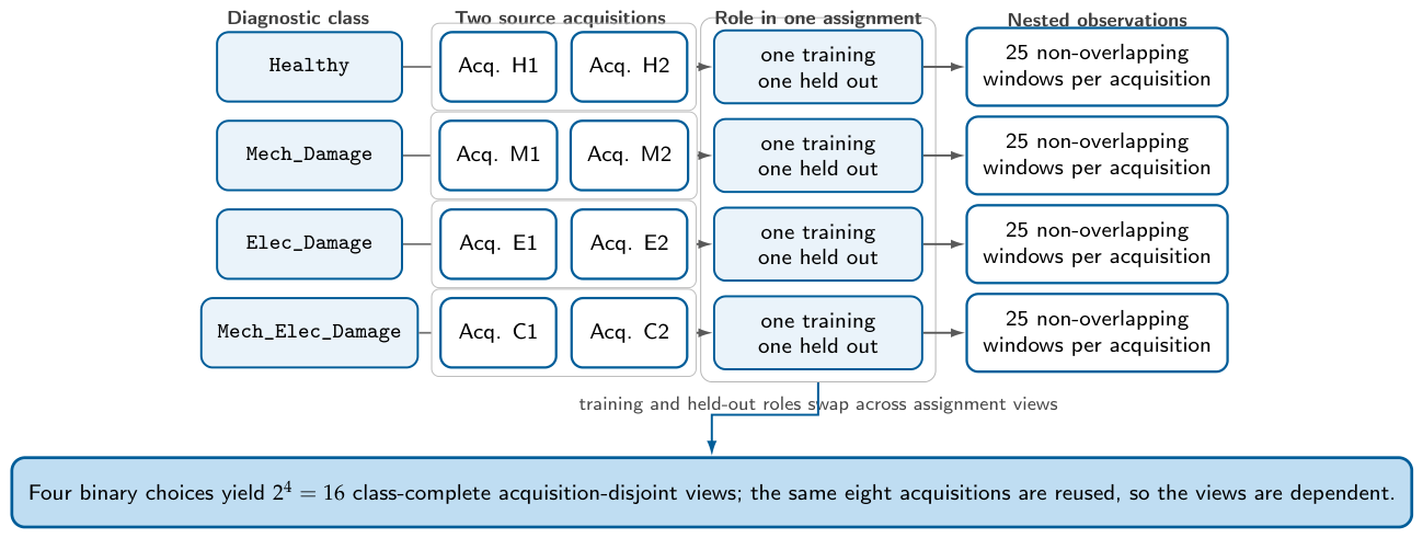
Figure 2.
Evidence hierarchy used by DEGA. Raw current and speed acquisitions are divided into windows and converted into classifier, acquisition-level, temporal, deviation, explanation, risk, and safety evidence. Each stage records the identities and hashes of its inputs. The final immutable EvidenceBundle contains no held-out ground-truth label, ensuring that evaluation information cannot influence the agent workflow.
Figure 2.
Evidence hierarchy used by DEGA. Raw current and speed acquisitions are divided into windows and converted into classifier, acquisition-level, temporal, deviation, explanation, risk, and safety evidence. Each stage records the identities and hashes of its inputs. The final immutable EvidenceBundle contains no held-out ground-truth label, ensuring that evaluation information cannot influence the agent workflow.
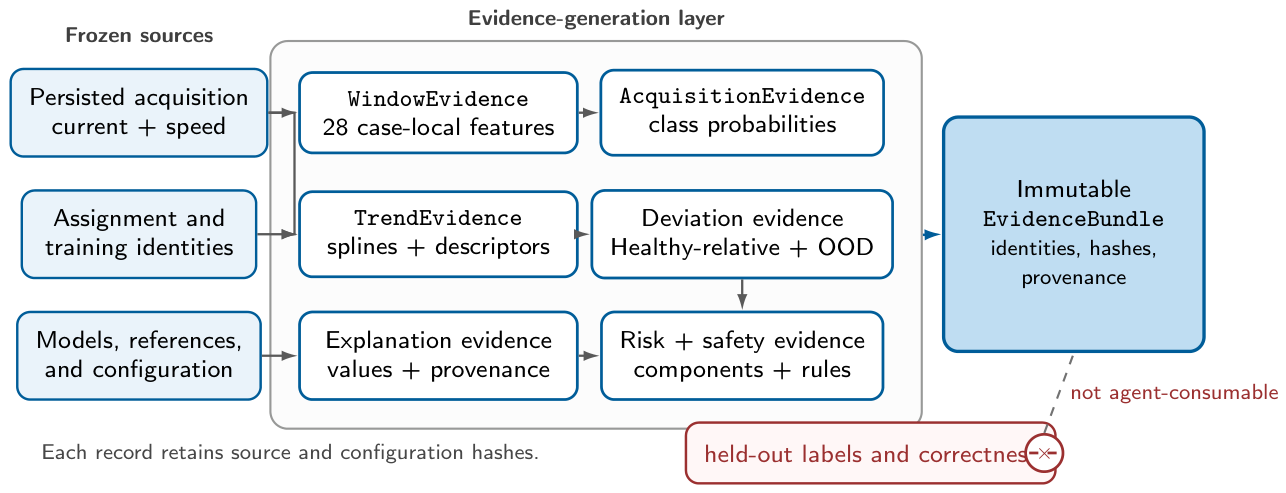
Figure 3.
Reference DEGA architecture. External analytical modules generate classifier, spline, explanation, distribution-deviation, risk, and safety evidence, which are collected in an immutable EvidenceBundle. Inside the deterministic governance boundary, the routing policy proposes a successor state, the higher-priority SafetyGuard validates or overrides that proposal using the same evidence context, and the DEGA finite-state workflow executes the final admissible transition. Recommendation, escalation, and no-decision are distinct terminal dispositions; each is followed by the same mandatory audit and deterministic-replay stage.
Figure 3.
Reference DEGA architecture. External analytical modules generate classifier, spline, explanation, distribution-deviation, risk, and safety evidence, which are collected in an immutable EvidenceBundle. Inside the deterministic governance boundary, the routing policy proposes a successor state, the higher-priority SafetyGuard validates or overrides that proposal using the same evidence context, and the DEGA finite-state workflow executes the final admissible transition. Recommendation, escalation, and no-decision are distinct terminal dispositions; each is followed by the same mandatory audit and deterministic-replay stage.
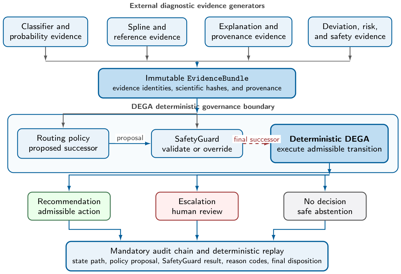
Figure 4.
Canonical 11-state DEGA finite-state machine. Solid blue arrows show the nominal path from acquisition (S0) through decision check (S6), followed by recommendation (S7), escalation (S8), or no decision (S9), and finally the mandatory audit state (S10). Failed validation may return S1 to S0. Dashed red routes enumerate the states from which escalation is admissible (S3–S6), while grey dash–dot routes enumerate no-decision transitions (S1–S3 and S5–S6). The diagram reproduces the canonical machine-readable edge set; the detailed predicates that activate each non-nominal edge remain in the state and SafetyGuard contracts.
Figure 4.
Canonical 11-state DEGA finite-state machine. Solid blue arrows show the nominal path from acquisition (S0) through decision check (S6), followed by recommendation (S7), escalation (S8), or no decision (S9), and finally the mandatory audit state (S10). Failed validation may return S1 to S0. Dashed red routes enumerate the states from which escalation is admissible (S3–S6), while grey dash–dot routes enumerate no-decision transitions (S1–S3 and S5–S6). The diagram reproduces the canonical machine-readable edge set; the detailed predicates that activate each non-nominal edge remain in the state and SafetyGuard contracts.
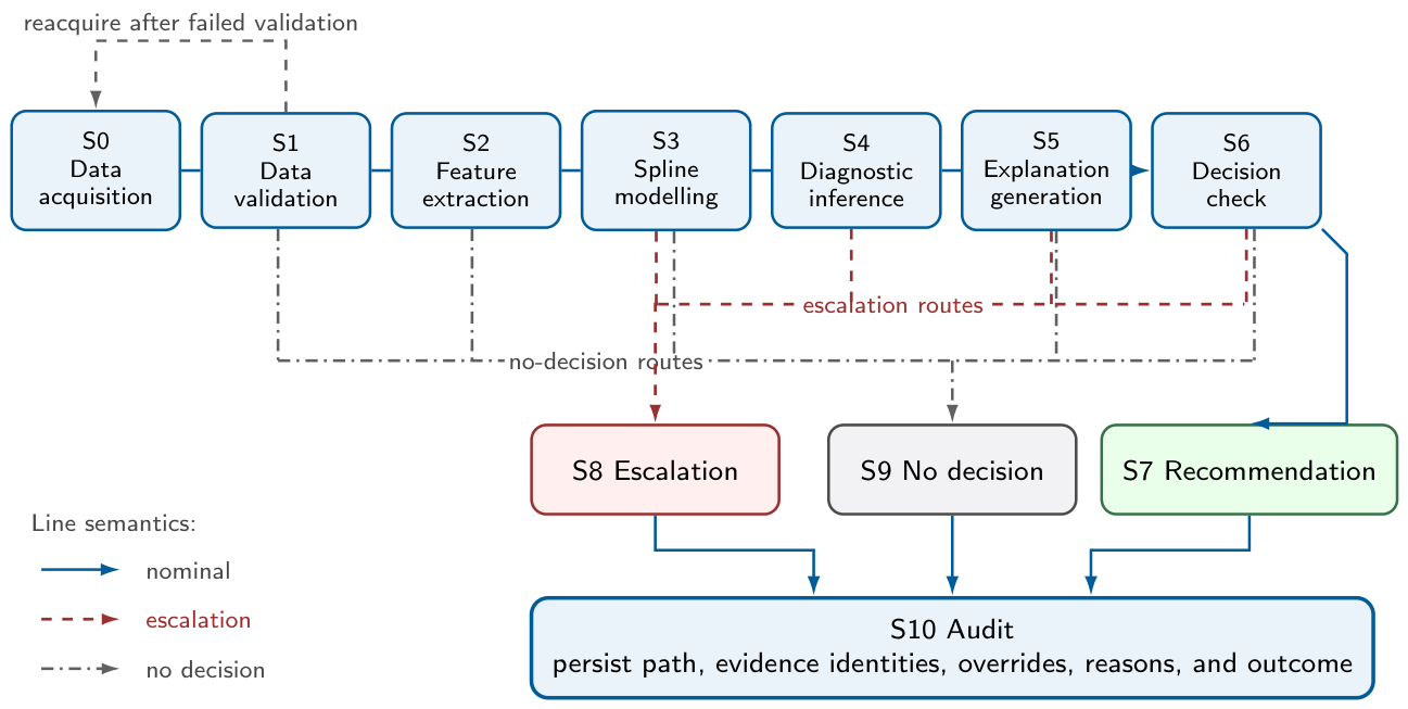
Figure 5.
Audit and deterministic replay contract. One frozen set of persisted artifacts—the EvidenceBundle, routing policy, and configuration—feeds both the original execution and replay under the same deterministic rules. The original execution produces a hash-linked audit chain and a reference signature; replay reconstructs the state path, SafetyGuard overrides, final disposition, and run hash. Equality of these scientific fields yields a verified replay, whereas any mismatch is recorded as an integrity failure.
Figure 5.
Audit and deterministic replay contract. One frozen set of persisted artifacts—the EvidenceBundle, routing policy, and configuration—feeds both the original execution and replay under the same deterministic rules. The original execution produces a hash-linked audit chain and a reference signature; replay reconstructs the state path, SafetyGuard overrides, final disposition, and run hash. Equality of these scientific fields yields a verified replay, whereas any mismatch is recorded as an integrity failure.
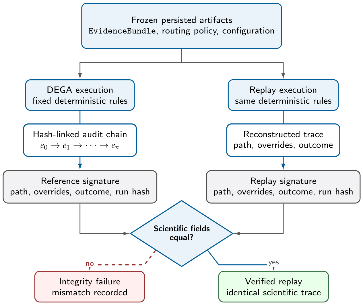
Figure 6.
Acquisition-level classifier performance across 16 dependent assignment views. The left panel shows macro-F1 and the right panel balanced accuracy for LR, RF, and HGB. Each marker represents one class-complete assignment view containing four training and four held-out acquisitions; vertically stacked markers reveal repeated values. Marker shape and fill redundantly identify the classifier, and the black vertical segment with the adjacent number marks the median over the 16 views. LR attains the highest median acquisition-level macro-F1 (1.00), compared with 0.67 for RF and HGB. The views are dependent exhaustive selections from the same eight acquisitions, not independent replications; their spread therefore provides a descriptive summary of the dependent assignment views, while sampling uncertainty requires independent replications.
Figure 6.
Acquisition-level classifier performance across 16 dependent assignment views. The left panel shows macro-F1 and the right panel balanced accuracy for LR, RF, and HGB. Each marker represents one class-complete assignment view containing four training and four held-out acquisitions; vertically stacked markers reveal repeated values. Marker shape and fill redundantly identify the classifier, and the black vertical segment with the adjacent number marks the median over the 16 views. LR attains the highest median acquisition-level macro-F1 (1.00), compared with 0.67 for RF and HGB. The views are dependent exhaustive selections from the same eight acquisitions, not independent replications; their spread therefore provides a descriptive summary of the dependent assignment views, while sampling uncertainty requires independent replications.
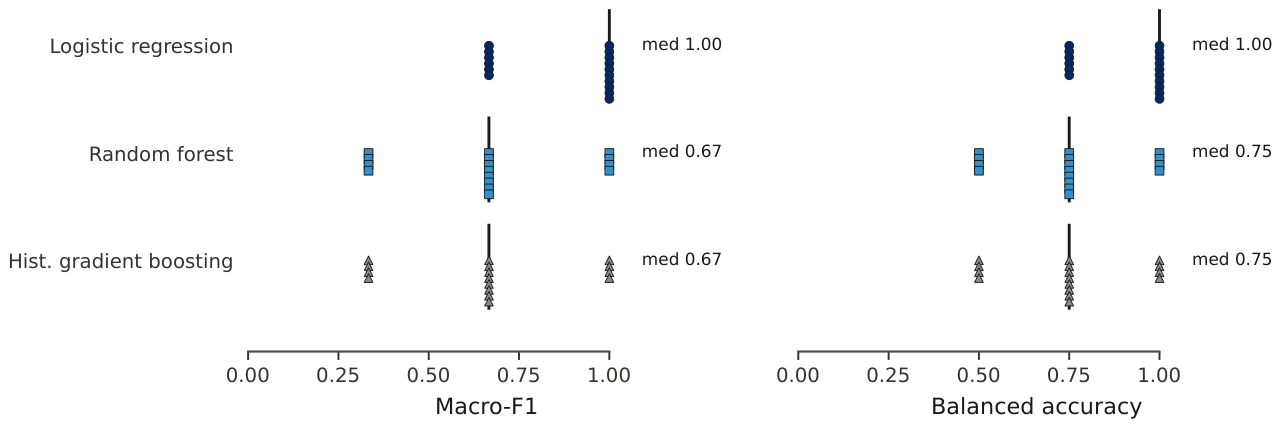
Figure 7.
Window-level versus acquisition-level evaluation of the same fitted models. Each panel corresponds to one classifier. Thin lines pair the window-level and acquisition-level macro-F1 obtained from the same fitted model and assignment view, while the thick black line connects the medians over all 16 views. Window-level medians are similar across classifiers, whereas acquisition-level aggregation separates LR from the two tree-based models. The 100 held-out windows within a view are nested in four held-out acquisitions and are not independent experimental units.
Figure 7.
Window-level versus acquisition-level evaluation of the same fitted models. Each panel corresponds to one classifier. Thin lines pair the window-level and acquisition-level macro-F1 obtained from the same fitted model and assignment view, while the thick black line connects the medians over all 16 views. Window-level medians are similar across classifiers, whereas acquisition-level aggregation separates LR from the two tree-based models. The 100 held-out windows within a view are nested in four held-out acquisitions and are not independent experimental units.
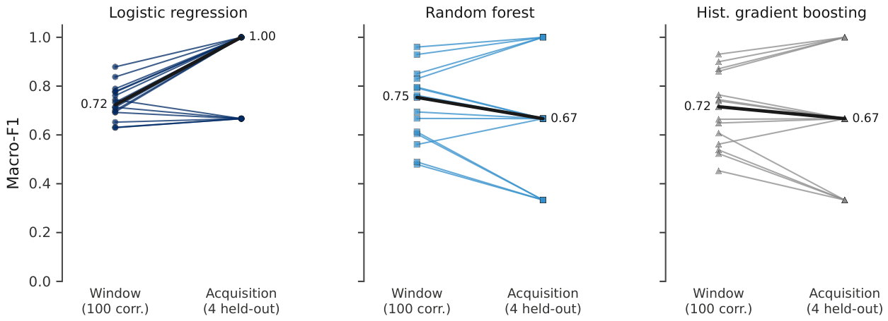
Figure 8.
Scalar spline evidence persisted by ArticleV1. The left panel shows the scalar trend value in all 256 persisted records: 16 assignment views, four held-out acquisitions per view, and four rolling-spline representations. A symmetric-logarithmic axis is used because values span several orders of magnitude and include both signs; vertical jitter within a row is only for visibility. The right panel shows all five descriptors stored for one representative record (A05, healthy_1, rolling smoothing spline), with the numerical values printed directly. No complete trajectory or derivative array was persisted, so the figure deliberately avoids reconstructing a curve. Derivatives refer to ordered window position rather than physical time and must not be interpreted as degradation rates, degradation acceleration, physical fault onset, or remaining useful life.
Figure 8.
Scalar spline evidence persisted by ArticleV1. The left panel shows the scalar trend value in all 256 persisted records: 16 assignment views, four held-out acquisitions per view, and four rolling-spline representations. A symmetric-logarithmic axis is used because values span several orders of magnitude and include both signs; vertical jitter within a row is only for visibility. The right panel shows all five descriptors stored for one representative record (A05, healthy_1, rolling smoothing spline), with the numerical values printed directly. No complete trajectory or derivative array was persisted, so the figure deliberately avoids reconstructing a curve. Derivatives refer to ordered window position rather than physical time and must not be interpreted as degradation rates, degradation acceleration, physical fault onset, or remaining useful life.
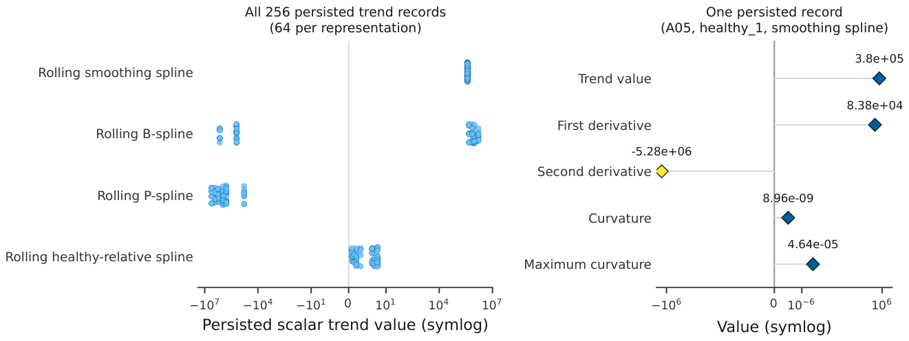
Figure 9.
Resolution and saturation of the DEGA risk components. The left panel gives empirical cumulative distributions over all 768 frozen risk records for classifier uncertainty, Healthy-reference deviation, trend uncertainty, OOD contribution, and their combined risk. The yellow line marks the upper bound 1.0. The right panel shows the number of distinct persisted values for each component on a logarithmic scale. Classifier uncertainty and combined risk retain substantially more resolution than the other components; OOD contribution and trend uncertainty are strongly saturated. Values are displayed exactly as persisted: no component, weight, threshold, or scale was retuned. The combined score is an experimental aggregate used for workflow routing under the configured evidence model. The 768 records are dependent combinations of the same assignment views and acquisitions.
Figure 9.
Resolution and saturation of the DEGA risk components. The left panel gives empirical cumulative distributions over all 768 frozen risk records for classifier uncertainty, Healthy-reference deviation, trend uncertainty, OOD contribution, and their combined risk. The yellow line marks the upper bound 1.0. The right panel shows the number of distinct persisted values for each component on a logarithmic scale. Classifier uncertainty and combined risk retain substantially more resolution than the other components; OOD contribution and trend uncertainty are strongly saturated. Values are displayed exactly as persisted: no component, weight, threshold, or scale was retuned. The combined score is an experimental aggregate used for workflow routing under the configured evidence model. The 768 records are dependent combinations of the same assignment views and acquisitions.
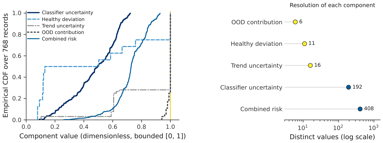
Figure 10.
Global permutation importance for the executed RF model in assignment view A00. All 28 implemented diagnostic features are ordered by their persisted mean decrease in balanced accuracy over 30 permutation repeats. Dark markers show the means and pale markers the individual repeats. Speed-domain amplitude features lead the ranking, but the largest mean decrease is only about 0.06 and most features lie near zero. The ranking is specific to one RF model, one assignment view, and 100 correlated held-out windows; it is neither a universal physical feature ranking nor evidence of causal relevance. Harmonic-amplitude features are absent because they were not implemented in ArticleV1.
Figure 10.
Global permutation importance for the executed RF model in assignment view A00. All 28 implemented diagnostic features are ordered by their persisted mean decrease in balanced accuracy over 30 permutation repeats. Dark markers show the means and pale markers the individual repeats. Speed-domain amplitude features lead the ranking, but the largest mean decrease is only about 0.06 and most features lie near zero. The ranking is specific to one RF model, one assignment view, and 100 correlated held-out windows; it is neither a universal physical feature ranking nor evidence of causal relevance. Harmonic-amplitude features are absent because they were not implemented in ArticleV1.
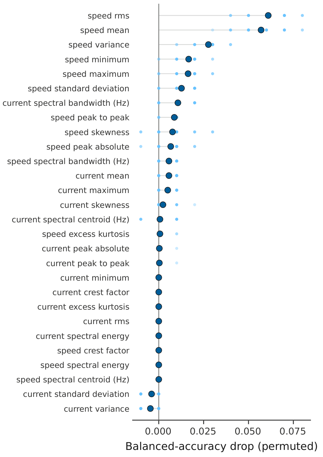
Figure 11.
Stability of the top-10 global explanation across 16 dependent assignment views. The left panel is the complete symmetric matrix of pairwise Jaccard similarity between the top-10 permutation-importance feature sets; the diagonal is the trivial self-similarity of 1.0. The right panel displays the 120 unique off-diagonal pairs as a dot histogram, with the black line marking the median (0.33) and the yellow line the value 1.0 expected for identical sets. No pair yields an identical top-10 set. Because all views reuse the same eight acquisitions and each model is trained on only four acquisitions, the figure characterizes assignment sensitivity in this small case study rather than variability across independent datasets.
Figure 11.
Stability of the top-10 global explanation across 16 dependent assignment views. The left panel is the complete symmetric matrix of pairwise Jaccard similarity between the top-10 permutation-importance feature sets; the diagonal is the trivial self-similarity of 1.0. The right panel displays the 120 unique off-diagonal pairs as a dot histogram, with the black line marking the median (0.33) and the yellow line the value 1.0 expected for identical sets. No pair yields an identical top-10 set. Because all views reuse the same eight acquisitions and each model is trained on only four acquisitions, the figure characterizes assignment sensitivity in this small case study rather than variability across independent datasets.
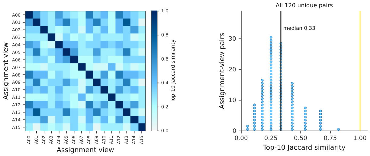
Figure 12.
Terminal outcomes of all 12 representative DEGA executions. Rows are the three persisted article scenarios and columns the four transition policies. Each cell reports the terminal disposition, number of visited states, and whether the SafetyGuard overrode a proposed transition. The static transition-matrix policy escalates in all three scenarios after a nine-state path and one override; the other three policies return no automated recommendation after four states and no override. No execution produces a recommendation. The bracketed EB tags identify the underlying EvidenceBundle hashes: scenarios S01 and S05 share EB1, so the three scenario labels represent only two distinct evidence bundles. These executions demonstrate workflow behavior across the selected scenarios; statistical policy benchmarking requires a broader experimental design.
Figure 12.
Terminal outcomes of all 12 representative DEGA executions. Rows are the three persisted article scenarios and columns the four transition policies. Each cell reports the terminal disposition, number of visited states, and whether the SafetyGuard overrode a proposed transition. The static transition-matrix policy escalates in all three scenarios after a nine-state path and one override; the other three policies return no automated recommendation after four states and no override. No execution produces a recommendation. The bracketed EB tags identify the underlying EvidenceBundle hashes: scenarios S01 and S05 share EB1, so the three scenario labels represent only two distinct evidence bundles. These executions demonstrate workflow behavior across the selected scenarios; statistical policy benchmarking requires a broader experimental design.
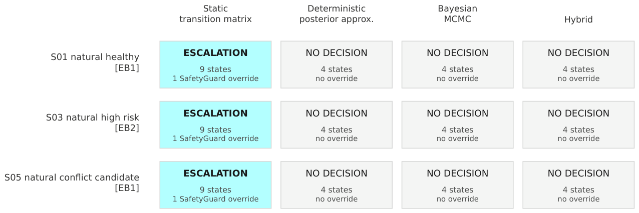
Figure 13.
The two distinct state paths realized by the 12 DEGA executions. Open circles denote intermediate states and filled diamonds terminal states. The solid path, realized by the static transition-matrix policy in three runs, traverses acquisition, validation, feature extraction, spline modelling, inference, explanation, decision check, escalation, and audit. The dashed path, realized by the deterministic posterior-approximation, Bayesian MCMC, and hybrid policies in nine runs, moves from validation directly to no decision and audit. The figure enumerates the complete set of paths observed in the frozen study; the 12 runs are representative workflow executions rather than a sample for statistical inference.
Figure 13.
The two distinct state paths realized by the 12 DEGA executions. Open circles denote intermediate states and filled diamonds terminal states. The solid path, realized by the static transition-matrix policy in three runs, traverses acquisition, validation, feature extraction, spline modelling, inference, explanation, decision check, escalation, and audit. The dashed path, realized by the deterministic posterior-approximation, Bayesian MCMC, and hybrid policies in nine runs, moves from validation directly to no decision and audit. The figure enumerates the complete set of paths observed in the frozen study; the 12 runs are representative workflow executions rather than a sample for statistical inference.
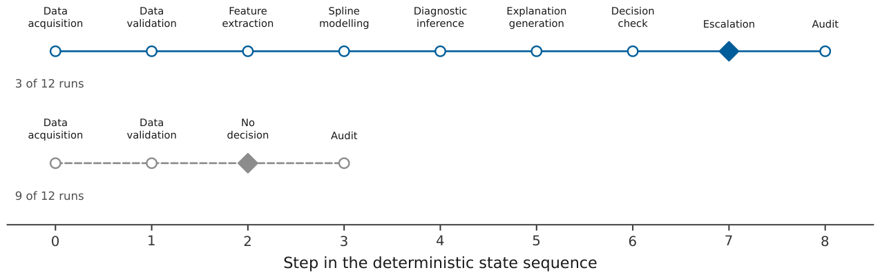
Figure 14.
Evidence hashing, audit-chain integrity, and deterministic replay. Bars show the verified fraction and labels give exact verified/total counts. All 768 persisted EvidenceBundle objects were reconstructed and reloaded with identical scientific hashes. For all 12 representative runs, the audit-event hash linkage was independently recomputed without a break, the persisted audit-valid flag was true, and deterministic replay reproduced the recorded state path, SafetyGuard outcome, and terminal disposition. These checks establish completeness, integrity, and reproducibility of the frozen computation; they do not establish diagnostic accuracy or correctness of the resulting decisions.
Figure 14.
Evidence hashing, audit-chain integrity, and deterministic replay. Bars show the verified fraction and labels give exact verified/total counts. All 768 persisted EvidenceBundle objects were reconstructed and reloaded with identical scientific hashes. For all 12 representative runs, the audit-event hash linkage was independently recomputed without a break, the persisted audit-valid flag was true, and deterministic replay reproduced the recorded state path, SafetyGuard outcome, and terminal disposition. These checks establish completeness, integrity, and reproducibility of the frozen computation; they do not establish diagnostic accuracy or correctness of the resulting decisions.
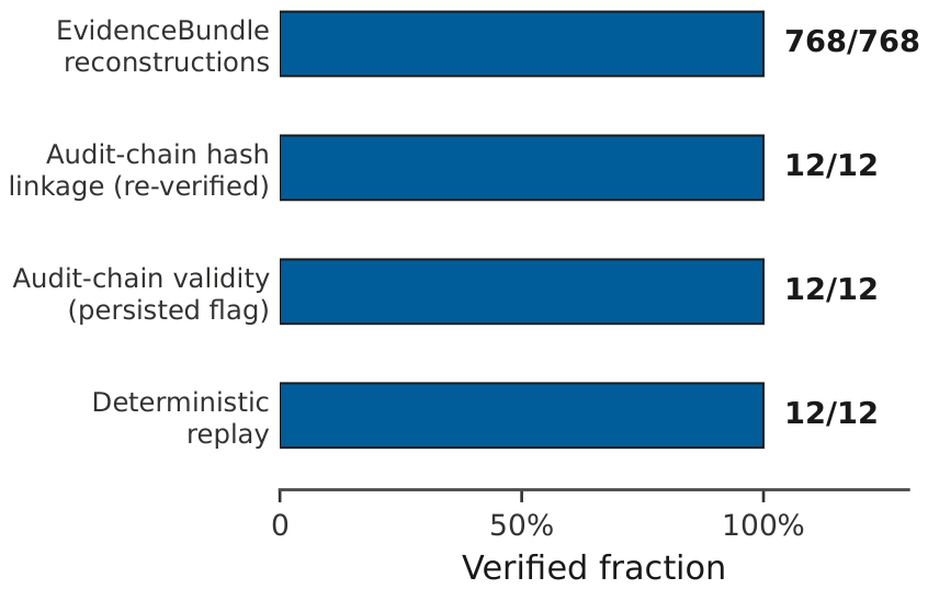

Table 1.
Implemented diagnostic evidence groups. “Admissible interpretation” describes what the feature can support in the present case study; it does not establish a unique causal fault signature.
Table 1.
Implemented diagnostic evidence groups. “Admissible interpretation” describes what the feature can support in the present case study; it does not establish a unique causal fault signature.
| Evidence | Signal property | Admissible interpretation | Governance use |
|---|---|---|---|
| RMS and mean | Overall current or speed level | Supports comparison with the active operating and Healthy references | Retained with acquisition, model, and reference provenance |
| Standard deviation and variance | Within-window variability | Supports an instability interpretation when corroborated by other evidence | Cannot alone authorize a fault recommendation |
| Crest factor and kurtosis | Peak-to-typical ratio and tail behaviour | Supports identification of impulsive or non-Gaussian windows | Used as descriptive evidence requiring corroboration for fault attribution |
| Spectral energy, centroid, bandwidth | Broad frequency-domain distribution | Supports detection of changes in spectral content without assigning a specific harmonic | Prevents unsupported harmonic localization |
| Spline slope and curvature | Geometric change over ordered windows | Supports comparison of local trend shape | Interpreted relative to window order, not physical degradation time |
| Healthy-relative distance | Difference from a training-only reference | Supports an assignment-specific departure statement | Requires verified reference provenance |
Table 2.
Canonical DEGA state dictionary. Every terminal disposition is followed by the explicit audit state.
Table 2.
Canonical DEGA state dictionary. Every terminal disposition is followed by the explicit audit state.
| ID | State | Role |
|---|---|---|
| S0 | Data acquisition | Resolve the persisted acquisition or measurement source. |
| S1 | Data validation | Verify identity, completeness, schema, hashes, and admissibility. |
| S2 | Feature extraction | Represent the case-local feature stage in the execution trace. |
| S3 | Spline modelling | Attach or verify temporal spline evidence. |
| S4 | Diagnostic inference | Consume classifier and acquisition-level evidence. |
| S5 | Explanation generation | Attach available explanation evidence and provenance. |
| S6 | Decision check | Evaluate sufficiency, uncertainty, conflict, and risk inputs. |
| S7 | Recommendation | Issue an admissible diagnostic recommendation. |
| S8 | Escalation | Transfer an ambiguous or high-risk case to human review. |
| S9 | No decision | Refuse automated recommendation when the evidence is insufficient or incompatible. |
| S10 | Audit | Persist the state path, evidence identities, overrides, reasons, and final outcome. |
Disclaimer/Publisher’s Note: The statements, opinions and data contained in all publications are solely those of the individual author(s) and contributor(s) and not of MDPI and/or the editor(s). MDPI and/or the editor(s) disclaim responsibility for any injury to people or property resulting from any ideas, methods, instructions or products referred to in the content. |
© 2026 by the authors. Licensee MDPI, Basel, Switzerland. This article is an open access article distributed under the terms and conditions of the Creative Commons Attribution (CC BY) license (http://creativecommons.org/licenses/by/4.0/).
Copyright: This open access article is published under a Creative Commons CC BY 4.0 license, which permit the free download, distribution, and reuse, provided that the author and preprint are cited in any reuse.


