

Submitted:
17 July 2026
Posted:
20 July 2026
You are already at the latest version
Abstract
Flocculation-sedimentation is a widely used solid-liquid separation process in mineral processing and wastewater treatment, yet its optimization remains challenging due to nonlinear interactions among reagents, solids, and operating conditions. This study presents a statistically rigorous multi-response optimization framework combining HuberT robust regression, canonical analysis, and the Derringer desirability function, and demonstrates its application to coal slurry water treatment as a case study. Coal slurry concentration, polyacrylamide (PAM) dosage, and CaCl₂ concentration were used as factors, with supernatant turbidity and initial settling velocity as responses. A central composite design (20 runs) was employed, and second-order models were fitted via HuberT M-estimation to mitigate the influence of potential outliers. Both the ln-transformed turbidity model (R² = 0.9887) and settling velocity model (R² = 0.9908) showed high significance and predictive capability. Canonical analysis confirmed that the turbidity response surface exhibits a true minimum within the design space, while the settling velocity surface has a saddle-point structure. HuberT weight diagnostics identified no downweighted runs for turbidity and two mildly influential runs for settling velocity, confirming overall data consistency. Multi-response optimization via the Derringer desirability function yielded a combined optimum (coal slurry 25.27 g/L, PAM 5.19 mg/L, CaCl₂ 2.07 g/L; desirability D = 0.8981) with predicted turbidity of 29.21 NTU and settling velocity of 13.26 mm/s. The proposed framework is generalizable to other flocculation-sedimentation systems requiring simultaneous improvement of multiple, often conflicting, process responses.
Keywords:
process optimization
; flocculation-sedimentation
; robust regression
; central composite design
; HuberT M-estimation
; canonical analysis
; Derringer desirability function
; solid-liquid separation
1. Introduction
Coal remains the foundation of China's energy system. In 2024, national raw coal output reached 4.78 billion tonnes, up 1.2% year on year, while the total processing capacity of coal preparation plants exceeded 3.2 billion tonnes, with wet separation accounting for more than 90% of this capacity [1,2]. At this industrial scale, annual coal slurry water discharge exceeds 10 billion cubic meters, and the effectiveness of its treatment directly determines whether preparation plants can achieve closed-loop water circulation and wastewater reduction. Suspended particles in coal slurry water are typically smaller than 0.5 mm, so gravity settling alone is rarely sufficient for effective solid–liquid separation; coagulants and flocculants are required to promote the aggregation of fine particles into larger flocs [3]. As coal mining mechanization has increased, the proportion of high-ash, clay-rich gangue in raw coal has also risen, making the high-ash fine slurry produced by wet coal preparation even harder to settle—a persistent practical challenge for China's coal preparation industry [4]. From an engineering perspective, the effectiveness of coal slurry water treatment depends heavily on reagent type, dosing sequence, and dosage; however, many plants still rely on manual, experience-based dosing, which is subjective and slow to respond, often introducing process fluctuations in both flotation and settling stages [5].
Among current process reagents, polyacrylamide (PAM) and calcium chloride (CaCl2) are a commonly used combination. PAM has long molecular chains that can adsorb simultaneously onto multiple particle surfaces, linking fine flocs into larger aggregates through polymer bridging [6]; the Ca2+ released by CaCl2 compresses the electrical double layer on particle surfaces, reducing electrostatic repulsion between particles and thereby promoting particle approach and destabilization [7]. A number of domestic studies have examined this reagent system. For example, Fan Youlin et al. [8] investigated the effect of CPAM ionicity on the settling behavior of highly argillized coal slurry water, while Wang Lujun et al. [9] synthesized a P(AM-DMDAAC) copolymer from a molecular design perspective and evaluated its flocculation performance on fine kaolinite particles. Overall, the hydration characteristics and electrical double-layer structure of fine particle surfaces are key interfacial factors governing flocculation performance [10,11]. In practice, CaCl2 is typically dosed first to destabilize the particles, followed by PAM for bridging flocculation—an operating logic that is already well established. The real difficulty lies in dose calibration: whether a significant interaction exists between PAM and CaCl2, its direction, and where the optimal ratio lies are questions that single-factor experiments cannot adequately answer. More importantly, reducing supernatant turbidity and increasing settling velocity are not always aligned objectives, and practical optimization often requires a trade-off between clarification performance and processing efficiency.
Response surface methodology (RSM) is well suited to such multi-factor, multi-response optimization problems [12]. Within a relatively limited number of trials, it can estimate not only main effects but also quadratic effects and interactions among factors, and has therefore been widely applied to optimizing coal slurry flocculation and settling processes. Zhao Yang et al. [4], in a review of technologies for treating hard-to-settle coal slurry water, noted that fine-tuned reagent dosing is an important direction for improving settling efficiency. In recent years, researchers have commonly used Box–Behnken designs or central composite designs (CCD), with PAM dosage, pH, and coal slurry concentration as factors and settling velocity or supernatant turbidity as responses, to fit second-order polynomial models. For instance, Mao Xinru et al. [13] carried out a response surface study on coagulation–flocculation settling of tailings coal slurry, while Yao Yuan et al. [14] used RSM to investigate static and dynamic flocculation settling behavior of whole tailings.
The Hansdah group has conducted relatively systematic work on optimizing the settling of coal fine tailings. Focusing on coal fine tailings from an Indian coal preparation plant, they successively applied full factorial designs, central composite rotatable designs, and Box–Behnken designs to analyze the effects of pH, flocculant dosage, and slurry concentration on settling performance [15,16,17,18]. Other studies have combined RSM with desirability functions for simultaneous multi-response optimization; Shi et al. [19] adopted this approach to optimize the settling parameters of ultrafine tailings slurry. Indeed, the statistical framework of RSM is not confined to mineral processing and has also been applied in food processing optimization [20] and agricultural machinery parameter optimization [21], demonstrating its broad applicability. Nevertheless, for coal slurry flocculation systems specifically, model interpretation must still be grounded in particle surface properties, reagent mechanisms, and settling dynamics, rather than remaining at the level of statistical fitting alone.
However, most existing response surface studies estimate regression coefficients using ordinary least squares (OLS), which is sensitive to outliers. In coal slurry settling experiments, uneven instantaneous distribution of suspended particles, bubble interference, sampling disturbance, and manual reading error can all cause individual data points to deviate from the overall trend. If such points are included in an OLS fit with equal weight, the model coefficients and the shape of the response surface can be distorted. HuberT M-estimation robust regression offers a more reliable alternative: through an iterative process, it adaptively reduces the weight of outlying points while retaining all original data, thereby limiting the influence of outlying observations on parameter estimation [22]. Although well established in robust statistics, this method has seen relatively limited application in response surface modeling of coal slurry flocculation.
Another gap concerns the fact that most existing studies still focus on single-response optimization, emphasizing either turbidity reduction or settling velocity improvement, with relatively few studies genuinely treating both as simultaneous dual-response objectives. Moreover, some studies proceed directly to numerical optimization after obtaining a regression model, without further conducting canonical analysis to determine the nature of the stationary point on the response surface. This step may appear to be a modeling detail, but it is in fact critical: it helps distinguish a genuine interior extremum of the response surface from a boundary solution found by the optimization algorithm at the edge of the design space. Without this check, the so-called “optimal process parameters” may simply reflect a bounded search result rather than a true interior optimum of the response surface itself.
Based on the issues outlined above, this study uses coal slurry mass concentration, PAM mass concentration, and CaCl2 mass concentration as three factors, and turbidity and settling velocity as dual response indicators, to establish a second-order response surface model using a central composite design combined with HuberT robust regression. The study includes: evaluating model fit quality through analysis of variance; interpreting the main effects and interaction effects of the factors using response surface and contour plots; using canonical analysis to determine the nature of the stationary points; and finally applying the Derringer desirability function to achieve simultaneous multi-response optimization of turbidity and settling velocity [23]. By combining more robust parameter estimation with more complete response surface diagnostics within the traditional response surface optimization framework, this study aims to provide a more reliable modeling basis for the quantitative control of reagent dosing in coal slurry flocculation processes.
2. Materials and Methods
2.1. Properties of the Coal Slurry at the Thickener Feed Inlet
The coal slurry water used in this study was collected from the No. 8 Mine coal preparation plant of Pingmei Shenma Energy and Chemical Group, China. Samples were taken from the coal slurry water formed by the combined tailings of the flotation cell and the gravity separator prior to entering the thickener. Samples were vacuum-filtered, dried, thoroughly homogenized, and stored in sealed bags for subsequent property analysis and settling tests. Characterizing the properties of the feed coal slurry is a prerequisite for improving its settling performance; accordingly, prior to testing, the calorific value, functional groups, mineral phases, and particle size distribution of the coal sample were analyzed.
2.1.1. Calorific Value of the Coal Sample
An oxygen bomb calorimeter (model 5E-AC8018, Kaiyuan Instruments) was used to measure the calorific value of the coal sample, and a muffle furnace was used to determine the ash content, as shown in Table 1. The sample had a dry-basis ash content of 39.00%, which, according to the Chinese national standard GB/T 15224.1 (Classification for Quality of Coal—Part 1: Ash Yield), falls within the extra-high-ash range (Ad > 34.00%); the dry-basis higher heating value was 16,409 J/g, which, according to GB/T 15224.3 (Classification for Quality of Coal—Part 3: Calorific Value), falls within the low-calorific-value range, well below typical steam coal levels. This combination of elevated ash content and reduced calorific value is highly consistent with the sample's process origin: both flotation and gravity separation are processes for concentrating combustible organic matter, and their tailings, as low-quality by-products discharged after separation, have had most of their combustible fraction removed while mineral impurities are relatively enriched, giving rise to the characteristic pattern of markedly elevated ash content and markedly reduced calorific value.
Note: ad, air-dried basis; d, dry basis; daf, dry ash-free basis.
2.1.2. Functional Group Analysis of the Coal Sample
To clarify the mineral composition and surface functional groups of the solid particles in the coal slurry water system, the sample was analyzed by Fourier-transform infrared (FTIR) spectroscopy using a NICOLET38 spectrometer over a scanning range of 400–4000 cm−1. As shown in Figure 1 and Table 2, three characteristic sharp peaks appear in the 3600–3700 cm−1 region, a typical fingerprint of hydroxyl stretching vibrations in kaolinite-group minerals; this is corroborated by the Al—OH bending vibration peak at 914 cm−1. The strongest absorption peak in the entire spectrum occurs at 1032 cm−1 (prominence 76.12), assigned to the Si—O—Si framework stretching vibration of layered silicates. Taken together, these characteristic peaks confirm that the dominant mineral phase in the sample is kaolinite with a relatively well-preserved layer structure. In addition, weak peaks at 2924 cm−1 and 1433 cm−1 correspond to aliphatic —CH2—/—CH3 vibrations, indicating a small amount of residual organic matter; several absorption peaks in the low-wavenumber fingerprint region (400–800 cm−1) further confirm the layered silicate structure of kaolinite. These results indicate that the abundant Si—O and Al—OH active sites on the clay mineral surface can, on one hand, anchor the amide groups of the nonionic PAM chains through hydrogen bonding, providing an interface for adsorption bridging, and on the other hand, form an important physicochemical basis for charge neutralization and double-layer compression by Ca2+.
2.1.3. Phase Analysis of the Coal Sample
To further verify the mineral phase composition, the sample was analyzed by X-ray diffraction (XRD) using a Shimadzu XRD-6000 diffractometer. As shown in Figure 2, the characteristic diffraction peaks detected in the sample match two reference phases in the ICDD-PDF database: quartz (SiO2, ICDD PDF#79-1906) and kaolinite (Al2Si2O5(OH)4, corresponding to ICDD PDF#78-2109 and PDF#78-1996). The characteristic peaks of kaolinite and quartz both correspond clearly in the pattern, indicating that these two minerals constitute the dominant solid-phase components of the sample. This result provides direct support for the discussion of the material basis of the flocculation mechanism in Section 4.2.3.
2.1.4. Particle Size Distribution Analysis of the Coal Sample
Particle size was measured using a Winner2308A laser particle size analyzer with a measurement range of 0.01–2000 μm, water as the dispersion medium, and a sample concentration of approximately 6.57%. As shown in Table 3 and Table 4 and Figure 3, particle sizes are mainly distributed between 0.45 and 81 μm, and the volume distribution is multimodal, with peaks at approximately 1.13 μm, 3.30 μm, and 8.23 μm, indicating that the sample consists of a mixture of fine particles (clay mineral microparticles) and relatively coarser particles (coal fines and aggregates), consistent with the solid-phase properties of coal slurry water. Size-interval statistics show that the 1–5 μm interval has the largest volume fraction, 44.30%, representing the dominant size range of the sample. The key characteristic values are D10 = 1.020 μm, D50 = 4.059 μm, D90 = 13.944 μm, and Span = 3.18, indicating that the sample is overall in the fine particle range with a broad and relatively poor distribution uniformity. The specific surface area (S/V) of the sample is 22,935.040 cm2/cm3, a relatively high value that has an important influence on the subsequent adsorption-bridging efficiency of the flocculation reagents (PAM, CaCl2) at the particle surface, providing a particle-size-level basis for the discussion of the flocculation mechanism in Section 4.2.
2.2. Materials
2.2.1. Reagents
The flocculant used in this study was nonionic polyacrylamide (NPAM), analytical grade, with a molecular weight of approximately 10 million; the coagulant was anhydrous calcium chloride, also analytical grade. Prior to use, the flocculant was prepared as a 0.1% (w/v) aqueous solution and the coagulant as a 5% (w/v) aqueous solution.
2.2.2. Equipment
500 mL settling cylinders, beakers, glass rods, pipette guns, test tubes, pipettes, a magnetic heating stirrer, a video camera, a camera tripod, and a Leici WZS-188 turbidimeter.
2.3. Settling Test Procedure
Settling tests were carried out in 500 mL settling cylinders. The procedure was as follows: a weighed amount of sample was placed in a settling cylinder, and clarified process water was added to reach the desired concentration, followed by thorough mixing to ensure uniform dispersion of the tailings particles in the water. A measured amount of coagulant was then added and stirred for a set period, after which the required flocculant was added; the suspension was stirred three times and then left to stand, while the descent of the clarification interface was recorded from that point. The test ended once the clarification interface had stabilized. Settling performance was evaluated using the initial settling velocity and supernatant turbidity as indicators. The initial settling velocity was calculated from the change in the position of the clarification interface over time, following the Chinese national standard GB/T 18712–2002 (Test Method for Performance of Flocculants for Coal Preparation). Supernatant turbidity was measured three times using a Leici WZS-188 turbidimeter and averaged.
2.4. Experimental Design
This study used a central composite design (CCD) with three factors—coal slurry mass concentration, PAM mass concentration, and CaCl2 mass concentration—each examined at five levels, with supernatant turbidity and initial settling velocity as the response indicators. A rotatable CCD was adopted, with the axial arm length set to the standard rotatable value α = 1.682 for three factors. A total of 20 runs were arranged, comprising 8 cube points, 6 axial points, and 6 replicated center points; the replicated center points were used to estimate pure error and assess model lack of fit. The factor levels are given in Table 5.
Factor coding, generation of the experimental design, fitting of the second-order response surface models, analysis of variance, canonical analysis, and multi-response optimization were all carried out using custom analysis scripts written in Python (version 3.12): the design matrix generation and numerical computations were implemented with NumPy (version 2.4); the HuberT robust regression fitting of the second-order polynomial models used the robust module of statsmodels (version 0.14); the eigenvalue decomposition of the Hessian matrix for analysis of variance and canonical analysis used the linear algebra and statistics modules of SciPy (version 1.17); and response surface visualization was implemented with Matplotlib (version 3.10). In contrast to the ordinary least squares estimation adopted by default in conventional response surface analysis software, this study implements robust regression fitting in Python to better control the influence of outlying observations on the model parameters. The generated CCD experimental design and the measured response values are shown in Table 6.
The basic idea of HuberT M-estimation is to adaptively downweight observations with large residuals within the least-squares framework, thereby limiting the excessive influence of individual anomalous observations on the regression coefficients, while treating observations with small residuals in the same way as ordinary least squares.
Specifically, let ui denote the standardized residual of the i-th observation; the Huber loss function is defined as ρ(ui) = ui2/2 when |ui| ≤ c, and ρ(ui) = c(|ui| − c/2) when |ui| > c, where c is a tuning constant; this study adopts the statsmodels default value of c = 1.345 (corresponding to approximately 95% asymptotic relative efficiency under the normal distribution assumption). The corresponding weight function is w(ui) = 1 when |ui| ≤ c, and w(ui) = c/|ui| when |ui| > c. The regression coefficients are solved through Iteratively Reweighted Least Squares (IRLS): each iteration first fits a weighted least-squares estimate using the current weights, then updates the weights based on the new residuals, and the process continues until the weights converge (convergence is assessed by the change in weights, with a maximum of 200 iterations in this study).
3. Results
3.1. Model Fitting and Analysis of Variance
For the turbidity response, preliminary diagnostics revealed a degree of variance heterogeneity in the raw data; Y1 was therefore natural-log transformed before fitting the response surface model. The analysis of variance results for the ln(Y1) model and the raw Y2 model are shown in Table 7 and Table 8, respectively.
For the turbidity model ln(Y1), the overall regression was highly significant (F = 97.14, p < 0.0001). The model's R2, Adj-R2, and Pred-R2 were 0.9887, 0.9785, and 0.9133, respectively, with a difference between Pred-R2 and Adj-R2 of 0.0652; the Adequate Precision was 32.50 and the CV was 1.30%. These metrics indicate a stable model fit with good predictive capability.
For the settling velocity model Y2, the overall regression was likewise highly significant (F = 119.94, p < 0.0001). This model had R2 = 0.9908, Adj-R2 = 0.9826, Pred-R2 = 0.9315, Adequate Precision = 47.12, and CV = 6.99%. These statistics indicate that the model adequately explains the variation in settling velocity.
It should be noted that the lack-of-fit terms for both models reached statistical significance (ln(Y1): p = 0.0069; Y2: p = 0.0095). At the same time, the pure error from the replicated center-point runs was small in both cases, 0.0014 and 0.1262, respectively.
3.2. Regression Equations and Significance Analysis
Equations (1) and (2) give the coded-form regression equations for turbidity ln(Y1) and settling velocity Y2, respectively, where A, B, and C denote the coded values of coal slurry mass concentration, PAM mass concentration, and CaCl2 mass concentration, over the design range of −1.682 to +1.682.
In the turbidity ln(Y1) model, the linear terms for PAM mass concentration (B, p < 0.0001) and coal slurry mass concentration (A, p = 0.0126) were significant, while CaCl2 mass concentration (C, p = 0.6806) was not significant. The negative coefficient of the B term indicates that, within a certain range, increasing PAM dosage helps reduce turbidity. The quadratic terms A2, B2, and C2 were all significant (p < 0.002 in each case), with B2 showing the largest F value (681.40), indicating a very strong nonlinear effect of PAM dosage on turbidity. Among the interaction terms, AB was significant (p = 0.0030), while AC (p = 0.6628) and BC (p = 0.2142) were not.
In the settling velocity Y2 model, the linear terms for coal slurry mass concentration (A, p < 0.0001) and PAM mass concentration (B, p < 0.0001) were both highly significant, with positive coefficients, the A term having a coefficient of 2.2635. The linear term for CaCl2 mass concentration was not significant (C, p = 0.9168), but its quadratic term C2 was highly significant (p < 0.0001, F = 151.35). In addition, all three interaction terms—AB, AC, and BC—reached significance (AB: p < 0.0001, SS = 21.57; AC: p = 0.0013; BC: SS = 28.75), indicating that settling velocity is strongly influenced by the synergistic action of multiple factors.
3.3. Response Surface and Interaction Analysis
For the turbidity response, ln(Y1) first decreases and then increases as PAM concentration rises, with the response surface overall exhibiting a concave shape (Figure 4). A significant interaction exists between coal slurry concentration and PAM concentration (AB, p = 0.0030): at higher coal slurry concentrations, the reduction in turbidity produced by increasing PAM dosage is more pronounced. In contrast, the interaction between coal slurry concentration and CaCl2 concentration is not significant (AC, p = 0.6628, Figure 5), nor is the interaction between PAM concentration and CaCl2 concentration (BC, p = 0.2142, Figure 6); the contour lines in both cases run essentially parallel to the CaCl2 axis, consistent with the statistical test results.
For the settling velocity response, increases in both coal slurry concentration and PAM concentration promote settling velocity, and their interaction is highly significant (AB, p < 0.0001, SS = 21.57, Figure 7). The interaction between coal slurry concentration and CaCl2 concentration is also significant (AC, p = 0.0013), with the response surface exhibiting a saddle-like shape (Figure 8). The interaction between PAM concentration and CaCl2 concentration is likewise strong (BC, SS = 28.75, Figure 9); when both are increased simultaneously, the improvement in settling velocity is more pronounced.
3.4. Robust Regression Diagnostics
To further verify model reliability, measured-versus-predicted plots, residual plots, and robust weight distribution plots were prepared for both models (Figure 10 and Figure 11). The specific weight assigned to each experimental point is listed in Table 9.
For the turbidity model ln(Y1), measured and predicted values are generally distributed close to the 1:1 diagonal (R2 = 0.9887, Figure 10a), and the residuals show no obvious systematic trend (Figure 10b). The robust weighting results show that all 20 experimental points retained a weight of 1.0000, with none falling below the downweighting threshold of 0.85 (Figure 10c), indicating good overall consistency in the turbidity data with no observations markedly deviating from the general trend.
The settling velocity model Y2 also shows a good fit, with measured and predicted values in close agreement (R2 = 0.9908, Figure 11a) and a relatively uniform residual distribution with no obvious heteroscedasticity (Figure 11b). In terms of weighting, only run 6 (measured settling velocity 4.593 mm/s, weight 0.7961) and run 10 (measured settling velocity 7.406 mm/s, weight 0.7221) were downweighted (Figure 11c).
3.5. Multi-Response Optimization
Multi-response optimization was carried out using the Derringer desirability function. Turbidity was treated as “smaller-the-better” and settling velocity as “larger-the-better”. In this study, the importance weights for the two response parameters (turbidity and sedimentation velocity) were set equal (r1 = r2 = 1), thereby simplifying the combined objective function into a geometric mean form.
In this study, the importance weights for the two response parameters (turbidity and sedimentation velocity) were set equal (r1 = r2 = 1), thereby simplifying the objective function to a geometric mean form: D = d1 × d2 (3). This indicates that the model assigns equal weight to both response objectives during optimization without prioritizing either. If distinct priorities exist between turbidity control and sedimentation efficiency in subsequent process applications, the objective function can be reweighted by adjusting the values of ri to reflect these specific engineering considerations.
A 100 × 100 × 100 grid search was performed within the coded space [−1.682, 1.682]3, and the resulting optimization outcomes are summarized in Table 10.
The overall desirability function reaches its maximum, D = 0.8981, at the coded point A = 0.5267, B = 0.5946, C = 1.6820. This point corresponds to actual process conditions of coal slurry mass concentration 25.27 g/L, PAM mass concentration 5.19 mg/L, and CaCl2 mass concentration 2.07 g/L. Under these conditions, the model predicts a turbidity of 29.21 NTU and a settling velocity of 13.26 mm/s.
Single-objective optimization shows that if turbidity minimization alone is pursued, the optimal conditions are a coal slurry concentration of 19.15 g/L, PAM concentration of 4.31 mg/L, and CaCl2 concentration of 1.37 g/L, giving a predicted turbidity of 21.96 NTU. If settling velocity maximization alone is pursued, the optimum instead lies in a higher-concentration region, namely a coal slurry concentration of 36.82 g/L, PAM concentration of 7.36 mg/L, and CaCl2 concentration of 2.07 g/L, giving a predicted settling velocity of 25.07 mm/s. The clear divergence between these two single-objective optima indicates that low turbidity depends more on moderately low coal slurry concentration and PAM dosage, whereas high settling velocity requires all three factors to be at relatively high levels simultaneously.
3.6. Canonical Analysis
To determine the nature of the stationary point of each second-order response surface, canonical analysis was performed on the turbidity ln(Y1) and settling velocity Y2 models. The quadratic coefficient (Hessian) matrix was constructed and its eigenvalues computed to determine whether each stationary point is an extremum or a saddle point. The results are shown in Table 11.
The stationary point of the turbidity model ln(Y1) has coded coordinates A = −0.090, B = 0.146, C = −0.074, which lie within the design space [−1.682, 1.682]3. The three eigenvalues of the corresponding Hessian matrix are λ1 = 0.051, λ2 = 0.146, and λ3 = 0.315, all positive.
The stationary point of the settling velocity model Y2 has coded coordinates A = −14.523, B = −10.387, C = 11.317, well outside the design space [−1.682, 1.682]3. Its Hessian eigenvalues are λ1 = −1.093, λ2 = 0.050, and λ3 = 1.963, with inconsistent signs.
4. Discussion
4.1. Model Fit Quality and Methodological Considerations
This study combined a central composite design with HuberT M-estimation robust regression to establish second-order response surface models for turbidity ln(Y1) and settling velocity Y2 during coal slurry flocculation. Both models show high coefficients of determination (ln(Y1): R2 = 0.9887, Adj-R2 = 0.9785; Y2: R2 = 0.9908, Adj-R2 = 0.9826), with the difference between Pred-R2 and Adj-R2 below 0.2 in both cases. The Adequate Precision values for the two models are 32.50 and 47.12, respectively, well above the commonly used threshold of 4. Overall, the models fit the experimental data well and also demonstrate strong predictive capability.
One result requiring careful interpretation is that the lack-of-fit terms for both models are statistically significant (ln(Y1): p = 0.0069; Y2: p = 0.0095). This does not necessarily mean the models are unusable. As the analysis of variance shows, the pure error from the replicated center-point runs is very small (0.0014 and 0.1262, respectively); when pure error is very small in the denominator, the lack-of-fit F value can be amplified. Similar situations are commonly observed in response surface studies: when replicate precision is very high, a lack-of-fit test may still return a significant result even though the model has captured the main response pattern (Myers & Montgomery, 2009) [12]. Taking R2, Pred-R2, and Adequate Precision together, the models in this study remain suitable for response prediction and process optimization. It should be noted that this robustness conclusion directly addresses an issue raised in the Introduction: existing response surface studies commonly rely on OLS estimation, which is sensitive to anomalous observations; by adopting HuberT robust regression in this study, the adaptability of the model estimates to potential fluctuations was verified even though the data quality was generally good with no severe outliers, providing methodological assurance for future replicate experiments that may involve measurement error.
4.2. Mechanisms Underlying the Effects of Each Factor on Flocculation Performance
4.2.1. Dominant Role of PAM in Turbidity Reduction and the Restabilization Effect
In the turbidity model, the linear coefficient of PAM mass concentration (term B) is negative and highly significant (p < 0.0001), and its quadratic term B2 has the largest F value of all effect terms (681.40). This indicates that moderately increasing PAM dosage does markedly reduce turbidity; however, once dosage continues to rise beyond the appropriate range, turbidity rebounds. Canonical analysis supports this interpretation: the turbidity response surface has a genuine interior minimum within the design space (stationary point at coded coordinates A = −0.090, B = 0.146, C = −0.074), and all three Hessian eigenvalues are positive, indicating a classic bowl-shaped surface. This determination relies on canonical analysis rather than on numerical optimization results alone: as noted in the Introduction, without canonical analysis, an “optimum” obtained from a grid search may simply be a bounded-search solution found at the edge of the design space, offering no guarantee that a genuine extremum exists within the response surface. In this case, all three Hessian eigenvalues are positive, confirming that the turbidity response surface does indeed contain a genuine interior minimum rather than merely a boundary-search artifact, underscoring why the canonical analysis step should not be omitted in response surface studies.
This nonlinear behavior is consistent with the classical mechanism of “restabilization due to polymer overdosing” in flocculation (Gregory & Barany, 2011) [6]. At an appropriate dosage, PAM chains promote particle aggregation through adsorption and bridging, reducing supernatant turbidity; but when PAM is overdosed, particle surfaces may become covered by a near-saturated polymer adsorption layer, producing steric repulsion. Effective particle collision and aggregation are then hindered, and some previously formed flocs may redisperse, ultimately manifesting as a rebound in turbidity. In practice, therefore, more PAM is not always better; dosage should be controlled within a relatively well-defined optimal window.
4.2.2. Synergistic Mechanism of the Three Factors on Settling Velocity
Unlike the turbidity response, canonical analysis of the settling velocity Y2 model shows that its stationary point (A = −14.523, B = −10.387, C = 11.317) lies outside the design space, with Hessian eigenvalues of inconsistent sign (λ1 = −1.093, λ2 = 0.050, λ3 = 1.963). This indicates that the stationary point is a saddle point rather than a maximum or minimum within the design range. In other words, within the concentration ranges examined here, settling velocity has not yet reached a clear saturation region or inflection point and continues to increase as factor levels rise. This result further confirms the methodological value of canonical analysis: relying on numerical optimization alone, without canonical analysis, could easily lead to mistaking this boundary solution for a genuine interior maximum of the response surface, resulting in an incorrect judgment about whether settling velocity has reached its limit. In this case, the saddle-point determination clearly indicates that this boundary solution merely reflects the search boundary of the current design space and does not imply that settling velocity has saturated.
All three interaction terms—AB, AC, and BC—are significant, with the PAM–CaCl2 interaction (BC, SS = 28.75) showing the largest effect size. This synergy can be understood mechanistically: high-molecular-weight PAM forms bridges among multiple particles through its long chain structure, enlarging floc size and accelerating gravity settling, while the Ca2+ released by CaCl2 compresses the electrical double layer at the particle surface, weakening electrostatic repulsion between particles and thereby creating more favorable conditions for PAM chain adsorption and bridging (Bolto & Gregory, 2007) [7]. Thus, when PAM and CaCl2 act together, their effects are not simply additive; rather, charge regulation and bridging flocculation become coupled, which explains why the BC term shows the strongest effect.
By contrast, the main effect of CaCl2 and its related interaction terms in the turbidity model are not significant (AC: p = 0.6628; BC: p = 0.2142), indicating that under the present experimental conditions, CaCl2 contributes little directly to turbidity reduction. However, in the settling velocity model, the quadratic term for CaCl2, C2, is highly significant (p < 0.0001, F = 151.35), suggesting that its role is expressed mainly in combination with other factors. In other words, increasing CaCl2 concentration alone may not markedly improve clarification, but in combination with PAM it can enhance settling performance by improving bridging efficiency and floc stability.
These results show that the three factors do not act identically on the two response indicators. Turbidity control depends more on fine adjustment of PAM dosage, particularly through its linear and quadratic terms, while improving settling velocity depends more on the synergy among multiple factors, especially the PAM–CaCl2 ratio. For practical process operation, if the objective favors clarity of the effluent, priority should be given to controlling the appropriate PAM dosage; if the objective favors processing efficiency, the coal slurry concentration, PAM, and CaCl2 should be optimized synergistically.
4.2.3. Material Basis of the Flocculation Mechanism
Section 4.2.1 and Section 4.2.2 have largely clarified the two mechanistic lines of PAM adsorption bridging and Ca2+-induced double-layer compression, but this discussion has relied mainly on statistical evidence derived from the response surface models; whether the raw material's own physicochemical properties can support these inferences has not been directly addressed. The mineral phase, functional group, and particle size characterizations provide exactly this material-level evidence.
The FTIR and XRD analyses consistently show that the solid-phase components of the sample are mainly kaolinite and quartz. Kaolinite is a 1:1-type layered silicate mineral whose layer structure consists of silica tetrahedral sheets and alumina octahedral sheets connected by hydrogen bonds; broken edge surfaces of the layers expose abundant Al—OH and Si—OH active sites, while the layer surface is dominated by the Si—O—Si framework. These surface functional groups readily undergo protonation/deprotonation in aqueous environments, giving the particle surface a degree of negative charge. Because the PAM used in this study is nonionic, its molecular chain carries no charge and cannot adsorb directly onto the particle surface through electrostatic interaction; its adsorption-bridging mechanism instead relies mainly on hydrogen bonding between the amide groups (—CONH2) on the chain and the Al—OH and Si—OH active sites on the mineral surface. The nonionic PAM chain anchors to adjacent particle surfaces through multiple hydrogen bonds and bridges them via its long-chain span, forming larger flocs—a process governed mainly by chain conformation and adsorption density rather than by surface charge.
Precisely because nonionic PAM lacks charge-neutralization capability, the negative surface charge of the clay minerals and the resulting electrical double-layer structure in this system are regulated mainly by CaCl2, which is the material basis for the pronounced PAM–CaCl2 synergy discussed in Section 4.2.2: on one hand, Ca2+ preferentially adsorbs onto the negatively charged sites on the kaolinite surface, compressing the double-layer thickness and reducing the electrostatic repulsion potential between particles, thereby creating more favorable conditions for multi-point hydrogen-bond adsorption of nonionic PAM chains; on the other hand, Ca2+ may also undergo ion–dipole coordination with the partially negatively charged carbonyl oxygen of the PAM amide group, forming a cationic bridging structure of “mineral surface—Ca2+—PAM amide group” that reinforces floc formation together with the long-chain physical bridging of PAM itself. This dual mechanism explains why increasing CaCl2 concentration alone has limited effect on turbidity improvement (as noted in Section 4.2, the AC and BC terms are not significant in the turbidity model)—because CaCl2 lacks the spatial bridging capability provided by PAM chains and cannot independently form large flocs—while in the settling velocity model, CaCl2 requires synergy with PAM to exert its full effect, precisely because the two perform two mutually irreplaceable functions: charge regulation and physical bridging.
The particle size distribution results further refine this mineralogical picture at the physical level. The sample's particle size is dominated by the 1–5 μm interval (44.30%), with a median size D50 = 4.059 μm and a relatively high specific surface area (S/V) of 22,935.040 cm2/cm3. A high specific surface area means significantly more adsorption sites per unit mass, providing a physical explanation for the very strong nonlinear effect of the PAM quadratic term noted in Section 4.2.1 (F = 681.40): a system dominated by fine particles is more sensitive to changes in PAM dosage, and once the adsorption saturation threshold is exceeded, a large number of fine particle surfaces simultaneously develop steric repulsion layers, making the restabilization effect correspondingly easier to observe.
In addition, the particle size distribution is multimodal, with peaks at approximately 1.13 μm, 3.30 μm, and 8.23 μm, indicating that the sample is composed of a mixture of fine particles (mainly clay mineral microparticles) and relatively coarser particles (coal fines and aggregates). Fine particles have a larger specific surface area and higher surface charge density, and hence stronger double-layer repulsion, making them more dependent on the charge regulation provided by CaCl2 to achieve effective aggregation; the coarser coal fine aggregates settle faster on their own and depend less on CaCl2. This particle-size differentiation corresponds to the statistical result in Section 4.2.2 that the PAM–CaCl2 interaction is the strongest—a mixed system dominated by fine particles objectively requires the synergy of both charge neutralization and adsorption bridging to achieve adequate flocculation.
4.3. Methodological Value of Robust Regression
The HuberT robust regression diagnostics show that no points were downweighted in the turbidity model (0 out of twenty), compared with two out of twenty in the settling velocity model, the lowest weight in the latter falling to 0.7221. This result indicates that both the turbidity and settling velocity data in this study show good overall consistency; the value of robust regression here lies more in its adaptive capacity to identify and guard against potential outliers than in correcting for a large number of anomalous observations actually present in this dataset.
Without discarding any raw observations, HuberT regression provides an adaptive downweighting mechanism that can reduce the influence of potential outliers on parameter estimation when such points occur. In this study, only run 6 (weight 0.7961) and run 10 (weight 0.7221) in the settling velocity model were moderately downweighted, while the turbidity model showed no downweighted points at all, indicating generally high data quality. The robust regression strategy adopted here retains all experimental information while providing adaptive protection against potential anomalous fluctuations, giving it good methodological value [21].
4.4. Engineering Significance of Multi-Response Optimization
Simultaneous multi-response optimization of turbidity and settling velocity using the Derringer–Suich desirability function reveals a degree of conflict between minimizing turbidity and maximizing settling velocity. The turbidity-optimal solution corresponds to a moderately low coal slurry concentration (19.15 g/L) and PAM dosage (4.31 mg/L), whereas the settling-velocity-optimal solution requires all three factors to approach the upper limit of the design space (coal slurry 36.82 g/L, PAM 7.36 mg/L, CaCl2 2.07 g/L). This difference arises fundamentally from the distinct behavior of the two responses: PAM exerts a pronounced nonlinear extremum effect on turbidity, causing turbidity to rebound due to restabilization beyond the appropriate range, whereas settling velocity, within the range examined here, continues to increase as factor levels rise. This result echoes a gap noted in the Introduction: most existing studies still focus on single-response optimization, whereas this study uses the Derringer desirability function to simultaneously account for both turbidity and settling velocity, offering a dual-response simultaneous optimization scheme that more closely reflects actual production requirements in coal slurry flocculation.
The overall optimal solution (D = 0.8981) corresponds to a coal slurry concentration of 25.27 g/L, PAM concentration of 5.19 mg/L, and CaCl2 concentration of 2.07 g/L, with a predicted turbidity of 29.21 NTU and a predicted settling velocity of 13.26 mm/s. This solution neither minimizes turbidity nor maximizes settling velocity, but strikes a reasonable balance between the two objectives. In engineering practice, simultaneously achieving the lowest possible turbidity and the highest possible settling velocity is often unattainable; this overall optimal solution therefore more closely reflects the practical trade-offs made in actual process operation and can serve as a reference for setting reagent dosing parameters in coal slurry flocculation treatment.
The optimal solution for maximizing settling velocity lies at the boundary of the design space, with all three factors close to the axial +α level. Canonical analysis further indicates that this result is not a numerical artifact of the grid search but reflects the fact that the settling velocity response surface has no interior maximum within the current design space. For a bounded optimization problem, if the response continues to rise across the design range, the optimum will naturally fall on the boundary. This suggests that if future process objectives place greater emphasis on throughput or faster settling, it would be worthwhile to expand the factor level ranges to determine whether settling velocity saturates at higher concentrations.
4.5. Limitations and Future Work
This study has two main limitations. First, it used a laboratory-prepared coal slurry water system, and the design range did not fully cover the saturation region of settling velocity. Future work could validate the model using actual coal slurry samples and expand the factor levels (e.g., coal slurry concentration 40−60 g/L, PAM 8−12 mg/L) to determine whether settling velocity exhibits an inflection point and to more closely approach the true optimal process conditions.
Second, the settling velocity model showed 2 downweighted observations, indicating a degree of random measurement error; the model also has not yet incorporated variables such as PAM molecular weight, ionicity, dosing sequence, and stirring conditions. Future work could reduce measurement noise through increased parallel measurements, standardized sampling, or online monitoring, and incorporate more process parameters into the optimization framework to enhance the model's engineering guidance value.
5. Conclusions
This study investigated the flocculation and sedimentation behavior of high-ash fine coal slurry. A second-order response surface model was established using central composite design (CCD) coupled with HuberT robust regression, and simultaneous optimization of supernatant turbidity and settling velocity was achieved through canonical analysis and the Derringer desirability function. The main conclusions are summarized as follows:
- The experimental coal slurry exhibited an ash content of 39.00%, with the solid phase predominantly comprising kaolinite and quartz. The median particle size (D50) was 4.059 μm and the specific surface area was 22,935 cm2/cm3. The combination of high ash content, fine particle size, and large specific surface area provides a physical explanation for the inherent difficulty of sedimentation in this system.
- The models for ln(Y1) (turbidity) and Y2 (settling velocity) were both highly significant (p < 0.0001), with coefficients of determination R2 of 0.9887 and 0.9908, respectively. The predicted R2 (Pred-R2) values exceeded 0.91 for both responses, indicating satisfactory model fit and predictive capability.
- PAM dosage was identified as the dominant factor governing turbidity (B2 term, F = 681.40). The turbidity response exhibited a characteristic initial decrease followed by an increase, and canonical analysis confirmed the existence of an interior minimum on the response surface. Settling velocity was synergistically controlled by all three factors, with the PAM–CaCl2 interaction being the most pronounced. Canonical analysis indicated that the stationary point was a saddle point located outside the design space.
- All twenty observational points in the turbidity model retained full weights of 1.0000, and only two points were assigned slightly reduced weights in the settling velocity model, confirming the overall quality of the experimental data. The HuberT robust regression thus provided an adaptive safeguard without compromising the integrity of the dataset.
- The global optimum conditions were determined to be: coal slurry concentration of 25.27 g/L, PAM dosage of 5.19 mg/L, and CaCl2 dosage of 2.07 g/L, yielding a composite desirability D of 0.8981. Under these conditions, the predicted turbidity was 29.21 NTU and the predicted settling velocity was 13.26 mm/s.
Overall, the CCD–HuberT robust response surface methodology effectively characterizes the nonlinear effects and factor interactions in coal slurry flocculation and sedimentation while preserving the full scope of experimental information. This approach provides a quantitative basis for reagent regime optimization in the treatment of high-ash fine coal slurries of this type.
Supplementary Materials
The following supporting information can be downloaded at the website of this paper posted on Preprints.org.
Author Contributions
M.S.: methodology, software, formal analysis, visualization, investigation, writing—original draft and writing—review and editing. H.L.: conceptualization, methodology, funding acquisition, supervision, writing—original draft, and writing—review and editing. C.Z. andY.J.: investigation, methodology. All authors have read and agreed to the published version of the manuscript.
Funding
This work was supported by the research fund for the project “Key Technologies and Equipment Integration for Intensive Separation of Refractory Coking Coal and Engineering Demonstration”(2023YFC2907705).
Data Availability Statement
All experimental data and supporting analysis code are provided in the Supplementary Materials. The data are available from the corresponding author upon request. Three Python scripts are included for complete reproducibility: ● ccd_plots_paper.py—full second-order CCD model fitting via HuberT M-estimation and response surface visualization (Figure 4); ● ccd_results_supplement.py—computation of robust weights (Table 9) and multi-response optimization via Derringer desirability(Table 10); ● ccd_canonical_analysis.py—canonical stationary-point analysis and classification via Hessian eigenvalue decomposition (Table 11). All scripts embed the complete 20-run CCD dataset and are reproducible with Python ≥ 3.9 and dependencies listed in requirements.txt (numpy, pandas, matplotlib, statsmodels, scipy).
Conflicts of Interest
The authors declare no conflict of interest.
References
- National Bureau of Statistics of China. Statistical Communiqué of the People's Republic of China on the 2024 National Economic and Social Development. 2025. [Google Scholar]
- China National Coal Association. 2024 Annual Development Report of the Coal Industry. 2025. [Google Scholar]
- Sabah, E.; Erkan, Z.E. Interaction mechanism of flocculants with coal waste slurry. Fuel 2006, 85, 350–359. [Google Scholar] [CrossRef]
- Zhao, Y.; Tao, Y.D.; Zhou, A.N.; et al. Research progress on treatment technologies for hard-to-settle coal slurry water. Appl. Chem. Ind. 2025, 54, 742–747. [Google Scholar] [CrossRef]
- Cao, W.Y.; Wang, R.F.; Fan, M.Q.; Fu, X.; Wang, Y.L. Coal slime flotation foam image classification method based on semi-supervised clustering. Ind. Mine Autom. 2019, 45, 38–42. [Google Scholar] [CrossRef]
- Gregory, J.; Barany, S. Adsorption and flocculation by polymers and polymer mixtures. Adv. Colloid Interface Sci. 2011, 169, 1–12. [Google Scholar] [CrossRef] [PubMed]
- Bolto, B.; Gregory, J. Organic polyelectrolytes in water treatment. Water Res. 2007, 41, 2301–2324. [Google Scholar] [CrossRef] [PubMed]
- Fan, Y.L.; Chang, T.; Zhang, J.L.; et al. Effect of CPAM ionicity on the settling characteristics of highly argillized coal slurry water. Coal Sci. Technol. 2023, 51, 251–260. [Google Scholar]
- Wang, L.J.; Min, F.F.; Nguyen, A.V.; et al. Design and synthesis of P(AM-DMDAAC) and its flocculation performance on fine kaolinite particles. J. China Univ. Min. Technol. 2025, 54, 458–470. [Google Scholar]
- Peng, C.L.; Min, F.F.; Zhao, Q.; et al. Review of research progress on surface hydration films of fine mineral particles. Acta Mineral. Sin. 2012, 32, 515–522. [Google Scholar]
- Du, J. Study on the Surface Hydration Characteristics and Mechanism of Fine Illite Particles. Ph.D. Thesis, Anhui University of Science and Technology, Huainan, China, 2018. [Google Scholar]
- Myers, R.H.; Montgomery, D.C.; Anderson-Cook, C.M. Response Surface Methodology: Process and Product Optimization Using Designed Experiments, 4th ed.; Wiley: Hoboken, NJ, USA, 2016. [Google Scholar]
- Mao, X.R.; Sun, L.Q.; Sun, Q.Y.; et al. Response surface study on coagulation-flocculation settling of tailings coal slurry. Conserv. Util. Mineral. Resour. 2025, 45, 9–17. [Google Scholar]
- Yao, Y.; Wang, P.Q.; Zhu, X.; et al. Study on static and dynamic flocculation settling behavior of whole tailings based on response surface methodology. Min. Res. Dev. 2025, 45, 49–57. [Google Scholar]
- Hansdah, D.; et al. Modeling of settling rate of coal fine tailings using 3D response surface methodology. Part. Sci. Technol. 2015, 33, 373–379. [Google Scholar]
- Hansdah, D.; et al. Performance optimization of dewatering of coal fine tailings using Box–Behnken design. Int. J. Coal Prep. Util. 2017, 37, 327–341. [Google Scholar]
- Hansdah, D.; et al. Optimization of settling characteristics of coal fine tailings with an anionic polyacrylamide using response surface methodology. Miner. Process. Extr. Metall. Rev. 2018, 39, 391–397. [Google Scholar]
- Hansdah, D.; et al. Analysis of settling performance of coal fines tailing polymer using central composite rotatable design optimization. Int. J. Coal Prep. Util. 2019, 41, 543–556. [Google Scholar]
- Shi, S.; Geng, B.; Fu, J.; Huo, S.; Zhang, H. Optimizing flocculation and settling parameters of superfine tailings slurry based on the response surface method and desirability function. Minerals 2025, 15, 1216. [Google Scholar] [CrossRef]
- Sun, J.M.; Tu, Z.C.; Wang, H.; et al. Optimization of preparation process and quality analysis of fish-protein gel mango cake. Sci. Technol. Food Ind. 2022, 43, 189–195. [Google Scholar]
- Hou, S.Y.; Chen, H.T. Parameter optimization of a vertical axial-flow soybean breeding thresher. Trans. Chin. Soc. Agric. Eng. 2012, 28, 19–25. [Google Scholar]
- Huber, P.J.; Ronchetti, E.M. Robust Statistics, 2nd ed.; Wiley: Hoboken, NJ, USA, 2009. [Google Scholar] [CrossRef]
- Derringer, G.; Suich, R. Simultaneous optimization of several response variables. J. Qual. Technol. 1980, 12, 214–219. [Google Scholar] [CrossRef]
Figure 1.
FTIR spectrum.
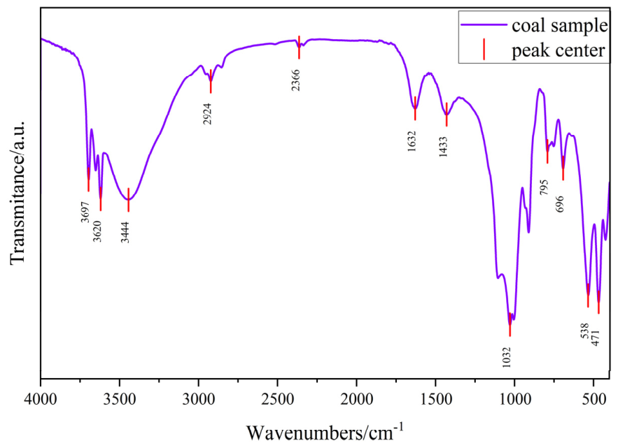
Figure 2.
XRD phase analysis diagram.
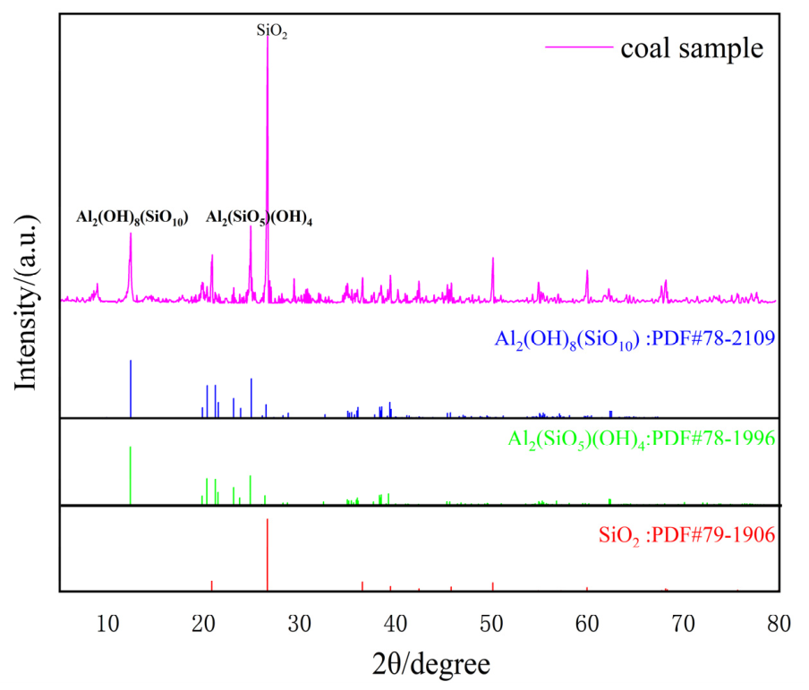
Figure 3.
Particle size distribution.
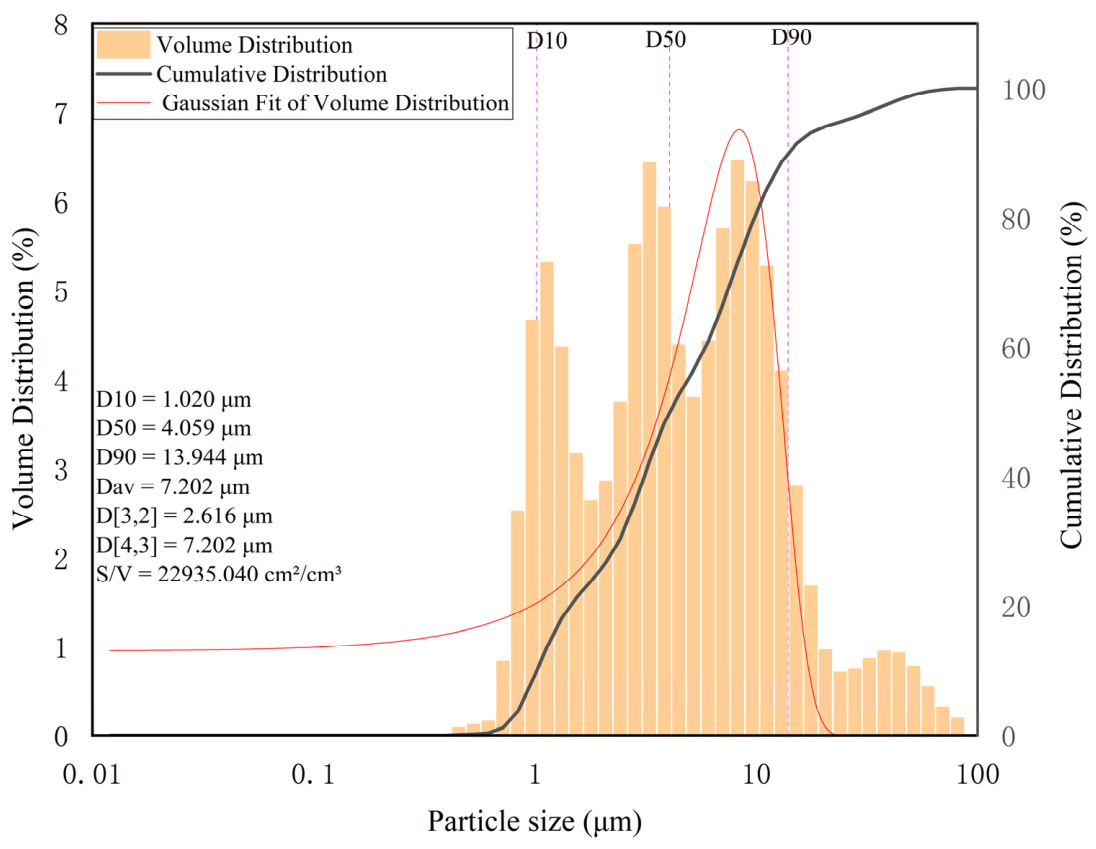
Figure 4.
Turbidity response surface: coal slurry concentration × PAM concentration.
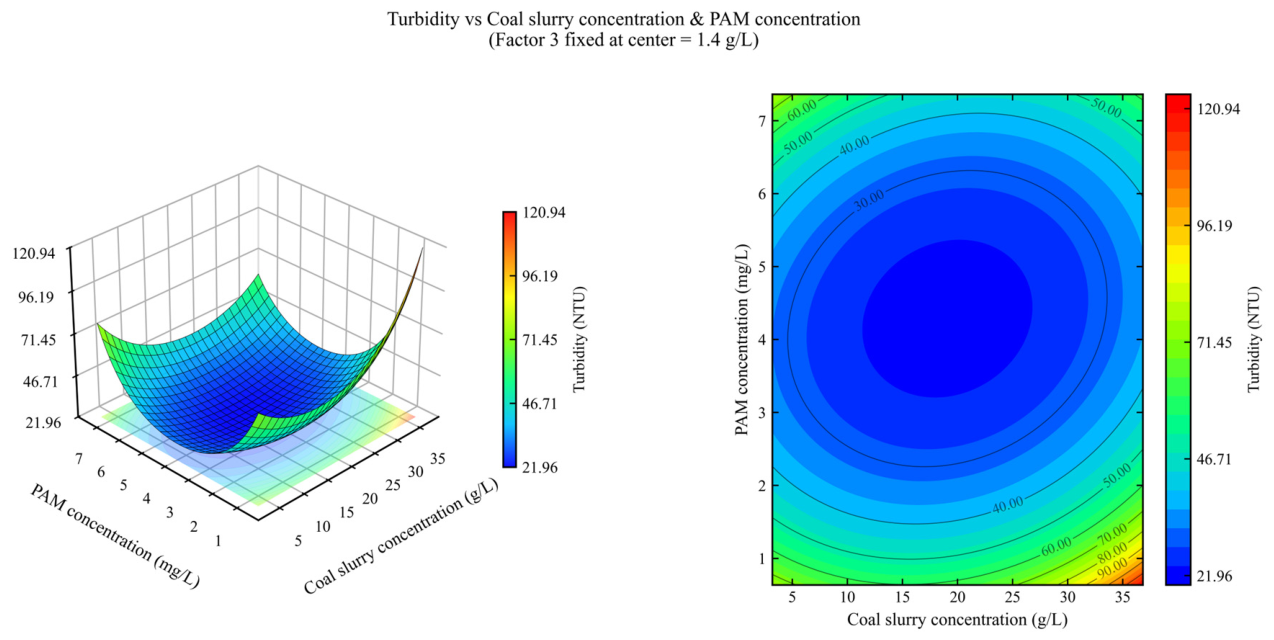
Figure 5.
Turbidity response surface: coal slurry concentration × CaCl2 concentration.
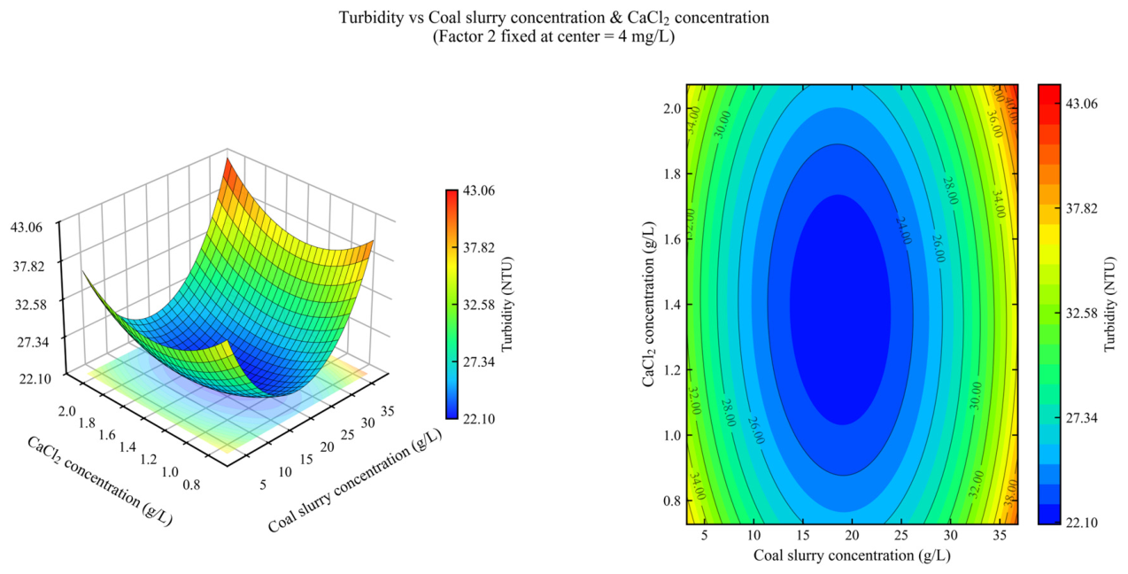
Figure 6.
Turbidity response surface: PAM concentration × CaCl2 concentration.
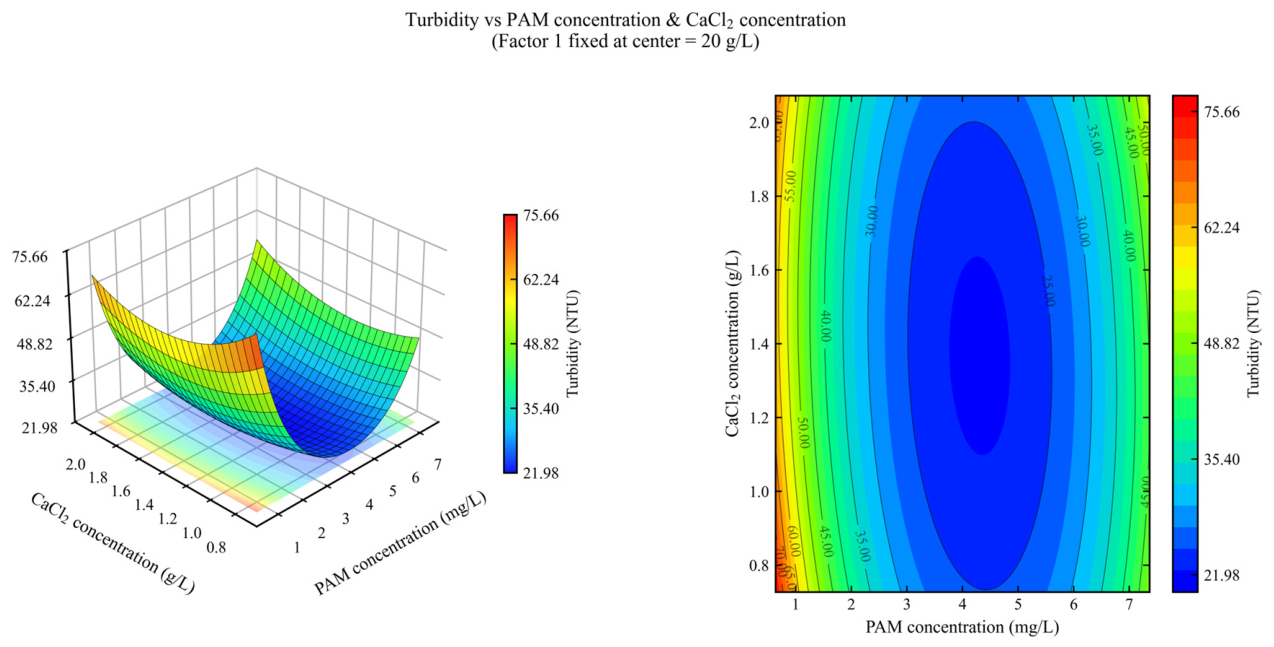
Figure 7.
Settling velocity response surface: coal slurry concentration × PAM concentration.
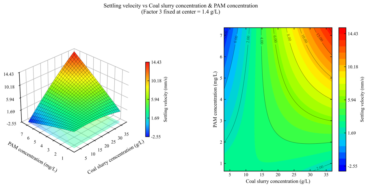
Figure 8.
Settling velocity response surface: coal slurry concentration × CaCl2 concentration.
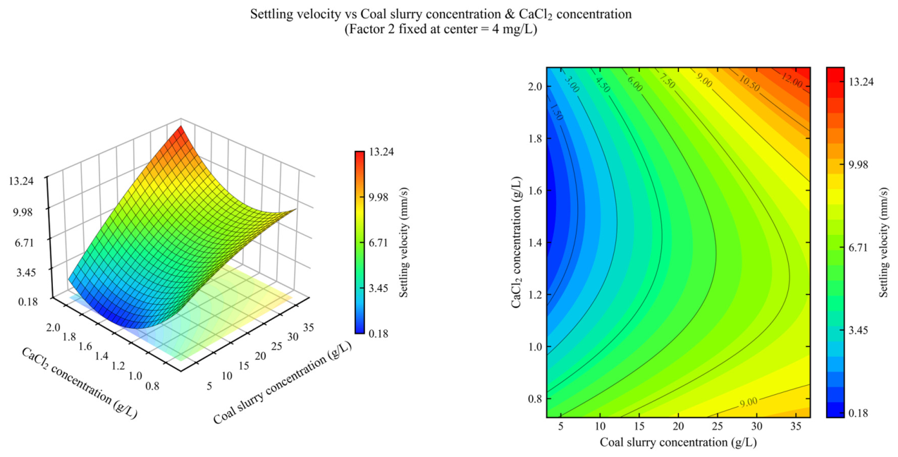
Figure 9.
Settling velocity response surface: PAM concentration × CaCl2 concentration.
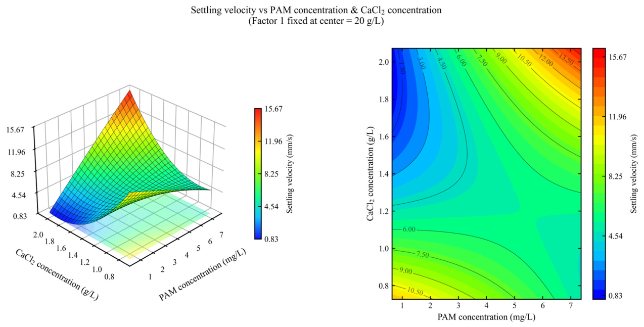
Figure 10.
HuberT robust regression diagnostic plots for the turbidity ln(Y1) model: (a)measured versus predicted values; (b) residuals versus predicted values; (c) robust weight distribution.
Figure 10.
HuberT robust regression diagnostic plots for the turbidity ln(Y1) model: (a)measured versus predicted values; (b) residuals versus predicted values; (c) robust weight distribution.
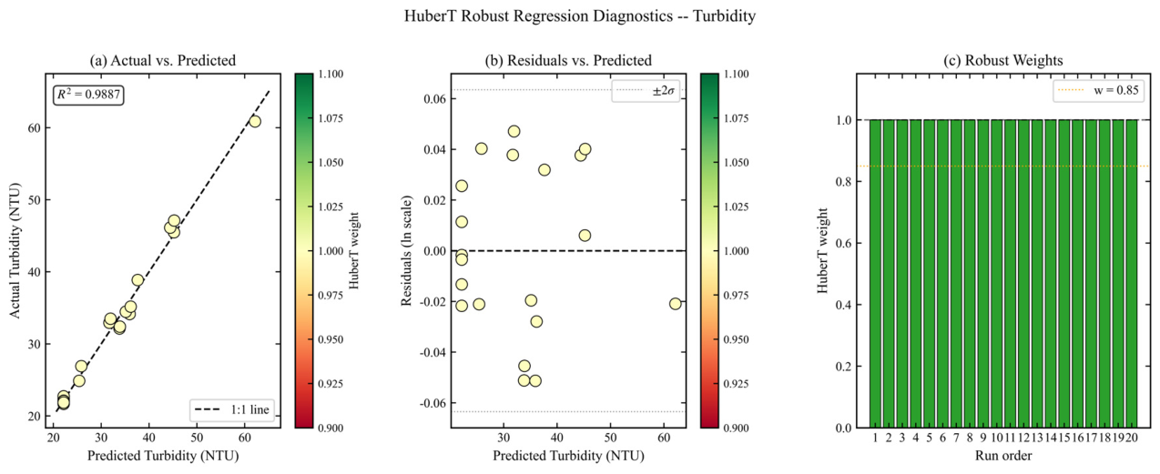
Figure 11.
HuberT robust regression diagnostic plots for the settling velocity Y2 model: (a) measured versus predicted values; (b) residuals versus predicted values; (c) robust weight distribution.
Figure 11.
HuberT robust regression diagnostic plots for the settling velocity Y2 model: (a) measured versus predicted values; (b) residuals versus predicted values; (c) robust weight distribution.
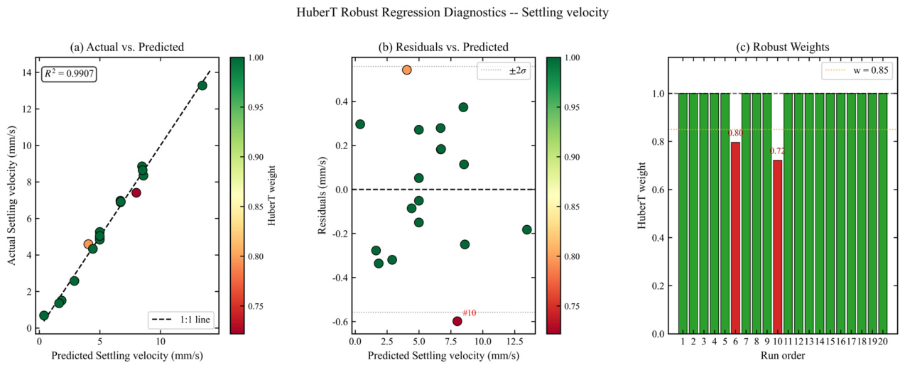

Table 1.
Calorific value and ash content.
| Bomb calorific value Qb,ad | Air-dried basis gross calorific value Qgr,V,ad | Dry basis gross calorific value Qgr,V,d | Air-dried basis net calorific value Qnet,V,ad | Ash content |
| J/g | % | |||
| 16276 | 16246 | 16409 | 15708 | 39.00 |
Table 2.
Positions and assignments of the major FTIR absorption peaks.
| Wavenumber (cm−1) | Transmittance (%) | Prominence | Peak shape | Assignment |
| 3697 | 54.62 | 15.68 | Sharp | —OH stretching vibration, kaolinite inner-surface hydroxyl |
| 3620 | 48.34 | 14.87 | Sharp | —OH stretching vibration, kaolinite inner hydroxyl |
| 3444 | 48.08 | 51.61 | Broad | O—H stretching vibration of adsorbed/interlayer water (hydrogen-bonded) |
| 2924 | 86.21 | 4.96 | Weak | Aliphatic —CH2—/—CH3 stretching vibration |
| 2366 | 97.16 | 2.19 | Very weak | Atmospheric CO2 background interference |
| 1632 | 77.34 | 11.47 | Medium | Aromatic C=C skeletal vibration + H2O bending vibration |
| 1433 | 75.41 | 5.52 | Weak | —CH2—/—CH3 bending vibration |
| 1032 | 7.53 | 76.12 | Strong (strongest peak) | Si—O—Si asymmetric stretching vibration |
| 795 | 63.47 | 10.12 | Medium | Si—O—Al vibration |
| 696 | 58.11 | 11.18 | Medium | Si—O bending vibration |
| 538 | 17.06 | 23.02 | Strong | Si—O—Al bending vibration |
| 471 | 14.82 | 38.89 | Strong | Si—O—Si bending vibration |
Note: ᵃ The peak at 2366 cm−1 is attributed to atmospheric CO2 background interference and was not included in the mineral phase assignment.
Table 3.
Volume percentage distribution across particle size intervals.
| Size interval | Volume percentage (%) | Description |
| <1 μm | 8.36 | Ultrafine particles (mainly clay mineral microparticles) |
| 1–5 μm | 44.30 | Dominant size interval, largest fraction |
| 5–10 μm | 26.59 | Secondary dominant interval |
| 10–20 μm | 13.82 | Coarser particle interval |
| 20–50 μm | 5.13 | Coarse particle interval |
| 50–100 μm | 1.81 | Very coarse particles/aggregates, very small fraction |
Table 4.
Particle size characteristic parameters.
| Parameter | Value | Description |
| D10 | 1.020 μm | Particle size below which 10% of particles fall |
| D50 | 4.059 μm | Median particle size |
| D90 | 13.944 μm | Particle size below which 90% of particles fall |
| Dav | 7.202 μm | Volume-weighted mean diameter |
| D [3,2] | 2.616 μm | Surface area-weighted mean diameter (Sauter diameter) |
| D [4,3] | 7.202 μm | Volume-weighted mean diameter |
| S/V | 22935.040 cm2/cm3 | Specific surface area (volume basis) |
| Span | 3.18 | Distribution width = (D90−D10)/D50 |
Table 5.
Factor levels of the central composite design.
| Factor | Symbol | −1.682 | −1 | 0 | +1 | +1.682 |
| Coal slurry mass concentration (g/L) | A | 3.18 | 10 | 20 | 30 | 36.82 |
| PAM mass concentration (mg/L) | B | 0.64 | 2 | 4 | 6 | 7.36 |
| CaCl2 mass concentration (g/L) | C | 0.73 | 1 | 1.4 | 1.8 | 2.07 |
Table 6.
Central composite design matrix and measured response values.
| Run | A (g/L) | B (mg/L) | C (g/L) | Y1 Turbidity (NTU) | Y2 Settling velocity (mm/s) |
| 1 | 10.00 | 2.00 | 1.00 | 38.86 | 6.971 |
| 2 | 30.00 | 2.00 | 1.00 | 45.487 | 6.888 |
| 3 | 10.00 | 6.00 | 1.00 | 32.14 | 1.506 |
| 4 | 30.00 | 6.00 | 1.00 | 32.93 | 8.852 |
| 5 | 10.00 | 2.00 | 1.80 | 34.15 | 1.356 |
| 6 | 30.00 | 2.00 | 1.80 | 46.13 | 4.593 |
| 7 | 10.00 | 6.00 | 1.80 | 34.458 | 4.3345 |
| 8 | 30.00 | 6.00 | 1.80 | 32.39 | 13.278 |
| 9 | 3.18 | 4.00 | 1.40 | 33.492 | 0.688 |
| 10 | 36.82 | 4.00 | 1.40 | 35.17 | 7.406 |
| 11 | 20.00 | 0.64 | 1.40 | 60.873 | 2.577 |
| 12 | 20.00 | 7.36 | 1.40 | 47.113 | 6.914 |
| 13 | 20.00 | 4.00 | 0.73 | 24.87 | 8.345 |
| 14 | 20.00 | 4.00 | 2.07 | 26.91 | 8.643 |
| 15 | 20.00 | 4.00 | 1.40 | 22.40 | 5.042 |
| 16 | 20.00 | 4.00 | 1.40 | 22.72 | 5.261 |
| 17 | 20.00 | 4.00 | 1.40 | 22.11 | 4.939 |
| 18 | 20.00 | 4.00 | 1.40 | 21.67 | 4.840 |
| 19 | 20.00 | 4.00 | 1.40 | 22.07 | 4.840 |
| 20 | 20.00 | 4.00 | 1.40 | 21.86 | 5.042 |
Table 7.
Analysis of variance (ANOVA) for the turbidity ln(Y1) model.
| Source | Sum of Squares | df | Mean Square | F-value | p-value | Significance |
| Model | 1.762663 | 9 | 0.195851 | 97.14 | < 0.0001 | Highly significant |
| A | 0.018536 | 1 | 0.018536 | 9.19 | 0.0126 | Significant |
| B | 0.121532 | 1 | 0.121532 | 60.28 | < 0.0001 | Highly significant |
| C | 0.000362 | 1 | 0.000362 | 0.18 | 0.6806 | Not significant |
| AB | 0.030700 | 1 | 0.030700 | 15.23 | 0.0030 | Highly significant |
| AC | 0.000407 | 1 | 0.000407 | 0.20 | 0.6628 | Not significant |
| BC | 0.003547 | 1 | 0.003547 | 1.76 | 0.2142 | Not significant |
| A2 | 0.330541 | 1 | 0.330541 | 163.95 | < 0.0001 | Highly significant |
| B2 | 1.373777 | 1 | 1.373777 | 681.40 | < 0.0001 | Highly significant |
| C2 | 0.038205 | 1 | 0.038205 | 18.95 | 0.0014 | Highly significant |
| Residual | 0.020161 | 10 | 0.002016 | |||
| Lack of Fit | 0.018715 | 5 | 0.003743 | 12.94 | 0.0069 | Highly significant |
| Pure Error | 0.001446 | 5 | 0.000289 | |||
| Cor Total | 1.782824 | 19 | ||||
| R2 = 0.9887, Adj-R2 = 0.9785, Pred-R2 = 0.9133, Adequate Precision = 32.50, CV = 1.30% | ||||||
Note: P ≤ 0.01 indicates a highly significant nonlinear relationship; P ≤ 0.05 indicates a significant linear relationship; P > 0.05 indicates a non-significant linear relationship.
Table 8.
Analysis of variance (ANOVA) for the settling velocity Y2 model.
| Source | Sum of Squares | df | Mean Square | F-value | p-value | Significance |
| Model | 166.2928 | 9 | 18.4770 | 119.94 | < 0.0001 | Highly significant |
| A | 69.2036 | 1 | 69.2036 | 449.24 | < 0.0001 | Highly significant |
| B | 17.4939 | 1 | 17.4939 | 113.56 | < 0.0001 | Highly significant |
| C | 0.0018 | 1 | 0.0018 | 0.01 | 0.9168 | Not significant |
| AB | 21.5659 | 1 | 21.5659 | 140.00 | < 0.0001 | Highly significant |
| AC | 3.0239 | 1 | 3.0239 | 19.63 | 0.0013 | Highly significant |
| BC | 28.7477 | 1 | 28.7477 | 186.62 | < 0.0001 | Highly significant |
| A2 | 1.2995 | 1 | 1.2995 | 8.44 | 0.0157 | Significant |
| B2 | 0.0408 | 1 | 0.0408 | 0.27 | 0.6178 | Not significant |
| C2 | 23.3157 | 1 | 23.3157 | 151.35 | < 0.0001 | Highly significant |
| Residual | 1.5405 | 10 | 0.1540 | |||
| Lack of Fit | 1.4142 | 5 | 0.2828 | 11.20 | 0.0095 | Highly significant |
| Pure Error | 0.1262 | 5 | 0.0252 | |||
| Cor Total | 167.8333 | 19 | ||||
| R2 = 0.9908, Adj-R2 = 0.9826, Pred-R2 = 0.9315, Adequate Precision = 47.12, CV = 6.99% | ||||||
Note: P ≤ 0.01 indicates a highly significant nonlinear relationship; P ≤ 0.05 indicates a significant linear relationship; P > 0.05 indicates a non-significant linear relationship.
Table 9.
Exact HuberT robust weights.
| Run | Measured turbidity (NTU) | ln(Y1) weight | Flag | Measured settling velocity (mm/s) | Y2 weight | Flag |
| 1 | 38.860 | 1.0000 | 6.971 | 1.0000 | ||
| 2 | 45.487 | 1.0000 | 6.888 | 1.0000 | ||
| 3 | 32.137 | 1.0000 | 1.506 | 1.0000 | ||
| 4 | 32.933 | 1.0000 | 8.852 | 1.0000 | ||
| 5 | 34.147 | 1.0000 | 1.356 | 1.0000 | ||
| 6 | 46.130 | 1.0000 | 4.593 | 0.7961 | * | |
| 7 | 34.458 | 1.0000 | 4.335 | 1.0000 | ||
| 8 | 32.393 | 1.0000 | 13.278 | 1.0000 | ||
| 9 | 33.492 | 1.0000 | 0.688 | 1.0000 | ||
| 10 | 35.170 | 1.0000 | 7.406 | 0.7221 | * | |
| 11 | 60.873 | 1.0000 | 2.577 | 1.0000 | ||
| 12 | 47.113 | 1.0000 | 6.914 | 1.0000 | ||
| 13 | 24.870 | 1.0000 | 8.345 | 1.0000 | ||
| 14 | 26.907 | 1.0000 | 8.643 | 1.0000 | ||
| 15 | 22.403 | 1.0000 | 5.042 | 1.0000 | ||
| 16 | 22.723 | 1.0000 | 5.261 | 1.0000 | ||
| 17 | 22.111 | 1.0000 | 4.939 | 1.0000 | ||
| 18 | 21.673 | 1.0000 | 4.840 | 1.0000 | ||
| 19 | 22.072 | 1.0000 | 4.840 | 1.0000 | ||
| 20 | 21.857 | 1.0000 | 5.042 | 1.0000 |
Note: * indicates a downweighted point.
Table 10.
Multi-response optimization results.
| Optimization objective | Coal slurry concentration (g/L) | PAM concentration (mg/L) | CaCl2 concentration (g/L) | Predicted turbidity (NTU) | Predicted settling velocity (mm/s) | D value |
| Overall optimum | 25.27 | 5.19 | 2.07 | 29.21 | 13.26 | 0.8981 |
| V1 | 19.15 | 4.31 | 1.37 | 21.96 | — | — |
| V2 | 36.82 | 7.36 | 2.07 | — | 25.07 | — |
Note: V1, single-objective optimum for minimum turbidity; V2, single-objective optimum for maximum settling velocity.
Table 11.
Canonical analysis results.
| Model | Stationary point coordinates (coded A, B, C) | Within design space? | Hessian eigenvalues | Nature of stationary point |
| ln(Y1) Turbidity | (−0.090, 0.146, −0.074) | Yes | 0.051, 0.146, 0.315 (all positive) | Minimum |
| Y2 Settling velocity | (−14.523, −10.387, 11.317) | No | −1.093, 0.050, 1.963 (one negative, two positive) | Saddle point |
Disclaimer/Publisher’s Note: The statements, opinions and data contained in all publications are solely those of the individual author(s) and contributor(s) and not of MDPI and/or the editor(s). MDPI and/or the editor(s) disclaim responsibility for any injury to people or property resulting from any ideas, methods, instructions or products referred to in the content. |
© 2026 by the authors. Licensee MDPI, Basel, Switzerland. This article is an open access article distributed under the terms and conditions of the Creative Commons Attribution (CC BY) license.
Copyright: This open access article is published under a Creative Commons CC BY 4.0 license, which permit the free download, distribution, and reuse, provided that the author and preprint are cited in any reuse.