

Submitted:
17 July 2026
Posted:
20 July 2026
You are already at the latest version
Abstract
Short-term particulate-matter forecasts are strongly influenced by temporal persistence, which can obscure the incremental value of meteorological covariates and seasonality. This study evaluates that incremental value using 42,823 hourly observations of PM10 and meteorological conditions from Kraków, Poland, collected during 2020–2024. Four interpretable Bayesian lognormal regression models were compared with historical-median, persistence, and rolling one-step-ahead SARIMAX references. The models progressively incorporated lagged PM10, standardized meteorological predictors, and annual and daily Fourier terms. Evaluation used four rolling-origin validation folds and an untouched final 20% test period. On the final test set, the full Bayesian model achieved MAE 4.865 μgm−3, RMSE 7.453 μgm−3, CRPS 3.602 μgm−3, and 0.884 coverage of its nominal 90% predictive interval. Its point accuracy was statistically indistinguishable from persistence, the lag-only Bayesian model, and SARIMAX under moving-block bootstrap. However, the full model had the best PSIS-LOO expected log predictive density and the lowest test-set CRPS. Meteorological effects were strongly attenuated after including lagged PM10, while persistence remained the best point predictor during high-pollution hours. The results show that temporal persistence dominates one-hour-ahead point prediction, whereas meteorology and cyclic seasonality provide more evident benefits for probabilistic distributional modeling than for MAE or RMSE.
Keywords:
PM10
; air pollution
; Bayesian regression
; probabilistic forecasting
; temporal persistence
; meteorological covariates
; PSIS-LOO
; rolling-origin validation
1. Introduction
A central difficulty in evaluating short-term models is that successive measurements are strongly dependent. A model containing the previous-hour concentration can appear markedly better than a meteorology-only regression even when the added meteorological variables contribute little beyond persistence. Consequently, a scientifically useful comparison should distinguish three questions: whether lagged dominates one-step-ahead forecasts, whether meteorology and seasonality add information beyond that lag, and whether any gain is visible in point errors, predictive distributions, or both. It should also compare the proposed model with a direct persistence forecast and with a conventional dynamic-regression benchmark under the same rolling one-step evaluation protocol.
This study addresses these questions using five years of hourly observations from Kraków. Four nested Bayesian models are considered: a lag-only model (M0), a meteorology-only model (M1), a meteorology-plus-seasonality model (M2), and a full model combining lagged , meteorology, and cyclic seasonality (M3). They are compared with a historical-median baseline, persistence, and SARIMAX. Chronological rolling-origin validation, an untouched final test period, probabilistic scores, PSIS-LOO, posterior predictive checks, and moving-block bootstrap comparisons are used to avoid relying on a single favorable metric.
The principal contributions are:
- an interpretable ablation design that separates the contribution of lagged , meteorological covariates, and cyclic annual and daily effects;
- a fair rolling one-step-ahead comparison with persistence and SARIMAX;
- joint assessment of point accuracy, predictive-distribution quality, interval calibration, and high-pollution performance;
- an analysis of how meteorological coefficient estimates change after short-term persistence is represented explicitly; and
- a fully reproducible Stan/Python workflow with explicit time-split, scaling, diagnostic, and sensitivity checks.
2. Materials and Methods
2.1. Data Sources and Study Period
The analysis used hourly observations from 1 January 2020 through 31 December 2024 at the Kraków Złoty Róg air-quality station (GIOŚ sensor ID 16786; station code MpKrakZloRog-PM10-1g; coordinates 50.081197∘ N, 19.895358∘ E). Air-quality measurements were obtained through the archival API of the Polish Chief Inspectorate of Environmental Protection (GIOŚ) [15]. Meteorological data were queried at the same coordinates from the Open-Meteo Historical Weather API [14]. The meteorological variables were temperature at 2 m, relative humidity at 2 m, wind speed at 10 m, and surface pressure.
Using the same coordinates for both sources avoided an additional spatial offset between the pollution monitor and the meteorological query point. Table 1 summarizes the study period, variables, and final split.
2.2. Data Preparation and Forecasting Information Set
Both sources were placed on a complete hourly grid and ordered chronologically. Missing values were not interpolated; rows without an observed target were excluded. Meteorological gaps could be forward-filled for at most two consecutive hours. Ten air-quality rows associated with five duplicated, DST-ambiguous timestamps were explicitly removed rather than silently deduplicated. The resulting modeling table contained 42,823 observations after lag construction.
The target was the one-hour-ahead concentration . Forecasts for hour t used only information available by hour : the observed where applicable, meteorological variables lagged by one hour, and deterministic calendar terms. Let
where each meteorological predictor was standardized using the mean and standard deviation of the corresponding training window only. The centered lag variable was
All scaling parameters were fitted separately within each cross-validation fold and once on the final 80% training period. No transformation parameter was estimated from validation or test observations.
Cyclic seasonality was represented by two annual and two daily Fourier harmonics. For period P and harmonic order ,
with hours for the annual component and hours for the daily component.
2.3. Bayesian Regression Models
For each Bayesian model,
where is the model-specific predictor on the log scale and is the residual scale.
The four Bayesian specifications were:
The persistence coefficient was constrained to by .
Table 2 summarizes all Bayesian and reference models.
The priors were
Prior predictive simulations were used to check that these distributions permitted a broad but plausible range of concentrations.
2.4. Reference Models
B0 predicted the training-period median for every evaluation hour. B1 was deterministic persistence, . B2 was a SARIMAX dynamic regression fitted to with an AR(1) component and the same lagged meteorological and Fourier regressors used by the Bayesian specifications, implemented with Statsmodels [27]. SARIMAX parameters were fitted once within each training window. Evaluation then proceeded one hour at a time: a one-step forecast was generated, the observed value was appended to the state without parameter refitting, and the next forecast was produced. This matched the information available to persistence and the lag-containing Bayesian models.
Figure 1 summarizes the nested Bayesian model sequence through directed dependency diagrams. The diagrams are explanatory graphical summaries of each model specification and are not intended as causal-identification assumptions.
2.5. Inference and Diagnostics
[21,22]. Four chains were run, each with 1000 warm-up and 1000 retained iterations, target acceptance probability 0.90, and maximum tree depth 12. Sampling quality was assessed using rank-normalized , bulk and tail effective sample sizes, divergent transitions, maximum-tree-depth hits, and E-BFMI. Posterior processing and PSIS-LOO calculations used ArviZ [23].
2.6. Chronological Validation and Predictive Metrics
The data were split chronologically. The first 80% formed the final training set and the last 20% an untouched held-out test set. Model development on the first 80% used four expanding-window rolling-origin folds. The initial training window covered the first 60% of all observations, and each validation window covered the next 5%; later folds incorporated earlier validation windows into training. Figure 2 shows the time series and all split boundaries.
Point forecasts were evaluated using MAE and RMSE. Probabilistic forecasts were evaluated using the continuous ranked probability score (CRPS), empirical coverage of the 50% and 90% predictive intervals, and mean interval width. CRPS is a proper scoring rule that rewards both calibration and concentration of a predictive distribution [25]. The deterministic B0 and B1 forecasts were additionally treated as degenerate distributions when reporting CRPS; they do not provide genuine interval forecasts.
For Bayesian models, PSIS-LOO and WAIC were calculated as complementary measures of full predictive-density fit [24]. Because ordinary pointwise LOO does not reproduce a future-block forecasting task, chronological cross-validation and the final held-out test remained the primary evidence for out-of-time performance.
Pairwise uncertainty in metric differences was assessed using a paired moving-block bootstrap [26]. Two thousand resamples were generated with a primary block length of 24 hours and a sensitivity block length of 168 hours. High-pollution performance was assessed for test observations above the 90th percentile of the training-period distribution (58.7 ).
3. Results
3.1. Data Characteristics and Prior Predictive Assessment
The final modeling dataset contained 42,823 hourly observations. The final training set contained 34,258 observations, and the held-out test set contained 8565 observations from 31 December 2023 19:00 through 31 December 2024 23:00. The observed series displayed pronounced right skewness, seasonal variation, and episodic peaks, including concentrations above 200 in several winter periods (Figure 2).
Detailed prior predictive checks are provided in Supplementary Figure S1.
3.2. Sampling Diagnostics
All final Bayesian fits satisfied the diagnostic criteria. Maximum was 1.000 for M0–M3, minimum bulk ESS exceeded 2000, minimum tail ESS exceeded 2200, and no divergent transitions or maximum-tree-depth hits occurred. Minimum E-BFMI ranged from 0.868 to 1.008. Full values are reported in Supplementary Table S1.
3.3. Overall Predictive Performance
Table 3 and Figure 3 summarize final test-set performance. The historical-median baseline was clearly inadequate (MAE 13.013 ). Models without lagged also performed poorly: M1 and M2 had MAE values of 11.605 and 11.374 , respectively. Adding cyclic seasonality to meteorology alone yielded only a modest improvement.
The four persistence-aware models were tightly grouped. M3 achieved the lowest MAE (4.865 ) and CRPS (3.602 ). Persistence had MAE 4.886 , SARIMAX had MAE 4.884 and CRPS 3.622 , and M0 had MAE 4.930 and CRPS 3.659 . The lowest RMSE was obtained by persistence (7.320 ), closely followed by M0 (7.332), SARIMAX (7.426), and M3 (7.453). Thus, the ranking differed slightly between absolute-error, squared-error, and distributional criteria.
The probabilistic intervals were reasonably calibrated. Coverage of nominal 90% intervals was 0.885 for SARIMAX, 0.889 for M0, 0.873 for M1, 0.872 for M2, and 0.884 for M3. M3 produced the narrowest 90% interval among the probabilistic persistence-aware models (22.957 ), marginally narrower than SARIMAX and M0.
The rolling-origin validation folds showed the same qualitative pattern: M3 had the best mean MAE, RMSE, and CRPS among the probabilistic models, followed closely by SARIMAX and M0, while M1 and M2 were substantially worse. This agreement reduces the likelihood that the final ranking resulted solely from a favorable final-year realization.
3.4. Uncertainty in Differences Between Models
The point differences among M3, persistence, M0, and SARIMAX were small relative to temporally dependent variation in forecast errors. Table 4 reports paired moving-block bootstrap comparisons for the 24-hour blocks. None of the 95% intervals for MAE or RMSE differences excluded zero. For example, the observed M3-minus-persistence MAE difference was , with a 95% interval of .
For CRPS, the evidence favored M3 more consistently but remained slightly below a strict 95% threshold on the single held-out year. Relative to M0, the observed CRPS difference was , with and a 95% interval of . Relative to SARIMAX, the difference was , with and interval . The 168-hour block-length sensitivity analysis led to the same substantive conclusion.
3.5. Predictive Density and Posterior Predictive Behavior
PSIS-LOO and WAIC provided a clearer separation of the predictive distributions than the final-year point metrics. M3 had the highest expected log pointwise predictive density, exceeding M0 by 1321.8 elpd units with a standard error of the difference of 52.1. M1 and M2 were more than 24,000 elpd units behind M3. Figure 4 shows the PSIS-LOO ranking relative to M3 together with the associated Pareto-k diagnostics. All maximum Pareto-k values were below 0.24, indicating stable PSIS approximations. Full numerical results are provided in Supplementary Table S2.
Posterior predictive checks also favored M3. The observed training-data 99th percentile was 100.6 ; the median replicated value was 99.9 for M3, compared with 102.2 for M0, 108.7 for M1, and 111.3 for M2. The lag-containing models also left substantially less short-lag autocorrelation in test residuals than the meteorology-only models (Supplementary Figure S2).
Figure 5 illustrates M3 and persistence during a representative winter test interval. The predictive median tracked the evolution of the episode closely, while the predictive interval widened during the sharp increase. The largest observed peak, 227 , remained difficult to anticipate precisely, reflecting the challenge of sudden extreme episodes.
3.6. Meteorological Effects and Temporal Persistence
The contrast between M1 and M3 was substantial (Table 5, Figure 6). In M1, a one-standard-deviation increase in lagged temperature was associated with a 22.6% decrease in median , and wind speed with a 23.4% decrease. After lagged was included, these effects shrank to 2.0% and 4.2%, respectively. The humidity effect shrank from % to %, and the surface-pressure effect from % to %.
The autoregressive coefficient was 0.914 (90% interval 0.910–0.917) in M0 and 0.865 (0.860–0.869) in M3. The lower M3 coefficient is consistent with meteorology and cyclic terms explaining a portion of variation that otherwise appears as pure persistence, although the lag term remains dominant.
3.7. Performance During High-Pollution Hours
The high-pollution subset contained 636 test hours above 58.7 . All models had larger errors in this regime, but the relative ranking changed. Persistence was the best point predictor, with MAE 10.4 and RMSE 14.6 . M0, M3, and SARIMAX had MAE values of 12.8, 13.0, and 13.2 , respectively (Figure 7). The meteorology-only models deteriorated much more strongly, with MAE above 41 . Therefore, M3’s overall distributional advantage should not be interpreted as uniformly superior point prediction during extreme episodes.
3.8. Sensitivity Analysis
Widening the meteorological coefficient prior from to had negligible effects on predictions and coefficient intervals. Replacing the lognormal model with a Student-t likelihood on log- reduced MAE and CRPS slightly but increased RMSE by 28.5%, indicating greater tolerance of typical errors at the cost of occasional large misses. These results did not overturn the main ranking but show that tail-sensitive conclusions depend on the likelihood family (Supplementary Figure S4 and Tables S3–S4).
4. Discussion
4.1. Temporal Persistence as the Dominant Short-Horizon Signal
The primary empirical result is that one-hour-ahead point forecasting is dominated by the most recent observation. M1 and M2, which excluded the lag term, were markedly inferior to persistence-aware models. By contrast, M3, M0, persistence, and SARIMAX differed by only hundredths of a in MAE. The block bootstrap showed that these point-error differences were not distinguishable from zero at the 95% level.
In the present analysis, however, the explicit M0 and persistence comparisons show that this improvement should not be attributed automatically to the meteorological part of a dynamic model. Much of the attainable one-hour point accuracy is already captured by persistence.
The distinction is important methodologically. Comparing M3 only with M1 or M2 would suggest a dramatic improvement from the full Bayesian specification. Comparing it with persistence and M0 reveals a more modest incremental contribution. This illustrates why a direct persistence baseline and matched rolling one-step protocol are essential in short-horizon environmental forecasting.
4.2. Where Meteorology and Seasonality Add Value
Meteorology and cyclic seasonality provided limited incremental value in MAE and RMSE but more visible value in the full predictive distribution. M3 achieved the lowest test CRPS, the highest PSIS-LOO elpd, good interval calibration, and the closest posterior reproduction of the observed upper-tail quantile. These gains are meaningful for applications that require exceedance probabilities or uncertainty intervals rather than only a single central prediction.
The bootstrap evidence for CRPS was directionally strong but not conclusive under a strict 95% criterion: was approximately 0.94 against M0 and 0.92 against SARIMAX. PSIS-LOO produced a much clearer separation because it aggregated full log predictive densities across the training observations. Nevertheless, the chronological test and rolling-origin results remain the more direct evidence for future-time forecasting; LOO should be interpreted as complementary evidence about predictive-density fit rather than a replacement for time-respecting validation.
4.3. Interpretation of Meteorological Associations
The magnitude of these associations depended strongly on whether temporal persistence was included. The apparent M1 temperature and wind effects were reduced by approximately an order of magnitude in M3. This attenuation indicates that meteorological variables in a static model partly proxy for persistent pollution episodes and their seasonal context. The M3 effects remain conditional associations, not causal effects: unmodeled emissions, boundary-layer dynamics, traffic, and heating demand can influence both meteorology and pollution.
Replacing four categorical seasons from the first manuscript version with cyclic Fourier terms also avoided artificial discontinuities at season boundaries and represented both daily and annual periodicity.
4.4. High-Pollution Episodes
The high-pollution analysis changes the practical interpretation. Persistence was the best point predictor above the training 90th percentile, while M3 had higher MAE and RMSE in that subset. Sudden peaks are difficult for smooth probabilistic regressions because the preceding hour may be more informative than meteorological variables that change gradually. This does not negate M3’s overall calibration and distributional performance, but it shows that an operational alert system should not assume uniform improvement across regimes.
Future operational extensions could model exceedance events or regime changes directly, incorporate emission-related variables, or combine calibrated probabilistic forecasts with a persistence-based safeguard during rapidly developing episodes. Such developments would constitute new experiments and are outside the scope of the present study.
4.5. Strengths and Limitations
The nested M0–M3 design further separates the contributions of persistence, meteorology, and seasonality, and the validation framework prevents the final test year from influencing preprocessing or model selection.
The study also has limitations. First, all observations come from a single Kraków station, so the estimates may reflect local emission sources, urban structure, topography, and sensor context. The results cannot be assumed to generalize directly to other cities or monitoring stations without recalibration. Second, the meteorological predictors were obtained from a gridded historical-weather service rather than a co-located physical weather station. Third, traffic, residential heating, industrial activity, boundary-layer height, precipitation, and gaseous co-pollutants were not included. Fourth, the moving-block bootstrap used one held-out year; it accounts for serial dependence within that year but does not provide multiple independent annual test replications. Finally, the Student-t sensitivity result indicates that tail-related conclusions depend partly on the likelihood specification.
5. Conclusions
The corrected five-year analysis shows that lagged is the dominant source of one-hour-ahead point accuracy. Models without the lag term were substantially worse, whereas M3, M0, persistence, and SARIMAX had statistically indistinguishable MAE and RMSE on the final test year.
The full M3 specification nevertheless provided the strongest overall probabilistic evidence: it had the lowest test CRPS, the best PSIS-LOO elpd, calibrated 90% intervals, and posterior predictive upper-tail behavior closest to the observed data. Meteorological effects became much smaller after lagged was introduced, demonstrating that static meteorology-only regressions can overstate associations by absorbing short-term persistence.
At the same time, persistence remained the best point predictor during high-pollution hours, so the full model should not be presented as uniformly superior across all regimes.
The main practical conclusion is therefore nuanced: for one-hour-ahead forecasts, meteorology and cyclic seasonality add little to central point accuracy beyond the most recent concentration, but they add clearer value to the quality and interpretation of the predictive distribution. External validation at additional stations and explicit modeling of high-pollution regimes are the most relevant directions for future work.
Supplementary Materials
The following supporting information can be downloaded at the website of this paper posted on Preprints.org: Figure S1: Prior predictive checks; Figure S2: Residual diagnostics; Figure S3: PSIS-LOO comparison and Pareto-k diagnostics; Figure S4: Sensitivity of M3 to prior width and likelihood family; Table S1: MCMC diagnostics; Table S2: PSIS-LOO and WAIC comparison; Table S3: Sensitivity metrics; Table S4: Sensitivity materiality assessment. A compiled supplementary file is included in this package as supplementary_material.pdf.
Author Contributions
Conceptualization, S.P. and J.B.; methodology, S.P. and J.B.; software, S.P.; validation, S.P. and J.B.; formal analysis, S.P.; investigation, S.P.; data curation, S.P.; writing—original draft preparation, S.P.; writing—review and editing, S.P. and J.B.; visualization, S.P.; supervision, J.B.; project administration, J.B.; funding acquisition, J.B. All authors have read and agreed to the published version of the manuscript.
Funding
This research received no external funding.
Data Availability Statement
The air-quality observations are available from the Chief Inspectorate of Environmental Protection in Poland, and the meteorological variables are available through the Open-Meteo Historical Weather API. The analysis code, processed data, configurations, and scripts reproducing the reported tables and figures will be archived at [persistent repository URL/DOI to be inserted after acceptance].
Acknowledgments
During preparation of this manuscript, the authors used OpenAI ChatGPT 5.5 for language editing, restructuring, and assistance in integrating author-verified computational results into the manuscript. Authors also used Anthropic Claude Code Sonnet 4.6 and OpenAI Codex for code refactoring. The authors reviewed and edited all output and take full responsibility for the content of the publication.
Conflicts of Interest
The authors declare no conflicts of interest.
Abbreviations
The following abbreviations are used in this manuscript:
| ACF | Autocorrelation function |
| CRPS | Continuous ranked probability score |
| E-BFMI | Energy Bayesian fraction of missing information |
| ESS | Effective sample size |
| HMC | Hamiltonian Monte Carlo |
| MAE | Mean absolute error |
| MCMC | Markov chain Monte Carlo |
| PSIS-LOO | Pareto-smoothed importance-sampling leave-one-out cross-validation |
| RMSE | Root mean squared error |
| SARIMAX | Seasonal autoregressive integrated moving-average model with exogenous variables |
| WAIC | Widely applicable information criterion |
References
- Taheri Shahraiyni, Hamid; Sodoudi, Sahar. Statistical Modeling Approaches for PM10 Prediction in Urban Areas: A Review of 21st-Century Studies. Atmosphere 2016, 7(2), 15. [Google Scholar] [CrossRef]
- Bai, Lu; Wang, Jianzhou; Ma, Xuejiao; Lu, Haiyan. Air Pollution Forecasts: An Overview. Int. J. Environ. Res. Public Health 2018, 15(4), 780. [Google Scholar] [CrossRef] [PubMed]
- Kochanski, Adam K.; Beezley, Jonathan D.; Mandel, Jan; Clements, Craig B. Air Pollution Forecasting by Coupled Atmosphere-Fire Model WRF and SFIRE with WRF-Chem. arXiv. 2013. Available online: https://arxiv.org/abs/1304.7703.
- Wang, Shuo; Cheng, Yun; Meng, Qingye; Saukh, Olga; Zhang, Jiang; Fan, Jingfang; Zhang, Yuanting; Yuan, Xingyuan; Thiele, Lothar. PCDCNet: A Surrogate Model for Air Quality Forecasting with Physical-Chemical Dynamics and Constraints. arXiv. 2025. Available online: https://arxiv.org/abs/2505.19842.
- Abdullah, Siti; Napi, Nur Nazmi Liyana Mohd; Ahmed, Ali Najah; Mansor, Wan Nur Wani; Mansor, Ahmad Azam; Ismail, Mohd; Abdullah, Ahmad Makmom; Ramly, Zairith Zulaikha Tuan. Development of Multiple Linear Regression for Particulate Matter (PM10) Forecasting during Episodic Transboundary Haze Event in Malaysia. Atmosphere 2020, 11(3), 289. [Google Scholar] [CrossRef]
- Hosamane, S. N.; Prashanth, K. S.; Virupakshi, A. S. Assessment and Prediction of PM10 Concentration Using ARIMA. J. Phys. Conf. Ser. 2021, 1706, 012132. [Google Scholar] [CrossRef]
- Cusano, Marco; Gaeta, Andrea; Morelli, Roberto; Cattani, Giorgio; Canepari, Silvia; Massimi, Luca; Leone, Gianluca. Spatial Modeling of Trace Element Concentrations in PM10 Using Generalized Additive Models (GAMs). Atmosphere 2025, 16(4), 464. [Google Scholar] [CrossRef]
- Zarate Valencia, A. R.; Rodriguez Rosales, A. A. Application of Random Forest in a Predictive Model of PM10 Particles in Mexico City. Nat. Environ. Pollut. Technol. 2024, 23(2), 711–724. [Google Scholar] [CrossRef]
- Benedict, B. Anna; Vivek, C.; Priyadharshini, D.; Rihana, R.; Thirumalini, J.; Ali, Sameeha Anvar. Predicting PM2.5 and PM10 Using Machine Learning Models like Random Forest, Support Vector Machines and Artificial Neural Networks. TIJER Int. Res. J. 2025, 12(5), 1020–1029. [Google Scholar]
- Chaudhary, V.; Deshbhratar, A.; Kumar, V.; Paul, D. Time Series Based LSTM Model to Predict Air Pollutant’s Concentration for Prominent Cities in India. In Proceedings of the Utility and Data Mining Workshop, 2018. [Google Scholar]
- Karmoude, M.; Munhungewarwa, B.; Chiraira, I.; McKenzie, R.; Kong, J.; Smith, B.; Ayana, G.; Njara, N.; Mathaha, T.; Kumar, M.; Mellado, B. Machine Learning for Air Quality Prediction and Data Analysis: Review on Recent Advancements, Challenges, and Outlooks. Sci. Total Environ. 2025, 1002, 180593. [Google Scholar] [CrossRef] [PubMed]
- Fioravanti, Giulia; Martino, Sara; Cameletti, Michela; Cattani, Giorgio. Spatio-Temporal Modelling of PM10 Daily Concentrations in Italy Using the SPDE Approach. Atmos. Environ. 2021, 248, 118192. [Google Scholar] [CrossRef]
- Wang, K.; Ling, C.; Chen, Y.; Zhang, Z. Spatio-Temporal Joint Modelling on Moderate and Extreme Air Pollution in Spain. arXiv. 2023. Available online: https://arxiv.org/abs/2302.06059.
- Open-Meteo. Historical Weather API. 2026. Available online: https://open-meteo.com/en/docs/historical-weather-api. (accessed on 3 July 2026).
- Chief Inspectorate of Environmental Protection. Air Quality Data API in Poland. 2026. Available online: https://powietrze.gios.gov.pl/pjp/content/api. (accessed on 3 July 2026).
- Ramli, N.; Abdul Hamid, H.; Yahaya, A. S.; Ul-Saufie, A. Z.; Mohamed Noor, N.; Abu Seman, N. A.; Kamarudzaman, A. N.; Deak, G. Performance of Bayesian Model Averaging for Short-Term Prediction of PM10 Concentration in Peninsular Malaysia. Atmosphere 2023, 14(2), 311. [Google Scholar] [CrossRef]
- Zhalehdoost, A.; Taleai, M. Unravelling the Importance of Spatial and Temporal Resolutions in Modeling Urban Air Pollution Using a Machine Learning Approach. Sci. Rep. 2025, 15, 1–20. [Google Scholar] [CrossRef] [PubMed]
- Kliengchuay, W.; Worakhunpiset, S.; Limpanont, Y.; Meeyai, A. C.; Tantrakarnapa, K. Influence of Meteorological Conditions and Some Pollutants on PM10 Concentrations in Lamphun, Thailand. J. Environ. Health Sci. Eng. 2021, 19, 27–39. [Google Scholar] [CrossRef] [PubMed]
- Nistor, A.; Nistor, B.; Mihaila, D.; Bistricean, P.-I. Atmospheric Levels of PM10 in Relation to Meteorological Elements: Case Study of the Moldova Region, Romania. GEOREVIEW 2023, 33(1), 95–117. [Google Scholar] [CrossRef]
- Islam, N.; Toha, T. R.; Islam, M. M.; Ahmed, T. Spatio-Temporal Variation of Meteorological Influence on PM2.5 and PM10 over Major Urban Cities of Bangladesh. Aerosol Air Qual. Res. 2023, 23(1), 220082. [Google Scholar] [CrossRef]
- Carpenter, Bob; Gelman, Andrew; Hoffman, Matthew D.; Lee, Daniel; Goodrich, Ben; Betancourt, Michael; Brubaker, Marcus A.; Guo, Jiqiang; Li, Peter; Riddell, Allen. Stan: A Probabilistic Programming Language. J. Stat. Softw. 2017, 76(1), 1–32. [Google Scholar] [CrossRef] [PubMed]
- Hoffman, Matthew D.; Gelman, Andrew. The No-U-Turn Sampler: Adaptively Setting Path Lengths in Hamiltonian Monte Carlo. J. Mach. Learn. Res. 2014, 15, 1593–1623. [Google Scholar]
- Kumar, Ravin; Carroll, Colin; Hartikainen, Ari; Martin, Osvaldo. ArviZ: A Unified Library for Exploratory Analysis of Bayesian Models in Python. J. Open Source Softw. 2019, 4(33), 1143. [Google Scholar] [CrossRef]
- Vehtari, Aki; Gelman, Andrew; Gabry, Jonah. Practical Bayesian Model Evaluation Using Leave-One-Out Cross-Validation and WAIC. Stat. Comput. 2017, 27, 1413–1432. [Google Scholar] [CrossRef]
- Gneiting, Tilmann; Raftery, Adrian E. Strictly Proper Scoring Rules, Prediction, and Estimation. J. Am. Stat. Assoc. 2007, 102(477), 359–378. [Google Scholar] [CrossRef]
- Kunsch, Hans R. The Jackknife and the Bootstrap for General Stationary Observations. Ann. Stat. 1989, 17(3), 1217–1241. [Google Scholar] [CrossRef]
- Seabold, Skipper; Perktold, Josef. Statsmodels: Econometric and Statistical Modeling with Python. In Proceedings of the 9th Python in Science Conference, 2010; pp. 92–96. [Google Scholar] [CrossRef]
Figure 1.
Directed dependency diagrams for the Bayesian model sequence. M0 contains only lagged ; M1 uses only meteorological covariates; M2 augments meteorology with cyclic annual and daily Fourier terms; and M3 combines lagged , meteorology, and cyclic seasonality. The diagrams summarize model dependencies and are not intended as causal-identification assumptions.
Figure 1.
Directed dependency diagrams for the Bayesian model sequence. M0 contains only lagged ; M1 uses only meteorological covariates; M2 augments meteorology with cyclic annual and daily Fourier terms; and M3 combines lagged , meteorology, and cyclic seasonality. The diagrams summarize model dependencies and are not intended as causal-identification assumptions.
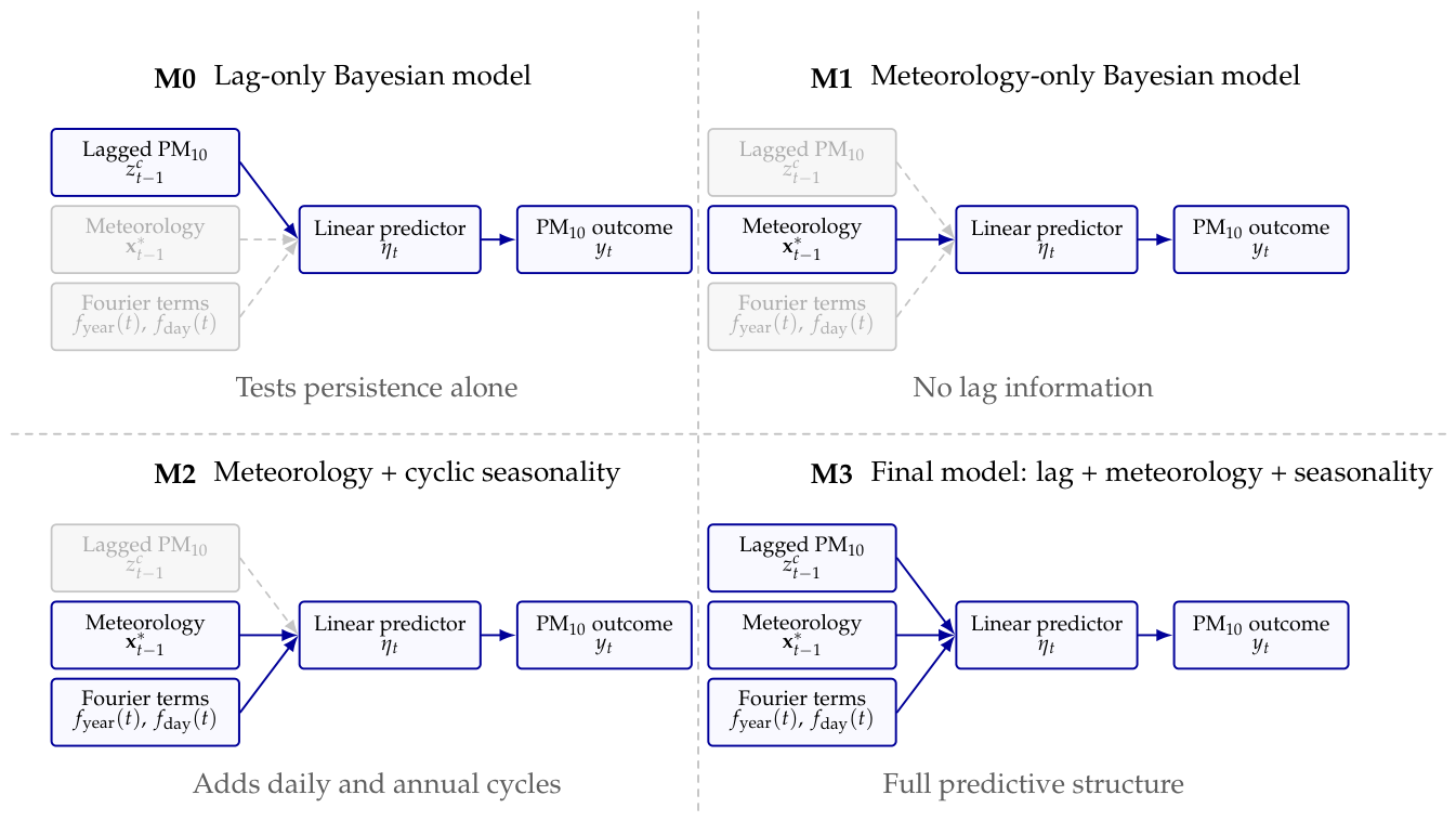
Figure 2.
Hourly concentrations and chronological evaluation structure. The top panel shows the full 2020–2024 series. The bottom panel shows the expanding training windows, four rolling-origin validation windows, and the final held-out test period.
Figure 2.
Hourly concentrations and chronological evaluation structure. The top panel shows the full 2020–2024 series. The bottom panel shows the expanding training windows, four rolling-origin validation windows, and the final held-out test period.
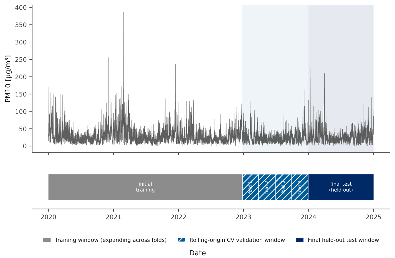
Figure 3.
Overall performance on the final test set. Filled dark markers denote the primary persistence-aware models; light markers denote secondary models. Gray ticks show mean rolling-origin cross-validation performance. The dashed line in the coverage panel marks the nominal 0.90 level.
Figure 3.
Overall performance on the final test set. Filled dark markers denote the primary persistence-aware models; light markers denote secondary models. Gray ticks show mean rolling-origin cross-validation performance. The dashed line in the coverage panel marks the nominal 0.90 level.
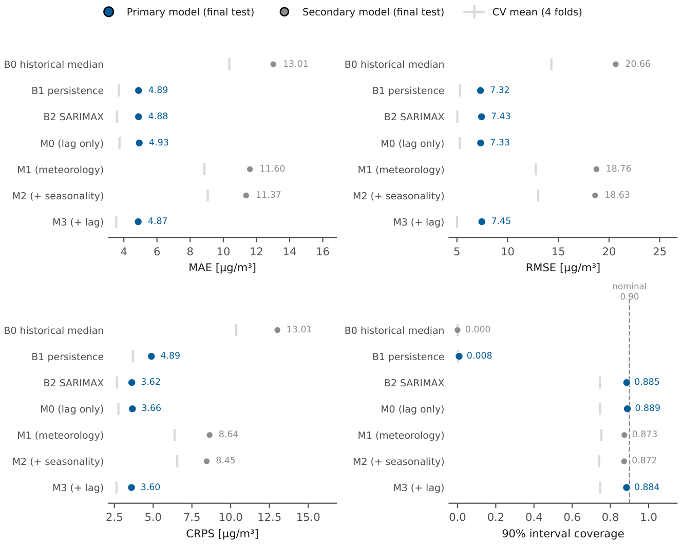
Figure 4.
PSIS-LOO comparison and Pareto-k diagnostics for the Bayesian models. The left panel shows expected log pointwise predictive density (elpd) differences relative to M3 with one-standard-error bars, while the right panel shows the maximum Pareto-k value for each model. Higher elpd indicates better predictive-density fit, and all Pareto-k values remain far below the usual warning threshold of 0.7.
Figure 4.
PSIS-LOO comparison and Pareto-k diagnostics for the Bayesian models. The left panel shows expected log pointwise predictive density (elpd) differences relative to M3 with one-standard-error bars, while the right panel shows the maximum Pareto-k value for each model. Higher elpd indicates better predictive-density fit, and all Pareto-k values remain far below the usual warning threshold of 0.7.
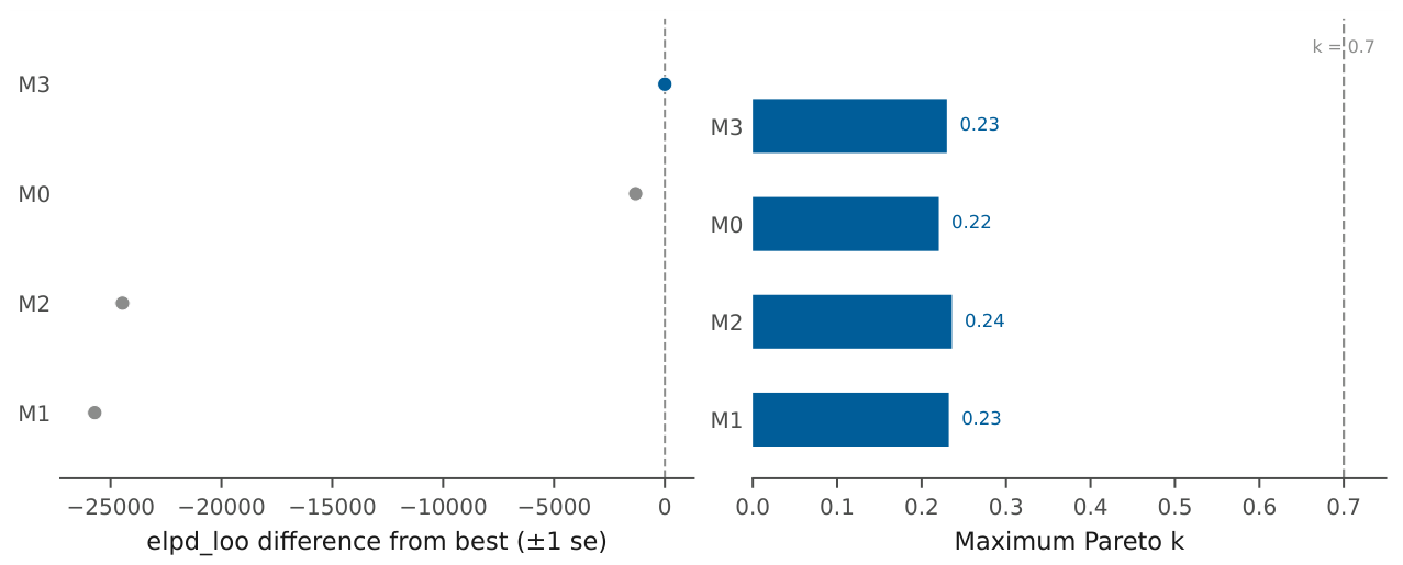
Figure 5.
Observed , M3 predictive median and 50%/90% intervals, and persistence forecast during 5–22 January 2024. The horizontal line marks the training-period 90th percentile used to define high-pollution hours.
Figure 5.
Observed , M3 predictive median and 50%/90% intervals, and persistence forecast during 5–22 January 2024. The horizontal line marks the training-period 90th percentile used to define high-pollution hours.
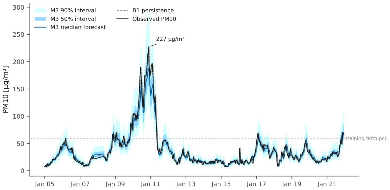
Figure 6.
Posterior median and 90% interval for multiplicative meteorological effects in M1 and M3. The vertical reference line denotes no effect.
Figure 6.
Posterior median and 90% interval for multiplicative meteorological effects in M1 and M3. The vertical reference line denotes no effect.
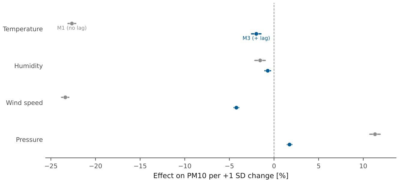
Figure 7.
MAE and RMSE on the full test set and on the high-pollution subset. Connected markers show how each primary model’s error changes when evaluation is restricted to hours above the training-period 90th percentile.
Figure 7.
MAE and RMSE on the full test set and on the high-pollution subset. Connected markers show how each primary model’s error changes when evaluation is restricted to hours above the training-period 90th percentile.
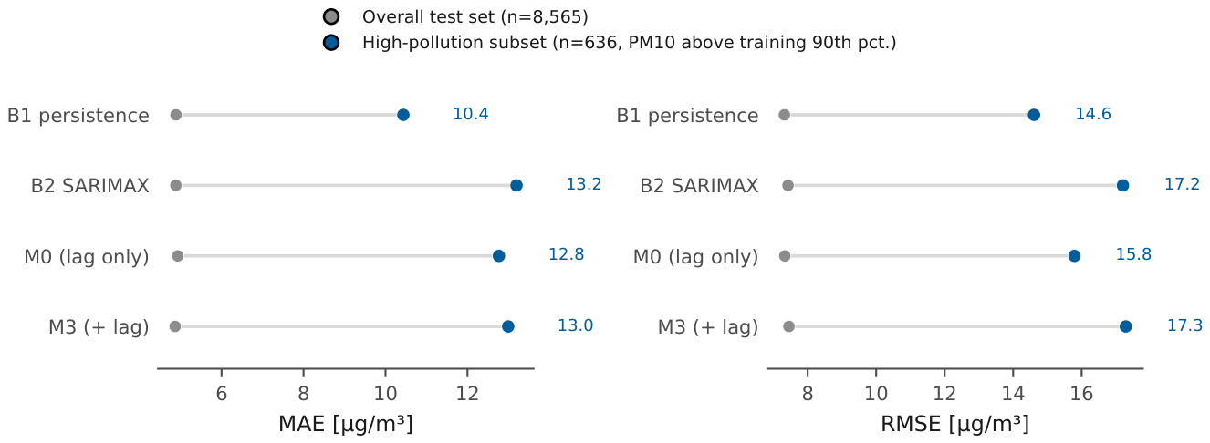

Table 1.
Data and split summary.
| Quantity | Value |
|---|---|
| Study period | 1 January 2020–31 December 2024 |
| Temporal resolution | Hourly |
| Model-ready observations | 42,823 |
| Final training set | 34,258 observations |
| Final held-out test set | 8565 observations |
| Rolling-origin validation folds | 4 |
| DST-ambiguous rows excluded | 10 rows; 0 weather rows |
| rows removed for missingness | 773 (1.76% of the complete hourly grid) |
| Target | concentration [] |
| Meteorological predictors | Temperature, relative humidity, wind speed, surface pressure; each lagged by 1 h |
| Additional inputs | Lagged log- (B1, B2, M0, M3); two annual and two daily Fourier harmonics (B2, M2, M3) |
Table 2.
Definitions of the reference and Bayesian models.
| ID | Model | Lag | Met. | Cyclic | Prob. | Definition |
|---|---|---|---|---|---|---|
| B0 | Historical median | – | – | – | – | Training-set median used for every hour. |
| B1 | Persistence | yes | – | – | – | . |
| B2 | SARIMAX | yes | yes | yes | yes | AR(1) dynamic regression on log-; rolling one-step Kalman forecasts. |
| M0 | Lag-only Bayesian | yes | – | – | yes | Lognormal model with centered lagged log-. |
| M1 | Meteorology-only Bayesian | – | yes | – | yes | Lognormal regression with standardized lagged meteorology. |
| M2 | Meteorology + seasonality | – | yes | yes | yes | M1 plus annual and daily Fourier terms. |
| M3 | Full Bayesian model | yes | yes | yes | yes | M2 plus centered lagged log-. |
Table 3.
Predictive performance on the final held-out test set ( hours). Lower MAE, RMSE, and CRPS are better. Coverage refers to the nominal 90% predictive interval. B0 and B1 are deterministic; their CRPS values correspond to point-mass forecasts and they do not provide predictive intervals.
Table 3.
Predictive performance on the final held-out test set ( hours). Lower MAE, RMSE, and CRPS are better. Coverage refers to the nominal 90% predictive interval. B0 and B1 are deterministic; their CRPS values correspond to point-mass forecasts and they do not provide predictive intervals.
| Model | MAE | RMSE | CRPS | Coverage | Width |
|---|---|---|---|---|---|
| B0 historical median | 13.013 | 20.661 | 13.013 | 0.000 | 0.000 |
| B1 persistence | 4.886 | 7.320 | 4.886 | 0.008 | 0.000 |
| B2 SARIMAX | 4.884 | 7.426 | 3.622 | 0.885 | 23.085 |
| M0 lag only | 4.930 | 7.332 | 3.659 | 0.889 | 23.894 |
| M1 meteorology | 11.605 | 18.757 | 8.641 | 0.873 | 50.322 |
| M2 + seasonality | 11.374 | 18.626 | 8.452 | 0.872 | 50.263 |
| M3 full | 4.865 | 7.453 | 3.602 | 0.884 | 22.957 |
Table 4.
Paired moving-block bootstrap comparison on the final test set (24 h blocks, 2000 replications). A negative difference favors the first model.
Table 4.
Paired moving-block bootstrap comparison on the final test set (24 h blocks, 2000 replications). A negative difference favors the first model.
| Comparison | Metric | Observed | Bootstrap median | 95% interval | |
|---|---|---|---|---|---|
| M3 vs B1 | MAE | -0.020 | -0.027 | [-0.141, 0.124] | 0.638 |
| M3 vs B1 | RMSE | 0.133 | 0.124 | [-0.256, 0.647] | 0.308 |
| M0 vs B1 | MAE | 0.044 | 0.043 | [-0.021, 0.134] | 0.107 |
| M0 vs B1 | RMSE | 0.013 | 0.007 | [-0.113, 0.188] | 0.460 |
| M3 vs M0 | CRPS | -0.057 | -0.057 | [-0.118, 0.015] | 0.941 |
| M3 vs M0 | MAE | -0.064 | -0.065 | [-0.156, 0.047] | 0.893 |
| M3 vs M0 | RMSE | 0.120 | 0.091 | [-0.217, 0.548] | 0.320 |
| M3 vs B2 | CRPS | -0.020 | -0.020 | [-0.046, 0.008] | 0.923 |
| M3 vs B2 | MAE | -0.018 | -0.018 | [-0.056, 0.025] | 0.792 |
| M3 vs B2 | RMSE | 0.027 | 0.024 | [-0.069, 0.145] | 0.326 |
| M0 vs B2 | CRPS | 0.037 | 0.038 | [-0.022, 0.086] | 0.090 |
Table 5.
Posterior multiplicative effect of a one-standard-deviation increase in each lagged meteorological predictor on median .
Table 5.
Posterior multiplicative effect of a one-standard-deviation increase in each lagged meteorological predictor on median .
| Predictor | Model | Median effect [%] | 90% interval [%] |
|---|---|---|---|
| Temperature | M1 | -22.65 | [-23.09, -22.21] |
| Temperature | M3 | -1.99 | [-2.52, -1.45] |
| Relative humidity | M1 | -1.55 | [-2.15, -0.98] |
| Relative humidity | M3 | -0.70 | [-1.02, -0.37] |
| Wind speed | M1 | -23.38 | [-23.80, -22.99] |
| Wind speed | M3 | -4.22 | [-4.48, -3.95] |
| Surface pressure | M1 | 11.32 | [10.73, 11.90] |
| Surface pressure | M3 | 1.74 | [1.48, 2.00] |
Disclaimer/Publisher’s Note: The statements, opinions and data contained in all publications are solely those of the individual author(s) and contributor(s) and not of MDPI and/or the editor(s). MDPI and/or the editor(s) disclaim responsibility for any injury to people or property resulting from any ideas, methods, instructions or products referred to in the content. |
© 2026 by the authors. Licensee MDPI, Basel, Switzerland. This article is an open access article distributed under the terms and conditions of the Creative Commons Attribution (CC BY) license (http://creativecommons.org/licenses/by/4.0/).
Copyright: This open access article is published under a Creative Commons CC BY 4.0 license, which permit the free download, distribution, and reuse, provided that the author and preprint are cited in any reuse.


