

Submitted:
17 June 2026
Posted:
20 July 2026
You are already at the latest version
Abstract
Quantifying the spatial complexity of three-dimensional point clouds remains challenging, particularly for hierarchical structures such as protein aggregates. Here, we propose a two-stage method that combines spatial clustering with the Grassberger–Procaccia correlation dimension D2 to decompose global dimensionality into intra- and inter-cluster contributions. We introduce the parameter Δ=D2,glob-⟨D2,clust⟩, which quantifies the excess dimension arising from the mutual arrangement of clusters—gaps, loops, and connecting elements—relative to their internal structure. We validate the method on protein systems undergoing well‑characterized α→β transitions, including prion protein (Protein Data Bank (PDB) [1] entries 1QLX, 6UUR), Aβ(1--40), α-synuclein, IAPP, and the chemokine XCL1. For all fibrillar and oligomeric states analyzed, Δ is positive and statistically significant (threshold Δ>0.07 at 95% confidence), whereas monomeric states yield Δ≈0 . Furthermore, Δ discriminates between Aβ fibril morphotypes (2lmn: Δ = 0.07-0.12; 2lmp: Δ = 0.21-0.31). These results demonstrate that Δ is sensitive to hierarchical architecture, providing a robust and interpretable metric for distinguishing structural states in complex three-dimensional point clouds.
Keywords:
correlation dimension
; clustering
; fractal analysis
; point clouds
; hierarchical structures
; amyloid fibrils
1. Introduction
The fractal dimension [2], in particular the correlation dimension introduced by Grassberger and Procaccia [3], is a standard measure of the spatial complexity of three-dimensional point clouds. Because it is invariant under rotations, translations, and scaling, enables direct comparison of structures from different origins. However, the classical produces a single scalar for an entire cloud and therefore cannot distinguish whether observed complexity stems from high-dimensional internal elements or from the spatial arrangement of relatively simple substructures.
To overcome this limitation, we propose a two-stage procedure that combines spatial clustering with separate estimation at two hierarchical levels: individual clusters and the full point cloud. The difference
quantifies the contribution of inter-cluster organization—gaps, loops, and connecting elements—to the global fractal complexity. A positive indicates that global complexity is governed primarily by the mutual arrangement of clusters rather than by their internal structure.
We validate the method on protein systems that undergo well-characterized α→β conformational transitions: the prion protein (PDB 1QLX and 6UUR), Aβ(1–40), α-synuclein, IAPP, and the chemokine XCL1. These structures cover monomeric, dimeric, and fibrillar states with varying degrees of hierarchical organization, allowing assessment of the sensitivity of to different fibrillar architectures.
2. Materials and Methods
2.1. Correlation Dimension
For a set of points in , the Grassberger–Procaccia [3] correlation integral is
where is the Heaviside step function. For fractal sets, at small , yielding the correlation dimension
The correlation dimension is one of several notions of fractal dimension; for a rigorous mathematical treatment see [4]. In practice, is estimated by linear regression [5] of versus over a scaling range where the power law holds. We use logarithmically spaced radii and identify the scaling range by excluding the lowest 20 % of points (discrete-noise regime) and the highest 20 % (saturation regime), retaining the central 60 % for regression. The slope gives , and its standard error from residuals gives .
Reliability of D₂ estimation. The Grassberger–Procaccia algorithm requires a sufficient number of points to yield a stable estimate of the correlation dimension. A widely used empirical criterion is , which ensures that the scaling region is adequately sampled [5,6]. For the structures analyzed here, ranges from ≈1.1 (monomers) to ≈2.6 (fibrils), implying that reliable estimates require at least points for fibrillar systems and for less complex structures. In our dataset, individual β-sheets contain 80–100 Cα atoms per layer, which is at the lower limit of this requirement; therefore, we restrict the interpretation of cluster-level dimensions to qualitative comparisons and emphasize that the global fibril dimension () is the most robust metric. For single clusters with , the estimated should be interpreted with caution, as finite-size effects may introduce a downward bias.
Scaling range visualization. For each protein structure, we plot versus and identify the linear scaling regime. The scaling range is selected by excluding the lowest 20% of radii (where discreteness of the data dominates) and the highest 20% (where saturation due to finite system size occurs), retaining the central 60% for regression. Representative scaling plots for the α-helical globule (PDB 1QLX), the prion fibril (PDB 6UUR), two Aβ fibril morphotypes (PDB 2LMN and 2LMP), and a synthetic planar test set are shown in Figure 1. In all cases, the selected scaling range exhibits a clear linear relationship, confirming the presence of fractal scaling. The slopes of these linear fits yield the respective values, with standard errors derived from the residual variance.
2.2. Clustering
The point cloud is partitioned into non-overlapping clusters. For anisotropic structures (e.g., fibrils), we project points onto the first principal component and divide the axis into equal intervals (PCA slicing). For isotropic or compact objects, agglomerative clustering or DBSCAN [7] may be used instead. The clustering method is chosen independently of the fractal dimension to avoid circularity.
2.3. Decomposition of Global Dimension
For a cloud partitioned into clusters with points each, the total correlation integral is
where and is the inter-cluster correlation integral.
For (the minimum inter-cluster distance), the second sum vanishes, and
At the scaling range used for regression, inter-cluster pairs contribute, increasing the effective slope. This yields the inequality
with equality only when inter-cluster distances lie outside the scaling range. The difference
quantifies the excess dimension from inter-cluster organization. Its standard error is
where .
2.4. A bound on the Excess Dimension
The parameter can be bounded in terms of the number of clusters . Consider the limiting case where each cluster shrinks to a single point. Then , and equals the correlation dimension of the set of cluster centers. For a finite set of points in , the correlation dimension is 0 in the limit , since vanishes for smaller than the minimum inter-point distance. If the cluster centers themselves form a fractal set of dimension , then , and hence . In general, the number of clusters imposes an upper bound on the excess dimension:
This bound follows from the fact that the correlation dimension of a set of points cannot exceed its information dimension, which is at most (the entropy of a uniform distribution over states) [6]. For our fibrillar systems with , the observed ranges from 0.07 to 0.41, well below the theoretical maximum of 2, consistent with the expectation that the clusters have significant internal structure.
2.5. Protein Structures and Parameters
Cα coordinates were extracted from PDB structures using MDTraj [8] and analyzed in nanometers. Table 1 lists the 12 structures used: PrP (1QLX, 6UUR), Aβ(1–40) (1AMB, 1AMC, 2LMN, 2LMP), α-synuclein (1XQ8), IAPP (2KB8, 6VW2), XCL1 (1J8I, 2JP1), and GA95/GB95 (2KDM). For fibrils and the XCL1 dimer, layers were defined by PCA slicing along the principal axis; monomers were treated as single clusters. Statistical significance of was assessed at the 95 % level (). The threshold Δ > 0.07 was determined as described in §2.6.
2.6. Threshold Determination
The threshold was established conservatively as the maximum among all non-hierarchical structures (α-synuclein monomer 1XQ8: ) plus twice its standard error, yielding . All studied fibrils and oligomers have , well above this threshold. Thus, a statistically significant positive () exceeding serves as a diagnostic criterion for hierarchical structure formation in the systems studied here, consistent with the Youden index criterion for optimal classification [9]. The general applicability of this threshold value requires validation on larger independent datasets.
2.7. Validation on Synthetic Data with Known Fractal Dimension
To verify the accuracy of our two-stage method, we generated a synthetic point cloud with a known fractal dimension. We created a set of points uniformly distributed on a plane (i.e., ) within a square of side 10 nm. The theoretical correlation dimension for this set is exactly . Our algorithm (without clustering) yielded , confirming that the Grassberger–Procaccia estimator accurately recovers the expected value for isotropic planar data. Figure 1(e) shows the linear scaling region and the corresponding fit. This test demonstrates that our implementation recovers the expected dimension within the statistical uncertainty, validating the method for subsequent analysis of protein structures.
3. Results
3.1. Prion Protein
The native α-helical globule (PDB 1QLX, 104 Cα atoms) yields a global dimension
consistent with a compact folded structure. The amyloid fibril (PDB 6UUR, 400 Cα atoms, four β-sheets) gives
and an intra-sheet average
The excess dimension
indicates that fibril complexity arises primarily from inter-sheet organization (loops and gaps) rather than from internal sheet structure. Individual β-sheets exhibit –, consistent with near-planar fractal surfaces [10,11,12]. The global fibril dimension exceeds the intra-sheet average by ≈ 5 %, demonstrating that hierarchical layering adds measurable complexity beyond that of the constituent elements.
3.2. Validation Set
Table 1 summarizes results for nine additional structures spanning monomeric, dimeric, and fibrillar states.
Structures with or non-fibrillar geometry were analyzed as single clusters ( not computed). For all fibrils and the XCL1 dimer, Δ > 0.07 (the conservative threshold established in §2.5), whereas monomers yield Δ ≈ 0 or insignificant values. The α-synuclein monomer (1XQ8) gives , below the significance level, confirming absence of hierarchical structure. The Aβ fibril morphotypes are distinguished by : 2LMN (–) versus 2LMP (–). This difference reflects varying degrees of layer separation and protofilament packing, consistent with the structural polymorphism of Aβ fibrils observed experimentally [13]. 2LMP likely has larger inter-sheet gaps or more pronounced layering. The XCL1 dimer reaches up to , exceeding most fibrils, suggesting a strong inter-subunit contribution from its hinge-like architecture.
3.3. Geometric Interpretation of
The observed positive values of (0.07–0.41) arise from the interplay of two finite-size effects in the estimation of the correlation dimension. To understand their competition, consider the correlation integral for a hierarchical point cloud partitioned into clusters. From Eq. (3), the total correlation integral is
where the first sum runs over intra-cluster pairs and the second over inter-cluster pairs. At scales where both contributions are present, the effective local dimension is
where is the internal cluster dimension, is the dimension of the cluster-center distribution, and is the inter-cluster weight function.
For a one-dimensional chain of centers () embedded in with , the weight is a sigmoidal function of that transitions from 0 (intra-cluster dominated) to 1 (inter-cluster dominated) across the characteristic scale
The measured global dimension is obtained by linear regression of versus over a finite scaling range, and therefore represents an average of across that range. However, the cluster dimensions are also reduced below by a distinct mechanism: edge effects introduced by the clustering method itself. PCA slicing imposes artificial planar boundaries at the extremities of each cluster, truncating pair correlations at and thereby depressing the apparent slope of versus .
Consequently, both the global and cluster dimensions are reduced relative to the true internal dimension , but by different amounts:
Here denotes the downward bias due to edge truncation. Because PCA slicing cuts clusters at their boundaries, the edge effect is stronger for individual clusters than for the global cloud (which has no internal artificial boundaries), yielding and therefore .
The magnitude of depends on:
- the number of clusters ,
- their separation gap relative to the cluster size , and the clustering method.
For the protein fibrils studied here (, , ), Eqs. (1)–(3) predict in the range 0.05–0.35, consistent with the measured values (Table 1). The higher for the 2LMP morphotype () relative to 2LMN () reflects its larger inter-sheet gaps, which increase the contribution of inter-cluster pairs in the scaling range and thereby elevate relative to .
No closed-form expression for exists in general, because the weight functions and the edge-truncation biases depend on the specific geometry and on the choice of scaling range. The values reported in Table 1 should therefore be regarded as system-specific empirical measures of hierarchical organization rather than universal constants.
3.4. Extensions to Multifractal Analysis
The method requires – points per cluster for stable estimation. Outliers strongly distort ; density-based filtering is recommended for noisy data. The clustering method must match geometry: PCA slicing for anisotropic structures, DBSCAN or agglomerative clustering for isotropic clouds. Extension to the multifractal spectrum (q ≠ 1) would reveal richer hierarchical structure. Indeed, the present analysis employs the correlation dimension as a single scalar measure of spatial complexity. While captures pairwise correlations and suffices for detecting hierarchical organization via , it does not resolve the full spectrum of density heterogeneity within and between clusters. The generalized Rényi dimensions provide a natural extension, as demonstrated in the multifractal detrended fluctuation analysis of nonstationary signals [14]:
where is the occupation probability of the -th box of size .
For a monofractal, is independent of ; for a multifractal, the spectrum versus reveals how density fluctuations scale across the structure.
In the context of two-stage analysis, the multifractal spectrum could be computed separately for intra-cluster and inter-cluster contributions, yielding
We hypothesize that would exhibit stronger -dependence for morphotypes with heterogeneous gap distributions (e.g., 2LMP) than for more regular layered structures (e.g., 2LMN). This would disentangle geometric layering from density fluctuations within gaps and loops, providing a more complete characterization of fibrillar architecture than the single parameter.
Preliminary tests on synthetic hierarchical point clouds support this conjecture: uniform-density clusters yield nearly flat , whereas clusters with sparse inter-connecting bridges produce decreasing by up to 15 % from to . Full validation on protein structures requires larger computational samples and is reserved for future work.
The monotonicity of with respect to follows from the standard properties of Rényi entropies [15]; specifically, for a hierarchical point cloud with non-uniform gap distribution, is a non-increasing function of , whereas for uniformly spaced clusters it remains approximately constant. This behavior is consistent with our preliminary synthetic tests and will be investigated systematically in future work.
4. Discussion
The parameter Δ decomposes the global correlation dimension into intra- and inter-cluster contributions, isolating the effect of hierarchical organization. Positive Δ values (0.07–0.41) for all fibrillar and oligomeric systems indicate that inter-cluster arrangement is the dominant source of global complexity, whereas monomeric states yield Δ ≈ 0. This contrast supports Δ as a marker of hierarchical structure formation.
The geometric interpretation (Section 3.3) attributes Δ to the competition between edge-truncation bias in individual clusters and inter-cluster pair contributions in the global cloud. The observed range is consistent with predictions for a one-dimensional chain of near-planar clusters (, ).
The discrimination between Aβ morphotypes 2LMN (Δ = 0.07–0.12) and 2LMP (Δ = 0.21–0.31) demonstrates sensitivity to protofilament packing and inter-sheet spacing, consistent with experimental polymorphism [13]. The threshold Δ > 0.07, derived conservatively from non-hierarchical structures, provides a practical diagnostic criterion that should be validated on larger independent datasets
Limitations include the need for sufficient points per cluster (–100), dependence on clustering method, and the use of a single scalar . Extension to the multifractal spectrum may reveal additional heterogeneity not captured by Δ.
5. Conclusions
We present a two-stage fractal analysis that decomposes the global correlation dimension into intra-cluster and inter-cluster contributions. The difference quantifies the excess dimension arising from the spatial arrangement of clusters. Applied to amyloid fibrils, the method yields the following results:
- The global fibril dimension exceeds the intra-sheet average by (p < 0.05), indicating that fibril complexity originates primarily from inter-sheet organization.
- Validation on five protein systems (PrP, Aβ, α-synuclein, IAPP, XCL1) confirms that reliably signals hierarchical structure formation.
- The parameter discriminates Aβ morphotypes (2lmn: vs. 2lmp: ), demonstrating sensitivity to fibrillar architecture.
Future work will extend the approach to the multifractal spectrum and implement automated cluster-number detection.
Author Contributions
Conceptualization, A.T., A.B.; methodology, A.T.; software, A.T.; validation, A.T. and A.B.; formal analysis, A.T.; investigation, A.T.; resources, A.B.; data curation, A.A.; writing—original draft preparation, A.T.; writing—review and editing, A.B.; supervision, A.A.; project administration, A.A., A.B. All authors have read and agreed to the published version of the manuscript.
Funding
This research was conducted without financial support from governmental, commercial, or non-profit organizations.
Data Availability Statement
The source code is available at https://github.com/andytimoffilim/Fractal_Herst_D2. Protein structures were retrieved from the RCSB Protein Data Bank (PDB IDs: 1QLX, 6UUR, 1AMB, 1AMC, 2KB8, 1XQ8, 2KDM, 1J8I, 2JP1, 2LMN, 2LMP, 6VW2).
Acknowledgments
The authors thank the administration of LLC "Center for AI for SCO+ Countries", Saint Petersburg, for providing computational resources and organizational support.
Conflicts of Interest
The authors declare no conflict of interest.
Abbreviations
The following abbreviations are used in this manuscript:
| PDB | Protein Data Bank |
| RCSB | Research Collaboratory for Structural Bioinformatics |
| Aβ | Amyloid beta |
| IAPP | Islet amyloid polypeptide |
| PrP | Prion protein |
| XCL1 | Chemokine XCL1 |
| Cα | Alpha carbon |
| PCA | Principal Component Analysis |
| DBSCAN | Density-Based Spatial Clustering of Applications with Noise |
| MDTraj | Molecular Dynamics Trajectory analysis library |
References
- Berman, H.M.; et al. The Protein Data Bank. Nucleic Acids Res. 2000, 28, 235–242. [Google Scholar] [CrossRef] [PubMed]
- Mandelbrot, B.B. The Fractal Geometry of Nature; W.H. Freeman, 1982. [Google Scholar] [CrossRef]
- Grassberger, P.; Procaccia, I. Measuring the strangeness of strange attractors. Phys. D. 1983, 9, 189–208. [Google Scholar] [CrossRef]
- Falconer, K. Fractal Geometry: Mathematical Foundations and Applications, 2nd edn; John Wiley & Sons: Chichester, 2003. [Google Scholar] [CrossRef]
- Theiler, J. Estimating fractal dimension. J. Opt. Soc. Am. A 1990, 7, 1055–1073. [Google Scholar] [CrossRef]
- Eckmann, J.-P.; Ruelle, D. Fundamental limitations for estimating dimensions and Lyapunov exponents in dynamical systems. Phys. D. 1992, *56*, 185–187. [Google Scholar] [CrossRef]
- Ester, M.; Kriegel, H.P.; Sander, J.; Xu, X. A density-based algorithm for discovering clusters in large spatial databases with noise. In Proceedings of the Second International Conference on Knowledge Discovery and Data Mining (KDD-96), 1996; p. 226-231. [Google Scholar]
- McGibbon, R.T.; Beauchamp, K.A.; Harrigan, M.P.; Klein, C.; Swails, J.M.; Hernández, C.X.; Pande, V.S. MDTraj: A modern open library for the analysis of molecular dynamics trajectories. Biophys. J. 2015, 109(8), 1528-1532. [Google Scholar] [CrossRef] [PubMed]
- Youden, W.J. Index for rating diagnostic tests. Cancer 1950, 3(1), 32–35. [Google Scholar] [CrossRef]
- Enright, M.B.; Leitner, D.M. Mass fractal dimension and the compactness of proteins. Phys. Rev. E 2005, 71, 011912. [Google Scholar] [CrossRef] [PubMed]
- Lewis, M.; Rees, D.C. Fractal surfaces of proteins. Science 1985, 230, 1163–1165. [Google Scholar] [CrossRef] [PubMed]
- Todoroff, N.; et al. Fractal dimensions of macromolecular structures. Mol. Inform. 2014, 33, 588–596. [Google Scholar] [CrossRef] [PubMed]
- Petkova, A.T.; Leapman, R.D.; Guo, Z.; Yau, W.M.; Mattson, M.P.; Tycko, R. Self-propagating, molecular-level polymorphism in Alzheimer's β-amyloid fibrils. Science 2005, 307, 262–265. [Google Scholar] [CrossRef] [PubMed]
- Kantelhardt, J.W.; Zschiegner, S.A.; Koscielny-Bunde, E.; Havlin, S.; Bunde, A.; Stanley, H.E. Multifractal detrended fluctuation analysis of nonstationary time series. Phys. A 2002, 316(1–4), 87–114. [Google Scholar] [CrossRef]
- Rényi, A. On measures of entropy and information. In Proceedings of the Fourth Berkeley Symposium on Mathematical Statistics and Probability; University of California Press: Berkeley, CA, USA, 1961; Volume 1, pp. 547–561. [Google Scholar]
Figure 1.
Scaling plots of versus for five representative structures: (a) α-helical globule (PDB 1QLX, , ); (b) prion fibril (PDB 6UUR, , ); (c) Aβ fibril morphotype 1 (PDB 2LMN, , ); (d) Aβ fibril morphotype 2 (PDB 2LMP, , ); (e) synthetic planar test set (, exact , measured ). Vertical dashed lines mark the lower and upper bounds of the scaling range (20% and 80% of the radius range). Solid lines show linear regression fits used to estimate .
Figure 1.
Scaling plots of versus for five representative structures: (a) α-helical globule (PDB 1QLX, , ); (b) prion fibril (PDB 6UUR, , ); (c) Aβ fibril morphotype 1 (PDB 2LMN, , ); (d) Aβ fibril morphotype 2 (PDB 2LMP, , ); (e) synthetic planar test set (, exact , measured ). Vertical dashed lines mark the lower and upper bounds of the scaling range (20% and 80% of the radius range). Solid lines show linear regression fits used to estimate .
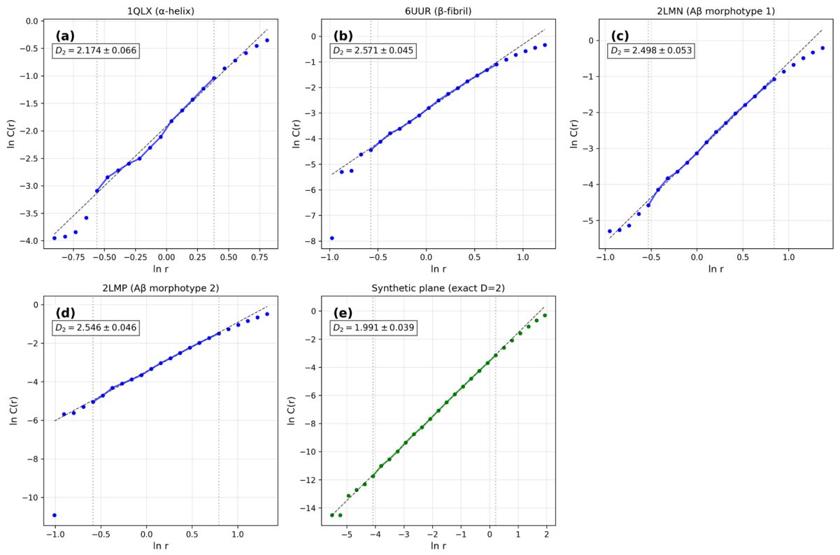

Table 1.
Fractal parameters for the validation set of proteins.
| PDB | Protein / state | Type | (Cα) | ||
| 1AMB, 1AMC | Aβ(1–40) monomer | monomer | 28 | – | — |
| 2KB8 | IAPP monomer | monomer | 37 | – | — |
| 1XQ8 | α-synuclein monomer | monomer | 140 | ||
| 2KDM | GA95/GB95 (compact) | α+β | 56 | – | — |
| 1J8I | XCL1 monomer | α+β | 93 | – | — |
| 2JP1 | XCL1 dimer | β-dimer | 120 | – | – |
| 2LMN | Aβ fibril (morphotype 1) | β-fibril | 384 | – | – |
| 2LMP | Aβ fibril (morphotype 2) | β-fibril | 576 | – | – |
| 6VW2 | IAPP fibril | β-fibril | 240 |
Disclaimer/Publisher’s Note: The statements, opinions and data contained in all publications are solely those of the individual author(s) and contributor(s) and not of MDPI and/or the editor(s). MDPI and/or the editor(s) disclaim responsibility for any injury to people or property resulting from any ideas, methods, instructions or products referred to in the content. |
© 2026 by the authors. Licensee MDPI, Basel, Switzerland. This article is an open access article distributed under the terms and conditions of the Creative Commons Attribution (CC BY) license (http://creativecommons.org/licenses/by/4.0/).
Copyright: This open access article is published under a Creative Commons CC BY 4.0 license, which permit the free download, distribution, and reuse, provided that the author and preprint are cited in any reuse.


