

Submitted:
16 July 2026
Posted:
20 July 2026
You are already at the latest version
Abstract
The integration of photovoltaic (PV) generation into power systems requires design methods that evaluate not only annual energy yield or installed capacity, but also the dependable contribution of the plant under critical supply conditions. This paper presents a prototype-driven methodology for the physical validation and optimal sizing of a grid-connected PV generation system aimed at estimating, auditing, and evaluating ENFICC-oriented photovoltaic sizing alternatives under the Colombian reliability framework. The workflow integrates three input databases: a ten-year hourly meteorological database from NASA POWER for 2016--2025, a filtered and expanded PV module catalog based on the CEC database, and a filtered and expanded inverter catalog based on the Sandia database. These inputs feed a sequential modeling chain that estimates clearness index, irradiance decomposition, plane-of-array irradiance, cell temperature, DC power, AC power, monthly equivalent daily energy, net effective capacity, regulatory upper bound, and final ENFICC. The methodology was first validated using the installed PV system in La Tebaida, Colombia, as a local physical reference. For the validation case, the model used 252 Jinko Tiger Neo JKM625N-78HL4-BDV modules, two Solis 60K-LV-5G inverters, 157.5 kWp DC, 120 kW AC, fixed topology, and an hourly local validation dataset derived from the installed system. The NASA-based physical validation produced a critical-month energy of 548.5~kWh/day and a final ENFICC of 438.8~kWh/day after applying the secondary-data factor \(f_{\mathrm{sec}}=0.8\). After applying the corrected physical filters and monthly coverage checks to the NASA POWER physical irradiance series, ten independent GA runs produced final ENFICC values between 283.5 and 384.2 kWh/day, with a mean of 349.7 kWh/day. The fitness function in all GA runs was evaluated using the corrected NASA POWER physical irradiance series, not an alternative irradiance series. These corrected results do not support the previously inflated optimization values; instead, they show that the local physical validation stage is essential before interpreting GA outputs. The proposed methodology contributes to clean-energy planning by linking renewable-energy integration, physical validation, reproducible computation, and regulatory firm-energy estimation within a single engineering workflow.
Keywords:
firm energy
; ENFICC
; photovoltaic systems
; optimal sizing
; physical validation
; genetic algorithm
; solar irradiance
; reliability charge
; NASA POWER
; clean energy
; La Tebaida
1. Introduction
The transition toward low-carbon energy systems has accelerated the deployment of photovoltaic (PV) generation in distribution and transmission networks. PV technology offers modularity, decreasing investment costs, and broad resource availability, which makes it a central option for clean-energy expansion and decarbonization [1,2]. Nevertheless, high penetration of variable renewable generation also creates technical and market challenges associated with resource variability, system adequacy, operational planning, dispatchability, and the definition of dependable capacity contributions.
In Colombia, centrally dispatched generators participate in a reliability mechanism through the Firm Energy Obligation (Obligacion de Energia Firme, OEF). Under this framework, each plant must determine its Firm Energy for the Reliability Charge (Energia Firme para el Cargo por Confiabilidad, ENFICC), which represents the energy contribution that the asset can support under critical supply conditions [3]. Although ENFICC is a Colombian regulatory concept, the engineering problem is broader: it is equivalent to estimating the reliability contribution of a variable renewable plant within a firm-energy or capacity-remuneration framework. Therefore, ENFICC can be interpreted as a market-specific metric of dependable renewable generation.
For solar PV plants, ENFICC estimation is more demanding than for conventional thermal units because the available energy depends on the long-term variability of irradiance, ambient temperature, PV conversion efficiency, inverter operation, losses, availability, and the selected plant configuration. CREG Resolution 101 007 of 2023 requires hourly historical series of global horizontal irradiance and ambient temperature, with at least ten years of information and at least one year of on-site measurements when available [4]. When only secondary data are used, the calculated ENFICC must be adjusted using the correction factor established by the applicable regulation [5]. This requirement makes data traceability and methodological reproducibility central elements of the sizing process.
The literature on PV sizing has traditionally focused on installed capacity, annual generation, loss reduction, voltage profiles, LCOE, cost minimization, or hybrid-system reliability [6,7,8,9]. In Energies, recent studies have optimized PV placement and sizing under spatial constraints, addressed hybrid-system sizing for the Colombian context using GA and PSO, and developed optimal sizing approaches for PV/BESS systems in substation auxiliary services [10,11,12]. These works confirm the relevance of metaheuristic optimization for PV planning, but their objectives differ from a firm-energy-oriented regulatory criterion.
Complementary clean-technology studies have also optimized hybrid renewable-energy systems using PSO and multi-criteria formulations that combine cost, reliability, and renewable fraction [13]; analyzed on–off-grid hybrid systems with PV, wind, and batteries under reliability and economic constraints [14]; and proposed hybrid microgrid designs that explicitly compare PV tilt and azimuth alternatives while evaluating cost and CO2 emissions [15]. Other contributions have used reliability indices such as loss-of-load probability in PV-based hybrid systems [16]. These studies support the methodological relevance of optimization and clean-energy planning, but they do not formulate the PV sizing problem as the maximization of firm energy under a reliability-charge mechanism.
This paper addresses that gap by developing a prototype-driven methodology that links input databases, PV physical equations, local validation, and a genetic algorithm (GA) to evaluate ENFICC-oriented PV sizing alternatives. The main contribution is not an unconditional increase in ENFICC, but an auditable workflow that first validates the physical energy scale of the installed system and then evaluates whether catalogue-based GA alternatives can improve, match, or challenge that validated baseline. In this formulation, the design is governed by the worst-performing month, the regulatory upper bound, the secondary-data correction factor, the available land area, and the technical compatibility between modules and inverters. The case study is centered on the installed PV system in La Tebaida, Colombia, which is used as the physical reference before interpreting the independent GA design-search results.
The specific contributions of this paper are: (i) a structured description of the meteorological, module, and inverter databases used by the computational prototype; (ii) a sequential equation-based modeling chain from GHI to final ENFICC; (iii) a local physical-validation stage using the installed La Tebaida PV system; (iv) a mixed discrete–continuous GA for ENFICC-oriented PV sizing evaluated through ten independent runs; and (v) an equation-level graphical audit showing how physical filters, inverter-energy protection, and monthly-coverage checks prevent unrealistic ENFICC improvements from being accepted.
The remainder of the paper is organized as follows. Section 2 presents the input databases, modeling equations, and GA structure. Section 3 reports the results for the La Tebaida case study, emphasizing the corrected meteorological dataset, the local physical validation, and the equation-level analysis of independent GA runs. Section 4 discusses the implications of the corrected results for the installed system, ENFICC-oriented PV assessment, and clean-energy planning. Section 5 presents the conclusions.
2. Materials and Methods
2.1. Computational Prototype and Input Databases
The meteorological database serves as the first layer of information in the proposed automated PV sizing approach, as the FE-oriented objective function depends directly on the hourly representation of the solar resource and ambient operating conditions. Hourly data were obtained from the NASA POWER database through its API service for the 2016–2025 period. The extracted variables were ALLSKY_SFC_SW_DWN, used as global horizontal irradiance (GHI) for PV performance calculations; T2M, corresponding to ambient temperature at 2 m; and RH2M, corresponding to relative humidity at 2 m. These variables provide the minimum meteorological information required to estimate the plane-of-array irradiance, determine the cell temperature, and calculate the hourly AC energy output of each candidate PV configuration. The use of a single corrected physical irradiance series also ensures that all candidate designs are evaluated under identical solar-resource conditions.
The case study corresponds to the installed PV system in La Tebaida, Quindio, Colombia, located at latitude N, longitude W, and an elevation of approximately 1500 m a.s.l. This geographic location was used to query the NASA POWER data and to define the solar-geometry calculations used throughout the PV performance model. At this location, the raw dataset contains 87,672 hourly records, corresponding to a continuous ten-year UTC series that was converted to the America/Bogota working time zone for the subsequent PV simulation. The preprocessing stage first verified the temporal continuity of the hourly index to prevent missing or duplicated timestamps from propagating into the energy calculation. Physical consistency checks were then applied to the irradiance series, including detection of negative and non-physical values, as well as night-time GHI inconsistencies based on the solar zenith angle. When required, irradiance values outside physically admissible ranges were clipped or corrected before calculating the direct, diffuse, and plane-of-array irradiance components.
The cleaned meteorological database was used consistently in all stages of the computational workflow, including irradiance transposition, PV performance modeling, local validation, ENFICC calculation, and automated sizing. No statistical, data-driven, forecasted, or alternative irradiance series was used as an input to the optimization process. Therefore, the FE-oriented objective function was evaluated exclusively using the corrected NASA POWER physical irradiance series. This convention avoids inconsistencies that would arise if different solar-resource series were used for validation, energy conversion, and sizing. It also makes the comparison among candidate PV configurations dependent on design decisions and physical constraints rather than on changes in the irradiance input.
The available installation surface was represented as a rectangular area of 32 m × 33 m. A 1.0 m perimeter margin was excluded from this area to account for practical spacing and accessibility requirements, yielding a net usable area of approximately 969.8 m2. This net area was imposed as a geometric constraint during the evaluation of candidate PV layouts. The resulting spatial representation is consistent with prototype-level PV sizing studies in which the optimal configuration is constrained by land availability, module dimensions, tilt angle, azimuth angle, and inverter compatibility [14,15]. Thus, the sizing process combines meteorological, electrical, and geometric information within a single reproducible computational framework.
The second information layer corresponds to the photovoltaic module database used to define the discrete component alternatives available to the automated PV sizing approach. This catalog was derived from the California Energy Commission (CEC) database and filtered to retain commercially relevant crystalline-silicon modules compatible with the technical ranges required for ENFICC-oriented PV-system modeling. The filtering criteria included monocrystalline technology, nominal STC power above 350 W, feasible module area, complete electrical parameters, a negative temperature coefficient of maximum power, and exclusion of building-integrated photovoltaic modules. After filtering, 977 modules remained from the original source database. Eight additional high-power bifacial modules representative of the 2024-2025 commercial market were manually incorporated to extend the upper range of available module ratings. The resulting expanded database contains 985 PV modules from 58 manufacturers, with an availability period spanning 2019-2024.
The technical attributes retained from the module database were selected based on their roles in the PV performance model and the feasibility constraints of the automated sizing procedure. For each candidate module, the workflow used the nominal power at standard test conditions, , the voltage and current at the maximum power point, and , the open-circuit voltage, , the physical module area, and the estimated conversion efficiency. These variables determine the DC capacity of each candidate layout, the string-level voltage and current limits, the land-use constraint, and the expected energy yield under the corrected NASA POWER irradiance series. Therefore, the sizing procedure does not rely on an abstract or continuous module model, but on a traceable set of commercially available component alternatives. This design choice is relevant because the best achievable ENFICC value is constrained by the technical diversity and parameter boundaries of the component database. Consequently, expanding and documenting the module catalog contributes directly to the reproducibility of the proposed sizing methodology.
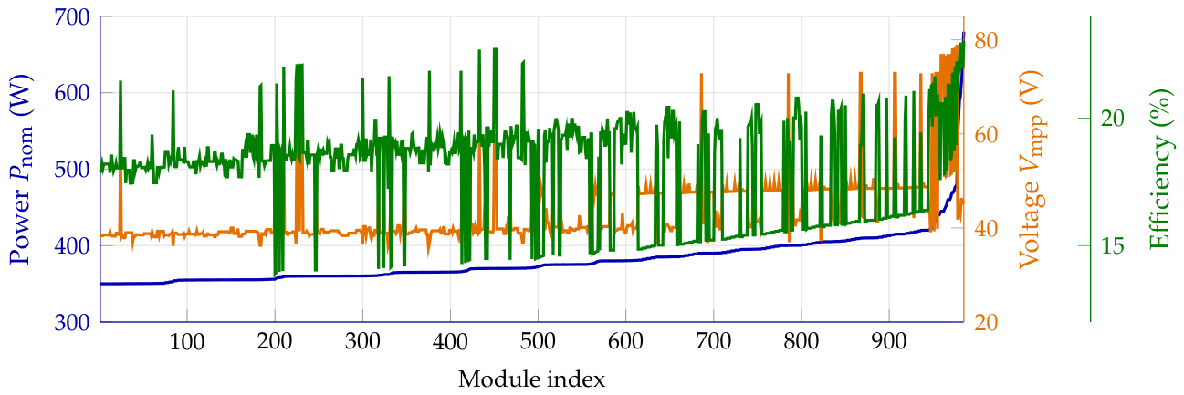
Figure 1 summarizes the numerical span of the filtered and expanded PV module database. The range plot is included immediately after the module-database description to make explicit the module search space available to the automated sizing procedure before the optimization results are presented. The expanded database covers STC powers from 350.0 to 680.0 W, module areas from 1.63 to 2.98 m2, and estimated efficiencies from 13.89% to 23.04%. This range allows the decision variables to span compact high-efficiency modules, intermediate alternatives, and larger high-power modules under the same land, electrical, and inverter-compatibility constraints. As a result, the selected module is not imposed a priori, but emerges from the interaction between the component database, the corrected physical irradiance input, the feasibility constraints, and the ENFICC-oriented objective function.
Figure 1.
Operating ranges of the photovoltaic module database used in the genetic algorithm. The curves represent the nominal power, maximum power point voltage, and estimated efficiency for each module in the dataset.
Figure 1.
Operating ranges of the photovoltaic module database used in the genetic algorithm. The curves represent the nominal power, maximum power point voltage, and estimated efficiency for each module in the dataset.
The third information layer corresponds to the inverter database, which defines the discrete set of AC conversion technologies available to the automated PV sizing approach. This catalog was constructed from the Sandia inverter database and subsequently filtered according to AC power rating, maximum DC voltage limit, MPPT operating window, maximum DC current capability, and parameter-validity criteria. The resulting database contains 222 inverter entries from 40 manufacturers, with an availability period spanning 2018–2024. Five additional commercial inverter models with high market penetration in Colombia were included to improve the representativeness of the search space for local PV applications. Among these models, the Solis 60K-LV-5G was retained because it matches the inverter used in the La Tebaida validation case and is therefore a relevant feasible alternative among the candidate configurations. The final inverter database covers nominal AC power ratings from 15 to 200 kW, which is suitable for the PV system scale evaluated in this study.
The technical attributes retained from the inverter database were selected based on their roles in the electrical-feasibility constraints and the AC energy-conversion model. For each candidate inverter, the workflow used the nominal AC power, , the maximum admissible DC voltage, , the MPPT voltage range, and the maximum DC current. These parameters determine whether the voltage and current produced by a candidate module-string configuration are compatible with the selected inverter. They also define the admissible DC/AC ratio, the onset of AC clipping, and the maximum AC power that each candidate plant layout can inject. Therefore, the automated sizing procedure does not select an inverter from an abstract capacity interval, but from a traceable database of technically feasible commercial devices. This formulation ensures that the sizing process simultaneously accounts for energy yield, electrical compatibility, and component-level implementation constraints.
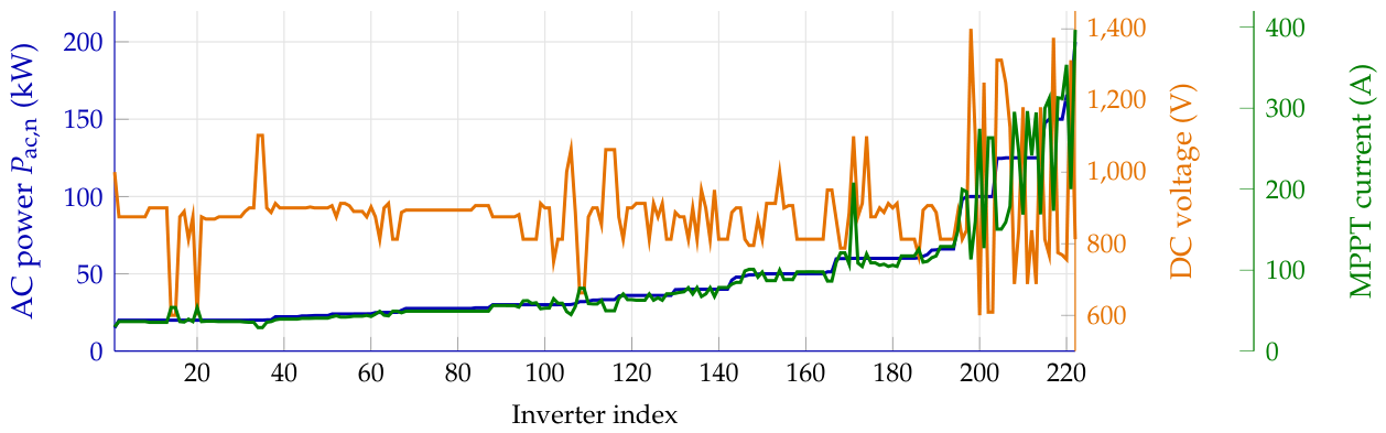
Figure 2 presents the numerical range of the filtered and expanded inverter database. The range plot is included immediately after the inverter-database description to make explicit the electrical search space available to the automated sizing procedure. The database spans nominal AC powers from 15.0 to 200.0 kW and DC power ratings from 15.46 to 206.26 kW. In addition, the MPPT voltage windows cover a broad operating region, allowing the sizing procedure to evaluate different string lengths and module-inverter pairings under realistic voltage constraints. This inverter parameterization is relevant because compatibility must be verified before calculating hourly AC generation and the resulting FE-oriented objective value. Consequently, the selected inverter emerges from the interaction between the module database, the corrected NASA POWER irradiance input, the electrical constraints, and the objective of maximizing firm energy.
Figure 2.
Operating ranges of the inverter module database used in the genetic algorithm. The curves represent the nominal AC power, maximum DC voltage, and maximum MPPT current for each module in the dataset.
Figure 2.
Operating ranges of the inverter module database used in the genetic algorithm. The curves represent the nominal AC power, maximum DC voltage, and maximum MPPT current for each module in the dataset.
2.2. Photovoltaic and Firm Energy Modeling Framework
The proposed methodology represents the photovoltaic (PV) plant as a sequential conversion process in which the available solar resource is transformed into hourly AC generation. Subsequently, the Firm-Energy (FE) indicator results from the simulated PV generation profile and the applicable regulatory constraints. The modeling sequence characterizes the atmospheric conditions associated with the hourly irradiance input, estimates the irradiance incident on the PV plane, converts this irradiance into DC and AC power, and evaluates the resulting monthly energy profile through a critical-month criterion. This formulation allows the automated PV sizing approach to compare candidate configurations based on their contribution during the most restrictive month, rather than only maximizing annual energy production.
The first step in the sequential conversion estimates the clearness index, , which quantifies the fraction of extraterrestrial solar irradiance that reaches the site on a horizontal plane. This index is calculated as the ratio between the global horizontal irradiance and the extraterrestrial normal irradiance projected onto the horizontal plane:
where t denotes the hourly simulation step, the global horizontal irradiance, and the solar zenith angle. The term corresponds to the extraterrestrial normal irradiance associated with the day of the year corresponding to each hourly record. Thus, hourly variables such as and vary within the day, whereas the extraterrestrial correction varies with the day index n. The hour-day relation maps each hourly timestamp to its corresponding day of the year. The extraterrestrial normal irradiance is calculated using the eccentricity correction associated with the annual variation in the Earth–Sun distance:
being the solar constant and n the day of the year. The coefficient approximates the annual eccentricity effect, and the denominator 365 defines the yearly periodicity used in the implementation. Consequently, Equation (1) compares the measured or estimated irradiance at the site with the extraterrestrial irradiance available under the same solar-position conditions.
Given , the global horizontal irradiance decomposes into diffuse horizontal irradiance and direct normal irradiance . This decomposition allows tilted PV modules to receive direct, diffuse, and ground-reflected irradiance components with different geometric factors according to the Erbs correlation from the clearness index [17]:
The irradiance components are then obtained as:
with denoting the empirical diffuse-fraction model. The decomposition is applied only under daylight conditions to avoid numerical instabilities when approaches zero, hence mitigating errors in and that propagate to the plane-of-array irradiance and, consequently, to monthly AC generation. This effect may be significant during cloudy periods, which can determine the critical-month value used in the FE-oriented objective function.
The irradiance incident on the tilted PV plane is estimated as the sum of beam, sky-diffuse, and ground-reflected components. In this implementation, an isotropic sky transposition model is adopted. The resulting plane-of-array irradiance, , is given by:
where estimates the beam transposition ratio from the incidence angle on the module surface and the solar zenith angle . corresponds to the module tilt angle. The terms and represent the isotropic sky-view and ground-view factors, respectively. The parameter denotes ground albedo. Here, is adopted when site-specific albedo measurements are unavailable to represent a generic ground-reflection condition. Since denotes the irradiance received by the module plane, this stage links array orientation, tilt, and topology with the monthly energy profile used by the automated PV sizing approach.
Numerical and physical safeguards were applied before converting irradiance into electrical power. Negative irradiance values were clipped to zero, and irradiance decomposition was applied only when . The beam transposition ratio was evaluated only under valid daylight and front-side incidence conditions; otherwise, the beam contribution was set to zero. Non-finite values of , , , , or the incidence-angle modifier were replaced by zero. In addition, monthly FE calculations retained only months satisfying the minimum data-coverage threshold defined in the implementation. In this work, months with at least 99% hourly coverage were retained for the critical-month calculation, thereby preventing incomplete edge months from controlling the FE estimate.
It is worth noting that the irradiance received by the module is not converted into electrical power under ideal thermal conditions. Part of the incident energy increases the module temperature, and higher cell temperature reduces the power output of crystalline-silicon PV modules. Hence, the cell temperature is estimated using the Faiman model:
being the cell temperature, the ambient temperature, and the wind speed, respectively. The coefficients and represent the thermal exchange between the module and the surrounding environment. The former captures the basic heat-loss mechanism, whereas the latter accounts for the additional cooling effect of wind. When local wind measurements are unavailable, the model assumes to maintain numerical consistency.
In addition to thermal effects, the proposed PV generation model also considers optical losses caused by non-normal solar incidence, which are parameterized by the incidence-angle modifier . Particularly, the formulation from the American Society of Heating, Refrigerating and Air-Conditioning Engineers (ASHRAE) is adopted:
with coefficient approximating the increase in reflection losses as the incidence angle increases. A default is used when module-specific optical characterization is unavailable. The optical correction is applied only for valid front-side incidence conditions and is clipped to non-negative values to avoid non-physical optical gains or losses at extreme incidence angles. Although early-morning and late-afternoon hours usually have lower irradiance, their cumulative contribution may affect the monthly energy profile. Therefore, including improves the physical consistency of the FE-oriented PV performance model.
Once the irradiance, temperature, and optical effects are defined, the DC power produced by the PV array is estimated as:
being the installed DC capacity under Standard Test Conditions, the reference irradiance, and the reference cell temperature. The coefficient stands for the module power temperature coefficient, obtained from the manufacturer’s datasheet or module database. Since the temperature coefficient is typically negative for crystalline-silicon modules, increases in cell temperature reduce . The term represents DC-side losses, including wiring, mismatch, and other losses not explicitly resolved in the prototype implementation. In this formulation, and are both expressed in watts.
Subsequently, a central calculation stage converts the DC power into net AC power through the inverter system. This stage accounts for inverter conversion efficiency, AC clipping, AC-side losses, and transformer losses:
where corresponds to the DC power assigned to inverter j, denotes the inverter efficiency, stands for the nominal AC rating of inverter j, and indicates the number of inverters in the plant. The minimum operator prevents inverter output from exceeding either the converted DC power or the nominal AC rating. The loss factors and represent AC-side and transformer losses, respectively. Here, constant inverter efficiency is used as a reduced-order approximation when a detailed inverter efficiency curve is unavailable to preserve the main effects of inverter conversion and AC clipping while maintaining computational efficiency during the automated sizing process. If manufacturer-specific efficiency curves are available, is replaced by a load-dependent inverter model.
2.3. Genetic Algorithm Formulation
The PV sizing problem involves continuous (e.g., tilt angle, azimuth angle, DC/AC ratio), discrete (e.g., number of series and parallel components), and categorical (e.g., module selection, inverter selection, topology) decision variables. Therefore, each candidate solution encodes the selected PV module from the expanded CEC-based database, the selected inverter from the expanded SANDIA-based database, the array topology, the DC/AC ratio, the installation angles, and the feasible number of modules and inverters. Candidate configurations are evaluated using the equivalent daily energy of the worst-performing month as the fitness function, as described in Equation (10). Infeasible solutions, including those that violate land-use or component-compatibility constraints, receive a near-zero fitness value. Although other population-based metaheuristics, such as particle swarm optimization (PSO), differential evolution (DE), and NSGA-II, have demonstrated strong performance in renewable-energy optimization [11,13], the present work selects the Genetic Algorithm (GA) as the solver for the PV sizing problem because its chromosome representation naturally accommodates mixed discrete–continuous decision variables and discrete catalogue-based component selection without requiring gradient information, making it well suited to the proposed prototype.
Figure 3 summarizes the architecture of the implemented GA. The workflow begins with the admissible design space defined by the corrected NASA POWER physical irradiance series, the filtered equipment databases, the land-use constraint, and the ENFICC regulatory requirements. Each chromosome represents a complete PV plant configuration and is evaluated through the irradiance-processing chain, PV performance equations, electrical compatibility checks, and the ENFICC objective function. The evolutionary cycle then applies selection, crossover, mutation, elitism, and replacement until the stopping criterion is reached. The GA used a population size of individuals evolving over generations. Parent selection was performed using tournament selection, with parents participating in each mating cycle, while elitism preserved the best individuals at every generation. New candidate solutions were generated through uniform crossover () and random mutation applied to the mixed discrete–continuous chromosome encoding the PV system design variables. The fitness function corresponded to the equivalent daily energy of the worst-performing month, whereas infeasible individuals violating land-use constraints or PV module–inverter compatibility were assigned a penalized objective value, guiding the evolutionary search toward feasible and high-performing photovoltaic configurations.
As illustrated in Figure 3, the GA operates on a mixed discrete–continuous search space. The discrete genes are associated with the selection of the PV module, inverter model, and topology, whereas the bounded integer and continuous genes define the number of inverters, the number of series-connected modules, the number of parallel strings, the tilt angle, and the azimuth angle. For each individual, the optimization routine computes the PV energy yield, verifies the electrical and geometric feasibility of the design, applies the regulatory limit and the secondary-data correction factor, and assigns the final fitness value according to the ENFICC-oriented objective function.
3. Results
3.1. Corrected Solar-Resource Dataset
The meteorological layer was corrected before the PV and ENFICC simulations were interpreted. The final NASA POWER file contains 87,672 hourly records, corresponding to the complete 2016–2025 period in UTC and converted to the America/Bogota working time zone. In local time, the file spans from 2015-12-31 19:00 to 2025-12-31 18:00, which is the expected offset after converting a closed UTC decade to Colombian time. The series has no hourly discontinuities. The mean GHI is 188.53 W/m2, the maximum GHI is 1042.28 W/m2, the mean ambient temperature is 15.38°C, and the mean relative humidity is 86.75%.
The corrected NASA POWER physical irradiance series was retained as the only solar-resource input for the PV performance model and the ENFICC-oriented optimization. Consequently, the GA did not evaluate candidate designs with alternative irradiance data; all reported fitness values were computed from the corrected physical GHI series after applying the irradiance decomposition, POA transposition, cell-temperature, DC-power, inverter, loss, monthly-coverage, and regulatory-correction steps described in Section 2.
3.2. Local Physical Validation of the La Tebaida PV Model
The folder datosestaciontebaida was used as a local physical-validation layer and not as an additional GA run. This distinction is essential for interpreting the results. The validation stage verifies whether the physical PV model produces a realistic energy scale for the installed La Tebaida plant before the optimization outputs are discussed. The hourly file datoshorariosValidacionfisica.csv contains the equation-level output of this validation, including GHI, DNI, DHI, POA, effective POA, angle of incidence, IAM, cell temperature, DC power, AC power, inverter model used, and hourly energy.
The NASA-based physical validation used a fixed PV configuration with 252 Jinko Tiger Neo JKM625N-78HL4-BDV modules, two Solis 60K-LV-5G inverters, 14 modules in series, 9 parallel strings per inverter, 157.5 kWp DC, and 120 kW AC. The validation run used a fixed topology, tilt = 23.77°, azimuth = 125.58°, DC losses of 2.0%, AC losses of 1.5%, and transformer losses of 1.0%. The electrical validation was satisfactory: cold-string voltage, hot operating voltage, DC input current, and string count remained within the admissible limits.
The physical validation produced a critical-month equivalent daily energy of 548.50 kWh/day in June 2022. With MW, , and the regulatory upper bound of 1404.216 kWh/day, the final ENFICC is
This result is physically coherent for a 120 kW AC fixed PV plant because the critical-month raw energy is equivalent to 4.57 full-load hours per day. The average simulated annual energy for the closed years 2016–2025 is 209.94 MWh/year, which is close to the project documentation value of 212.31 MWh/year. Therefore, the validation confirms that the physical model reproduces the operating scale of the installed system before optimization is attempted.
The project documentation reports a closely related installed configuration of 250 Jinko Tiger Neo JKM625N-78HL4-BDV modules, two Solis 60K-LV-5G inverters, 156.25 kWp DC, 120 kW AC, fixed tilt = 10°, azimuth = 225°, annual grid injection of 212.3 MWh/year, and a minimum monthly equivalent daily energy of 520.9 kWh/day. Under , this corresponds to 416.7 kWh/day. The physical-validation value of 438.8 kWh/day is 5.3% higher than this documented baseline. This small difference is acceptable at prototype level, but the distinction between the documented layout and the validation layout must be maintained because the validation run uses 252 modules and the orientation values configured in the computational model. For a formal as-built validation, the exact installed tilt, azimuth, stringing, and module count should be used; the present validation is intended to verify the physical energy scale of the prototype under a closely related La Tebaida configuration.
Table 1 summarizes the documented baseline, the NASA-based physical validation, and the best corrected GA run. All values in the table were evaluated using measured or corrected physical irradiance inputs; no alternative irradiance series was used in the optimization stage.
3.3. Independent GA Runs and Equation-Level Graphical Analysis
After the local physical validation was evaluated, ten independent GA runs were analyzed as a separate optimization stage. This order is important: the GA results were not used to validate the physical model; instead, they were interpreted after the La Tebaida physical scale had been checked with local and NASA-based validation data. In every GA run, the fitness function was evaluated using the corrected NASA POWER physical irradiance series. No alternative irradiance series was used to compute the candidate fitness values. Each independent run exported the complete equation traceability file, including the electrical checks, irradiance decomposition, POA irradiance, cell temperature, DC power, AC power, monthly equivalent daily energy, CEN limit, and final ENFICC.
Table 2 summarizes the corrected independent runs. The best run was Run 1, with a final ENFICC of 384.16 kWh/day, while the lowest value was obtained in Run 9, with 283.50 kWh/day. The ten-run batch produced a mean final ENFICC of 349.66 kWh/day and a standard deviation of 32.27 kWh/day. None of the independent GA runs exceeded the documented installed baseline of 416.7 kWh/day or the NASA-based physical-validation value of 438.8 kWh/day. Therefore, the corrected GA analysis should be interpreted as an audit-consistent optimization stage rather than as evidence of an immediate improvement over the installed La Tebaida configuration.
The regulatory closure was verified for every run using the regulatory closure expression. Because the CEN-based limit was above the critical-month energy in all cases, the final ENFICC was governed by the critical month and not by the upper capacity-based bound.
Figure 4 shows that the CEN limit was not the active restriction in the corrected GA batch. The average critical-month energy was 437.08 kWh/day, whereas the average CEN-based limit was 1349.66 kWh/day. Therefore, the limiting factor was the energy produced in the weakest month. Most runs selected June 2022 as the critical month, while Runs 1 and 8 selected February 2025. This change in critical month indicates that the GA modifies not only the final ENFICC value, but also the month that controls firm-energy performance.
Figure 5 and Figure 6 confirm that the meteorological layer remains practically invariant across the independent GA runs, while the main variability appears in the electrical-conversion stage. The largest coefficients of variation correspond to the AC power per inverter, the DC power per inverter, and the DC input current. This behavior is technically consistent: the same solar-resource series is used in all runs, but each GA execution selects a different electrical configuration. Consequently, the variability propagates from the string current and DC power equations to the AC power equation, the equivalent daily energy, the objective function, and the final ENFICC.
4. Discussion
4.1. Interpretation of the Corrected Results
The corrected results substantially change the interpretation of the case study. The earlier high ENFICC values should not be retained as final results because they were not consistent with the physically validated energy scale. After the physical filters and inverter-energy protection were applied, the best corrected GA result was 384.16 kWh/day, which is lower than both the documented installed baseline of 416.7 kWh/day and the NASA-based physical validation of 438.8 kWh/day. Therefore, the main contribution of the work is not an inflated claim of ENFICC improvement, but a validated computational workflow that prevents unrealistic PV optimization results from being accepted.
This outcome is technically meaningful. It shows that the installed La Tebaida configuration already has a strong firm-energy performance under the validation assumptions. The GA alternatives found in the corrected batch use lower DC capacity or different module–inverter combinations and consequently do not outperform the validated installed configuration. From an engineering-audit perspective, this is a positive result because the method is able to reject overoptimistic solutions once the physical model is properly constrained.
The fact that the corrected GA runs did not exceed the installed baseline is mainly explained by the corrected physical safeguards and by the search-space constraints imposed on the GA. Once non-physical POA values, negative or shifted irradiance inputs, incomplete monthly coverage, and inverter overproduction were removed, the optimizer could no longer exploit numerical artifacts. Therefore, the remaining GA alternatives reflect feasible catalogue-based configurations, many of which have lower DC capacity or less favorable monthly behavior than the physically validated La Tebaida configuration.
4.2. Role of the Local Validation Layer
The local validation using datosestaciontebaida and datoshorariosValidacionfisica.csv is the most important methodological reinforcement of the article. It separates model validation from design optimization. Without this step, a stochastic optimizer can produce numerically attractive values that are difficult to defend physically. With this step, the model is first checked against the expected energy scale of an installed plant, including inverter data and project documentation.
The NASA-based validation produced 438.8 kWh/day after applying , while the documented project baseline gives 416.7 kWh/day. The difference of 5.3% is reasonable for a prototype-level comparison, especially because the documented layout and the validation configuration are not exactly identical. However, the article must maintain this distinction explicitly: the documented installed system reports 250 modules and a specific project orientation, whereas the validation run uses 252 modules and the orientation parameters configured in the computational model.
4.3. Implications for GA-Based PV Sizing
The corrected GA results confirm that ENFICC-oriented optimization must be evaluated with physical safeguards. The optimization objective is mathematically simple—maximize the worst monthly equivalent daily energy—but the result is only meaningful if the irradiance transposition, cell-temperature calculation, inverter model, AC clipping, monthly coverage, and electrical feasibility checks are consistent. Otherwise, the GA may exploit numerical artifacts rather than real design advantages.
The corrected batch also shows that a GA run should not be interpreted from a single best execution only. The ten independent runs produced a mean ENFICC of 349.66 kWh/day with a standard deviation of 32.27 kWh/day. This variability is acceptable for a stochastic design-search process, but it confirms the need to report multiple independent runs and to compare them against a physically validated baseline.
4.4. Clean-Energy and Emissions Implications
From the perspective of clean-energy planning, the methodology remains relevant because it supports reliable PV integration rather than isolated PV production. A plant with a validated firm-energy contribution can support cleaner energy planning and can displace conventional generation during critical supply conditions. The avoided emissions can be estimated as
where is the annual PV energy delivered to the grid and is the grid emission factor. In this study, the validated annual energy scale is approximately 210–212 MWh/year, depending on whether the model output or the project documentation is used.
5. Concluding Remarks and Future Work
This paper presented a prototype-driven methodology for the physical validation, optimization, and ENFICC-oriented assessment of photovoltaic generation systems. The article separates three stages that must not be confused: the ten-year NASA POWER physical input, the local La Tebaida validation case, and the independent GA optimization runs.
The corrected meteorological database contains 87,672 hourly records for the complete 2016–2025 UTC period. This corrected NASA POWER physical irradiance series was retained as the only solar-resource input for the PV performance model and the GA-based ENFICC maximization. The fitness function in all independent GA runs was therefore evaluated using the corrected physical irradiance series, not an alternative irradiance series.
The La Tebaida physical validation is the strongest result of the study. Using 252 Jinko Tiger Neo JKM625N-78HL4-BDV modules, two Solis 60K-LV-5G inverters, 157.5 kWp DC, and 120 kW AC, the NASA-based validation produced a critical-month energy of 548.50 kWh/day and a final ENFICC of 438.80 kWh/day after applying . This value is physically coherent and close to the documented installed baseline of 416.7 kWh/day.
After applying the corrected physical filters, ten independent GA runs produced final ENFICC values between 283.50 and 384.16 kWh/day, with a mean of 349.66 kWh/day and a standard deviation of 32.27 kWh/day. The best corrected GA result did not exceed the validated installed baseline. This finding replaces the previous overestimated optimization result and strengthens the article from an audit perspective: the methodology now rejects physically inconsistent improvements and prioritizes validated energy behavior.
The main contribution is therefore a reproducible and auditable workflow for ENFICC-oriented PV-system optimization. Future work should incorporate measured on-site irradiance over the required regulatory horizon, benchmark GA against PSO, DE, and NSGA-II, and include battery storage, detailed terrain geometry, shading, and electrical-stringing constraints.
Despite the attained results, three limitations should be considered. First, the final regulatory declaration of ENFICC requires the applicable on-site measurement conditions and official regulatory parameters; therefore, the values reported here should be interpreted as prototype estimates. Second, the GA was evaluated under a specific search space, component database, and area representation; expanding the search space may produce different alternatives. Third, the land-use model remains simplified and should be replaced by detailed terrain geometry, shading analysis, row spacing, electrical stringing, and civil constraints in final engineering design. Future research will address these limitations by incorporating high-resolution digital terrain models, three-dimensional shading and horizon analyses, detailed electrical and civil design constraints, and dynamic component databases reflecting evolving commercial technologies. In addition, the optimization framework will be extended toward a multi-objective formulation that simultaneously considers ENFICC, levelized cost of energy (LCOE), capital expenditure (CAPEX), land-use efficiency, and environmental criteria, enabling the generation of Pareto-optimal design alternatives. Finally, the proposed methodology will be validated across multiple geographical regions and regulatory scenarios to assess its robustness, scalability, and applicability to utility-scale photovoltaic planning under diverse climatic and operational conditions.
Author Contributions
Conceptualization, S.O.B. and A.E.M.; methodology, S.O.B. and D.A.C.P.; software, S.O.B.; validation, S.O.B., A.E.M. and D.A.C.P.; formal analysis, S.O.B.; investigation, S.O.B.; resources, A.E.M.; data curation, S.O.B.; writing—original draft preparation, S.O.B.; writing—review and editing, A.E.M. and D.A.C.P.; visualization, S.O.B.; supervision, A.E.M. and D.A.C.P.; project administration, A.E.M. All authors have read and agreed to the published version of the manuscript.
Funding
This work was carried out for the research project "Estimación de la capacidad de generación de energía eléctrica del agua coproducida en campos de petróleo y gas en Colombia a partir de técnicas de aprendizaje automático informado por la física" (code 111908), funded by MINCIENCIAS-ANH.
Institutional Review Board Statement
Not applicable.
Informed Consent Statement
Not applicable.
Data Availability Statement
Solar irradiance and meteorological data were obtained from the NASA POWER database, publicly accessible at https://power.larc.nasa.gov/. The processed 2016–2025 meteorological series, PV module catalog, inverter catalog, local La Tebaida validation files, operational March dataset, configuration files, equation scripts, GA history files, and plotting CSV files used to reproduce the case study will be provided as supplementary material upon journal submission. Until publication, these materials are available from the corresponding author upon reasonable request.
Acknowledgments
The authors thank the Technological University of Pereira for providing access to computational resources and institutional support throughout this research.
Conflicts of Interest
The authors declare no conflicts of interest.
Abbreviations
The following abbreviations are used in this manuscript:
| ENFICC | Firm Energy for the Reliability Charge (Energía Firme para el Cargo por Confiabilidad) |
| OEF | Firm Energy Obligation (Obligación de Energía Firme) |
| PV | Photovoltaic |
| GHI | Global Horizontal Irradiance |
| POA | Plane-of-Array irradiance |
| DNI | Direct Normal Irradiance |
| DHI | Diffuse Horizontal Irradiance |
| IAM | Incidence Angle Modifier |
| STC | Standard Test Conditions |
| CEN | Net Effective Capacity (Capacidad Efectiva Neta) |
| IHF | Availability Index/Factor (Índice de Horas de Falla) |
| GA | Genetic Algorithm |
| PSO | Particle Swarm Optimization |
| DE | Differential Evolution |
| BESS | Battery Energy Storage System |
| LCOE | Levelized Cost of Energy |
| LPSP | Loss of Power Supply Probability |
| GCR | Ground Coverage Ratio |
| CREG | Energy and Gas Regulatory Commission (Comisión de Regulación de Energía y Gas) |
| CNO | National Operation Council (Consejo Nacional de Operación) |
| UPME | Mining and Energy Planning Unit (Unidad de Planeación Minero Energética) |
| NASA | National Aeronautics and Space Administration |
| DC | Direct Current |
| AC | Alternating Current |
References
- Miveh, M.R.; Rahmat, M.F.; Ghadimi, A.A.; Mustafa, M.W. Control techniques for three-phase four-leg voltage source inverters in autonomous microgrids: A review. Renewable and Sustainable Energy Reviews 2016, 54, 1592–1610. [CrossRef]
- Guo, W.; Mu, L. Control principles of micro-source inverters used in microgrid. Protection and Control of Modern Power Systems 2016, 1, 11. [CrossRef]
- Comisión de Regulación de Energía y Gas (CREG). Resolución CREG 071 de 2006, 2006.
- Comisión de Regulación de Energía y Gas (CREG). Resolución CREG 101 007 de 2023, 2023.
- Comisión de Regulación de Energía y Gas (CREG). Resolución CREG 101 044 de 2024, 2024.
- Khatib, T.; Mohamed, A.; Sopian, K. A review of photovoltaic systems size optimization techniques. Renewable and Sustainable Energy Reviews 2013, 22, 454–465. [CrossRef]
- Singh, S.S.; Fernandez, E. Modeling, size optimization and sensitivity analysis of a remote hybrid renewable energy system. Energy 2018, 143, 719–731. [CrossRef]
- Erdinc, O.; Uzunoglu, M. Optimum design of hybrid renewable energy systems: Overview of different approaches. Renewable and Sustainable Energy Reviews 2012, 16, 1412–1425. [CrossRef]
- Bernal-Agustín, J.L.; Dufo-López, R. Simulation and optimization of stand-alone hybrid renewable energy systems. Renewable and Sustainable Energy Reviews 2009, 13, 2111–2118. [CrossRef]
- Silva, C.H.; Mendes, S.F.S.; Negrete, L.P.G.; López-Lezama, J.M.; Muñoz-Galeano, N. Optimizing Photovoltaic Generation Placement and Sizing Using Evolutionary Strategies Under Spatial Constraints. Energies 2025, 18, 2091. [CrossRef]
- Torres-Madroñero, J.L.; Nieto-Londoño, C.; Sierra-Pérez, J. Hybrid Energy Systems Sizing for the Colombian Context: A Genetic Algorithm and Particle Swarm Optimization Approach. Energies 2020, 13, 5648. [CrossRef]
- Gonçalves, A.; Cavalcanti, G.O.; Feitosa, M.A.F.; Dias Filho, R.F.; Pereira, A.C.; Jatobá, E.B.; de Melo Filho, J.B.; Marinho, M.H.N.; Converti, A.; Gómez-Malagón, L.A. Optimal Sizing of a Photovoltaic/Battery Energy Storage System to Supply Electric Substation Auxiliary Systems under Contingency. Energies 2023, 16, 5165. [CrossRef]
- Bade, S.O.; Tomomewo, O.S.; Meenakshisundaram, A.; Dey, M.; Alamooti, M.; Halwany, N. Multi-Criteria Optimization of a Hybrid Renewable Energy System Using Particle Swarm Optimization for Optimal Sizing and Performance Evaluation. Clean Technologies 2025, 7, 23. [CrossRef]
- Alshamri, H.; Cockerill, T.; Tomlin, A.S.; Al-Damook, M.; Al Qubeissi, M. On–off-Grid Optimal Hybrid Renewable Energy Systems for House Units in Iraq. Clean Technologies 2024, 6, 602–624. [CrossRef]
- Abusaq, M.; Zohdy, M.A. Optimizing Renewable Energy Integration through Innovative Hybrid Microgrid Design: A Case Study of Najran Secondary Industrial Institute in Saudi Arabia. Clean Technologies 2024, 6, 397–417. [CrossRef]
- Atef, M.; Mostafa, M.A.; Zobaa, A.F.; Abdel Aleem, S.H.E. Optimization of a Hybrid Solar PV and Gas Turbine Generator System Using the Loss of Load Probability Index. Clean Technologies 2020, 2, 240–251. [CrossRef]
- Erbs, D.G.; Klein, S.A.; Duffie, J.A. Estimation of the diffuse radiation fraction for hourly, daily and monthly-average global radiation. Solar Energy 1982, 28, 293–302. [CrossRef]
Figure 3.
Architecture of the genetic algorithm used for the optimal sizing of the photovoltaic system. The procedure starts with the definition of the admissible design space from the meteorological series, layout restrictions, ENFICC requirements, and filtered equipment databases. Each chromosome represents a feasible photovoltaic configuration, which is evaluated through the PV performance model, electrical constraints, and ENFICC calculation. The evolutionary cycle applies selection, crossover, mutation, and elitism until the stopping criterion is satisfied.
Figure 3.
Architecture of the genetic algorithm used for the optimal sizing of the photovoltaic system. The procedure starts with the definition of the admissible design space from the meteorological series, layout restrictions, ENFICC requirements, and filtered equipment databases. Each chromosome represents a feasible photovoltaic configuration, which is evaluated through the PV performance model, electrical constraints, and ENFICC calculation. The evolutionary cycle applies selection, crossover, mutation, and elitism until the stopping criterion is satisfied.
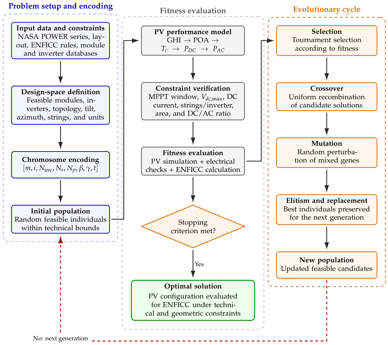
Figure 4.
Graphical analysis of the corrected independent GA runs. Panel (a) compares the final ENFICC of each run with the documented installed baseline and the NASA-based physical-validation value. Panel (b) verifies the equation-level closure between the critical-month energy, the CEN limit, and the final ENFICC. Panel (c) identifies the critical month selected in each run.
Figure 4.
Graphical analysis of the corrected independent GA runs. Panel (a) compares the final ENFICC of each run with the documented installed baseline and the NASA-based physical-validation value. Panel (b) verifies the equation-level closure between the critical-month energy, the CEN limit, and the final ENFICC. Panel (c) identifies the critical month selected in each run.
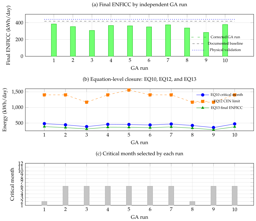
Figure 5.
Normalized equation-level response of the corrected independent GA runs. The heatmap shows that the meteorological equations remain nearly invariant, while the electrical and final-energy equations vary with the design selected by each GA run.
Figure 5.
Normalized equation-level response of the corrected independent GA runs. The heatmap shows that the meteorological equations remain nearly invariant, while the electrical and final-energy equations vary with the design selected by each GA run.
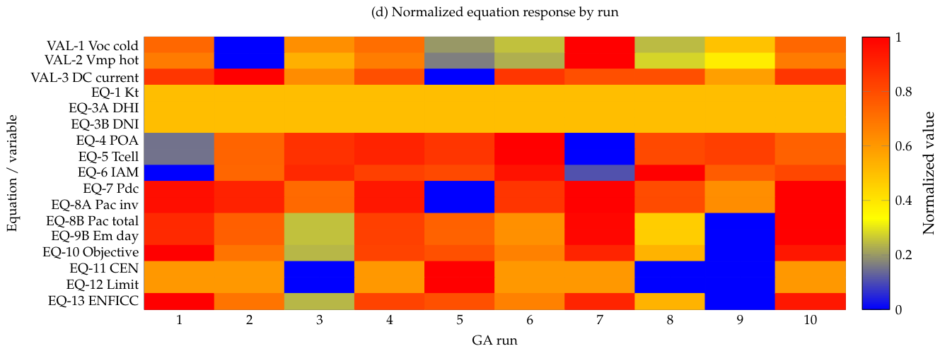
Figure 6.
Coefficient of variation of the main validation and energy equations across the ten corrected independent GA runs. The largest dispersion appears in the DC/AC conversion stage and then propagates to the monthly energy, objective function, and final ENFICC.
Figure 6.
Coefficient of variation of the main validation and energy equations across the ten corrected independent GA runs. The largest dispersion appears in the DC/AC conversion stage and then propagates to the monthly energy, objective function, and final ENFICC.
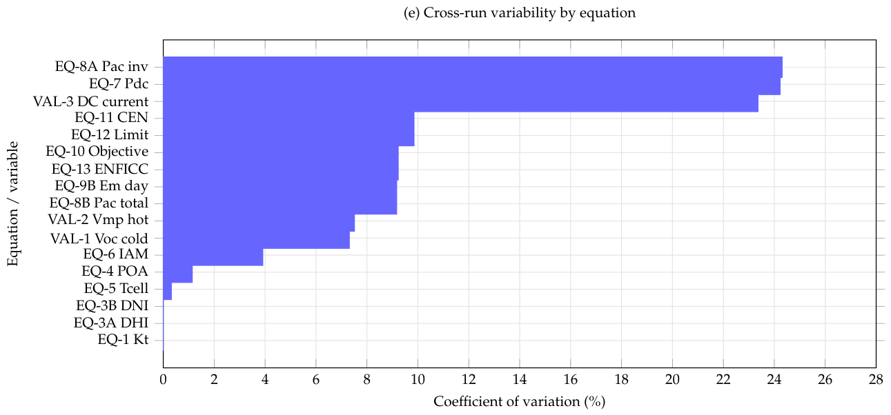

Table 1.
Summary of the La Tebaida validation cases and the best corrected GA run.
| Case | DC | AC | Critical-month energy | Final ENFICC |
|---|---|---|---|---|
| (kWp) | (kW) | (kWh/day) | (kWh/day) | |
| Documented installed baseline | 156.25 | 120 | 520.90 | 416.70 |
| NASA-based physical validation | 157.50 | 120 | 548.50 | 438.80 |
| Best corrected GA run | 135.74 | 120 | 480.20 | 384.16 |
Table 2.
Corrected independent GA runs used for the equation-level graphical analysis.
| Run | DC | AC | Selected module / inverter | Tilt | Azimuth | Critical | Critical | ENFICC |
|---|---|---|---|---|---|---|---|---|
| (kWp) | (kW) | (°) | (°) | month | (kWh/day) | (kWh/day) | ||
| 1 | 135.74 | 120 | LONGi 595M / Solis 60K | 5.75 | 92.48 | 2/2025 | 480.20 | 384.16 |
| 2 | 126.57 | 120 | LONGi 565M / Sungrow 60K | 29.73 | 115.82 | 6/2022 | 441.69 | 353.35 |
| 3 | 109.13 | 100 | LG 410M / SMA 50K | 25.75 | 117.05 | 6/2022 | 384.49 | 307.59 |
| 4 | 128.83 | 120 | LONGi 565M / Solis 60K | 27.21 | 111.39 | 6/2022 | 457.85 | 366.28 |
| 5 | 127.67 | 133 | URE 417M / Siemens 24K | 17.60 | 118.05 | 6/2022 | 453.38 | 362.71 |
| 6 | 121.45 | 120 | LONGi 595M / Canadian 60K | 25.23 | 106.70 | 6/2022 | 437.34 | 349.87 |
| 7 | 139.07 | 120 | Jinko 610M / Huawei 60K | 18.34 | 154.27 | 6/2022 | 468.15 | 374.52 |
| 8 | 117.11 | 100 | Jinko 610M / SMA 50K | 18.80 | 77.12 | 2/2025 | 421.03 | 336.82 |
| 9 | 100.27 | 100 | Solaria 440M / SMA 50K | 28.97 | 111.79 | 6/2022 | 354.37 | 283.50 |
| 10 | 135.74 | 120 | LONGi 595M / Solis 60K | 23.77 | 125.58 | 6/2022 | 472.30 | 377.84 |
Note: The AC column reports the nominal inverter AC capacity used in each GA configuration before applying AC-side and transformer losses in the CEN and energy calculations.
Disclaimer/Publisher’s Note: The statements, opinions and data contained in all publications are solely those of the individual author(s) and contributor(s) and not of MDPI and/or the editor(s). MDPI and/or the editor(s) disclaim responsibility for any injury to people or property resulting from any ideas, methods, instructions or products referred to in the content. |
© 2026 by the authors. Licensee MDPI, Basel, Switzerland. This article is an open access article distributed under the terms and conditions of the Creative Commons Attribution (CC BY) license (http://creativecommons.org/licenses/by/4.0/).
Copyright: This open access article is published under a Creative Commons CC BY 4.0 license, which permit the free download, distribution, and reuse, provided that the author and preprint are cited in any reuse.


