

Submitted:
16 July 2026
Posted:
17 July 2026
You are already at the latest version
Abstract
The flexural behaviour of body-centred cubic (BCC) lattice beams fabricated by stereolithography remains supported by limited experimental evidence, and available homogenized beam models are rarely confronted with data in the combined regime of high relative density, non-slender struts, and low span-to-depth ratios. This work presents an experimental campaign on polymeric BCC lattice beams with three unit-cell edge lengths (L=3, 4, and 5 mm) and a constant strut-to-cell ratio R/L=1/6, yielding a relative density ρ*≈0.423. Specimens were tested under uniaxial compression and three-point bending for nine combinations of geometry. The experimental data are compared with three analytical frameworks: a classical Euler–Bernoulli homogenized beam model and a BCC-specific shear-corrected formulation at the structural level, both evaluated without calibration to the bending tests, together with a strain-gradient extension whose intrinsic length scale is calibrated against them. For the effective Young’s modulus, the closed-form expression of Lee et al. reproduces the compression data within 10%, whereas the Tancogne-Dejean and Mohr model remains markedly stiffer even after the strut-level Timoshenko correction is included. In bending, none of the models proves adequate over the full geometric range: the Euler–Bernoulli model is accurate for several configurations but overestimates the stiffness by up to 108% for the deepest specimen; the shear-corrected model reduces the global root mean square error by approximately a factor of four, but introduces excessive flexibility in some slender and intermediate configurations; and the strain-gradient correction, being strictly stiffening, yields no appreciable improvement. To avoid assigning the discrepancy to a single mechanism, the bending data are further analysed through an experimental compliance decomposition. The additional compliance relative to Euler–Bernoulli theory is small or negative in several cases, showing that shear flexibility alone cannot explain the full dataset, but becomes dominant for the deepest beams. The results therefore delineate the range of validity of simple homogenized beam models for dense finite BCC lattice structures and identify the combined influence of structural shear, non-slender struts, nodal-region morphology, finite-cell and boundary effects, local roller-contact compliance, and the discrete distribution of struts across the cross-section as the main mechanisms requiring more refined descriptions.
Keywords:
BCC lattice
; bending stiffness
; homogenized beam model
; shear correction
; strain-gradient elasticity
; additive manufacturing
1. Introduction
In recent years, advances in additive manufacturing techniques have allowed the development of metamaterials based on lattice structures, which would be unfeasible to obtain using traditional fabrication methods [1,2,3]. Such structures have high potential for industrial applications because their effective mechanical properties can be tailored through the geometry, connectivity, and dimensions of the underlying architecture. Modifications to parameters such as the position, length, and diameter of the bars facilitate the attainment of design-specific properties. This results in architectured materials with favourable strength-to-weight ratios, high energy absorption capacity, and directional stiffness control [4,5]. These characteristics make lattice structures promising candidates as cores of sandwich structures [6,7,8,9], including in aerospace applications [10], where mass reduction and mechanical efficiency are important design drivers [11].
In light of the growing interest in these metamaterials, it is crucial to develop tools that facilitate their design optimization. A substantial body of research has been dedicated to the development of numerical tools for the prediction of the mechanical behaviour of metamaterials based on lattice structures [12,13,14,15]. These models, based on the finite element method, have been demonstrated to accurately predict the behaviour of these metamaterials, with results validated against experimental data.
Although finite element models are an invaluable design tool, the generation of numerical models during the design process can be a laborious and time-consuming process. It is therefore important to develop analytical models that facilitate the design of these metamaterials, not only to optimize the design process but also to enhance comprehension of the fundamental physics underlying these materials.
A substantial body of research has been dedicated to the development of analytical models for the design of metamaterials based on fundamental lattice structures [16,17,18,19]. These models, based on either Euler–Bernoulli beam theory or Timoshenko beam theory, have successfully predicted the tensile and compressive stiffness of blocks composed of these metamaterials, demonstrating a high degree of correlation with experimental results.
As previously stated, one of the principal applications of these metamaterials is as the core of sandwich structures [20,21,22], which are frequently subjected to bending. It is therefore imperative to develop analytical models that can predict the bending stiffness of such structures in a simple and computationally inexpensive manner.
Recently, there has been a growing interest in developing analytical models to predict the bending stiffness of lattice metamaterials based on octet-truss structures. In the work presented by Korshunova et al. [23], a variety of models were introduced based on classical beam theory and strain-gradient theory. The capability of these models was then validated with experimental and numerical results. However, in their work, the application of the analytical models entailed the introduction of an equivalent elastic modulus, which was defined based on experimental or numerical results.
To address these issues, the objective of this study is not only to compare analytical predictions against bending experiments, but also to identify which parts of the discrepancy can and cannot be interpreted within simple homogenized beam descriptions. This distinction is important for dense finite lattices, for which the specimen may behave partly as an architectured material with effective properties and partly as a discrete structure governed by finite-cell geometry, boundary cells, nodal regions, and contact conditions. The bending rigidity is first predicted by combining an effective Young’s modulus obtained from unit-cell analytical models with a homogenized Euler–Bernoulli beam formulation. A shear-corrected homogenized beam model is then evaluated to represent the additional flexibility expected in deep beams with low span-to-depth ratios. Finally, a strain-gradient extension is considered as an additional correction introducing an intrinsic length scale parameter to account for possible size-dependent stiffening effects. To validate and critically assess these descriptions, experiments were conducted on resin specimens manufactured using low-force stereolithography, with three different unit-cell sizes considered. The experimental campaign includes both uniaxial compression tests of the resin material and the BCC structures, used to assess the accuracy of the effective Young’s modulus predictions, and three-point bending tests of the BCC structures, which constitute the primary validation dataset for the bending rigidity models. In addition to the direct stiffness comparison, an experimental compliance decomposition is introduced to quantify the apparent non-Euler–Bernoulli contribution without requiring additional numerical simulations.
2. Experimental Setup
2.1. Geometry and Material Characterization
The specimens employed in this study were produced using low-force stereolithography (LFS), with a Raise3D DF2 resin 3D printer and Apricot V1 resin supplied by Raise3D. The printing parameters—such as layer thickness, fixed at 0.05 mm, build orientation, and support structures—were carefully selected to ensure dimensional accuracy and adequate mechanical performance. After fabrication, all specimens were post-cured using a DF-Cure system, with each side exposed for 15 minutes under ambient conditions.
In order to characterize the mechanical properties of the base material, uniaxial compression tests were performed on solid cylindrical specimens with a height of 30 mm and a diameter of 10 mm. The tests were conducted using a servo-hydraulic universal testing machine (Instron 8801) with a 150 kN frame, at a constant displacement rate of 1 mm/min. The load was applied to the specimens via 150 kN rated compression plates, thus minimizing the effect of machine compliance on the results. Load and displacement data were extracted from the 100 kN load cell and the LVDT equipped with the machine. Both the specimen geometry and testing conditions were defined in accordance with ASTM D695.
A total of three tests were carried out for the characterization of the resin’s elastic properties, and a representative stress–strain curve is presented in Fig. Figure 1. Based on these experiments, the Young’s modulus of the material was determined as . The measured density of the resin was , in agreement with the manufacturer’s specifications.
Figure 1.
Representative stress–strain curve obtained from the compression tests on cylindrical resin specimens.
Figure 1.
Representative stress–strain curve obtained from the compression tests on cylindrical resin specimens.
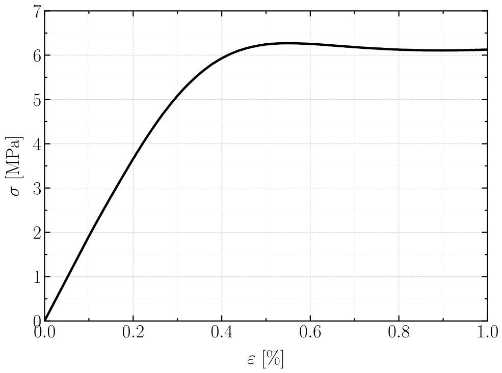
Figure 2.
Configuration of the BCC unit cell.
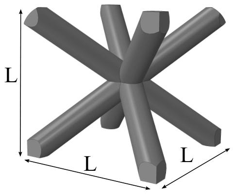
For specimens made of a single material with uniform circular struts of radius R, it is necessary to distinguish between the cubic unit-cell edge length, denoted here as L, and the center-to-vertex strut length, denoted as ℓ. For a BCC unit cell,
Following the geometrical convention used by Tancogne-Dejean and Mohr [24], the relative density of a BCC lattice made of uniform circular struts is expressed in terms of as
This expression accounts for the volume of the struts and the nodal intersections. The beam intersections are referred to as nodes, whose volume fraction becomes increasingly important as the relative density increases. For example, Tancogne-Dejean and Mohr report that approximately 5% of the solid phase is contained in the nodes at , whereas the nodal contribution increases to approximately 40% at . Therefore, the present relative density, , places the specimens in a regime where the nodal regions and the non-slender character of the struts cannot be regarded as small perturbations. This point is retained throughout the discussion: the analytical strut-based expressions are used as compact homogenized estimates, but the observed bending response may also be affected by nodal morphology, finite-cell cross-sections, and boundary-cell effects.
Three cubic unit-cell edge lengths were considered, , 4, and 5 mm. Rather than fixing the strut radius, the ratio between the strut radius and the unit-cell edge length was kept constant at
This resulted in nominal strut radii of , 0.667, and 0.833 mm for , 4, and 5 mm, respectively. Using Eq. (1), these values correspond to
Substituting into Eq. (2) gives an approximately constant relative density of for all configurations.
2.2. Compression Tests
Uniaxial compression tests were performed on cubic lattice specimens to evaluate their effective mechanical response. Each specimen was designed with six unit cells along each spatial direction, resulting in overall dimensions of 18 mm, 24 mm and 30 mm for unit cell edge lengths of , 4 and 5 mm, respectively, as shown in Fig. Figure 3.
The tests were conducted using the same testing machine and testing conditions as previously described for material characterization, under displacement control at a constant loading rate of 1 mm/min. For each configuration, three tests were performed to ensure repeatability.
From the obtained force–displacement curves, the initial stiffness of each specimen was determined. A representative force–displacement curve for each test sample size is presented in Fig. Figure 4. As can be observed, both the maximum load and the initial stiffness increase as the unit cell size increases, while maintaining a constant number of unit cells. These results provide a qualitative comparison of the mechanical response, whereas the corresponding quantitative values are discussed in conjunction with the analytical predictions in the Results section.
2.3. Bending Tests
The beams were subjected to three-point bending tests with a support span of mm throughout the experiments, as shown in Fig. Figure 5. The overall beam length was kept constant at 100 mm in all cases. The radius of the loading and support rollers was mm.
The lattice architecture was defined by limiting the number of unit cells across the beam width to four unit cells. The beam height was varied considering 4, 6, and 8 unit cells in the vertical direction, allowing the influence of the structural height h to be investigated while maintaining a constant beam length. The experiments were carried out with the same test machine previously described, although the load cell was swapped by a 5 kN cell to increase the precision of the results. Each specimen was tested a minimum of three times at a speed of 1 mm/min under ambient laboratory conditions of 20–25 °C.
The vertical displacement u at the loading point was recorded directly from the crosshead of the testing machine. Two factors support the use of this measurement as an estimate of the mid-span deflection of the specimens. First, the bending loads involved were modest (of the order of tens to a few hundred newtons) and were applied through a stiff servo-hydraulic frame equipped with a 5 kN load cell, so that the elastic compliance of the machine is expected to be small compared with the deflection of the beams. Second, despite their cellular nature, the specimens are comparatively stiff owing to their high relative density (), and the loading and support rollers, of radius mm, distribute the contact force over several surface struts. Nevertheless, local contact compliance at the roller–lattice interface cannot be ruled out from the present measurements and is therefore considered as one of the possible contributors to the apparent additional compliance discussed below.
Representative force–displacement curves obtained from the three-point bending tests are presented in Fig. Figure 6 for unit-cell edge lengths , 4, and 5 mm. In each case, results are shown for beam heights corresponding to 4, 6, and 8 unit cells in the vertical direction. As expected, an increase in beam height h leads to a notable increase in both the initial stiffness and the failure load. Conversely, the displacement at failure decreases with increasing h, which is consistent with the higher stress concentrations induced in stiffer configurations. Failure occurred in a brittle manner in all tested configurations: upon reaching the maximum load, a sudden and abrupt drop in the recorded force was observed, with no evidence of a progressive or ductile post-peak response. In every specimen, fracture initiated at mid-span on the lower (tensile) face of the beam and propagated upwards through the lattice. This consistent failure location indicates that tensile stresses on the bottom fibers govern the ultimate response, which is also in line with the brittle nature of the photopolymer resin and justifies the abrupt load drop observed across all unit-cell sizes and beam heights considered in this study.
3. Analytical Models
In this section, the analytical models employed to predict the mechanical behavior of the BCC lattice structures are presented. First, two expressions for the effective Young’s modulus are introduced. The model of Tancogne-Dejean and Mohr [24] is formulated in terms of the closest-neighbor distance ℓ, whereas the expression of Lee et al. [25] is evaluated using the cubic unit-cell dimensions. The distinction between L and ℓ is therefore retained throughout the analysis. Subsequently, the bending rigidity of the homogenized beam is derived using a classical Euler–Bernoulli beam model, a BCC-specific shear-corrected homogenized beam model, and a strain-gradient Euler–Bernoulli extension. The shear-corrected model uses an analytical BCC shear modulus at the unit-cell level and introduces a finite-section shear-efficiency factor to account for the discrete shear-transfer mechanism of the lattice beam.
3.1. Effective Young’s Modulus
3.1.1. Model Based on Tancogne-Dejean and Mohr (2018)
Tancogne-Dejean and Mohr [24] derived closed-form expressions for the homogenized elastic moduli of BCC truss lattices. In their formulation, the characteristic length ℓ corresponds to the closest-neighbor distance. Therefore, the relevant geometrical parameter for this model is
For beams of uniform circular cross-section and negligible shear deformation at the strut level, the Euler–Bernoulli expression for the Young’s modulus in the direction can be written as
Because the present struts are relatively stocky, the Timoshenko-corrected version of the model was also evaluated following the stiffness-based formulation given by Tancogne-Dejean and Mohr. The details of this calculation, including the evaluation of , , the nodal correction factor , and the Timoshenko correction factor , are provided in Appendix A.
3.1.2. Model Based on Lee et al. (2019)
An alternative expression for the effective Young’s modulus of BCC lattice structures was proposed by Lee et al. [25], based on a free-body diagram analysis of the BCC unit cell subjected to compressive loading. The displacement of the unit cell is decomposed into axial and bending contributions of the individual struts following Euler–Bernoulli beam theory. For a cubic unit cell with L and circular cross-section of radius R, the effective Young’s modulus reads
Unlike the model of Tancogne-Dejean and Mohr, this expression is based on a direct free-body analysis of the cubic BCC unit cell and does not explicitly introduce a nodal-volume correction. In the present work, it is retained as a compact analytical estimate directly expressed in terms of the cubic unit-cell dimensions.
It is worth noting that the analytical approach adopted by Lee et al. [25] is based on the methodology originally proposed by Ptochos and Labeas [26], who derived closed-form expressions for the effective elastic modulus of BCC micro-lattice structures by decomposing the strut deformation into axial and bending contributions within the framework of Euler–Bernoulli beam theory. The model of Lee et al. follows the same theoretical foundation and, for the cubic unit-cell case considered in the present work, yields predictions that differ only marginally from those of Ptochos and Labeas. For this reason, only the expression proposed by Lee et al. is retained in the following bending comparisons, as it provides a compact closed-form expression directly applicable to the BCC unit-cell geometry considered here.
3.2. Bending Rigidity
3.2.1. Classical Euler–Bernoulli Beam Model
The classical Euler–Bernoulli solution gives the maximum mid-span deflection under three-point bending as
where is the support span, P is the applied load, is the effective Young’s modulus, and is the homogenized second moment of area. The latter is approximated using the outer dimensions of the lattice beam as
where b is the width and h is the height of the homogenized rectangular cross-section. The corresponding homogenized cross-sectional area is
The cross-sectional dimensions and the corresponding values of and for each specimen configuration are listed in Table 1.
The bending stiffness, defined as , can then be written as
3.2.2. Shear-Corrected Homogenized Beam Model
The classical Euler–Bernoulli formulation assumes that the transverse deflection is dominated by bending and neglects shear deformation. This approximation is appropriate for slender beams, but it may become inaccurate when the span-to-depth ratio decreases. In the present experimental campaign, the support span was kept constant at , whereas the beam height varied from to . Therefore, the ratio ranges from 6.67 for the most slender configuration to 2.00 for the deepest beam. For the latter configurations, shear flexibility at the structural beam level may contribute significantly to the measured displacement.
To account for this effect, a shear-corrected homogenized beam model is introduced. The total mid-span deflection under three-point bending is written as the sum of a bending contribution and a shear contribution,
where is the effective Young’s modulus of the BCC lattice, and are the gross second moment of area and cross-sectional area of the homogenized beam, is the effective shear modulus of the BCC unit cell, and is a finite-section shear-efficiency factor for the BCC lattice beam.
The corresponding initial stiffness is
Equivalently,
with
This form shows explicitly that the shear correction becomes relevant as increases. For slender beams, , and therefore , recovering the Euler–Bernoulli prediction. For deeper beams, , and the effective stiffness is reduced by the additional shear compliance.
The classical value is the shear correction factor commonly associated with a homogeneous rectangular section, obtained from an energy-equivalent representation of the non-uniform shear stress distribution. A BCC lattice beam, however, is not a homogeneous solid rectangular section. Its shear response is governed by a finite number of inclined struts, discrete nodal regions, non-periodic boundary conditions, and local perturbations introduced by the loading and support rollers. Therefore, the rectangular-section value is not adopted directly as the final shear correction factor.
The effective shear modulus of the BCC unit cell is instead estimated from the analytical expression proposed for regular BCC open-cell structures by Ptochos and Labeas,
For the present geometry, with and , this gives
This value should be interpreted as a unit-cell-level homogenized shear modulus over the gross cell volume.
Since the finite lattice beam does not transmit shear through a continuous rectangular solid area, an additional section-efficiency factor is introduced. As a first-order approximation, this factor is taken as
The factor accounts for the fact that only a fraction of the gross cross-section is occupied by solid material, while the factor provides a simple orientation-efficiency estimate associated with the three-dimensional inclined strut network. For the present specimens, , and therefore
It is important to emphasize that Eq. (18) is not introduced as an independently validated material parameter. Rather, it is used as a compact engineering estimate of the apparent shear-transfer efficiency of a finite BCC lattice section. It collects, in an average sense, the fact that the section is discrete, that shear is transmitted through a finite number of inclined struts and nodal regions, and that boundary cells and roller-contact perturbations may alter the local deformation field. The shear-corrected model is therefore interpreted as a diagnostic homogenized description of the additional compliance expected in deep beams, not as a universal predictive theory for all lattice geometries.
3.2.3. Strain-Gradient Euler–Bernoulli Beam Model
In the scope of the present work, we also consider the strain-gradient beam theory presented in [23,27,28]. The deflection for the Euler–Bernoulli beam within the strain-gradient framework is given by
where g is the intrinsic length scale parameter, which acts as a higher-order material parameter depending on the microstructure of the unit cell. This parameter characterises size-dependent beam behaviour, in which smaller beams may exhibit a stiffening effect relative to the prediction of classical theory. The corresponding bending stiffness reads
The additional term reflects the contribution of the microstructural length scale to the overall bending resistance and directly implies that for any nonzero value of g. Consequently, the strain-gradient formulation consistently predicts higher bending stiffnesses than the classical theory, with the difference becoming more pronounced as the beam height h decreases relative to g.
It should therefore be noted that this correction can only increase the stiffness predicted by the classical Euler–Bernoulli model. Consequently, it cannot improve configurations for which the classical model already overestimates the experimental stiffness. In the present work, g is calibrated from the bending data for each unit-cell edge length in order to assess whether such a correction can improve the predictions. However, the resulting values and their effect on the model accuracy are discussed critically in the Results section.
4. Results and Discussion
This section presents a comprehensive comparison of the experimental and analytical results obtained for the BCC lattice specimens considered in this study. The analysis is organized into two parts: uniaxial compression results and three-point bending results. For each case, the predictions derived from the analytical models are contrasted against the experimentally measured data. The predictive capability of each model is evaluated in terms of initial stiffness. Special attention is given to the influence of the unit cell edge length L, the beam height h, and the span-to-depth ratio on the mechanical response, as well as to the limitations of each modelling approach in capturing the observed behaviour.
4.1. Compression Results
The mean values and standard deviations of the effective Young’s modulus obtained from the three compression tests performed for each unit-cell size are presented in Table 2, together with the analytical predictions derived from the models of Tancogne-Dejean and Mohr [24] and Lee et al. [25]. The standard deviation values are in all cases below 10% of the mean, which is considered a reasonable level of dispersion for this type of experimental campaign and demonstrates the good repeatability of the results.
As can be observed, the model of Lee et al. provides predictions in close agreement with the experimental results, with discrepancies below approximately 10% for all unit-cell sizes. In contrast, the Euler–Bernoulli version of the Tancogne-Dejean and Mohr model significantly overestimates the effective Young’s modulus. When the Timoshenko correction at the strut level is included, the prediction is reduced from MPa to MPa. Although this correction substantially improves the prediction, the model still remains stiffer than the experimental response. This discrepancy may be associated with the assumptions of ideal periodicity, rigid nodes, affine nodal motion, and perfect strut geometry, which are particularly strong for additively manufactured polymeric specimens.
Regarding maximum compressive stress, the mean values obtained experimentally are MPa, MPa, and MPa for unit-cell edge lengths , 4, and 5 mm, respectively. A slight decrease in failure stress is observed with an increase in unit-cell size, which is consistent with the trend observed for the effective Young’s modulus and reflects the influence of the structural scale on the failure behavior of the lattice specimens.
As shown in this section, the model proposed by Lee et al. [25] provides excellent agreement with the experimental results in terms of effective Young’s modulus prediction. For this reason, the bending stiffness predictions presented in the following section adopt the effective modulus obtained from the model of Lee et al., Eq. (7), as input to the homogenized beam models.
4.2. Bending Results
The mean values of initial stiffness obtained from the three-point bending tests are presented in Table 3, together with the corresponding standard deviations, the predictions of the classical Euler–Bernoulli model, and those of the BCC shear-corrected homogenized beam model evaluated using Eqs. (13)–(19). As expected, the initial stiffness increases monotonically with beam height h for all unit-cell sizes considered. The standard deviation values are generally small relative to the mean, indicating good repeatability across the three tests performed for each configuration. The comparison between measured and predicted stiffness is summarized graphically in Fig. Figure 7, in which departures from the dashed diagonal directly indicate prediction errors.
The results show that the classical Euler–Bernoulli model provides predictions of acceptable accuracy for several configurations considered, with errors below approximately 16% in five out of nine cases. However, significant discrepancies are observed in specific configurations. The largest errors occur for mm with the shortest beam ( mm, error of 24.0%), for mm with the tallest beam ( mm, error of 34.4%), and for mm with the tallest beam ( mm, error of 108.3%). It is also worth noting that the classical model does not exhibit a consistent bias: in some configurations it underestimates the experimental stiffness, while in others it overestimates it, as is apparent from the distribution of points on both sides of the diagonal in Fig. Figure 7. This suggests that the discrepancies are not solely attributable to a systematic limitation of the homogenization approach, but rather to the combined influence of shear flexibility, boundary effects, discrete lattice architecture, and the ratio between the beam height and the span length.
The BCC shear correction has a minor effect for the most slender specimens, but becomes increasingly relevant as the span-to-depth ratio decreases. As shown in Table 3 and Fig. Figure 7, the correction substantially reduces the overprediction for the deepest beams, at the cost of introducing additional flexibility in configurations for which the Euler–Bernoulli prediction was already accurate.
4.2.1. Experimental Compliance Decomposition
To avoid attributing all discrepancies to a single mechanism, the bending data were further analyzed in terms of compliance rather than stiffness. The experimental and Euler–Bernoulli compliances are defined as
and the apparent non-Euler–Bernoulli contribution is written as
A normalized measure of this additional compliance is therefore
This quantity is useful because shear deformation, contact compliance, and local deformation mechanisms can only add compliance to the Euler–Bernoulli bending contribution. Therefore, configurations with are more compliant than predicted by the classical homogenized beam model, whereas configurations with are experimentally stiffer than the Euler–Bernoulli prediction and cannot be explained by shear flexibility alone.

Table 4.
Experimental compliance decomposition relative to the Euler–Bernoulli prediction. The apparent efficiency factor is reported only for configurations with and should be interpreted as an apparent shear/contact/finite-size efficiency, not as an independently measured shear correction factor.
Table 4.
Experimental compliance decomposition relative to the Euler–Bernoulli prediction. The apparent efficiency factor is reported only for configurations with and should be interpreted as an apparent shear/contact/finite-size efficiency, not as an independently measured shear correction factor.
| L | h | |||
|---|---|---|---|---|
| [mm] | [mm] | [-] | [-] | [-] |
| 12.0 | 6.67 | -0.239 | – | |
| 3.0 | 18.0 | 4.44 | -0.033 | – |
| 24.0 | 3.33 | 0.019 | 2.17 | |
| 16.0 | 5.00 | 0.041 | 0.44 | |
| 4.0 | 24.0 | 3.33 | 0.116 | 0.35 |
| 32.0 | 2.50 | 0.344 | 0.21 | |
| 20.0 | 4.00 | -0.254 | – | |
| 5.0 | 30.0 | 2.67 | 0.153 | 0.41 |
| 40.0 | 2.00 | 1.083 | 0.10 |
For the configurations with , an apparent efficiency factor can be obtained by equating the measured additional compliance to a Timoshenko-like shear term,
which gives
The resulting values vary substantially across the tested geometries, from values above unity when the additional compliance is nearly negligible to approximately for the deepest beam. This confirms that a single constant shear-efficiency factor cannot be interpreted as a universal property of the lattice material. Instead, should be understood as an apparent parameter that collects structural shear, local contact compliance, finite-cell effects, nodal-region deformation, and the discrete distribution of load paths across the section.
The BCC shear-corrected model substantially reduces the overprediction observed for the deepest beams. The most notable case is the configuration , , for which the Euler–Bernoulli model predicts an initial stiffness of , whereas the experimental value is . Including the BCC shear correction reduces the prediction to , decreasing the error from to . A similar improvement is observed for , , where the error decreases from to .
However, the shear correction does not improve all configurations. For the series, the Euler–Bernoulli model already provides accurate predictions for and . In these cases, the additional shear flexibility introduced by the BCC correction leads to an underestimation of the experimental stiffness. The compliance decomposition clarifies this behavior: several slender or intermediate configurations have or even , meaning that there is little apparent additional compliance to be corrected, or that the experiment is stiffer than the Euler–Bernoulli estimate. Such cases cannot be explained by structural shear alone. They likely reflect the combined influence of discrete cross-sectional architecture, finite-cell geometry, nodal-region morphology, and the fact that the gross-section inertia used in the homogenized beam model is only an idealized representation of the actual lattice section.
Overall, the comparison suggests that Euler–Bernoulli theory is adequate for the configurations in which the apparent additional compliance remains small, whereas the BCC shear-corrected model becomes more appropriate for the deepest beams with low ratios. Therefore, the two models should not be interpreted as competing universal descriptions. The complementary character of the two formulations can be described through a single dimensionless parameter. From Eq. (12), the ratio of the shear to the bending compliance is
which is precisely the term entering in Eq. (15). Shear flexibility ceases to be a minor perturbation once it contributes a comparable fraction of the total compliance; adopting as a practical diagnostic threshold, the BCC shear-corrected model is preferable for and the classical Euler–Bernoulli model otherwise. For the present lattice, , so this threshold corresponds to . This criterion identifies precisely the deep configurations for which the shear-corrected model gives the lower prediction error ( and ). The threshold should be regarded as indicative, since it was established from nine configurations at a single relative density and strut-to-cell ratio; its transferable form is the compliance ratio rather than the bare span-to-depth ratio.
4.2.2. Role of Non-Slender Struts, Nodes, and Finite-Cell Effects
The compliance analysis also shows why the observed discrepancies should not be assigned exclusively to shear deformation. The present specimens have and , so the struts are not slender in the asymptotic sense assumed by many truss-based homogenized expressions, and the nodal regions represent a non-negligible fraction of the solid phase. Under bending, these nodal regions are not merely passive volume corrections: they affect the rotational stiffness of strut junctions, the transfer of shear across the section, and the way boundary cells interact with the loading and support rollers.
Moreover, the beam cross-section contains only four unit cells across the width and four to eight unit cells through the height. The use of the gross rectangular second moment of area in Eq. (9) is therefore a homogenized approximation to a strongly discrete distribution of load-bearing struts. Depending on the relative position of the outer struts, boundary nodes, and roller contact regions, this approximation may either overestimate or underestimate the actual bending stiffness. This explains why the sign of is not uniform across the dataset. Positive values of indicate missing compliance relative to the Euler–Bernoulli model, whereas negative values indicate that the experimental structure is stiffer than the gross-section homogenized estimate. The latter cases cannot be corrected by adding a Timoshenko-like shear term, because such a term only increases compliance.
Consequently, the shear-corrected model is best interpreted as a low-order representation of the deep-beam regime rather than as a complete physical decomposition. The present experiments support the conclusion that deep dense BCC lattice beams require additional non-Euler–Bernoulli compliance, but the data alone do not uniquely separate structural shear from nodal deformation, contact compliance, and finite-cell effects.
The initial stiffness predictions obtained from the Euler–Bernoulli, strain-gradient Euler–Bernoulli, and shear-corrected homogenized beam models are compared against the experimental results in Fig. Figure 8. For the strain-gradient model, the intrinsic length scale parameter g was determined for each unit-cell edge length by minimizing the root mean square error with respect to the experimental data. The calibrated values obtained are mm for mm, and mm for both mm and mm. The latter result implies that the strain-gradient correction vanishes for the two larger unit-cell sizes, and both models therefore yield identical predictions in those cases.
The intrinsic length parameter g was calibrated independently for each unit-cell edge length. For mm, the calibrated value mm produces only a minor modification of the classical Euler–Bernoulli prediction, because g remains much smaller than the beam heights considered. The maximum correction occurs for mm and is approximately 2.6%. For and 5 mm, the optimal value is , and the strain-gradient model therefore collapses to the classical Euler–Bernoulli prediction. This result is expected because the adopted strain-gradient correction is strictly stiffening, whereas the largest discrepancies occur in configurations for which the classical model already overestimates the experimental stiffness. This confirms that the strain-gradient correction does not provide a significant improvement for the present dataset.
Table 5 presents the root mean square error (RMSE) of the initial stiffness predictions obtained from the Euler–Bernoulli, strain-gradient Euler–Bernoulli, and shear-corrected homogenized beam models.
The RMSE values confirm that the strain-gradient correction does not significantly modify the Euler–Bernoulli predictions for the present dataset. In contrast, the BCC shear-corrected model substantially reduces the global RMSE, from to . This improvement is mainly associated with the deepest beams, for which the span-to-depth ratio is low and the compliance decomposition indicates a large positive . Nevertheless, the model worsens the predictions for , where the Euler–Bernoulli approximation was already accurate or slightly conservative. This behavior reinforces the regime-dependent interpretation: Euler–Bernoulli theory is more suitable when the apparent additional compliance is small, whereas the BCC shear-corrected formulation is more appropriate as a diagnostic approximation for deep lattice beams in which becomes significant.
The maximum loads recorded during the three-point bending tests are presented in Table 6. As observed for the initial stiffness, the maximum load increases monotonically with beam height h for all unit-cell sizes. The standard deviation values are in most cases below 15% of the mean, reflecting acceptable repeatability, with the exception of the configuration mm, mm, which exhibits a somewhat larger dispersion likely associated with the inherent variability of the failure process in brittle lattice structures.
For a fixed unit-cell size, the maximum load scales strongly with beam height, which is consistent with the increased cross-sectional resistance of taller specimens. Comparing across unit-cell sizes at equivalent beam heights, larger unit cells tend to sustain higher failure loads, which can be attributed to the greater strut radius used in those configurations to maintain a constant . As discussed previously, failure occurs in a brittle manner in all cases, with an abrupt load drop upon reaching , and no evidence of progressive post-peak response.
It is worth noting that, given the brittle failure observed in all configurations and the absence of a progressive post-peak response, the energy absorbed up to peak load is essentially governed by the initial stiffness and the displacement at failure. Consequently, integrating the force–displacement curves does not provide additional physical insight beyond the initial stiffness and maximum load values already reported in Table 3 and Table 6.
5. Conclusions
This work presented a combined experimental and analytical study of the flexural behaviour of polymeric BCC lattice beams fabricated by low-force stereolithography. Nine beam configurations, spanning three unit-cell edge lengths ( mm) at a constant strut-to-cell ratio (), were tested under three-point bending, with the effective Young’s modulus independently characterized by uniaxial compression on cubic specimens. Three homogenized frameworks were assessed: a classical Euler–Bernoulli model and a BCC shear-corrected model, both evaluated without calibration to the bending data, and a strain-gradient extension whose intrinsic length scale was calibrated against them.
For the effective modulus, the closed-form expression of Lee et al. [25] reproduced the compression data within approximately 10%, whereas the Tancogne-Dejean and Mohr model [24] remained markedly stiffer even after the strut-level Timoshenko correction. The former was therefore adopted as input to the bending models. This agreement should nevertheless be interpreted with caution: strut-based analytical models are nominally restricted to idealized slender-strut lattices, whereas the present specimens lie in a dense regime in which nodal regions and non-slender struts are expected to influence the mechanical response.
In bending, no single homogenized model proved adequate over the full geometric range. The Euler–Bernoulli formulation performed well for several configurations but overestimated the stiffness by more than 100% for the deepest specimen. The shear-corrected model, based on the BCC unit-cell shear modulus and the first-order finite-section efficiency estimate , brought the deep-beam predictions within approximately 16% and reduced the global RMSE from to . However, it introduced excessive flexibility in configurations for which the Euler–Bernoulli model was already accurate. The shear-corrected formulation should therefore not be interpreted as a universal predictive theory, but as a low-order diagnostic correction for the deep-beam regime.
A compliance decomposition was introduced to make this interpretation explicit. The normalized additional compliance was close to zero or negative in several slender and intermediate configurations, showing that the discrepancy cannot be attributed to shear flexibility alone. In contrast, increased strongly for the deepest beams, reaching for and , meaning that the experimental compliance was more than twice the Euler–Bernoulli bending compliance. An apparent efficiency factor was also extracted for the cases with positive additional compliance. Its strong variation across the dataset confirms that the apparent extra compliance collects several mechanisms, including structural shear, local roller-contact compliance, finite-cell effects, nodal-region deformation, and the discrete distribution of struts across the section.
The two beam descriptions are therefore complementary rather than competing. Their range of applicability can be described through the shear-to-bending compliance ratio : the shear-corrected model is preferable for and the Euler–Bernoulli model otherwise, a threshold that for the present lattice corresponds to . This criterion should be regarded as indicative, since it was established from nine configurations at a single relative density and strut-to-cell ratio. The strain-gradient extension yielded no appreciable improvement: being strictly stiffening, it cannot recover configurations in which the classical model already overpredicts the response.
Taken together, these findings delineate the range of validity of simple homogenized beam models for dense finite BCC lattice structures. The main conclusion is not that a single missing correction explains the experiments, but rather that the flexural response results from the combined influence of structural shear, non-slender struts, nodal-region morphology, finite-cell and boundary effects, local roller-contact compliance, and the discrete cross-sectional distribution of struts. The dataset and compliance-based interpretation reported here are intended to support the development and validation of more refined descriptions, such as discrete-section or micro-polar lattice beam formulations, together with independent future measurements or simulations of shear and contact effects.
Author Contributions
Conceptualization, G.S.-A. and M.B.; methodology, G.S.-A., M.M.M.C., J.P. and M.B.; software, G.S.-A.; validation, G.S.-A., M.M.M.C. and J.P.; formal analysis, G.S.-A. and M.B.; investigation, G.S.-A.; writing—original draft preparation, G.S.-A.; writing—review and editing, M.M.M.C., J.P. and M.B.; supervision, M.B. All authors have read and agreed to the published version of the manuscript.
Funding
This research received no external funding.
Institutional Review Board Statement
Not applicable.
Informed Consent Statement
Not applicable.
Data Availability Statement
The data presented in this study are available on request from the corresponding author.
Acknowledgments
Not applicable.
Conflicts of Interest
The authors declare no conflicts of interest.
Appendix A. Details of the Analytical Evaluation of the Effective Young’s Modulus
This appendix summarizes the analytical calculations used to evaluate the effective Young’s modulus of the BCC lattice specimens. Two models are considered: the expression proposed by Lee et al. [25], and the stiffness-based formulation of Tancogne-Dejean and Mohr [24]. Particular attention is paid to the distinction between the cubic unit-cell edge length and the closest-neighbor distance, since this distinction affects the evaluation of both the relative density and the Tancogne-Dejean and Mohr model.
Appendix A.1. Geometrical Definitions
The specimens considered in this work are based on a cubic BCC unit cell of edge length L. The struts connect the center of the cube to its eight vertices. Therefore, the center-to-vertex distance, also referred to as the closest-neighbor distance, is
In the present specimens, the strut radius was scaled with the unit-cell edge length, such that
The geometrical values used in the calculations are summarized in Table A1.
Table A1.
Geometrical parameters used for the analytical evaluation of the BCC lattice specimens. Here, L denotes the cubic unit-cell edge length and ℓ denotes the center-to-vertex strut length.
Table A1.
Geometrical parameters used for the analytical evaluation of the BCC lattice specimens. Here, L denotes the cubic unit-cell edge length and ℓ denotes the center-to-vertex strut length.
| L | R | ℓ | ||
|---|---|---|---|---|
| [mm] | [mm] | [mm] | [-] | [-] |
| 3.0 | 0.500 | 2.598 | 0.1667 | 0.1925 |
| 4.0 | 0.667 | 3.464 | 0.1667 | 0.1925 |
| 5.0 | 0.833 | 4.330 | 0.1667 | 0.1925 |
It is useful to emphasize the geometrical convention adopted in the present work. Here, L denotes the edge length of the cubic BCC unit cell, consistently with the notation used in the specimen drawings and experimental description. The center-to-vertex distance, or closest-neighbor distance, is denoted by ℓ. The analytical formulation of Tancogne-Dejean and Mohr is evaluated in terms of this closest-neighbor distance. Therefore, when their model is applied to the present specimens, the relevant geometrical parameter is not , but
For the present geometry, , and therefore
On the other hand, the model of Lee et al. is directly expressed in terms of the cubic unit-cell dimensions. Consequently, the relevant geometrical parameter for that model is
This distinction is retained throughout the calculations below.
Appendix A.2. Relative Density
For a BCC lattice made of uniform circular struts, Tancogne-Dejean and Mohr [24] express the relative density as
Using , this can be written as
For and , for example,
and therefore
The resulting relative density is the same for the three unit-cell sizes because was kept constant. The values are shown in Table A2.
Table A2.
Relative density obtained using the geometrical convention of Tancogne-Dejean and Mohr [24].
Table A2.
Relative density obtained using the geometrical convention of Tancogne-Dejean and Mohr [24].
| L | ||
|---|---|---|
| [mm] | [-] | [-] |
| 3.0 | 0.1925 | 0.423 |
| 4.0 | 0.1925 | 0.423 |
| 5.0 | 0.1925 | 0.423 |
Appendix A.3. Effective Young’s Modulus According to Lee et al. (2019)
Lee et al. [25] derived an analytical expression for the effective Young’s modulus of a BCC lattice under compressive loading by decomposing the strut displacement into axial and bending contributions. For the cubic case considered here, the expression can be written as
where
and is the Young’s modulus of the base material. In this work,
Since for all configurations,
Substituting into Eq. (A11),
The values obtained for all specimens are summarized in Table A3.
Table A3.
Effective Young’s modulus predicted by the model of Lee et al. [25].
Table A3.
Effective Young’s modulus predicted by the model of Lee et al. [25].
| L | R | ||
|---|---|---|---|
| [mm] | [mm] | [-] | [MPa] |
| 3.0 | 0.500 | 0.1667 | 54.88 |
| 4.0 | 0.667 | 0.1667 | 54.88 |
| 5.0 | 0.833 | 0.1667 | 54.88 |
Since is constant for the three configurations, Eq. (A11) predicts the same effective Young’s modulus, , for all unit-cell sizes. This value is adopted in the bending calculations reported in the main text.
Appendix A.4. Effective Young’s Modulus According to Tancogne-Dejean and Mohr
The model of Tancogne-Dejean and Mohr [24] is formulated in terms of the axial stiffness and the effective flexural stiffness of a doubly-clamped beam embedded in the BCC network. The effective Young’s modulus in the direction can be written as
In this formulation, the free length of the deformable part of the strut is reduced by the presence of rigid nodal regions. This is accounted for through
with
For uniform circular struts, the axial stiffness is
The Euler–Bernoulli flexural stiffness is
For relatively stocky beams, Tancogne-Dejean and Mohr also introduce a Timoshenko correction through the factor , such that
where
The Poisson’s ratio of the base material is taken as
For , , and , the nodal correction factor is
The axial stiffness is therefore
The Euler–Bernoulli flexural stiffness is
Thus,
Substitution into Eq. (A16) gives
For the Timoshenko correction, the shear correction factor is
Therefore,
and
The Timoshenko-corrected effective Young’s modulus is then
The complete set of values is given in Table A4.
Table A4.
Intermediate quantities and effective Young’s modulus predicted by the Tancogne-Dejean and Mohr model.
Table A4.
Intermediate quantities and effective Young’s modulus predicted by the Tancogne-Dejean and Mohr model.
| L | R | ||||||
|---|---|---|---|---|---|---|---|
| [mm] | [mm] | [-] | [N/mm] | [N/mm] | [-] | [MPa] | [MPa] |
| 3.0 | 0.500 | 0.7278 | 716.34 | 150.25 | 0.623 | 135.99 | 87.85 |
| 4.0 | 0.667 | 0.7278 | 955.12 | 200.33 | 0.623 | 135.99 | 87.85 |
| 5.0 | 0.833 | 0.7278 | 1193.90 | 250.41 | 0.623 | 135.99 | 87.85 |
Appendix A.5. Effective Shear Modulus and Finite-Section Shear Efficiency
The shear-corrected beam model used in the main text requires an effective shear modulus and a shear-efficiency factor for the finite BCC lattice beam. The effective shear modulus is evaluated using the analytical expression proposed by Ptochos and Labeas [26] for regular BCC open-cell structures,
For the present geometry, and . Since the ratio is constant, Eq. (A33) gives the same value for all three unit-cell sizes,
The finite-section shear-efficiency factor is taken as
For , this gives
The product is the effective shear rigidity per unit gross area entering the structural-level shear compliance. For the present specimens,
This parameter is not introduced as a second homogenization of the relative density. Rather, represents the unit-cell-level homogenized shear modulus, while approximates the finite-section efficiency of shear transfer in a lattice beam with a limited number of cells through the cross-section.
Appendix A.6. Comparison of Analytical Predictions
The effective Young’s modulus predictions are compared with the experimental values obtained from the compression tests in Table A5. The model of Lee et al. provides values close to the experimental measurements. The Euler–Bernoulli version of the Tancogne-Dejean and Mohr model significantly overestimates the experimental stiffness. Including the Timoshenko correction reduces the predicted modulus substantially, but the model still remains stiffer than the experimental response.
Table A5.
Comparison between experimental effective Young’s modulus and analytical predictions.
| L | Experimental | Lee et al. | TD–EB | TD–Timoshenko |
|---|---|---|---|---|
| [mm] | [MPa] | [MPa] | [MPa] | [MPa] |
| 3.0 | 54.88 | 135.99 | 87.85 | |
| 4.0 | 54.88 | 135.99 | 87.85 | |
| 5.0 | 54.88 | 135.99 | 87.85 |
The remaining discrepancy between the Timoshenko-corrected Tancogne-Dejean and Mohr model and the experimental data may be associated with the assumptions of ideal periodicity, rigid nodes, affine deformation of the nodal centers, and perfect strut geometry. These assumptions are restrictive for additively manufactured polymeric specimens, especially at the relatively high relative density considered here, where nodal regions represent a significant fraction of the solid volume.
References
- Bustihan, A.; Botiz, I. Recent Advances in Additively Manufactured Polymeric Structures for Mechanical Energy Absorption. Polymers 2026, 18, 1019. [Google Scholar] [CrossRef]
- Kadic, M.; Milton, G.W.; van Hecke, M.; Wegener, M. 3D metamaterials. Nat. Rev. Phys. 2019, 1, 198–210. [Google Scholar] [CrossRef]
- Martínez Raya, A.; Aranda-Ruiz, J.; Sal-Anglada, G.; Jaureguizahar, S.M.; Braun, M. Effect of Printing Orientation on the Mechanical Properties of Low-Force Stereolithography-Manufactured Durable Resin. Appl. Sci. 2024, 14, 9529. [Google Scholar]
- Surjadi, J.U.; Gao, L.; Du, H.; Li, X.; Xiong, X.; Fang, N.X.; Lu, Y. Mechanical metamaterials and their engineering applications. Adv. Eng. Mater. 2019, 21, 1800864. [Google Scholar] [CrossRef]
- Yu, X.; Zhou, J.; Liang, H.; Jiang, Z.; Wu, L. Mechanical metamaterials associated with stiffness, rigidity and compressibility: A brief review. Prog. Mater. Sci. 2018, 94, 114–173. [Google Scholar] [CrossRef]
- Li, B.; Liu, Y.; Tan, K.T. A novel meta-lattice sandwich structure for dynamic load mitigation. J. Sandw. Struct. Mater. 2019, 21, 1880–1905. [Google Scholar]
- Li, H.; Hu, Y.; Huang, H.; Chen, J.; Zhao, M.; Li, B. Broadband low-frequency vibration attenuation in 3D printed composite meta-lattice sandwich structures. Compos. Part B Eng. 2021, 215, 108772. [Google Scholar]
- Braun, M.; Iváñez, I.; Aranda-Ruiz, J. Numerical analysis of the dynamic frequency responses of damaged micro-lattice core sandwich plates. J. Strain Anal. Eng. Des. 2020, 55, 31–41. [Google Scholar]
- He, Q.; Hou, Y.; Li, X.; Li, S.; Meng, L. Investigation on the compressive behavior of hybrid polyurethane (PU)-foam-filled hyperbolic chiral lattice metamaterial. Polymers 2023, 15, 2030. [Google Scholar] [PubMed]
- Gatón-Pérez, P.; Braun, M.; Choudhury, S.P.; Muntean, V.; Martínez-Ruiz, D. Mitigation of thermoacoustic instabilities via porous plugs. J. Fluid Mech. 2025, 1013, A25. [Google Scholar] [CrossRef]
- Almesmari, A.; Baghous, N.; Ejeh, C.J.; Barsoum, I.; Abu Al-Rub, R.K. Review of additively manufactured polymeric metamaterials: design, fabrication, testing and modeling. Polymers 2023, 15, 3858. [Google Scholar] [CrossRef] [PubMed]
- Smith, M.; Guan, Z.w.; Cantwell, W. Finite element modelling of the compressive response of lattice structures manufactured using the selective laser melting technique. Int. J. Mech. Sci. 2013, 67, 28–41. [Google Scholar] [CrossRef]
- Messner, M.C. Optimal lattice-structured materials. J. Mech. Phys. Solids 2016, 96, 162–183. [Google Scholar] [CrossRef]
- Braun, M.; Iváñez, I. Numerical study of damaged micro-lattice blocks subjected to uniaxial compressive loading. Extrem. Mech. Lett. 2020, 39, 100821. [Google Scholar] [CrossRef]
- Sal-Anglada, G.; Iváñez, I.; Braun, M. Numerical investigation of the effect of geometric defects on dynamic frequency responses in body-centered cubic lattice structures. J. Strain Anal. Eng. Des. 2025, 60, 262–271. [Google Scholar] [CrossRef]
- Chen, M.; Fu, M.; Hu, L. Poisson’s ratio sign-switching metamaterial with stiffness matrix asymmetry and different elastic moduli under tension and compression. Compos. Struct. 2021, 275, 114442. [Google Scholar] [CrossRef]
- Lu, H.; Wang, X.; Chen, T. Enhanced stiffness characteristic and anisotropic quasi-static compression properties of a negative Poisson’s ratio mechanical metamaterial. Thin-Walled Struct. 2022, 179, 109757. [Google Scholar] [CrossRef]
- Wu, H.; Zhong, R.; Chen, W.; Fu, M. A novel mechanical metamaterial with dramatically different elastic parameters in tension and compression. Mater. Today Commun. 2023, 34, 105385. [Google Scholar] [CrossRef]
- Delissen, A.; Radaelli, G.; Shaw, L.; Hopkins, J.; Herder, J. Design of an isotropic metamaterial with constant stiffness and zero Poisson’s ratio over large deformations. J. Mech. Des. 2018, 140, 111405. [Google Scholar] [CrossRef]
- Liu, Z.; Chen, H.; Xing, S. Mechanical performances of metal-polymer sandwich structures with 3D-printed lattice cores subjected to bending load. Arch. Civ. Mech. Eng. 2020, 20, 89. [Google Scholar] [CrossRef]
- Sarvestani, H.Y.; Akbarzadeh, A.; Mirbolghasemi, A.; Hermenean, K. 3D printed meta-sandwich structures: Failure mechanism, energy absorption and multi-hit capability. Mater. Des. 2018, 160, 179–193. [Google Scholar] [CrossRef]
- Phullel, B.; Mehraj, H.; Singh, A.; Shahin, K.; Karathanasopoulos, N. Mechanics of carbon-fiber sandwich structures with additively-manufactured, polymeric and fiber-reinforced, TPMS metamaterial cores: Experiments and Modeling. Thin-Walled Struct. 2026, 114480. [Google Scholar] [CrossRef]
- Korshunova, N.; Alaimo, G.; Hosseini, S.; Carraturo, M.; Reali, A.; Niiranen, J.; Auricchio, F.; Rank, E.; Kollmannsberger, S. Bending behavior of octet-truss lattice structures: Modelling options, numerical characterization and experimental validation. Mater. Des. 2021, 205, 109693. [Google Scholar] [CrossRef]
- Tancogne-Dejean, T.; Mohr, D. Stiffness and specific energy absorption of additively-manufactured metallic BCC metamaterials composed of tapered beams. Int. J. Mech. Sci. 2018, 141, 101–116. [Google Scholar] [CrossRef]
- Lee, K.W.; Lee, S.H.; Noh, K.H.; Park, J.Y.; Cho, Y.J.; Kim, S.H. Theoretical and numerical analysis of the mechanical responses of BCC and FCC lattice structures. J. Mech. Sci. Technol. 2019, 33, 2259–2266. [Google Scholar] [CrossRef]
- Ptochos, E.; Labeas, G. Elastic modulus and Poisson’s ratio determination of micro-lattice cellular structures by analytical, numerical and homogenisation methods. J. Sandw. Struct. Mater. 2012, 14, 597–626. [Google Scholar] [CrossRef]
- Khakalo, S.; Balobanov, V.; Niiranen, J. Modelling size-dependent bending, buckling and vibrations of 2D triangular lattices by strain gradient elasticity models: applications to sandwich beams and auxetics. Int. J. Eng. Sci. 2018, 127, 33–52. [Google Scholar] [CrossRef]
- Niiranen, J.; Balobanov, V.; Kiendl, J.; Hosseini, S. Variational formulations, model comparisons and numerical methods for Euler–Bernoulli micro-and nano-beam models. Math. Mech. Solids 2019, 24, 312–335. [Google Scholar]
Figure 3.
Geometry of the cubic BCC lattice specimens employed in the compression tests. All configurations are built from unit cells along each principal direction: (a) mm, overall dimensions mm; (b) mm, overall dimensions mm; (c) mm, overall dimensions mm.
Figure 3.
Geometry of the cubic BCC lattice specimens employed in the compression tests. All configurations are built from unit cells along each principal direction: (a) mm, overall dimensions mm; (b) mm, overall dimensions mm; (c) mm, overall dimensions mm.
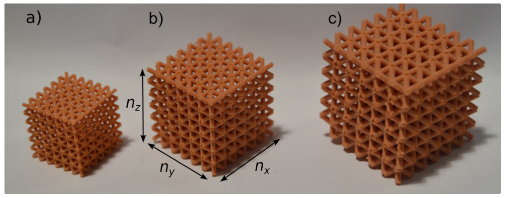
Figure 4.
Representative force–displacement curves for cubic BCC lattice specimens with different unit-cell sizes.
Figure 4.
Representative force–displacement curves for cubic BCC lattice specimens with different unit-cell sizes.
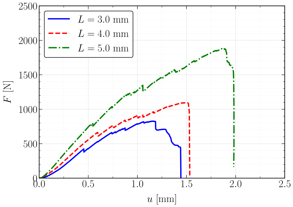
Figure 5.
Schematic representation of the three-point bending test configuration. The specimen, of total length 100 mm, rests on two cylindrical supports separated by a span of mm, while the load F is applied at mid-span through a third cylindrical roller. The bottom rollers displace upwards while the upper roller stays stationary. All loading and support rollers have a radius of mm. The vertical displacement u at the loading point is measured during the test.
Figure 5.
Schematic representation of the three-point bending test configuration. The specimen, of total length 100 mm, rests on two cylindrical supports separated by a span of mm, while the load F is applied at mid-span through a third cylindrical roller. The bottom rollers displace upwards while the upper roller stays stationary. All loading and support rollers have a radius of mm. The vertical displacement u at the loading point is measured during the test.
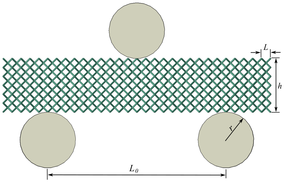
Figure 6.
Representative force–displacement curves from three-point bending tests for each unit-cell edge length considered: (a) mm, (b) mm, and (c) mm. In all cases, results are shown for beam heights of 4, 6, and 8 unit cells. Increasing beam height h produces higher stiffness and failure load, while the displacement at failure decreases accordingly.
Figure 6.
Representative force–displacement curves from three-point bending tests for each unit-cell edge length considered: (a) mm, (b) mm, and (c) mm. In all cases, results are shown for beam heights of 4, 6, and 8 unit cells. Increasing beam height h produces higher stiffness and failure load, while the displacement at failure decreases accordingly.
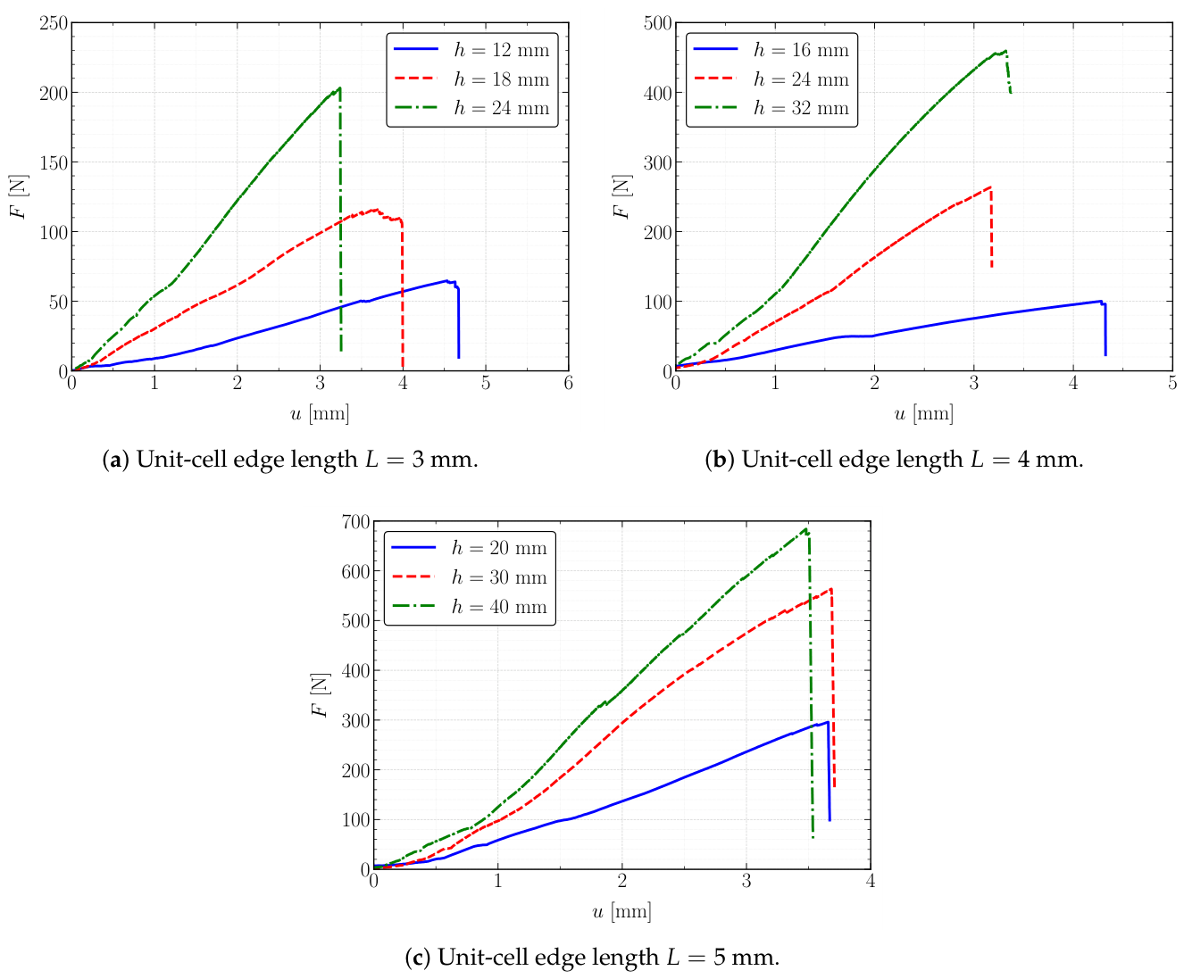
Figure 7.
Predicted versus experimental initial stiffness for the nine configurations reported in Table 3. Horizontal error bars denote the experimental standard deviation, and the dashed line indicates perfect agreement. The largest deviation corresponds to the Euler–Bernoulli prediction for the deepest beam ( mm, mm), which the shear-corrected model brings substantially closer to the experimental value.
Figure 7.
Predicted versus experimental initial stiffness for the nine configurations reported in Table 3. Horizontal error bars denote the experimental standard deviation, and the dashed line indicates perfect agreement. The largest deviation corresponds to the Euler–Bernoulli prediction for the deepest beam ( mm, mm), which the shear-corrected model brings substantially closer to the experimental value.
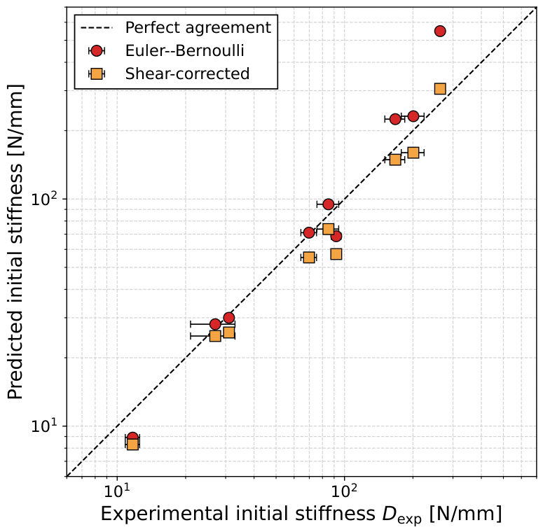
Figure 8.
Comparison of experimental initial stiffness and analytical predictions from the Euler–Bernoulli, strain-gradient Euler–Bernoulli, and shear-corrected homogenized beam models for unit-cell edge lengths (a) mm, (b) mm, and (c) mm. Error bars on experimental data represent one standard deviation. The strain-gradient parameter was calibrated as mm for mm, and for and mm.
Figure 8.
Comparison of experimental initial stiffness and analytical predictions from the Euler–Bernoulli, strain-gradient Euler–Bernoulli, and shear-corrected homogenized beam models for unit-cell edge lengths (a) mm, (b) mm, and (c) mm. Error bars on experimental data represent one standard deviation. The strain-gradient parameter was calibrated as mm for mm, and for and mm.
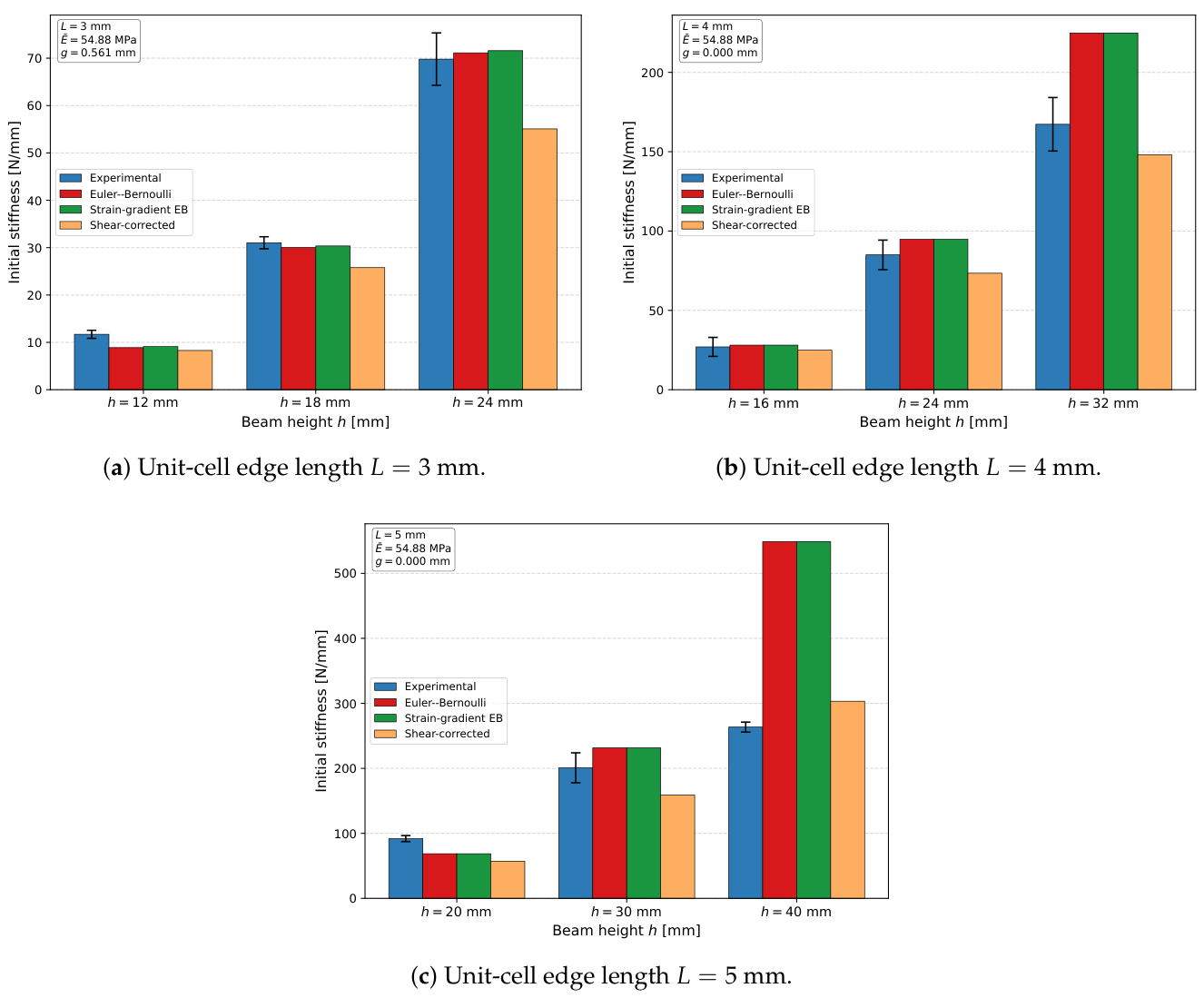
Table 1.
Homogenized cross-sectional properties—effective area and second moment of area —of the BCC lattice beam specimens as a function of unit-cell edge length L and beam height h.
Table 1.
Homogenized cross-sectional properties—effective area and second moment of area —of the BCC lattice beam specimens as a function of unit-cell edge length L and beam height h.
| L | b | h | ||
|---|---|---|---|---|
| [mm] | [mm] | [mm] | [mm2] | [mm4] |
| 12.0 | 12.0 | 144.0 | 1728.0 | |
| 3.0 | 12.0 | 18.0 | 216.0 | 5832.0 |
| 12.0 | 24.0 | 288.0 | 13824.0 | |
| 16.0 | 16.0 | 256.0 | 5461.3 | |
| 4.0 | 16.0 | 24.0 | 384.0 | 18432.0 |
| 16.0 | 32.0 | 512.0 | 43690.7 | |
| 20.0 | 20.0 | 400.0 | 13333.3 | |
| 5.0 | 20.0 | 30.0 | 600.0 | 45000.0 |
| 20.0 | 40.0 | 800.0 | 106666.7 |
Table 2.
Comparison of experimental and analytical predictions of the effective Young’s modulus for each cubic unit-cell edge length L.
Table 2.
Comparison of experimental and analytical predictions of the effective Young’s modulus for each cubic unit-cell edge length L.
| L | Experimental | Lee et al. | TD–EB | TD–Timoshenko |
|---|---|---|---|---|
| [mm] | [MPa] | [MPa] | [MPa] | [MPa] |
| 3.0 | 54.88 | 135.99 | 87.85 | |
| 4.0 | 54.88 | 135.99 | 87.85 | |
| 5.0 | 54.88 | 135.99 | 87.85 |
Table 3.
Experimental initial stiffness (mean ± standard deviation) obtained from the three-point bending tests, together with the predictions of the classical Euler–Bernoulli model and of the BCC shear-corrected homogenized beam model. Percentage errors are computed with respect to the experimental mean value.
Table 3.
Experimental initial stiffness (mean ± standard deviation) obtained from the three-point bending tests, together with the predictions of the classical Euler–Bernoulli model and of the BCC shear-corrected homogenized beam model. Percentage errors are computed with respect to the experimental mean value.
| L | h | Experimental | EB | EB error | Shear-corrected | Shear error | |
|---|---|---|---|---|---|---|---|
| [mm] | [mm] | [-] | [N/mm] | [N/mm] | [%] | [N/mm] | [%] |
| 12.0 | 6.67 | 8.9 | 24.0 | 8.30 | 29.1 | ||
| 3.0 | 18.0 | 4.44 | 30.0 | 3.3 | 25.84 | 16.7 | |
| 24.0 | 3.33 | 71.1 | 1.9 | 55.29 | 20.8 | ||
| 16.0 | 5.00 | 28.1 | 4.1 | 24.93 | 7.7 | ||
| 4.0 | 24.0 | 3.33 | 94.8 | 11.6 | 73.73 | 13.2 | |
| 32.0 | 2.50 | 224.8 | 34.4 | 148.97 | 10.9 | ||
| 20.0 | 4.00 | 68.6 | 25.4 | 57.22 | 37.8 | ||
| 5.0 | 30.0 | 2.67 | 231.5 | 15.3 | 159.96 | 20.3 | |
| 40.0 | 2.00 | 548.8 | 108.3 | 305.69 | 16.0 |
Table 5.
Root mean square error (RMSE) of the initial stiffness predictions obtained from the Euler–Bernoulli, strain-gradient Euler–Bernoulli, and BCC shear-corrected homogenized beam models. The global RMSE is computed using all nine bending configurations.
Table 5.
Root mean square error (RMSE) of the initial stiffness predictions obtained from the Euler–Bernoulli, strain-gradient Euler–Bernoulli, and BCC shear-corrected homogenized beam models. The global RMSE is computed using all nine bending configurations.
| L | Euler–Bernoulli | Strain-gradient EB | Shear-corrected |
|---|---|---|---|
| [mm] | [N/mm] | [N/mm] | [N/mm] |
| 3.0 | 1.89 | 1.85 | 9.11 |
| 4.0 | 33.70 | 33.70 | 12.46 |
| 5.0 | 166.24 | 166.24 | 39.41 |
| Global | 97.94 | 97.94 | 24.44 |
Table 6.
Mean values and standard deviations of the maximum load obtained from the three-point bending tests, as a function of unit-cell edge length L and beam height h.
Table 6.
Mean values and standard deviations of the maximum load obtained from the three-point bending tests, as a function of unit-cell edge length L and beam height h.
| L | h | |
|---|---|---|
| [mm] | [mm] | [N] |
| 12.0 | ||
| 3.0 | 18.0 | |
| 24.0 | ||
| 16.0 | ||
| 4.0 | 24.0 | |
| 32.0 | ||
| 20.0 | ||
| 5.0 | 30.0 | |
| 40.0 |
Disclaimer/Publisher’s Note: The statements, opinions and data contained in all publications are solely those of the individual author(s) and contributor(s) and not of MDPI and/or the editor(s). MDPI and/or the editor(s) disclaim responsibility for any injury to people or property resulting from any ideas, methods, instructions or products referred to in the content. |
© 2026 by the authors. Licensee MDPI, Basel, Switzerland. This article is an open access article distributed under the terms and conditions of the Creative Commons Attribution (CC BY) license (http://creativecommons.org/licenses/by/4.0/).
Copyright: This open access article is published under a Creative Commons CC BY 4.0 license, which permit the free download, distribution, and reuse, provided that the author and preprint are cited in any reuse.


