

Submitted:
09 July 2026
Posted:
17 July 2026
You are already at the latest version
Abstract
This study integrates cohort number and biological production, food consumption, feeding ecology, growth and mortality of brown trout (Salmo trutta) in Danish lowland streams monitored over long-term periods. Increasing trout density reduced instantaneous growth rate and final body size of Age-0 brown trout while increasing within-cohort variability, demonstrating strong density-dependent growth regulation. Total cohort production and food consumption increased with recruit abundance, whereas production and consumption per recruit declined strongly with increasing density, indicating reduced individual performance under crowded conditions. Despite marked interannual variation in yearly production, total yearly consumption remained comparatively stable, suggesting an upper energetic constraint imposed by prey production and stream carrying capacity. Energetic P/C ratios differed markedly between streams, averaging approximately 0.068 in BRB and 0.142 in TJB, and declined strongly with increasing body mass. Natural mortality increased with population density but decreased strongly with body mass and consumption per individual, indicating that survival was closely linked to energetic status and cumulative growth history. Feeding analyses showed that trout in both streams fed mainly on aquatic invertebrates, and prey composition overlapped substantially between streams. Overall, the results demonstrate that production, consumption, growth and mortality are tightly interconnected through density-dependent and bioenergetic mechanisms operating simultaneously at cohort and individual levels.
Keywords:
ageing
; biological production
; energetic consumption
; growth rate
; mortality
; feeding
1. Introduction
Long-term studies of brown trout population dynamics in running waters remain relatively scarce, despite their importance for understanding density-dependent regulation (e.g., Elliott & Elliott 2006; Lobón-Cerviá 2003, 2004, 2005, Lobón-Cerviá and Rasmussen 2025, Rasmussen 2018). Most existing studies are short-term (e.g., Mortensen 1977a,b,c & 1982, Mortensen 1985a; Rasmussen 1986a,b) and therefore do not adequately capture the natural interannual variability in recruitment, growth, and mortality. This is particularly important for brown trout, where recruitment is strongly influenced by stochastic variation in spring discharge during emergence, leading to substantial year-to-year variation in cohort size (e.g., Lobón-Cerviá et al. 2018).
Following recruitment, density-dependent processes regulate growth, survival, and resource use across age classes. Growth and mortality are closely linked to both fish density and food availability, and these processes interact to determine cohort trajectories. Natural mortality is generally size-dependent, declining with increasing body mass in accordance with allometric theory (Ursin 1967; Lorenzen 1996), but is also strongly influenced by resource availability and competition.
Because recruitment is largely stochastic and subsequent population dynamics are governed by density-dependent interactions, classical stock–recruitment relationships are often weak or absent in stream-resident brown trout populations (Ricker 1954; Lobón-Cerviá et al. 2018). Instead, population regulation emerges from the combined effects of variable recruitment and compensatory processes acting through growth, consumption, and mortality.
These considerations highlight the need for an integrated framework linking cohort-level processes, such as production and consumption, with individual-level mechanisms that determine growth and survival. Such an approach is essential for understanding how energy availability and density-dependent interactions propagate through the life cycle to regulate population dynamics.
Density-dependent processes are central to the regulation of salmonid populations in stream ecosystems. These processes influence growth, survival, and energy allocation, thereby linking individual-level performance to population-level dynamics. A large body of work has demonstrated that increasing density reduces growth rates and increases mortality, primarily through competition for limited resources (e.g., Elliott 1994; Elliott & Elliott 2006; Lobón-Cerviá 2007; Lobón-Cerviá & Mortensen 2005).
While the effects of density on growth and survival are well established, fewer studies have explicitly integrated density-dependent processes across multiple levels of biological organization. There is a need to link cohort-level responses, such as total production and resource consumption, with individual-level mechanisms that ultimately determine survival.
Cohort-level production and consumption typically increase with density but often exhibit diminishing returns, reflecting constraints imposed by resource limitation and habitat capacity. In contrast, individual-level responses, such as growth per recruit and consumption per individual, tend to decline with increasing density, indicating strong density-dependent competition (e.g., Jenkins et al. 1999; Grant & Kramer 1990).
Mortality, however, is rarely analysed within this integrated framework. Classical approaches have emphasised size-dependent mortality, where survival increases with body size due to reduced predation risk and improved competitive ability. This relationship has been formalised in allometric models, where mortality declines as a function of body mass (e.g., Ursin 1967, Lorenzen 1996). However, body size itself is not independent of environmental conditions but is strongly influenced by resource availability.
This suggests that mortality should not be viewed as an isolated process but rather as an emergent property resulting from the interaction between density, resource availability, and growth. In this context, consumption per individual (C/N) provides a mechanistic link between density-dependent competition and individual performance, as it directly reflects the energy available for growth and maintenance.
The objective of the present study is therefore to integrate analyses of production, consumption, and mortality within a unified framework. Specifically, we examine how recruit density influences (i) total cohort production, (ii) total cohort consumption, (iii) production and consumption per recruit, and (iv) natural mortality as a function of body size and resource availability.
We hypothesise that:
(1) cohort-level production and consumption increase with density but exhibit diminishing returns,
(2) individual-level production and consumption decline with density, and
(3) mortality decreases with both body size and consumption per individual, reflecting the combined effects of size-dependent vulnerability and energy limitation.
By integrating these processes, the study aims to provide a mechanistic understanding of how density-dependent interactions propagate from resources to growth and ultimately to survival.
2. Methods
2.1. Study Streams
Kjeldbæk (KJB), location 56.3824550 N, 9.7248830 E, is a 3.1 km stream (approximately 450 μS cm−1) and a small tributary to the River Gudenå, located approximately 5–7 km upstream of BRB and TJB (see below).
From the upper site downstream, the stream is 0.82–2.54 m wide and shallow, with mean depths ranging from approximately 11 to 15 cm and maximum depths up to about 0.4 m. Water velocities range from moderate to very fast.
The stream bed consists of a mixture of sand, gravel, and stones. Structural elements such as branches, twigs, undercut banks, and overhanging vegetation provide shelter for fish. The mean water temperature ranges from approximately 2 °C in winter to about 14 °C in summer.
Four sites, each 100 m in length, were monitored by electrofishing over a five-year period (1981–1985). Scale readings were used to assign brown trout to year classes allowing cohort-based analyses of growth, production and mortality.
Brown trout is otherwise the only fish species observed. No fishery occurs in the stream.
Brandstrup Bæk (BRB), location 62504560 N, 5505080 E, is a 4.5 km moderately to highly productive stream (approximately 450 μS cm−1) and a tributary to the River Gudenå. The stream flows through lowland agricultural areas and has relatively stable hydrological conditions.
The stream is typically 1–3 m wide, with depths generally ranging from 0.1 to 0.4 m. The substrate consists of sand, gravel, and stones, with locally abundant coarse material. Instream and marginal vegetation, together with physical structures such as undercut banks and woody debris, provide suitable shelter and feed habitats for fish.
The mean water temperature ranges from approximately 2 °C in winter to about 15–16 °C in summer. The stream supports a population of brown trout, along with occasional occurrences of few other fish species typical of Danish lowland streams.
A total of 8 sites, each 100 m long, were monitored by electrofishing over the period 1978 – 2008. Scale readings were used to assign individuals to year classes, allowing cohort-based analyses of feed, growth, production, consumption, and mortality. No fishery occurs in the study reaches.
Tjærbæk (TJB), location 62493070 N, 5535560 E, is a 7.4 km productive stream (approximately 450 μS cm−1) and a tributary to the River Gudenå. The stream flows through a mixture of meadow and agricultural landscapes and is characterised by relatively high biological productivity.
Stream width typically ranges from 1 to 3 m, with shallow depths and locally variable flow velocities. The stream bed consists of sand, gravel, and stones, and structural complexity is enhanced by vegetation, undercut banks, and organic debris, providing favourable habitat conditions for brown trout.
The mean water temperature ranges from approximately 2 °C in winter to about 15–16 °C in summer. The fish community is dominated by brown trout, along with occasional occurrences of few other species typical of Danish lowland streams.
A total of 14 sites, each 100 m long, were monitored by electrofishing over the period 1981 - 1996. Scale readings were used to separate fish into year classes, enabling detailed cohort analyses of feed, production, consumption, and mortality. No fishery occurs in the study reaches.
2.2. Sampling, Ageing and Growth
Electrofishing was conducted from spring to autumn and during the sea trout spawning run using a pulsed DC current (400 V). All captured brown trout were anaesthetised in a 0.03 g L−1 benzocaine solution, and total length was measured to the nearest 0.5 cm. Samples of trout were weighed (g wet wt.) in the laboratory. Each sampling section was electrofished up to three consecutive times following the removal method described by Bohlin et al. (1989).
Scale reading was used to assign individuals (parr, smolts and sea trout) to year classes. The designation R refers to recruits in mid-April, 0+ refers to the first-year class sampled in November. The classes 1+ to 4+ represent older year classes in November originating from previous cohorts. Age-0 refers to the period from recruitment to mid-November, and Age-1, Age-2 and Age-3 refer to the period from mid-November to mid-November the following year.
A cohort, also termed a year-class, comprises the recruits entering the population each year and subsequently followed through successive age classes until the cohort becomes extinct. In any given year, the fish population comprises individuals from different age groups originating from different cohorts.
2.3. Calculation of Mean Body Mass (g Wet wt.) and Mean Length (cm)
Mean body mass (MBM) of the first year class from recruitment (R) to 0+ in November was calculated as MBM = 0.1549 (exp(G) − 1) / G, where the body mass (BM) of a recruit is 0.1549 g wet wt. and the instantaneous growth rate is defined as G = ln(0+ BM / 0.1549) (Chapman 1978).
Mean body mass of the following three year classes was calculated in the same way where the mass of a recruit R was exchanged with body masses of 0+, 1+, 2+ and 3+, and G was recalculated with the new data.
The mean number (MN) of brown trout within a year (7 months for the first year class, R → 0+) was calculated as N_mean = N_R (exp(-M) − 1) /-M, where M is the natural mortality over 7 months (Chapman 1978).
For older year classes, the mean number was calculated as N_mean = N_i (exp(M) − 1) / M, where the annual mortality rate (12 months) is given by M = ln(N_i+1 / N_i).
These calculations were performed for all cohorts and year classes, and the total number of brown trout was summed for each year.
The natural instantaneous mortality rate (M) for the first year class was estimated from mid-April (recruitment, R) to number of 0+ in mid-November as M = −ln(R / 0+).
2.4. Feeding
A smaller number of brown trout were sampled by electrofishing in Brandstrup Bæk (BRB) and Tjærbæk (TJB), and stomach contents were analysed to identify prey taxa.
Stomach samples (273) collected over three study years were distributed across months. The first samples were obtained in February and the last in December. Stomach contents were weighed to the nearest 0.01 g (wet wt.) and identified to the lowest possible taxonomic level.
Number of occurrences (NoC) was calculated as the proportion of individuals containing a given prey item relative to the total number of individuals with stomach contents. Some prey taxa were measured to the nearest 0.1 cm in length.
BRB
A total of 154 brown trout (5–21 cm) were collected between 6 February and 6 November 1985. Some of the most important taxa were measured for length.
The number of stomachs examined was insufficient to allow a detailed analysis of diet composition in relation to age or body length. Therefore, all fish sizes were pooled.
TJB
A total of 119 brown trout (5–15 cm) were collected between 6 April and 14 December 1985. Stomach contents were analysed in the same way as for BRB.
As in BRB, the sample size was too limited to allow analysis of diet composition in relation to age or body length, and all fish sizes were therefore pooled.
2.5. Biological Production and Consumption
Biological production was calculated as MBM MN Individual food consumption, see below, was calculated using the relationship between food content g wet wt. in brown trout stomachs. The mean size of 273 analyzed brown trout stomach with different invertebrate taxa was calculated to 23.8 g wet wt. ranging from 1.1 g up to 110.9 g wet wt. The relationship between stomach content and brown trout body mass BM was described as:
We assume that the mean annual water temperature in BRB and TJB is 7.6 0C (Rasmussen 2018).
The evacuation rates in Elliott (1972) with water temperatures in the range of 5.2 – 15.0 0C was calculated independent of brown trout body mass and depends only on water temperature, and influence of fish body mass was not included. Stomach content was proportional to trout body mass, but the feeding consumption used for growth and respiration will always be proportional to trout body mass (2/3 – 3/4) (Jobling 1994). To keep a constant proportional relationship between trout body mass and stomach content, the logical conclusion might be that the evacuation rate depends on trout body mass. In contrast to Elliott (1972) other results (e.g., Tseitlin 1980) suggest that evacuation rate (for a given temperature) also depends on body mass of a fish, so that resulting feeding rate and food consumption of small fish is relatively higher compared to bigger fish. The conclusion is that the calculation of maximum food consumption in Elliott (1975) is slightly biased. We used Elliott (1972) but incorporated a size dependent evacuation rate to estimate the true body mass dependent food consumption using the stomach content given in relationship (1).
Production and consumption were analysed using logarithmic models, while mortality was analysed using a log-linear model including body mass and consumption per individual (C/N). All variables were log-transformed. Model diagnostics included residual analysis and variance inflation factors.
Relationships between recruit density and cohort-level responses (total cohort production and total cohort consumption) were analysed using logarithmic regression models.
Per-capita responses (production per recruit and consumption per recruit) were analysed using power-function models fitted as linear regressions on log-transformed data
2.6. Data Treatment
The results were calculated and tested, using Excel ver. 5.0, Real Statistics Resource Pack version 6.7, and http://statpages.org/nonlin.html. The level of significance for statistical tests was 0.05. Figures were made in Matplotlib ver. 3.9.2. Power functions were fitted in log–log space. Back-transform intercepts were corrected for retransformation bias as , where is the fitted intercept and is the residual variance in log space.
3. Results
3.1. Length and Body Mass
In Figure 1, the relationships between mean body mass (g wet wt.) and mean total length (cm) versus age groups using the total number of observations of the whole data set.
The figure demonstrates the strong ontogenetic increase in both body mass and total length with increasing age. At all age groups, brown trout from TJB attain larger body mass and greater total length than trout from BRB, and the divergence between streams increased progressively from Age-1 to Age-3.
3.2. Length and Instantaneous Growth Rate G of 0+ Versus Number of 0+-4+
In Figure 2 is shown the relationships between total length cm of 0+ of BRB and TJB in November (i.e., end of growth) versus number of 0+-4+, and the relationship between daily instantaneous growth rate G between size of recruits R (2.5 cm) in April and size of 0+ in November. Each observation represents mean length and mean G from all sites.
The upper panels Figure 2a,b show the relationships between mean total length of 0+ trout and total trout density in BRB and TJB, respectively. In both streams, mean length declined significantly with increasing density, demonstrating clear density-dependent growth regulation. The relationships were described by power functions fitted in log–log space and back-transformed to the original scale.
In BRB (panel a), the relationship was:
- with , , and .
In TJB (panel b), the relationship was:
- with , , and .
The lower panels Figure 2c,d show the relationships between instantaneous growth rate of 0+ trout and total trout density in BRB and TJB, respectively. Instantaneous growth rate also declined significantly with increasing density in both streams, indicating that density-dependent suppression acts directly on the growth process itself.
In BRB (panel c), the relationship was:
- with , , and .
In TJB (panel d), the corresponding relationship was:
- with , , and .
In all panels, density-dependent responses were substantially stronger in BRB than in TJB. The close similarity between the exponents estimated for mean length and instantaneous growth rate indicates that the density-dependent reduction in body size is fundamentally driven by reduced instantaneous growth rate under high-density conditions.
Thus, increasing density was associated with reduced mean length of 0+ trout in both streams, but the relationship was markedly stronger in BRB, where density explained a substantially larger proportion of the variation in length.
The difference in slopes between streams was tested by ANCOVA in log–log space. The interaction between log(density) and site was significant , demonstrating that the density–length relationship was significantly steeper in BRB than in TJB. This confirms that density-dependent growth operates more strongly in BRB.
To evaluate whether density-dependent growth of age 0+ trout was primarily associated with the total trout population or specifically with older fish, additional analyses were performed using only the density of trout aged 1+–4+ per 100 m2 as the explanatory variable.
Mean total length of 0+ trout declined significantly with increasing density of older trout in both BRB and TJB. In BRB, the relationship was described by the power function:
- with , , and .
In TJB, the corresponding relationship was:
- with , , and .
Instantaneous growth rate also declined significantly with increasing density of older trout. In BRB, the relationship was:
- with , , and .
In TJB, the corresponding relationship was:
- with , , and .
Thus, increasing density of older trout alone was associated with reduced growth performance of age 0+ trout in both streams. However, the explanatory power of these relationships was consistently lower than in the analyses using total trout density (0+–4+), particularly in BRB. This indicates that although older trout contribute substantially to density-dependent suppression of growth, the density of the 0+ year class itself contributes importantly more to the overall density effect.
The negative exponents in both systems indicate that instantaneous growth rate decreased continuously with increasing density. However, the stronger exponent and higher in BRB demonstrate a substantially tighter coupling between growth and density in this stream.
Overall, the results show that density-dependent suppression of growth occurred in both systems but was markedly stronger and more consistently expressed in BRB.
3.3. Coefficient of Variation CV% of 0+ vs Length of 0+ and Number 0+-4+.
The coefficient of variation (CV%) is a measure of the individual variation in salmonids and used to demonstrate density dependent growth (e.g., Elliott 1994 & 2015, Jenkins et al. 1999, Lobon-Cervia 2010, Richard et al. 2015).
In Figure 3 is shown the relationships between CV%s of age 0+ in November (i.e., end of growth) of BRB and TJB versus length og 0+ and number of 0+.-4+.
The upper panels Figure 3A,B show the relationships for BRB, whereas the lower panels (c–d) show the corresponding relationships for TJB. Panels a and c describe the relationships between CV% 0+ and mean length of 0+ trout, while panels b and d show the relationships between CV% 0+ and total 0+–4+ trout density.
In BRB (panel a), CV% declined strongly with increasing mean length:
- with , , and .
In BRB (panel b), CV% increased with increasing total density:
- with , , and .
In TJB (panel c), CV% also declined with increasing mean length:
- with , , and .
In TJB (panel d), CV% increased with increasing density:
- with , , and .
Overall, increasing density was associated with increased within-cohort variability, whereas increasing mean length 0+ was associated with reduced variability. Both relationships were substantially stronger in BRB than in TJB, indicating tighter density-dependent regulation of cohort structure in BRB.
Thus, cohorts with larger mean length were consistently more homogeneous, showing lower relative variation. However, the strength of this relationship differed markedly between streams. In BRB, mean length explained nearly half of the variation in CV%, whereas in TJB the relationship was weak, indicating greater unexplained variability.
Thus, higher density was associated with increased variability within the cohort. As in panel a, the relationship was stronger in BRB than in TJB.
ANCOVA performed in log–log space demonstrated significant differences in slopes between BRB and TJB for both relationships.
For the CV%–length relationship (panels a and c), the interaction between log(length) and site was highly significant , indicating that the decline in CV% with increasing length was substantially steeper in BRB than in TJB.
For the CV%–density relationship (panels b and d), the interaction between log(density) and site was also significant , demonstrating that the increase in CV% with density was significantly stronger in BRB than in TJB.
Taken together, Figure 3 demonstrates two consistent and complementary patterns: CV% decreases with increasing mean length of 0+ and increases with increasing density of 0+-4+, and both relationships are substantially stronger in BRB than in TJB.
3.4. Biological Production, Food Consumption, Energetic Efficiency P/C and Natural Mortality M
Recruit and Biological Production
In Figure 4 the relationships between total cohort production g wet wt. in relation to number of recruits and production per recruit in relation to number of recruits of the cohorts is shown for BRB and TJB. KJB is only given for observations.
The relationship between total cohort production (P) and the number of recruits (N) was described by a logarithmic model of the form P = a + b · ln(N) (Figure 4a). For BRB, the fitted parameters were a = −1790.261 and b = 547.940 (R2 = 0.76, p = 0.000), whereas for TJB (Figure 4b), a = −418.764 and b = 383.602 (R2 = 0.83, p = 0.000).
Production per recruit (P/N) declined with increasing recruitment and was described by a power-function model of the form P/N = a · Nb (Figure 4b). For BRB, the fitted parameters were a = 42.451 and b = −0.400 (R2 = 0.58, p = 0.000), whereas for TJB, a = 199.235 and b = −0.571 (R2 = 0.93, p = 0.000).
The additional KJB observations generally followed the same overall relationship between recruit abundance and total cohort production as observed by BRB and TJB (Figure 4). In panel (a), the KJB observations largely overlapped the BRB production trajectory, and in panel (b) the KJB values for production per recruit followed the same relationship as BRB. Overall, the KJB data therefore supported the general pattern of increasing total cohort production but declining production per recruit with increasing recruit abundance.
Annual Biological Production
In Figure 5 is shown annual production of four year classes and total annual production g wet wt. in BRB and TJB in years 1981 to 1998.
Annual production of brown trout cohorts in the two streams BRB (Panel a) and TJB (Panel b). Separate curves are shown for Age-0, Age-1, Age-2, Age-3, and total annual production summed across all cohorts. The black curve represents total annual production, whereas coloured curves represent age class specific production. Considerable interannual variation occurred in both streams, although BRB generally showed substantially higher production levels and stronger temporal fluctuations than TJB. In both streams, Age-1 and Age-2 cohorts contributed most to total production, whereas Age-3 production was comparatively lower and more variable over years.
Substantial interannual variation in yearly production was observed in both BRB and TJB (Figure 5). Total annual production in BRB varied from approximately 829 to 1739 units (i.e., g wet wt.), whereas total production in TJB ranged from approximately 556 to 1453 units. Overall, BRB exhibited consistently higher production levels than TJB during most years of the study period.
In BRB, the temporal dynamics of total production were characterized by pronounced fluctuations, with particularly high production during 1989–1991 and again in 1995–1996. The highest total annual production occurred in 1991 (1739 units), closely followed by 1989 (1704 units). In contrast, markedly reduced production occurred in 1994 (829 units). The Age-1 cohort contributed strongly and consistently to total production throughout the study period and often represented the dominant cohort. Age-2 production also contributed substantially, particularly during years with elevated total production, whereas Age-0 and Age-3 cohorts showed greater year-to-year variability.
In TJB, yearly production was generally lower and less variable than in BRB. Nevertheless, a pronounced production peak occurred in 1987, when total production reached 1453 units. Following this peak, total production declined substantially, particularly during 1988–1993, where yearly totals frequently remained below 1000 units. Like BRB, Age-1 and Age-2 cohorts contributed most strongly to total production, whereas Age-0 production remained comparatively low throughout the study period.
The temporal patterns further indicated that variation in total production was largely driven by fluctuations in intermediate cohorts, especially Age-1 and Age-2 fish. In contrast, production by older Age-3 trout contributed relatively little to total production in most years despite occasional increases in specific years.
A diagnostic analysis (i) temporal variation in total yearly production in BRB showed, despite substantial interannual fluctuations, no significant R2 = 0.009 and p = 0.708 long-term directional trend. (ii) residuals in BRB fluctuated around zero without evidence of systematic temporal structure, supporting the interpretation of random interannual variation. (iii) The lag-1 relationship between total production in year t and production in year t+1 in BRB, the weak and non-significant correlation indicates low temporal persistence between consecutive years. (iiii) None of the autocorrelation coefficients in BRB exceeded the confidence limits, indicating absence of significant temporal autocorrelation and supporting the interpretation that annual production fluctuated stochastically around a relatively stable long-term mean.
Together, these results support the interpretation that BRB production fluctuated around a relatively stable mean rather than following a persistent temporal trend.
Food Consumption and Energetic Efficiency P/C in relation to Number of Recruits
In Figure 6 the relationships are shown between cohort consumption (g wet wt.) and consumption per recruits of BRB and TJB versus number of recruits.
The relationship between total cohort consumption (C) and the number of recruits (N) differed between the two stream systems, but in both cases was adequately described by a logarithmic model of the form C = a + b · ln(N) (Figure 6a). For BRB, the fitted parameters were a = −9918.346 and b = 5382.924, with the model explaining 41% of the variation in total consumption (R2 = 0.41, p = 0.001). For TJB, the corresponding fitted parameters were a = 2100.675 and b = 1641.307, and the model explained 50% of the variation (R2 = 0.50, p = 0.023). Thus, total cohort consumption increased with increasing recruitment in both streams, but the increase was much steeper in BRB than in TJB, resulting in substantially higher total consumption at moderate to high recruit abundances.
Consumption per recruit (C/N) declined with increasing recruitment and was described by a power-function model of the form C/N = a · Nb (Figure 6b). For BRB, the fitted parameters were a = 3079.823 and b = −0.670, with the model explaining 71% of the variation in consumption per recruit (R2 = 0.71, p = 0.000). For TJB, the fitted parameters were a = 3601.915 and b = −0.783, and the model explained 91% of the variation (R2 = 0.91, p = 0.000). These results show that per capita consumption declined strongly with increasing recruitment in both systems, but that the decline was steeper and more tightly constrained in TJB than in BRB.
Taken together, the two panels indicate a consistent density-dependent pattern: increasing recruit abundance was associated with higher total cohort consumption, but with lower consumption per recruit. At low recruit densities, especially in TJB, individual recruits exhibited high consumption rates, whereas at higher recruit densities total cohort consumption increased while the average contribution per recruit declined markedly.
In contrast to annual production, total annual consumption exhibited comparatively limited interannual variability in both BRB and TJB (Figure 7). In BRB, total yearly consumption varied between approximately 15,350 and 21,860 units per 100 m2, whereas TJB varied between approximately 5,627 and 9,786 units per 100 m2. Although fluctuations among individual year classes were substantial, total consumption remained remarkably stable through time relative to the corresponding variation observed for yearly production.
Visual inspection of the time series suggested little evidence of strong temporal instability or directional change in total yearly consumption. In BRB, total consumption remained consistently centred around approximately 18,000–21,000 units per 100 m2 during most years of the study period, despite pronounced fluctuations in the relative contributions of individual age groups. Similarly, TJB showed relatively stable total consumption levels around approximately 8,000–10,000 units per 100 m2 during most years, although a decline occurred during the final years of the series.
The relatively stable total consumption contrasted markedly with the stronger year-to-year fluctuations observed for yearly biological production. Year class specific consumption appeared to compensate among age groups. Years with reduced consumption in one year class were frequently associated with increased consumption in other year classes, thereby stabilizing total annual consumption.
Age-2 trout generally contributed most strongly to total yearly consumption in both streams, followed by Age-1 and Age-3 fish, whereas Age-0 trout contributed comparatively little despite occasionally high recruitment densities. Thus, total yearly consumption appeared to be dominated primarily by intermediate and larger trout cohorts.
The overall temporal pattern suggests that total annual food consumption was constrained within a relatively narrow range despite substantial variation in cohort structure and yearly biological production.
Energetic Production-to-Consumption ratio P/C of BRB and TJB
In Figure 8 is shown the energetic production-to-consumption ratio (P/C) and the number of recruits (N), and body mass (g wet wt.) of brown trout in BRB and TJB.
To ensure direct comparability between production and consumption, both variables were converted to energy units. Production was converted using 1.3002 Kcal g−1 wet wt. for brown trout, and consumption using 1.061 Kcal g−1 wet wt. for Gammarus. The resulting energetic production-to-consumption ratio (P/C) was analysed in relation to recruitment (N) and followed a logarithmic model of the form P/C = a + b · ln(N). For BRB, the fitted parameters were a = −0.031 and b = 0.019 (R2 = 0.45, p < 0.001), whereas for TJB, a = 0.039 and b = 0.030 (R2 = 0.42, p = 0.044).
The mean energetic P/C ratio for all observations combined was 0.090. However, marked differences were observed between the two stream systems. BRB averaged 0.068, whereas TJB exhibited a substantially higher mean value of 0.142. These results demonstrate that P/C is not a universal constant but varies both with recruitment density and between stream systems.
Energetic production-to-consumption ratios (P/C) differed markedly between the two stream systems and showed clear relationships with both recruit abundance and body mass (Figure 8A,B).
In Figure 8A, energetic P/C increased with increasing number of recruits in both streams, although the relationships differed substantially between BRB and TJB. In BRB, energetic P/C values were generally low and ranged approximately from 0.03 to 0.10, with a gradual increase at increasing recruit abundance. In contrast, TJB exhibited consistently higher energetic P/C ratios, typically between 0.10 and 0.19, despite substantially lower recruit abundances. The fitted relationships therefore indicate that trout populations in TJB converted consumed energy into fish production more efficiently than populations in BRB across the observed range of recruit densities.
Figure 8B demonstrated a strong allometric decline in energetic P/C with increasing body mass. Energetic P/C was highest in Age-0 trout and decreased progressively through Age-1, Age-2 and Age-3 fish. The decline followed a negative power-type relationship between body mass and energetic P/C, indicating reduced energetic conversion efficiency with increasing fish size. This ontogenetic pattern was evident in both stream systems, although TJB consistently exhibited higher energetic P/C ratios than BRB at comparable body masses and age groups.
The statistical analyses demonstrated that body mass alone explained a large proportion of the variation in energetic P/C. A log-log regression model showed a highly significant negative relationship between body mass and energetic P/C . Inclusion of stream identity significantly improved the model fit, demonstrating that TJB consistently exhibited higher energetic P/C values than BRB after correction for body mass . Addition of age group explained further variation, although much of the ontogenetic pattern was already incorporated through the strong body mass dependence. The interaction between stream and body mass was weak and non-significant, indicating that the overall slopes were broadly similar between streams, whereas the principal difference was a systematic upward displacement of the TJB relationship relative to BRB.
Overall, the combined analyses indicate that energetic conversion efficiency in stream-resident brown trout was regulated both by population-level processes associated with recruit abundance and by individual-level bioenergetic scaling related to body size and ontogenetic development.
Mortality in relation to Density, Consumption, and Body Mass
In Figure 9 the relationships are shown between (i) natural daily mortality (M) of Age-0 versus density of Age-0 .- Age-3 (panel a), (ii) total food consumption of Age-0 .- Age-3 (panel b) and (iii) body mass g wet wt of Age-0 (panel c).
Natural mortality (M) increased with both density and consumption but decreased with increasing body mass. Body mass provided the strongest explanatory variable among the tested predictors.
Natural mortality (M) of Age-0 brown trout was significantly related to total population density, total consumption, and body mass (Figure 9). In all analyses, locality (BRB vs TJB) was included as an additive factor, and no significant interaction between predictor variables and locality was detected, indicating that the slopes of the relationships were consistent across the two stream systems.
Mortality increased significantly with total population density (Age-0 to Age-3), and the relationship was well described by a linear model of the form , where Locality = 1 for BRB and 0 for TJB. Total density was a highly significant predictor of mortality () and explained a substantial proportion of the variation (). At comparable densities, mortality was consistently higher in BRB than in TJB, as reflected by the positive locality coefficient.
A nearly identical pattern was observed for total consumption Ctot (Age-0 to Age-3). Mortality increased significantly with increasing consumption, following the relationship . Total consumption was also highly significant () and explained a similar proportion of the variation in mortality (). The close correspondence between the density- and consumption-based models indicates that these variables capture similar aspects of population-level pressure.
In contrast, mortality decreased significantly with increasing body mass of Age-0 individuals. This relationship was described by the model , in which body mass had a strong negative effect on mortality () and locality remained significant (). This model explained the largest proportion of the observed variation (), indicating that body mass was the strongest predictor among the variables tested.
Comparison of model performance showed that body mass provided a better explanation of mortality than either density or consumption, whereas the latter two variables exhibited nearly identical explanatory power. Thus, although mortality was clearly related to population-level variables such as density and consumption, it was most directly associated with individual body size.
Finally, alternative model formulations, including log-transformed and saturation-type models, did not improve the fit relative to the linear models. This indicates that, within the observed range of densities and consumption levels, mortality increased approximately proportionally with population pressure and decreased proportionally with body mass.
Body mass provided the strongest explanatory variable, indicating that mortality is most directly related to individual size rather than population-level variables. I.e.
Linear models provided the best description of the data. Neither log-transformed nor saturation-type models improved model fit, indicating approximately proportional relationships within the observed range.
3.5. Feeding
The feeding results are given in Table 1.
A PERMANOVA based on Bray–Curtis dissimilarities showed no significant difference in prey composition between streams (R2 = 0.08, p = 0.203). Stream identity explained only a small proportion of the total variance, indicating that spatial differences were minor compared to temporal variability.
Ordination analysis (NMDS) revealed a high degree of overlap between samples from BRB and TJB, with no clear separation between streams. In contrast, substantial variation was observed between sampling months.
Despite the lack of an overall stream effect, certain taxa showed consistent differences. Plecoptera were largely absent in TJB but occurred regularly in BRB. Similarly, Asellus differed in abundance between streams.
BRB
The most important taxa were Chironomidae larvae and adult and other Diptera larvae and adult, Trichoptera larvae (Limnephilidae, Rhyacophila, Hydropsyche and Oligopentrum) and Plecoptera nymphs. Secondarily there was Simulidae larvae, Ephemeroptera nymphs and Gammarus pulex. Beside these taxa were Lepidoptera larvae, Neuroptera nymphs, Odonata larvae, Heteroptera, Hymenoptera adults, Arachnida and Gastropoda. One single lamprey was eaten in November. Brown trout eggs were eaten in February and November. The sizes of Ephemeroptera, Trichoptera and Plecoptera were independent of brown trout length (p < 0.05). For Gammarus pulex there was an increase in prey size versus the length of brown trout.
TJB
The most important taxa were Ephemeroptera nymphs, Tricophtera larvae, Chironomidae larvae, other Diptera larvae including Simulium larvae, Gammarus pulex, Asellus aquaticus and Coleoptera larvae and adults. Plecoptera nymphs, Lepidoptera larvae, Hymenoptera imago, Arachnida, Lumbricidae and Gastropoda terrestrial were of secondary importance.
4. Discussion
4.1. Length, Density-Dependent Growth and Cohort Structure
The combined analyses of mean body mass and length of 0+ trout (Figure 1) and instantaneous growth rate in relation to age and total trout density (Figure 2) provide a consistent picture of density-dependent growth regulation in both BRB and TJB. In both streams, increasing total trout density was associated with reduced mean length and reduced instantaneous growth rate of Age-0 trout. This indicates that density-dependent suppression acts directly on the growth process itself and is subsequently expressed as reduced final body size at the end of the first growing season.
The close correspondence between the density–growth and density–length relationships is important. Instantaneous growth rate describes the physiological process of biomass accumulation, whereas mean length represents the cumulative outcome of that process. The fact that both variables declined with increasing density therefore shows that reduced final size was not merely a statistical pattern, but the consequence of reduced somatic growth under high-density conditions.
The relationships were consistently stronger in BRB than in TJB. In BRB, density explained a larger proportion of the variation in both growth rate and mean length, indicating tighter density-dependent regulation. In TJB, the same negative relationships were present, but with weaker explanatory power, suggesting that density-dependent growth regulation was partly masked by additional environmental variability. Such variability may include differences in discharge, habitat structure, prey availability, recruitment timing or local temperature conditions.
The analysis including only older trout densities showed that Age-1 to Age-3 trout also contributed to reduced growth performance of Age-0 trout. However, these relationships were weaker than those based on total trout density. This indicates that inter-cohort competition from older trout is important, but that intra-cohort competition among Age-0 fish also contributes substantially to the overall density effect. Thus, density-dependent growth regulation in these streams should be interpreted as the combined result of competition within the Age-0 cohort and competitive interactions with older trout.
The relationships (Figure 3) between CV% of Age-0 trout, mean length and density further support this interpretation. CV% declined with increasing mean length and increased with increasing density, especially in BRB. High-density cohorts were therefore not only smaller on average, but also more heterogeneous. This suggests that competition increases asymmetry among individuals, probably because some fish obtain better feeding positions or shelter, whereas others are forced into less profitable microhabitats. Density dependence therefore affects both mean growth and the internal size structure of the cohort.
Overall, the growth and CV% analyses support a coherent model in which increasing density reduces instantaneous growth, reduces final body size and increases within-cohort variability. These effects were strongest in BRB, indicating that BRB behaved as a more tightly density-regulated system, whereas TJB appeared more influenced by additional environmental variation.
4.2. Production in Relation to Recruitment
The production analyses (Figure 4) showed that total cohort production increased with the number of recruits in both streams, up to about 20 g wet et per 1 m2 and followed logarithmic relationships, and that annual production varied approximately 8 - 18 g wet wt. per 1 m2.
Earlier Danish studies by Mortensen (1977a,b,c,d; 1982; 1985a,b) demonstrated considerable variation in brown trout production among streams, with annual production ranging from approximately 5 to 33 g wet wt. per m2. The studies showed that stream productivity depended strongly on recruitment success, trout density, growth rates, and benthic invertebrate production, with the most fertile Danish streams among the most productive brown trout systems reported in Europe. Javier and Rasmussen (2025) proposed that annual brown trout production (Danish, English and Spanish rivers combined) might have a maximum limit at approximately 40-45 g wet wt. per 1 m2. Thus, increasing recruitment resulted in higher total production, but with diminishing marginal gains at high recruit abundance. This pattern is biologically consistent with density-dependent regulation: more recruits generate more total biomass production, but each additional recruit contributes progressively less as food resources, space and profitable feeding positions become limiting.
The fitted relationships differed between the streams. BRB had the steeper increase in total cohort production with recruitment, indicating that high recruit abundance translated into relatively high total production in this stream. TJB had lower recruit abundance but higher production per recruit. Thus, BRB was characterized by high total cohort output driven by greater numbers, whereas TJB was characterized by higher individual performance.
Production per recruit declined with increasing recruitment in both streams. This confirms that density dependence was already expressed at the level of individual performance. The decline was especially strong and well defined in TJB, where the power-function relationship explained a very large proportion of the variation. This means that although TJB had higher production per recruit at low densities, individual production was strongly reduced when recruitment increased.
These results explain why early similarities in length or body mass between streams do not necessarily lead to similar production patterns. Cohort production integrates both individual growth and cohort abundance. Small differences in body size may be amplified when converted to body mass, and total cohort production is further modified by the number of surviving individuals. Therefore, BRB can show higher total production because of greater abundance, while TJB can show higher production per recruit because of lower density and better individual growth.
The temporal production analyses showed substantial interannual variation in both streams. In BRB, total yearly production varied markedly, but the diagnostic analyses showed no significant long-term trend, no significant lag-1 autocorrelation and no evidence of strong temporal persistence. Yearly production therefore fluctuated around a relatively stable long-term mean rather than following a directional temporal change.
This is important biologically. The production peaks and troughs should not be interpreted as evidence of progressive improvement or deterioration of the stream. Instead, they most likely reflect year-to-year variation in recruitment, survival, growth conditions, discharge, temperature and food availability. Age-1 and Age-2 trout contributed most to total yearly production in both streams because these year classes combined relatively high abundance with substantial body mass accumulation. Age-0 trout contributed less because of small body size, whereas Age-3 trout contributed less because abundance had already been reduced by cumulative mortality.
4.3. Consumption and Annual Energetic Constraint
The consumption analyses closely paralleled the production results. Total cohort consumption increased (Figure 6a) with recruitment in both BRB and TJB but again followed logarithmic relationships. Thus, larger cohorts consumed more food in total, but total consumption did not increase proportionally with the number of recruits. This indicates that food acquisition became progressively constrained as recruit abundance increased.
Consumption per recruit (Figure 6b) declined strongly with increasing recruitment in both streams. This provides direct mechanistic support for the production patterns. Reduced production per recruit at high density is therefore not simply a demographic result but is linked to reduced food intake per individual. The decline in consumption per recruit was especially strong in TJB, whereas BRB showed a steeper increase in total cohort consumption with recruitment. This indicates that BRB could sustain higher total food uptake at high recruit abundance, whereas individual consumption in TJB was more tightly constrained by density.
The yearly consumption (Figure 7) analysis adds an important temporal perspective. In contrast to yearly production, total yearly consumption varied within a relatively narrow range in both streams. In BRB, total yearly consumption remained approximately within 15,350–21,860 units per 100 m2, whereas TJB varied approximately within 5,627–9,786 units per 100 m2. Although individual age groups fluctuated substantially, total annual consumption was comparatively stable.
This suggests that the streams may have supported a relatively stable long-term prey production or energetic supply. The trout population did not simply consume in direct proportion to year class abundance. Instead, consumption appeared to be redistributed among age groups, so that reductions in one year class were partly compensated by increases in others. Such compensation is consistent with density-dependent regulation and flexible trophic partitioning among cohorts.
The contrast between variable production and comparatively stable consumption is central. Annual production fluctuated because recruitment strength, mortality, growth efficiency and year class composition varied among years. Total consumption, however, appeared more closely constrained by the long-term food base of the stream. Therefore, variation in production may reflect not only variation in the amount of food consumed, but also variation in how efficiently consumed energy was converted into trout biomass.
4.4. Energetic P/C Ratio
The energetic production-to-consumption ratio provides a useful synthesis (Figure 8) of these processes. When production and consumption were converted to comparable energy units, the mean energetic P/C ratio across all observations was 0.090. However, the two streams differed markedly: BRB averaged 0.068, whereas TJB averaged 0.142. Thus, P/C was not a universal constant, but varied both between stream systems and with ecological conditions.
The BRB value (Figure 8A) was close to the previously estimated annual P/C ratio of approximately 0.067. After correction for differences in energy content between trout tissue and Gammarus prey, this corresponds approximately to 0.082 for BRB-type data. The overall energetic mean of 0.090 is higher because it includes TJB, where energetic conversion efficiency was substantially greater. The distinction is important: 0.067–0.068 describes the BRB level, whereas 0.090 describes the combined energetic mean, and 0.142 describes the higher TJB level.
The higher P/C ratio (Figure 8A) in TJB indicates that trout in this stream converted consumed energy into fish production more efficiently than trout in BRB. This may reflect lower density, higher individual growth, different prey availability, lower metabolic costs, or habitat conditions that allowed more efficient feeding. Conversely, the lower P/C ratio in BRB is consistent with higher density, stronger competition and greater energetic costs associated with maintaining populations at higher abundance.
The relationship (Figure 8A) between P/C and body mass provides a mechanistic explanation for part of this variation. Energetic P/C declined with increasing body mass, being highest in Age-0 trout and progressively lower in older and larger trout. This is consistent with bioenergetic theory: small fish allocate a larger proportion of consumed energy to somatic growth, whereas larger fish allocate relatively more energy to maintenance metabolism, activity and respiration. Body mass therefore appears to be a more fundamental explanatory variable than age itself, because much of the age effect is mediated through increasing size.
The broadly similar body-mass scaling (Figure 8B) in the two streams indicates that the underlying allometric mechanism was comparable. The main difference was that TJB had a consistently higher energetic level. Thus, the stream difference in P/C does not imply fundamentally different bioenergetic scaling, but rather different ecological conditions under which the same scaling process operated.
4.5. Mortality in Relation to Density, Consumption and Body Mass
The mortality analyses (Figure 9) connect density-dependent growth, consumption and energetic efficiency directly with survival. Natural mortality M of Age-0 trout increased with total trout density and with total population consumption but decreased with increasing body mass. Among the single-predictor relationships, body mass provided the strongest explanation of mortality. This indicates that mortality was most directly linked to individual size, even though population-level pressure from density and total consumption was also important.
The positive relationships between mortality and total density (Figure 9a) or total consumption (Figure 9b) should be interpreted as indicators of population-level pressure. High density increases competition for food, shelter and profitable feeding positions. High total consumption reflects a large collective demand on the food base. Both variables therefore describe situations in which the population places strong pressure on available resources. Under such conditions, smaller or competitively inferior Age-0 trout are likely to experience reduced growth, lower energetic reserves and higher mortality.
The negative relationship between mortality and body mass is consistent with allometric mortality theory. Larger Age-0 trout are less vulnerable because they have greater energy reserves, improved swimming capacity, better competitive ability and probably lower predation risk. Conversely, small individuals are more sensitive to starvation, displacement and winter mortality. The strong explanatory power of body mass therefore supports the view that mortality is partly mediated through growth history.
It is important to distinguish total consumption from consumption per individual. Total consumption increased with population size and was positively associated with mortality because it reflects total resource demand. Consumption per individual, in contrast, represents the food available to each fish and is expected to reduce mortality when high. Thus, the relationships are not contradictory: high total consumption may indicate high population pressure, whereas high consumption per individual indicates favourable energetic conditions for survival.
The integrated mortality model including body mass and consumption per individual therefore provides a mechanistic interpretation. Mortality declines when fish are larger and when food availability per individual is higher. Body mass reflects accumulated growth and energetic status, whereas consumption per individual reflects current resource availability. Together, these variables link density-dependent competition to survival.
The overall pathway can be summarized as follows:
increasing density → reduced food availability per individual → reduced growth and body mass → increased mortality.
This framework integrates density-dependent population regulation with bioenergetic and allometric mechanisms. Mortality is therefore not an isolated demographic parameter, but an emergent outcome of recruitment strength, resource availability, growth and body size.
4.6. Integrated Interpretation
Taken together, the results show that biological production, food consumption, growth and mortality are tightly connected. At the cohort level, increasing recruitment increased both production and consumption, but with diminishing returns. At the individual level, production per recruit and consumption per recruit declined with increasing recruitment. Growth rate and final length also declined with density, while within-year class variability increased. Finally, mortality increased under high population pressure but decreased with body mass and food availability per individual.
This creates a coherent regulatory system. Strong recruitment increases cohort abundance and total resource demand. As density rises, food availability per fish declines, density-dependent competition reduced growth (i.e., G) and increased size heterogeneity (CV%). Smaller individuals then experience higher mortality, which reduces cohort size and partly compensates for the original recruitment pulse, partly compensates for the original recruitment pulse, consistent with compensatory density-dependent regulation in fish populations (Rose et al. 2001). In this way, density-dependent growth and mortality act together to regulate cohort development.
The comparison between BRB and TJB shows that the same general mechanisms operated in both streams, but with different strengths. BRB was characterized by stronger density-dependent growth suppression, higher total cohort production and consumption at high recruit abundance, and lower energetic P/C. TJB was characterized by lower recruit abundance, higher individual production, higher consumption per recruit at low density and substantially higher energetic P/C. Thus, BRB appears to be a high-abundance, strongly density-regulated system, whereas TJB appears to be a lower-density system with higher individual energetic efficiency.
These findings support the use of separate stream-specific models rather than pooled analyses. Pooling BRB and TJB would obscure important differences in intercepts, slopes, energetic efficiency and density-dependent strength. The common biological mechanisms are clear, but their quantitative expression is system specific.
The results also agree with classical ecological and bioenergetic theory. Lindeman’s trophic-dynamic concept (Lindeman 1942) emphasized that only part of consumed energy is converted into production. Elliott’s work (Elliott 1994) on salmonid bioenergetics showed that food conversion efficiency declines with body size and depends strongly on temperature and metabolic demand. Waters (1988) emphasized that stream fish production is constrained by energy supply and invertebrate production. Mortensen’s work similarly showed that increasing consumption does not necessarily generate proportional production because maintenance, respiration and activity costs increase with size and environmental conditions. The present results are consistent with these concepts and show how they operate within natural brown trout populations.
The study therefore provides an integrated framework for understanding stream salmonid regulation. Recruitment sets the initial cohort size, but subsequent production depends on density-dependent food intake, growth efficiency, body-size development and mortality. Total annual consumption may be constrained by relatively stable food prey production, whereas annual biological production fluctuates according to how year class structure and energetic efficiency vary among years. Population regulation in these streams is therefore best understood as an interaction between resource limitation, density dependence, bioenergetic scaling and size-dependent survival consistent with broader theoretical frameworks linking life-history strategies and population regulation in fishes (Winemiller and Rose 1992).
4.7. Food Consumption Estimates and Comparison with Elliott
The calculation of food consumption from stomach contents represents an attempt to estimate realised food consumption under natural stream conditions. The relationship between stomach content and brown trout body mass in BRB and TJB was strong, indicating that stomach content scaled almost proportionally with fish body mass. This provides a practical empirical basis for estimating annual food consumption by year class when combined with mean body mass, mean number of fish and the assumed annual temperature regime.
However, stomach content in BRB and TJB is not identical to daily consumption unless gastric evacuation rate and feeding frequency are considered. Elliott’s gastric evacuation and maximum feeding models (Elliott 1972 & 1975) provide an important reference framework. At a mean annual water temperature of 7.6 °C and a body mass of 23.82 g wet wt., Elliott’s model gives a higher estimate of maximum daily consumption than the realised consumption estimated from the BRB and TJB stomach data. The comparison suggests that brown trout in BRB fed below the theoretical maximum, approximately at 85% of Elliott’s maximum estimate.
This difference is biologically plausible. Elliott’s estimates were derived under controlled conditions (single brown trout in aquaria) and describe maximum feeding capacity, whereas the BRB and TJB values represent field conditions with natural variation in trout density and prey availability, temperature, competition, activity and feeding opportunity. The BRB and TJB estimates should therefore be interpreted as realised consumption rather than maximum physiological consumption.
The use of a mean annual temperature of 7.6 °C is a necessary simplification. Feeding rate and gastric evacuation are temperature-dependent, and stomach samples were collected across seasons with different water temperatures. A much more precise estimate would require larger seasonal samples and temperature-specific consumption calculations. Nevertheless, the available stomach data provide a reasonable annual estimate because they integrate natural prey mixtures and field feeding conditions.
The stomach samples also included mixed invertebrate prey rather than only Gammarus. Elliott’s evacuation rates for Gammarus are therefore used as an approximation for mixed prey. This introduces uncertainty, but the approach is acceptable for estimating broad annual consumption patterns, especially because the objective is to compare relative consumption among years, cohorts and streams rather than to estimate exact daily food ration for individual fish.
Overall, the consumption estimates should be regarded as field-based approximations of realised annual food consumption. They are sufficiently robust to support the main ecological conclusions: total cohort consumption increases with recruitment but with diminishing returns, consumption per recruit declines with density, total annual consumption is relatively stable compared with production, and energetic P/C varies strongly between streams and with body mass.
4.8. Feeding
Temporal variation appeared to be the main factor influencing prey availability, whereas differences between streams were relatively small (R2 = 0.08). However, some taxon-specific differences were evident. Plecoptera were common in BRB but nearly absent in TJB, suggesting differences in habitat quality, substrate, or hydrological stability. Likewise, variation in Asellus abundance may reflect differences in habitat structure or organic matter availability. Thus, although overall prey composition was similar, individual taxa revealed ecologically important differences between streams.
Several previous studies have described the food of brown trout in streams. Rasmussen (1986b) compared the diet of electrofished brown trout upstream and downstream of a rainbow trout hatchery. Upstream, the diet was dominated by Simulidae, Trichoptera larvae, and Gammarus pulex, whereas downstream many trout consumed sticklebacks, small rainbow trout (Oncorhyncus mykiss), and Hirudinea. Lousdal et al. (2002) examined 0+ brown trout in Brandstrup Bæk and found food composition like the present study.
Other classical studies from England and Scotland also showed that brown trout mainly feed on aquatic invertebrates such as Ephemeroptera, Plecoptera, Trichoptera, Diptera, Chironomidae, Simulidae, Gammarus pulex, and occasionally terrestrial invertebrates or fish (Horton 1961; McCormack 1962; Frost 1967; Elliott 1967; Maitland 1965). Several studies compared stomach contents with drift and benthic fauna and concluded that brown trout primarily consume prey available in the drift and secondarily from the stream bottom. Fish prey generally occurred in low numbers, except in Rasmussen (1986b), where many escaped juvenile rainbow trout were eaten downstream of the hatchery.
5. Conclusions
The present study demonstrates that production, consumption, growth and mortality in stream-resident brown trout are tightly interconnected through density-dependent and bioenergetic mechanisms. Increasing recruitment increased total cohort production and consumption, but individual production and consumption per recruit declined strongly with increasing density, demonstrating reduced individual performance under crowded conditions. Increasing density also reduced growth rate and body size of Age-0 trout while increasing within-cohort variability, particularly in BRB. Mortality increased with population pressure but declined strongly with increasing body mass and consumption per individual, supporting the mechanistic sequence: increasing density → reduced food availability per individual → reduced growth and body mass → increased mortality. Annual production fluctuated strongly over the years, whereas annual consumption remained comparatively stable, suggesting an upper energetic constraint imposed by prey production and stream carrying capacity. Energetic P/C ratios differed markedly between streams, with substantially lower values in BRB than in TJB, demonstrating strong system-specific variation in energetic efficiency. Overall, the results show that recruitment alone does not determine subsequent production or survival; instead, stream salmonid populations are regulated through integrated interactions among resource availability, competition, growth, body size and mortality.
Overall, the study provides a unified framework for understanding density-dependent regulation in stream salmonids by integrating cohort energetics, bioenergetic scaling and mortality processes within a single mechanistic perspective.
Author Contributions
Conceptualization, G.R.; methodology, G.R. and B.M.T.; software, G.R.; validation, G.R. and B.M.T.; formal analysis, G.R.; investigation, B.M.T.; resources, B.M.T.; data curation, G.R.; writing—original draft preparation, G.R.; writing—review and editing, G.R. and B.M.T.; visualization, G.R.; supervision, G.R.; project administration, G.R. and B.M.T.; funding acquisition, G.R. All authors have read and agreed to the published version of the manuscript.
Funding
This research received no external funding.
Data Availability Statement
The data exploited can be obtained from the first author concerned.
Acknowledgments
Thanks to the technical assistance from Knud Jørgensen and Erik Hansen for contributions to the field work and aging the scales. During the preparation of this manuscript, the first author used GPT-5.5 for the purposes of increasing the English text quality, and some statistics and figures in Matplotlib. The authors have reviewed and edited the output and take full responsibility for the content of this publication. Two unknown referees significantly increased the quality of the paper.
Conflicts of Interest
The authors certify that they have no affiliations with or involvement in any organization or entity with any financial interest (such as honoraria; educational grants; participation in speakers’ bureaus; membership, employment, consultancies, stock ownership, or other equity interest; and expert testimony or patent-licensing arrangements), or non-financial interest (such as personal or professional relationships, affiliations, knowledge, or beliefs) in the subject matter or materials discussed in this manuscript.
Ethical Approval
Ethical approval was not required for this study, in accordance with the regulations of the Danish Technical University concerning animal experimentation.
References
- Bohlin, T.; Hamrin, S.; Heggberget, T.G.; Rasmussen, G.; Saltveit, S.J. Electrofishing — Theory and practice with special emphasis on salmonids. Hydrobiologia 1989, 173, 9–43. [Google Scholar] [CrossRef]
- Chapman, D.W. Production. In Methods for Assessment of Fish Production in Fresh Water; IBP Handbook No. 3; Bagenal, T., Ed.; Blackwell Scientific Publications: Oxford and Edinburgh, 1978; pp. 202–218. [Google Scholar]
- Elliott, J.M. The food of trout (Salmo trutta) in a Dartmoor stream. Journal of Applied Ecology 1967, 4, 59–71. [Google Scholar] [CrossRef]
- Elliott, J.M. Rates of gastric evacuation in brown trout, Salmo trutta L. Freshwater Biology 1972, vol. 2, 1–18. [Google Scholar] [CrossRef]
- Elliott, J.M. Number of meals in a day, maximum weight of food consumed in a day and maximum rate of feeding for brown trout, Salmo trutta L. Freshwater Biology 1975, 5, 287–303. [Google Scholar] [CrossRef]
- Elliott, J.M. Quantitative Ecology and the Brown Trout; Oxford University Press: Oxford, 1994. [Google Scholar]
- Elliott, J.M. Density-dependent and density–independent growth in a population of juvenile seatrout, Salmo trutta, assessed using long-term data from a small stream in Northwest England. Freshwater Biology 2015, 60, 336–346. [Google Scholar]
- Elliott, J.M.; Elliott, J.A. Energy requirements of brown trout (Salmo trutta): bioenergetics and growth. Freshwater Biology 2006, 51, 1461–1476. [Google Scholar]
- Frost, W.E. Trout and salmon fisheries in Welsh lakes. Freshwater and Salmon Fisheries Research No. 25.; Liverpool University Press: Liverpool, 1967. [Google Scholar]
- Grant, J.W.A.; Kramer, D.L. Territory size as a predictor of the upper limit to population density of juvenile salmonids in streams. Canadian Journal of Fisheries and Aquatic Sciences 1990, 47, 1724–1737. [Google Scholar] [CrossRef]
- Horton, P.A. A contribution to the ecology of brown trout (Salmo trutta L.) in a small stream in North Wales. Journal of Animal Ecology 1961, 30, 311–338. [Google Scholar] [CrossRef]
- Jenkins, T.M., Jr.; Diehl, S.; Kratz, K.W.; Cooper, S.D. Effects of population density on individual growth of brown trout in streams. Ecology 1999, 80, 941–956. [Google Scholar] [CrossRef]
- Jobling, M. Fish Bioenergetics; Chapman & Hall, London, 1994. [Google Scholar]
- Lindeman, R.L. The trophic-dynamic aspect of ecology. Ecology 1942, 23, 399–417. [Google Scholar] [CrossRef]
- Lobón-Cerviá, J. Long-term dynamics of a stream-resident brown trout population: density dependence and stochastic environmental variability. Ecological Monographs 2003, 73, 241–256. [Google Scholar]
- Lobón-Cerviá, J. River discharge and brown trout recruitment: effects of environmental stochasticity on population dynamics. Oecologia 2004, 139, 606–615. [Google Scholar]
- Lobon-Cervia, J. Density dependence constrains mean growth rate while enhancing individual size variation in stream salmonids. Oecologia 2010, 164, 109–115. [Google Scholar] [CrossRef] [PubMed]
- Lobón-Cerviá, J. Recruitment variability in stream-resident brown trout: density dependence and environmental forcing. Freshwater Biology 2005, 50, 1911–1922. [Google Scholar]
- Lobón-Cerviá, J.; Mortensen, E. Population dynamics of stream-resident brown trout: density-dependent regulation revisited. Ecology of Freshwater Fish 2005, 14, 36–48. [Google Scholar] [CrossRef]
- Lobón-Cerviá, J. Numerical changes in stream-resident brown trout (Salmo trutta): uncovering the roles of density-dependent and density-independent factors. Canadian Journal of Fisheries and Aquatic Sciences 2007, 64, 1429–1447. [Google Scholar] [CrossRef]
- Lobón-Cerviá, J.; Rasmussen, G.; Mortensen, A. Discharge-dependent recruitment in stream-spawning brown trout. In Brown Trout: Biology, Ecology and Management; 2018; pp. 299–317. [Google Scholar]
- Lobón-Cerviá, J.; Rasmussen, G. Determinants and dynamics of production rates of stream-dwelling salmonids: the importance of intrinsic factors. Advances in the Ecology of Stream-Dwelling Salmonids 2025, 551–587. [Google Scholar]
- Lorenzen, K. Allometry of natural mortality as a basis for assessing optimal release size in fish stocking programmes. Canadian Journal of Fisheries and Aquatic Sciences 1996, 53, 2374–2381. [Google Scholar]
- Lousdal, O.; Johansen, P.H.; Hansen, T. Factors determining mortality of stocked and wild 0+ trout fry (Salmo trutta L) in five Danish streams. MSc Thesis, University of Aarhus, 2002. [Google Scholar]
- Maitland, P.S. The feeding relationships of salmon, trout, minnows, stone loach and three-spined sticklebacks in the River Endrick, Scotland. Journal of Animal Ecology 1965, 34, 109–133. [Google Scholar] [CrossRef]
- McCormack, J.C. The food of young trout (Salmo trutta) in two different becks. Journal of Animal Ecology 1962, 31, 305–316. [Google Scholar] [CrossRef]
- Mortensen, E. The population dynamics of young trout (Salmo trutta L.) in a Danish baeck. Journal of Fish Biology 1977a, 10, 23–33. [Google Scholar] [CrossRef]
- Mortensen, E. Population, survival, growth and production of trout Salmo trutta in a small Danish stream. Oikos 1977b, 28, 9–15. [Google Scholar] [CrossRef]
- Mortensen, E. Fish production in small Danish streams. Folia Limnologica Scandinavia 1977c, 17, 21–26. [Google Scholar]
- Mortensen, E. Population, growth and consumption of trout (Salmo trutta L.) in a small Danish stream. Journal of Fish Biology 1985a, 27, 343–354. [Google Scholar] [CrossRef]
- Mortensen, E. A review of fish production in Danish streams. In Proceedings of the Fourth British Freshwater Fisheries Conference; University of Liverpool, 1985b; pp. 34–40. [Google Scholar]
- Randall, R.G.; Minns, C.K. Use of fish production per unit biomass ratios for measuring the productive capacity of fish habitats. Canadian Journal of Fisheries and Aquatic Sciences 2000, 57, 1657–1667. [Google Scholar] [CrossRef]
- Rasmussen, G. The population dynamics of brown trout (Salmo trutta L.) in relation to year-class size. Polskie Archiwum Hydrobiologii 1986a, 35, 489–508. [Google Scholar]
- Rasmussen, G. Influence of trout farm discharge on the production of two populations of stream-dwelling brown trout (Salmo trutta L.) and rainbow trout. Polskie Archiwum Hydrobiologii 1986b, 35, 433–453. [Google Scholar]
- Rasmussen, G. Population dynamics of juvenile brown trout (Salmo trutta L.): recruitment, mortality, biological production and smolt yield in two Danish baecks. In Brown Trout: Biology, Ecology and Management; 2018; pp. 319–367. [Google Scholar]
- Richard, A.; Cattaneo, F.; Rubin, J.-F. Biotic and abiotic regulation of a low-density stream-dwelling brown trout (Salmo trutta L.) population: effects on juvenile survival and growth. Ecology of Freshwater Fish 2015, 24, 1–14. [Google Scholar]
- Ricker, W.E. Stock and recruitment. Journal of the Fisheries Research Board of Canada 1954, 11, 559–623. [Google Scholar] [CrossRef]
- Rose, K.A.; Cowan, J.H., Jr.; Winemiller, K.O.; Myers, R.A.; Hilborn, R. Compensatory density dependence in fish populations: importance, controversy, understanding and prognosis. Fish and Fisheries 2001, 2, 293–327. [Google Scholar] [CrossRef]
- Tseitlin, V.B. Duration of gastric digestion in fishes. Marine Ecology Progress Series 1980, 2, 277–280. [Google Scholar] [CrossRef]
- Ursin, E. A mathematical model of some aspects of fish growth, respiration and mortality. Journal of the Fisheries Research Board of Canada 1967, 24, 2355–2453. [Google Scholar] [CrossRef]
- Waters, T.F. Secondary production in inland waters. Advances in Ecological Research 1977, 10, 91–164. [Google Scholar] [CrossRef]
- Waters, T.F. Fish production–benthos production relationships in trout streams. Polskie Archiwum Hydrobiologii 1988, 35, 545–561. [Google Scholar]
- Winemiller, K.O.; Rose, K.A. Patterns of life-history diversification in North American fishes: implications for population regulation. Canadian Journal of Fisheries and Aquatic Sciences 1992, 49, 2196–2218. [Google Scholar] [CrossRef]
Figure 1.
Mean body mass (panel A) and total length (panel B) of brown trout in the two Danish streams BRB and TJB as a function of age group (Age-0 to Age-3). Symbols indicate mean values for each age group, and vertical error bars indicate 95% confidence intervals around the mean. BRB is shown in blue and TJB in red.
Figure 1.
Mean body mass (panel A) and total length (panel B) of brown trout in the two Danish streams BRB and TJB as a function of age group (Age-0 to Age-3). Symbols indicate mean values for each age group, and vertical error bars indicate 95% confidence intervals around the mean. BRB is shown in blue and TJB in red.
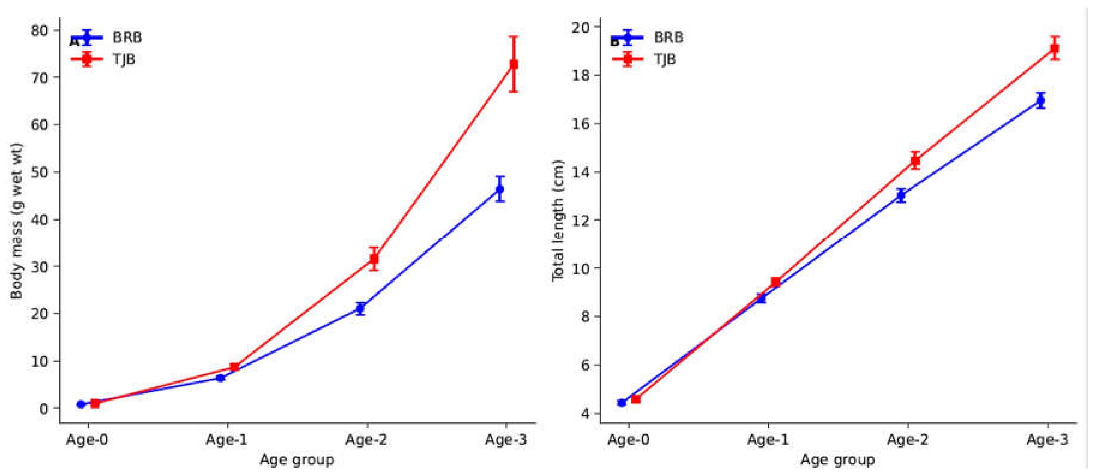
Figure 2.
Relationships between growth performance of age 0+ brown trout and total brown trout density (0+–4+ per 100 m2) in BRB and TJB. Shaded areas indicate 95% confidence intervals around the fitted relationships.
Figure 2.
Relationships between growth performance of age 0+ brown trout and total brown trout density (0+–4+ per 100 m2) in BRB and TJB. Shaded areas indicate 95% confidence intervals around the fitted relationships.
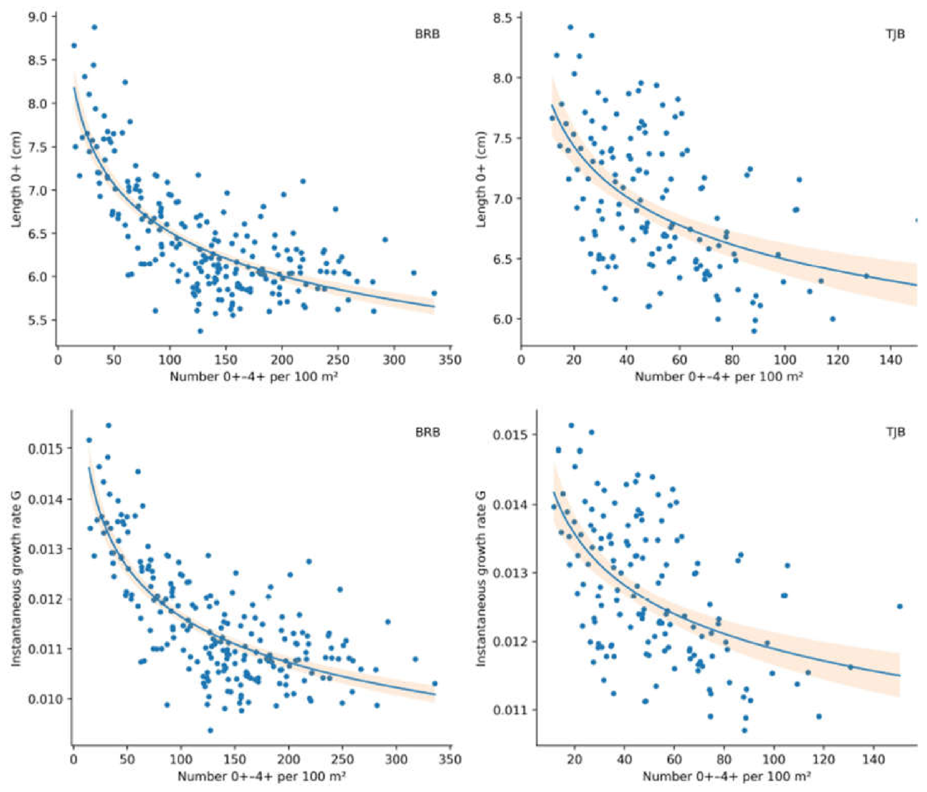
Figure 3.
Relationships between the coefficient of variation of age-0+ trout (CV% age 0+) and (panel A) length of 0+ trout and (B) density (number of 0+–4+ trout per 100 m2) in BRB and TJB. Lines show power functions fitted in log–log space and back-transformed to the original scale. Shaded areas indicate 95% confidence intervals.
Figure 3.
Relationships between the coefficient of variation of age-0+ trout (CV% age 0+) and (panel A) length of 0+ trout and (B) density (number of 0+–4+ trout per 100 m2) in BRB and TJB. Lines show power functions fitted in log–log space and back-transformed to the original scale. Shaded areas indicate 95% confidence intervals.
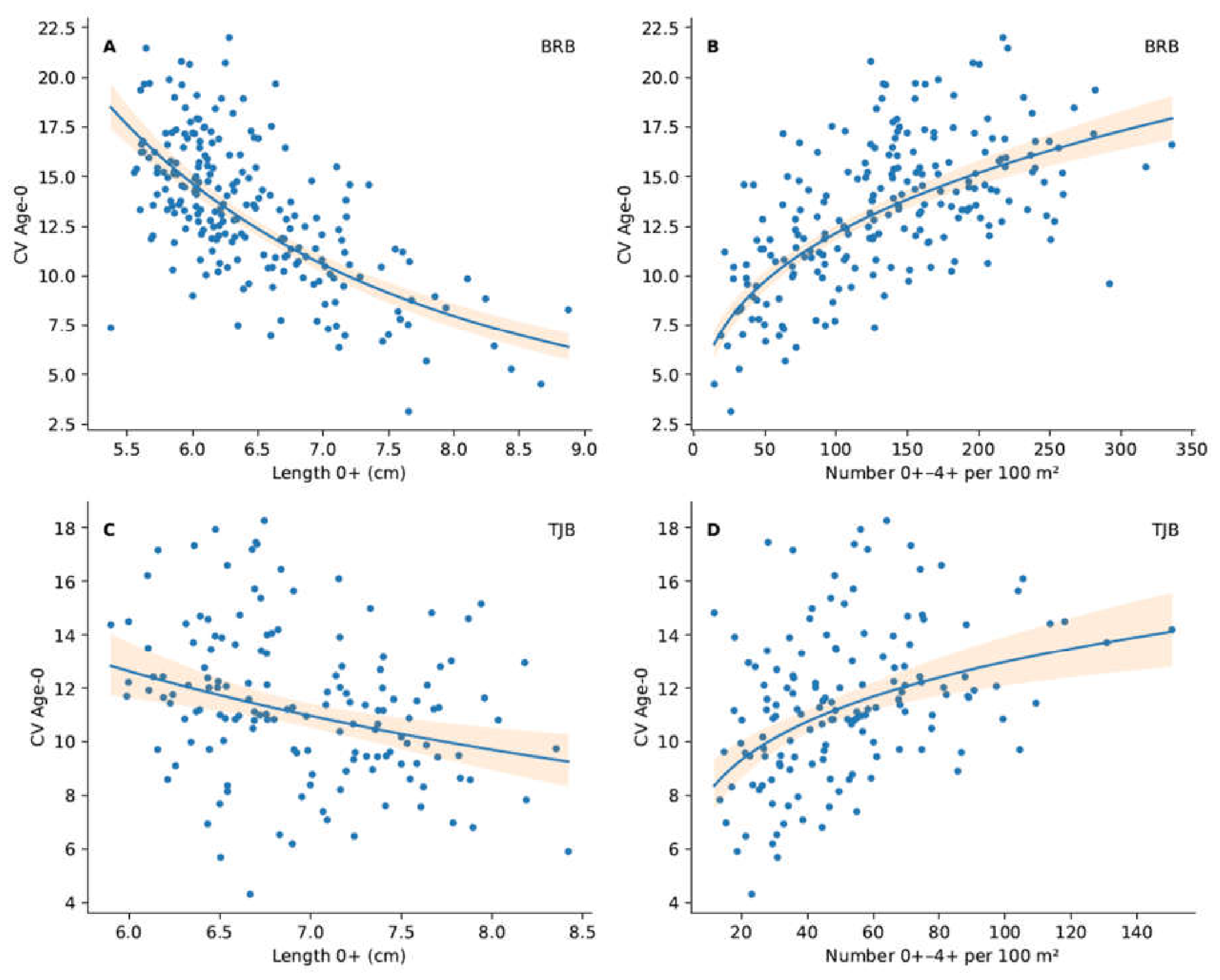
Figure 4.
Relationship between number of recruits and total cohort production (panel a) and production per recruit (panel b) in BRB, TJB and KJB. Points represent cohort observations. Lines show fitted model predictions, and shaded areas represent 95% confidence intervals. Panel (a) is based on a logarithmic regression, whereas panel (b) is based on a power-function model fitted on log-transformed data.
Figure 4.
Relationship between number of recruits and total cohort production (panel a) and production per recruit (panel b) in BRB, TJB and KJB. Points represent cohort observations. Lines show fitted model predictions, and shaded areas represent 95% confidence intervals. Panel (a) is based on a logarithmic regression, whereas panel (b) is based on a power-function model fitted on log-transformed data.
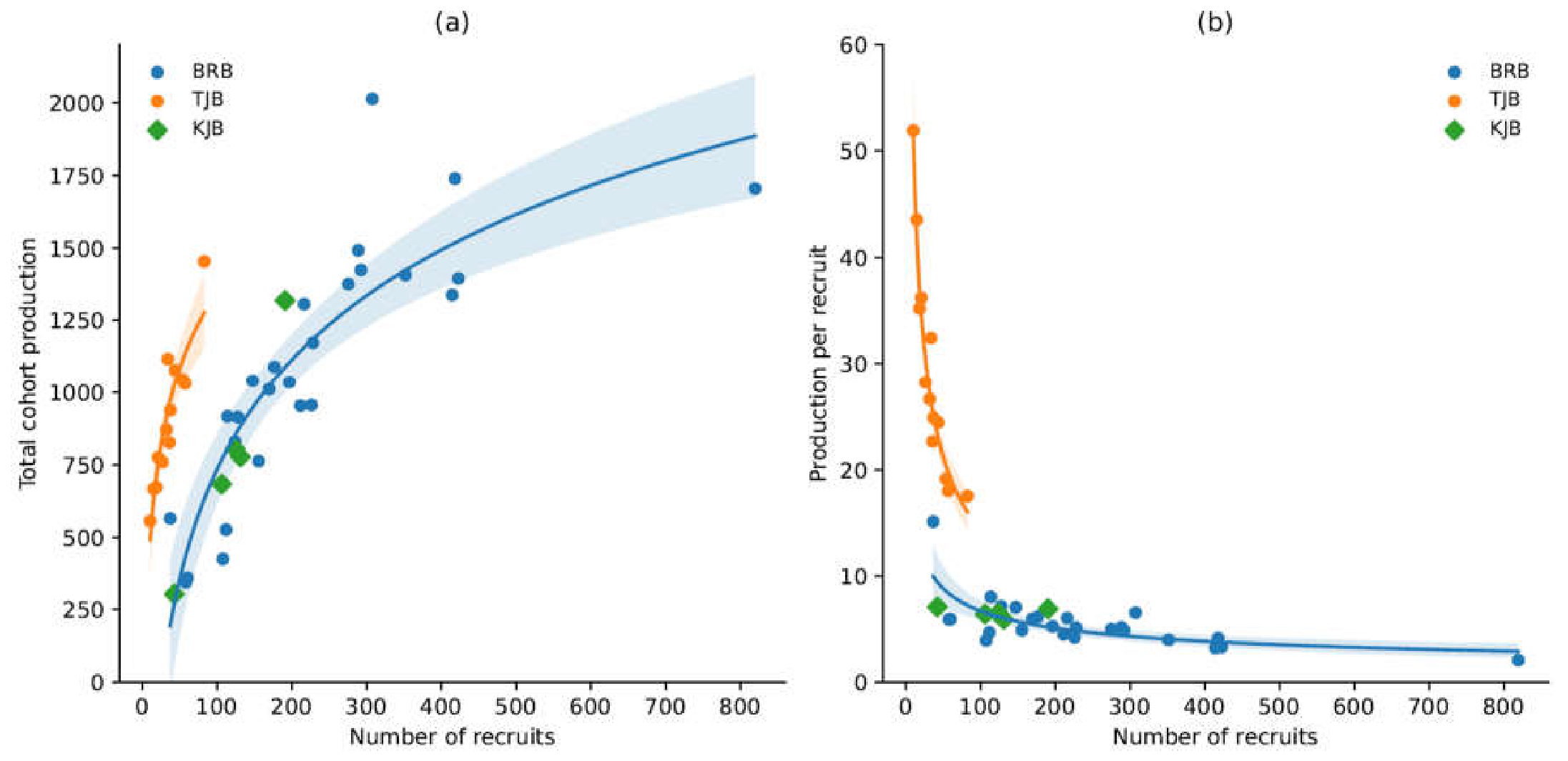
Figure 5.
Temporal variation in yearly production of brown trout in BRB and TJB.
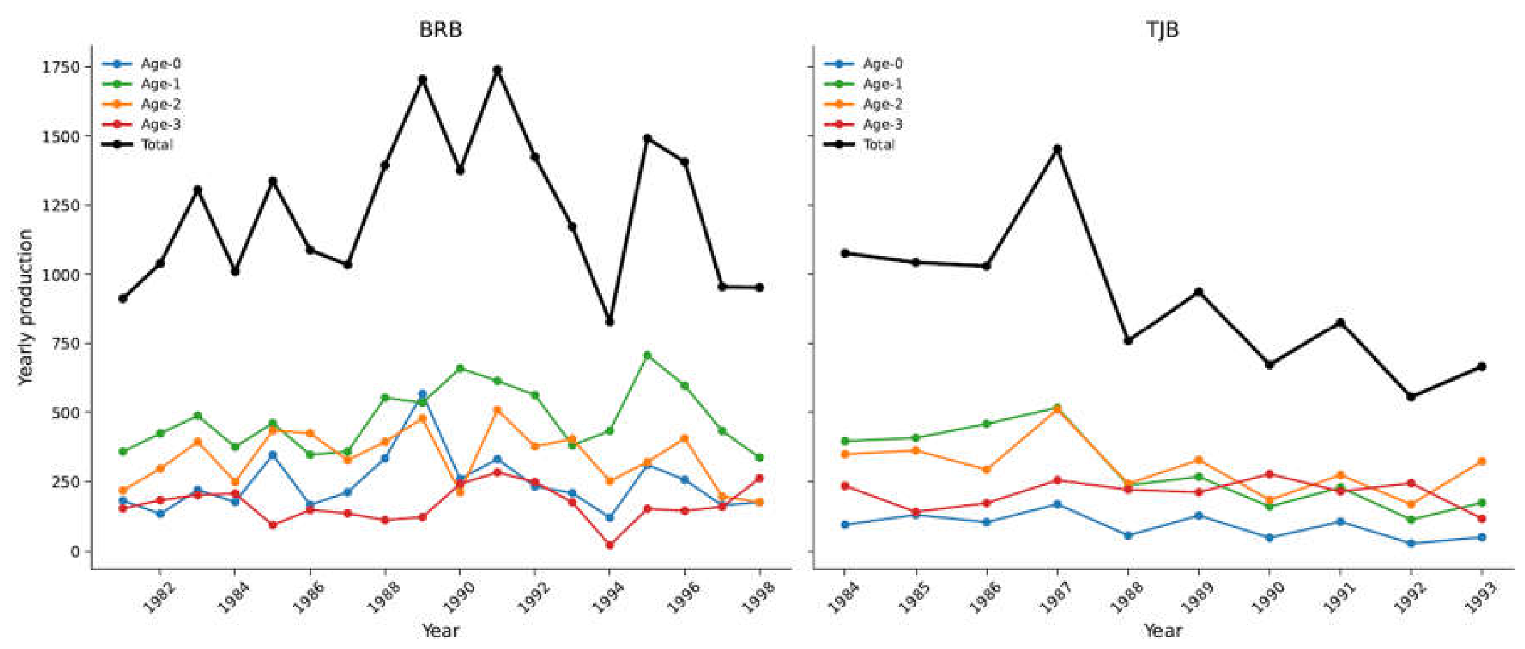
Figure 6.
Relationship between number of recruits and total cohort consumption (panel a) and consumption per recruit (panel b) in BRB and TJB. Points represent yearly observations. Lines show fitted model predictions, and shaded areas represent 95% confidence intervals. Panel (a) is based on a logarithmic regression, whereas panel (b) is based on a power-function model fitted on log-transformed data.
Figure 6.
Relationship between number of recruits and total cohort consumption (panel a) and consumption per recruit (panel b) in BRB and TJB. Points represent yearly observations. Lines show fitted model predictions, and shaded areas represent 95% confidence intervals. Panel (a) is based on a logarithmic regression, whereas panel (b) is based on a power-function model fitted on log-transformed data.
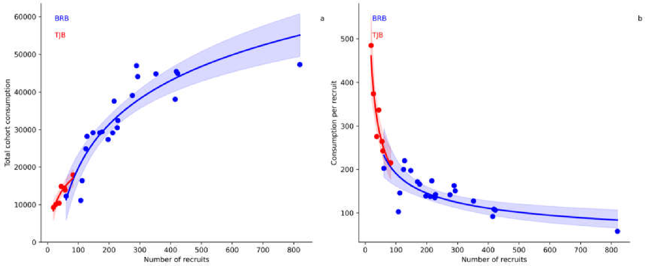
Figure 7.
Temporal variation in yearly consumption (g wet wt.) of brown trout year classes in BRB and TJB. Yearly consumption (per 100 m2) of brown trout year classes in BRB (panel a) and TJB (panel b). Separate curves are shown for Age-0, Age-1, Age-2, Age-3, and total yearly consumption summed across all year classes. The black curve represents total yearly consumption, whereas coloured curves represent year class-specific consumption.
Figure 7.
Temporal variation in yearly consumption (g wet wt.) of brown trout year classes in BRB and TJB. Yearly consumption (per 100 m2) of brown trout year classes in BRB (panel a) and TJB (panel b). Separate curves are shown for Age-0, Age-1, Age-2, Age-3, and total yearly consumption summed across all year classes. The black curve represents total yearly consumption, whereas coloured curves represent year class-specific consumption.
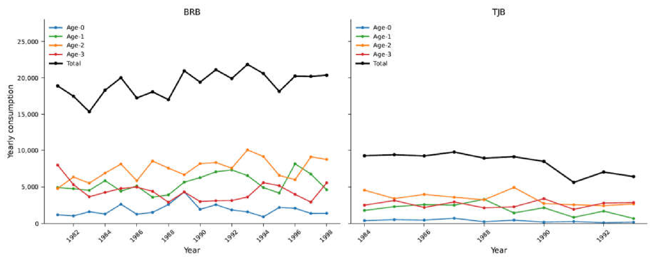
Figure 8.
Relationships between the energetic production-to-consumption ratio (P/C) and (panel A) the number of recruits (N), and (panel B) body mass (g wet wt.) of brown trout in BRB and TJB. Points represent yearly observations. In panel A, fitted curves show the relationship between energetic P/C and recruit abundance, with shaded areas indicating 95% confidence intervals. In panel B, symbols represent different age groups (Age-0 to Age-3) and fitted power functions describe the decline in energetic P/C with increasing body mass. The energetic P/C ratio represents the efficiency by which consumed energy is converted into fish production.
Figure 8.
Relationships between the energetic production-to-consumption ratio (P/C) and (panel A) the number of recruits (N), and (panel B) body mass (g wet wt.) of brown trout in BRB and TJB. Points represent yearly observations. In panel A, fitted curves show the relationship between energetic P/C and recruit abundance, with shaded areas indicating 95% confidence intervals. In panel B, symbols represent different age groups (Age-0 to Age-3) and fitted power functions describe the decline in energetic P/C with increasing body mass. The energetic P/C ratio represents the efficiency by which consumed energy is converted into fish production.
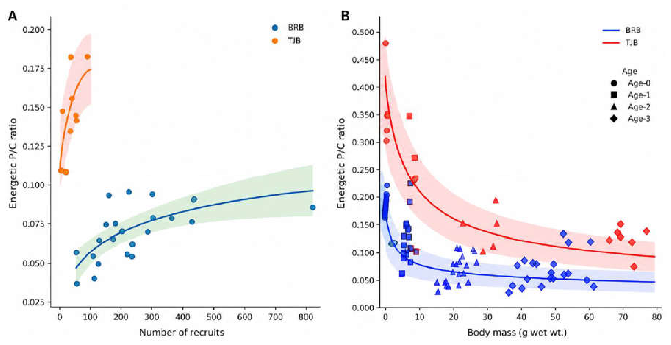
Figure 9.
Relationships between natural instantaneous mortality (M) of age-0 brown trout and (panel a) total population density (Age-0 to Age-3), (panel b) total consumption (Age-0 to Age-3), and (panel c) body mass of Age-0 individuals. Points represent annual observations in TJB (red) and BRB (blue). Solid lines show fitted linear models with a common slope across localities, and shaded areas represent 95% confidence intervals.
Figure 9.
Relationships between natural instantaneous mortality (M) of age-0 brown trout and (panel a) total population density (Age-0 to Age-3), (panel b) total consumption (Age-0 to Age-3), and (panel c) body mass of Age-0 individuals. Points represent annual observations in TJB (red) and BRB (blue). Solid lines show fitted linear models with a common slope across localities, and shaded areas represent 95% confidence intervals.
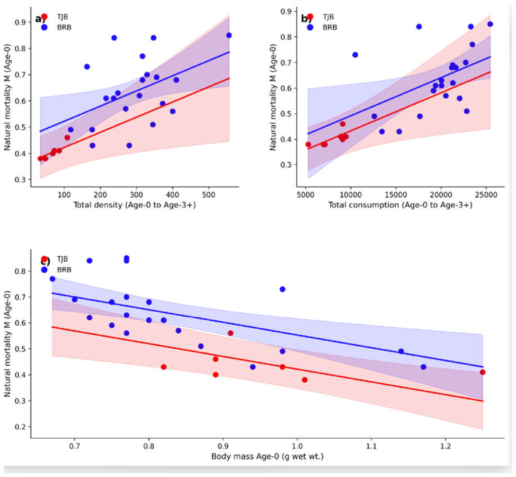

Table 1.
Diet composition of brown trout. Diet composition expressed as mean number of prey items per fish. NoC (%) = percentage occurrence in stomachs containing food. Rare taxa indicated by x.
Table 1.
Diet composition of brown trout. Diet composition expressed as mean number of prey items per fish. NoC (%) = percentage occurrence in stomachs containing food. Rare taxa indicated by x.
| BRB | ||||||||||||||||
| Taxa | 6 Feb. | 9 Apr. | 3 May | 2 Aug. | 6 Nov. | Feb.–Nov. | NoC % | |||||||||
| No. trout | 37 | 32 | 16 | 34 | 35 | 154 | ||||||||||
| Length | 5.2–19.0 | 9.9–19.0 | 10.6–19.3 | 4.9–20.6 | 4.9–20.9 | 4.9–20.9 | ||||||||||
| Empty % | 10.8 | 6.3 | 0.0 | 0.0 | 2.9 | 4.5 | ||||||||||
| Asellus | – | x | – | – | x | – | – | |||||||||
| Gammarus | – | 2.5 | 4.3 | 2.0 | 1.0 | 3.0 | 10.9 | |||||||||
| Ephemeroptera nymph | – | 4.6 | 4.3 | 3.5 | 4.0 | 4.0 | 21.8 | |||||||||
| Plecoptera nymph | 1.0 | 7.1 | 2.8 | 1.4 | 2.3 | 2.3 | 40.1 | |||||||||
| Tricoptera larvae | – | 5.0 | 3.6 | 1.9 | 7.0 | 4.5 | 68.7 | |||||||||
| Chironomidae larvae | 1.0 | 7.4 | 2.6 | 5.1 | 5.4 | 5.1 | 50.3 | |||||||||
| Diptera & Simuliidae | 1.0 | 1.6 | 1.3 | 3.1 | 1.7 | 2.0 | 25.9 | |||||||||
| Coleoptera larvae | 1.0 | 1.6 | 4.0 | 2.4 | 1.3 | 2.1 | 21.1 | |||||||||
| Lepidoptera larvae | x | |||||||||||||||
| Neuroptera nymph | x | x | ||||||||||||||
| Dermaptera | x | |||||||||||||||
| Odonata nymph | x | |||||||||||||||
| Heteroptera | x | |||||||||||||||
| Hymenoptera adult | x | x | ||||||||||||||
| Arachnida | x | |||||||||||||||
| Diplopoda | x | x | x | |||||||||||||
| Gastropoda | x | |||||||||||||||
| Lumbricidae | x | x | x | x | ||||||||||||
| Lamprey | x | |||||||||||||||
| S. trutta egg | x | x | ||||||||||||||
| TJB | ||||||||||||||||
| Taxa | 6 Apr. | 8 Jun. | 8 Jul. | 26 Aug. | 20 Sep. | 12 Oct. | 14 Dec. | Apr.–Dec. | NoC % | |||||||
| No. trout | 18 | 11 | 19 | 21 | 4 | 22 | 24 | 119 | ||||||||
| Length | 7.4–11.5 | 7.6–10.5 | 4–11.8 | 4.8–13.9 | 5.6–7 | 5–17.1 | 5–15 | 4–17.1 | ||||||||
| Empty % | 5.6 | 0 | 5.3 | 0 | 0 | 0 | 0 | 1.7 | ||||||||
| Asellus | – | – | 0.1 | 0.6 | 0.3 | 0.1 | 0.1 | 0.2 | 11.1 | |||||||
| Gammarus | 0.6 | 0.2 | 0.2 | 1.4 | 0.3 | 0.3 | 0.5 | 0.6 | 30.8 | |||||||
| Ephemeroptera nymph | 2.1 | 2.5 | 1.8 | 0.2 | – | 1.3 | 1.8 | 1.8 | 59.0 | |||||||
| Plecoptera nymph | – | – | – | – | x | – | – | – | – | |||||||
| Tricoptera larvae | 1.4 | 0.5 | 1.2 | 1.0 | – | 0.8 | 0.3 | 0.9 | 45.3 | |||||||
| Chironomidae larvae | 2.5 | 0.2 | 0.6 | 6.9 | 0.8 | 5.8 | 5.6 | 4.0 | 53.8 | |||||||
| Diptera & Simuliidae | 0.2 | – | 0.1 | 0.4 | – | – | – | 0.1 | 20.5 | |||||||
| Coleoptera larvae | 0.2 | 0.9 | 0.2 | – | – | 0.4 | – | 0.4 | 17.1 | |||||||
| Lepidoptera larvae | x | x | ||||||||||||||
| Heteroptera | x | x | x | |||||||||||||
| Arachnida | x | x | x | |||||||||||||
| Gastropoda | x | x | ||||||||||||||
| Lumbricidae | x | x | x | x | ||||||||||||
Disclaimer/Publisher’s Note: The statements, opinions and data contained in all publications are solely those of the individual author(s) and contributor(s) and not of MDPI and/or the editor(s). MDPI and/or the editor(s) disclaim responsibility for any injury to people or property resulting from any ideas, methods, instructions or products referred to in the content. |
© 2026 by the authors. Licensee MDPI, Basel, Switzerland. This article is an open access article distributed under the terms and conditions of the Creative Commons Attribution (CC BY) license (http://creativecommons.org/licenses/by/4.0/).
Copyright: This open access article is published under a Creative Commons CC BY 4.0 license, which permit the free download, distribution, and reuse, provided that the author and preprint are cited in any reuse.


