
Submitted:
16 July 2026
Posted:
17 July 2026
You are already at the latest version
Abstract
In light of strong expansion of renewables, electrolysis may act as an alternative to conventional grid enforcement to overcome grid constraints in a timely and effective manner as it creates additional flexible load and thus enables renewable production peaks to be absorbed. This paper examines whether hydrogen electrolysis can serve as a cost-effective alternative to conventional grid reinforcement in Austrian electricity distribution networks. It goes beyond the current state of art by using three real-world case studies in Styria, using an integrated techno-economic framework combining distribution-grid simulations, market optimization, PEM electrolysis modelling and cost-benefit analysis to compare the grid-supportive electrolysis against conventional grid enforcement. The results demonstrate that grid-supportive electrolysis can become competitive under suitable hydrogen market conditions. When operated in grid-supportive mode only, the capacity factor for the electrolysis lies below 5%. Economic viability emerges only when electrolysers are allowed to combine grid-supportive operation with market-driven hydrogen production. Thereby, the hydrogen price proves to be the key determinant: a hydrogen price above approximately 6 EUR/kg incentivizes market based operation and naturally resolves grid congestion without further intervention by the DSO. In some locations, smaller electrolysers (around 20–60% of the theoretically required size) deliver the best economic performance, recovering most curtailed renewable energy while limiting investment costs compared to conventional grid extension.
Keywords:
electrolysis
; distribution grid
; hydrogen
; grid-supportive operation
1. Introduction
The European Green Deal aims to achieve climate neutrality by 2050 and 55 % reduction of emissions by 2030. Austria is even more ambitious and has set the goal of covering 100 % of electricity demand via renewable sources by 2030 [1] and achieving climate neutrality by 2040. To achieve these goals, rapid deployment of intermittent renewable energy sources (RES) is required and to overcome the temporal and geographical mismatch between demand and intermittent supply, significant electricity grid expansion and enforcement measures are required. Some estimations quantify the expenditures to around 24 billion euros by 2030 for the distribution grid [2] and 9 billion euros for the transmission grid by 2035 [3].
Alternatively, the geographical and temporal gap could be solved through flexibility or the deployment of electrolysis specifically. In this respect, electrolysis could create additional value in many different aspects: Enabled by the fast reaction time of proton exchange membrane electrolyzers (PEMEL) [4,5] it would cover the need for flexibility, avoid lengthy grid-enforcement measures and also ensure energy resilience by enabling local hydrogen production [6]. Within the European Green deal, electrolysis capacity of 40 GW is envisaged by 2030, of which 1 GW should be located in Austria [7]. In this sense, electrolysis as a flexibility option would create strong synergies.
From a scientific point of view, a research gap exists since it is unclear whether electrolysis can act as a cost-efficient measure to overcome congestion in the distribution grid in a techno-economic sense. Most of the existing studies focus on slightly different aspects, for example the economics of electrolysis by providing balancing services, the physical aspects, e.g., the impact of electrolysis on grid congestion, or the benefits of additional load from electrolysis for the integration of renewables into the grid. In contrast to that, our work uniquely combines a detailed grid simulation, market optimisation, technical modelling of the electrolyzer with a cost-benefit analysis to evaluate the economics against conventional grid extension and find the optimal capacity of the electrolysis in a techno-economic sense, based on three real-world case studies. This provides a valuable contribution to the research field, specifically with respect to the explicit comparison against conventional grid reinforcement, the economically optimal sizing of the electrolysis and the combination of various methods into an integrated approach.
1.1. Aim and Outline
The main contribution of this work is an integrated assessment combining grid simulation, market optimisation, technical modelling of the electrolyser and cost-benefit analysis. Previous studies mostly investigate specific parts, but an integrated approach could indeed not be identified. Another novelty consists in the comparison of the electrolysis in distribution grids to conventional grid enforcement measures. This is done on the basis of three case studies in the network area of the distribution system operator (DSO) ‘Energienetze Steiermark’, which improves generalisability compared to synthetic networks. Detailed distribution grid simulation is undertaken in PowerFactory (described in Section 2.2) to model the actual power flows, identify overloaded network components, determine the electrolyzer nominal power and minimal grid-supportive behavior to avoid curtailment of renewable energy sources (RES). In a next step, the market based operation (described in Section 2.3) is determined through optimal behavior of the electrolysis against historical electricity prices and hypothetical prices for hydrogen. A technical simulation (described in Section 2.4) then assures a correct representation of non-linear efficiencies and minimum-stable generation of the electrolysis. Finally, the results are evaluated in a cost-benefit analysis (CBA, as described in Section 2.5) and compared against the cost of conventional grid expansion.
Resolving grid-congestions through electrolysis lies precisely on the intersection between market and electricity-network operation. By European law ([8]) article 36, grid operators are, broadly speaking, not allowed to own and operate storages or generation assets. In Austria specifically, according to § 72 and 73 ElWG [9], DSOs are basically ruled out from owning and/or operating storage facilities. There are very few exemptions, but these exemptions allow for grid-supportive operation only, as elaborated by [10]. Therefore, the integration of grid-supportive flexibilities into the network requires the development of feasible organisational models. The focus of this work is on techno-economic results, but some regulatory aspects are discussed at the very end of the paper to emphasize the importance of the organisational implementation.
1.2. Literature Review
There are a number of studies that investigate the operation of electrolysis in relation to the electricity grid. Some of them focus on ancillary services, from a technical and economic perspective. Within the H2Future project [11], a use-case for the installed demo plant (6 MW) was to test the suitability of the PEMEL system to participate on the balancing markets by the provision of system services and [12] investigated the potential of Pressurized Alkaline Electrolyzer technology for the provision of grid services based on the assessment of a 3.2 MW demo plant. [13] looks at the provision of primary balancing reserve in Belgium by 25 MW electrolyzer. In [4], power hardware in the loop tests of a 225 kW proton exchange membrane electrolyzer (PEMEL) were conducted. The goal of this study was to provide slow voltage control but also fast frequency control for an emulated distribution grid at 0, 25 and 50 % RES penetration. It was concluded, that both approaches are technically feasible without meaningful restrictions to the summative hydrogen production. This was possible as the base power was set to 50 % of the nominal power of the PEMEL and positive and negative deviations canceled each other. This technical limitation of this approach reduces the capacity factor of the PEMEL and could possibly reduce its economical viability. The interaction between the energy system and PEM electrolysis is studied in [14] by conducting a life cycle assessment by considering the CO2-footprint of the future electricity system in Germany.
The interaction of electrolysis with the electricity grid is investigated in some studies, mostly from a technical point of view. For example, the study [15] investigates, whether decentralised electrolysis can play a vital role for the intregration of renewables. The study works with synthetic electricity networks for five different locations in Germany and finds that small decentralised electrolyzers with size below 5 MW can play a central role to support the local distribution grid and absorb excess renewable feedin. In a similar manner, [16] look at the interaction between high-voltage grid and alkaline water electrolysis in Germany using linear power flow optimisation with PyPSA and open source grid-data. They find that electrolysis capacities above 300 MW are required to cause supra-regional impacts. While this study models precisely the dynamics behind the transmission grid and the electrolyzer, no economic analysis is undertaken. The work of [17], discusses the advantages and disadvantages of grid-supportive flexible electrolysis operation on a qualitative basis for Germany. For example, in the work of [18], the concept of hydrogen supply chains in the context of electricity distribution grids is analyzed in the literature through a text-mining approach and finds that hydrogen production is not yet linked to solving problems arising in the electricity network.
While previous studies mostly focused on the impact on the grid, there is also a variation of studies showing the economic viability of PEMEL when providing ancillary services. In [19], a techno-economic valuation of electrolysis in regard to the provision of balancing energy is undertaken. The work basically concludes that revenues from balancing services are not sufficiently attractive for an electrolyzer to be profitable. This aligns with the conclusion of this work that multiple revenue streams (or high incentives from the hydrogen market) are required to make electrolysis economicially viable. To reduce the risk of unmet demand by such energy-intensive reserves (as stated in [4]), [20] showed that flexible bidding for control reserve can mitigate these risks while maintaining profitability. While our work focuses on electrolysis being installed to avoid overloading of grid components, one could also look at the opposite direction and check, whether electrolysis causes grid congestion on the other hand. For example, the work of [21] finds that the integration of hydrogen under the current pricing scheme may lead to higher congestion costs in Germany. This finding is valid for the transmission grid with purely market based behaviour while our study focuses on the distribution grid and explicitly requires a grid-supportive behaviour.
2. Methods and Data
The techno-economic modelling is structured in four main steps: (1) grid simulation, (2) market optimisation, (3) technical PEM modelling, (4) cost-benefit analysis. First, the grid is simulated with PowerFactory to determine the grid-supportive behavior and the size of the power to gas (P2G) system. Second, market based operation then maximizes profits based on market signals. The result of the market optimisation is corrected by the constraints of the technical simulation, to determine the technically correct operation considering non-linear efficiencies, minimum stable load of the electrolyzer system and minimum grid-supportive behaviour. In a last step, based on the simulation results of the technical simulation model, a cost-benefit-analysis is undertaken to account for costs and revenues resulting from ownership and operation of the electrolyzer and compare the results against conventional grid extension. The interplay and interdependencies of these steps are illustrated in Figure 1.
2.1. Simulation Approach
Three promising locations for grid-supporting electrolysis in the distribution grid of ‘Energienetze Steiermark’ (located in Styria, Austria) are considered. Figure 2 illustrates the network area of ‘Energienetze Steiermark’, in line with the plans of the H2 Roadmap [22] and the European Hydrogen Backbone (EHB) [23]. Within this network area, three locations were selected. For confidentiality reasons from side of the DSO, the exact location of the three P2G systems cannot not be disclosed, but for electrolysis to make sense as a substitute to conventional grid-enforcement measures, potential locations need to fulfill a number of requirements. First and most obvious, grid-bottlenecks caused by future infeed and limitation of current grid capacity are expected and need to be solved. Second, and this is probably related to the first condition, these locations will be close to areas with high expected deployment of intermittent renewable generation. Third, proximity to the future hydrogen network is considered to be essential as a sink for the produced hydrogen. Put differently, electrolysis will be positioned at the intersection of i) high-voltage electricity grid, ii) envisaged RES build and iii) the envisaged hydrogen network. In these three selected locations, the surrounding grid was modelled and the P2G systems were positioned.
The overall simulation is carried out for a timeframe of 30 years (2025-2055) to show the increasing need of grid reinforcement due to increasing implementation of RES generation (mostly PV, but also wind), while also considering increasing electricity demand (private EV and private heat pump rollout scenarios where considered). To represent a discrete expansion of P2G capacity to counteract grid congestion by increasing feed-in, a five-year expansion cycle was implemented. In the beginning of each five-year simulation cycle, the maximum grid congestion was taken as reference for expansion capacity of the upcoming five years.
The modelling was undertaken against historical data of 2023 with respect to RES generation and load profiles, electricity prices and grid charges. Strong expansion of RES was assumed in accordance with [1,24], as further outlined in Section 2.2. Despite some efforts to predict and estimate future prices or costs of hydrogen (see for example [25,26,27]), we consider the hydrogen price as the most uncertain variable in this modelling exercise. Therefore, the hydrogen price is exogenously given and varied in a range between 1 and 10 EUR/kg.1 In all locations, it is assumed that the P2G is grid-connected (front of meter) and is not working co-located being directly connected to the plant (behind the meter). This implies that grid charges are applicable to their full extent.
2.2. Grid Simulation
As a first step, a grid simulation was undertaken to determine the grid-supportive operation. The grid-supportive operation was defined as the minimal required operation of the electrolyzer, to compensate peaks of renewables production which would have led to violation of grid constraints and as a consequence of infeed curtailment. It is a rule-based strategy and is determined on the basis of grid simulation and the respective technical limits of network components.
This is said to be the minimal required operation of the P2G to consume renewable generation and thus maintain valid operational state of the grid. Hence, the P2G is designed in order to compensate the maximum grid-violation that can be observed within the modelled timeframe. On the other hand, the P2G load is constrained from the upper side the grid is overloaded from the demand side. This typically happens when renewable infeed is low or zero and consumption is high. Considering both limitations from the upper and lower side, the P2G is left with an operational window, reflecting the minimum load required to absorb production peaks and constraints from the upper side reflecting demand peaks.
Figure 3 depicts such an operational window in a simplified way by meeting primary substation capacity limit as an example of a bottleneck of a distribution grid. In this example, grid components would be overloaded from excess feed-in between 9:00 and 17:00. The maximum overload is 10 MW at 13:00. Therefore, the P2G is designed at a capacity of 10 MW. However, when running at full capacity, it would lead to a congestion between hour 2 and 7 as well as 19 and 23, hence, the operational window is reduced during these timeframes by the required amount. Typical bottlenecks of distribution grids are line loading limits (predominantly in network level 3), primary substation capacity (predominantly for network level 4 – see Figure 3), or grid voltage limits (predominantly network level 5).
The grid simulation was built in Digsilent PowerFactory2 and the whole calculation was automatized by the PowerFactory Python interface, so future scenarios and controls where setup using Python, and PowerFactory was fully controlled via Python. For yearly simulation, yearly consumption and generation profiles were configured in the grid, and the PowerFactory Quasi-Dynamic-Simulation function was used to calculate one year within 15 min timesteps with high performance. Yearly consumption and generation profiles were provided by the DSO, containing real measurement data from primary substation transformers and feeders in the historical timeframe from 2023-01-01 to 2023-12-31 in 15-minutes granularity.
Figure 4 shows the grid topology of all three locations. All three locations are characterized by different grid layouts and therefore, the P2G is connected at different network levels spanning from network level 3 to network level 5. Figure 5 illustrates the assumptions on RES expansion and Figure 6 depicts the assumptions for growth of demand due to electrification of heat and mobility in all three locations. Location A and Location C are characterised by low-voltage (LV) and medium-voltage (MV) photovoltaic rollout, while Location B experiences also some increase in wind capacities. The assumptions are based on multiple sources, e.g., [28,29] and were fine-tuned based on several discussions with the DSO, being aware of the local conditions. In all locations, significant expansion of RES as well as additional demand from heatpumps and electric vehicles (EVs) is expected.
Location A
The P2G is supposed to relieve the substation on network level 4. The current demand/injection (historical data 2023) spans between +9 MW (demand) and -17 MW (injection). The transformer station capacity (considering n-1 security) lies between +50 MW and -100 MW. Strong growth of solar PV on low voltage (LV) and medium voltage (LV) is assumed.
Location B
The P2G is supposed to relieve a grid branch on 110 kV level (network level 3). The current demand/injection spans between +50 MW and -15 MW. The line capacities are between +100 MVA and -200 MVA for “lower” line and +200 and -400 MVA for “upper” line. Strong growth of wind and solar PV is anticipated.
Location C
One feeder of a 20 kV medium voltage (MV) grid is modelled that is characterized by two main branches. Current peak load in this feeder is around 2.3 MW and maximal RES generation at minimal load causes a reverse power flow -0.63 MW. To increase hosting capacity to enable the expected amount of PV integration, one P2G was located in each of the branches on network level 5. While one of the branches is around 19 km long and the other around 22 km, the P2G were placed on the most optimal location in the feeder to compensate future PV infeed most effectively. According to current common practice in network planning, network level 5 consumers are not allowed to consume more than 8 to max. 10 MW, which constitutes a non-technical limit for the size of the P2G.
2.3. Market Based Operation
The optimal operation based on market signals is determined by solving an optimization problem, implemented in the IESopt framework [30]. IESopt is an open-source optimization framework built on top of the JuMP modeling language [31], written in Julia [32] with a Python interface.
For the market based operation, the P2G system is modelled as a price taker against the electricity market. The optimal market based operation is a result of the marginal costs of hydrogen production and the hydrogen price. While the hydrogen price is assumed to be exogenous, the marginal costs of hydrogen production is determined by the electricity price, the grid charges and the conversion ratio of the P2G. For the electricity price, quarter-hourly historical spot market prices for Austria in the year 2023 are considered. The grid charges are taken from historical data for the network area of Styria and consist of an energy component in EUR/MWh and a peak-load component in EUR/MW for the monthly quarter-hourly consumption peak, as described in Table 1. The optimization maximizes yearly profits by choosing electricity consumption of the P2G, being constrained by the size of the P2G and facing electricity prices and grid charges as costs. The output value of the P2G is determined by the exogenously assumed hydrogen price.
The modeling assumes perfect foresight on the electricity prices over one entire month, because peak-load grid charges are settled monthly in Austria. Hence, market based operation is determined month-ahead on a quarter-hourly resolution. Since the market based operation is implemented as linear program (LP), the conversion ratio of the P2G as produced hydrogen mass per electric input is considered at a constant value of ~18.3 kg/MWh. The optimization always chooses full load as long as the marginal costs of production fall below the hydrogen price, considering fixed costs arising from peak load grid charges. Therefore, no minimum load arising from the technical specifications of PEMEL is considered in the optimization model.
The monthly operation schedule determined by the optimization model is then used as in input in the technical simulation model. The technical simulation combines the operational schedules of the grid simulation and the market based operation. The technical simulation makes sure that the operational schedule of the P2G lies within the operational window, as illustrated in Section 3. In addition, the technical simulation model considers the non-linearities and varying conversion factors as a function of load, which provides a preciser inputs to the cost-benefit analysis when the P2G is working in partial load. This is particularly the case when the P2G is working in grid-supportive mode only or the market based operation is limited from the upper side due to grid constraints.
2.4. Technical Simulation
The technical simulation corrects the results of the market optimisation and aims to adequately reflect the technical characteristics of the P2G. To properly absorb renewable production peaks, the selected electrolysis technology must be appropriately flexible. Therefore, due to its higher flexibility in dealing with power ramping, PEM technology was chosen for the electrolyzer [33,34]. To represent the technical lifetime of the PEMEL, it is assumed that after end of life, the electrolyzer must be removed or replaced. Regarding lifetime, literature diverges quite extremely by giving values of 20,000 to 90,000 hours of operation or 10 to 25 years [14,35,36,37]. Therefore, a lump-sum lifetime of 15 years was assumed, even though it might seem a little overestimated for a possible full load operation (e.g., a total lifetime of 90,000 hours leads to a capacity factor of around 0.68 for a lifetime of 15 years). Assuming a lifetime of 15 years when considering a timeframe between 2025 and 2055 implies reinvestment around 2040. Reinvestment is then evaluated at the relevant CAPEX value of the respective year.
The system simulated in this study is designed to provide a realistic representation of a P2G system. Starting at the coupling point to the electrical distribution grid, alternating current is converted into direct current using an ACDC converter. For location B, an additional transformer is needed at the substation due to technical specifications.3 Direct current is fed into the PEMEL. The output of the electrolyzer would normally be buffered in a small-scale hydrogen storage tank (with a storage time of about two hours based on the electrolyzer output) to ensure a constant or quasi-constant back pressure to the hydrogen output stream of the electrolyzer. Due to the limited losses of the storage tank and its small size, which makes it only usable for technical purposes, it is neglected in the simulated system. The compressor required to increase the pressure of the hydrogen gas before feeding it into the pipeline is assigned to the gas grid. The compressor therefore has no influence on the P2G in technical or economic terms and is also neglected.
The technical modelling is carried out using TESCA, an internal AIT framework for deterministic time series simulations [38]. The simulation framework provides models for various components of energy systems in the electricity, hydrogen and heat sectors. For this study, the electricity and hydrogen grids were implemented as unlimited source and unlimited sink, respectively. Therefore, the P2G system was only restricted by its own technical boundaries, like nominal power of the components. The transformer and the ACDC converter were implemented with load-dependent efficiency curves.
In contrast to the models of transformer and ACDC converter, integration of the core component of the P2G, the PEMEL, into the entire system is based on in-depth modeling of the electrochemical process from [39]. The efficiency of electrolysis is calculated as a combination of voltage efficiency and faraday efficiency . Voltage efficiency on the one hand accounts for electric losses in the PEM cell. It is computed as outlined in (1), where thermoneutral voltage is and total cell voltage as defined in (2).
The reversible voltage depends on both the operational temperature and pressure, and activation overpotentials of anode and cathode accounting for kinetics at the electrodes, and ohmic overvoltage accounting for ohmic losses in the membrane. As activation overpotentials increase with the natural logarithm of the applied current and ohmic losses linearly to the applied current, voltage losses are increasing for increasing applied electrical power. Faraday efficiency on the other hand accounts for back-diffusion of hydrogen through the membrane by the pressure difference, reducing the actual hydrogen throughput of the electrolyzer. Hydrogen back-diffusion is not depending on the theoretical throughput, but rather on the pressure difference between cathode and anode side (which are assumed constant as 30 bar at the cathode and 1 bar at the anode side in this study). With constant hydrogen back-diffusion the faraday efficiency increases to 100 % asymptotically in dependency of the load. For auxiliary technology such as water pumps, water treatment and cooling system, a constant auxiliary power of 5 % of the electrolysis nominal power is assumed, reducing the stack efficiency even further to an overall system efficiency of the electrolysis system . Due to the constant nature ot the balance of plant (BoP) power the influence on the overall system efficiency is decreasing with increasing load of the electrolyzer.
2.5. Cost-Benefit Analysis
A cost-benefit analysis (CBA) is undertaken over the entire simulation time frame (e.g., between 2025 and 2055, 30 years). To evaluate measures of the P2G against conventional grid enforcement, a baseline scenario for the entire time frame is defined. In the baseline scenario, the surplus renewables generation is curtailed so that the network can still be operated in its technical boundaries. Then, both scenarios (classic grid enforcement-scenario and P2G-scenario) can be compared to the baseline scenario. Figure 7 shows the main characteristics of the baseline scenario: curtailed energy in GWh and lost revenues in thousand euros from sales on the electricity market. The curtailed generation is a direct consequence of the renewables expansion in combination with the congested grid components and the lost revenues on the electricity market consist of the product of the curtailed generation and the historical electricity prices 2023.
At this point, it is worth mentioning that the cost-benefit analysis takes a global perspective, without a specific view on the ownership structure of the components. For example, lost revenues on the electricity market concern the owner of the renewable plants, not the DSO or the owner of the electrolyzer. However, in a global cost-benefit analysis, revenues and expenses can be added without specific attribution to actors. The composition of costs and benefits from a global perspective are illustrated in Figure 8. First, it can be concluded that, independently of the hydrogen price, the recovered revenues from renewables generation (that would be curtailed in the baseline scenario) contribute to the overall benefits. Assuming a hydrogen price of zero, no market based operation could be observed, but an (unprofitable) grid-supportive operation would maintain network operation within its limits and ensure that all renewables production could be injected into the grid. The computation of the lost revenues is shown in (3), where represents the curtailed electricity in year y at time t and the corresponding electricity price in the respective time interval t. This calculation is repeated and then summed up for each year y between 2025 and 2055, whereby a discount factor r (assumed at 4% in real terms) is applied. Index t represents all quarterly hours of the year and therefore runs from 1 to 35,040.
However, it is obvious that global costs and benefits depend on the assumed hydrogen price. With an increasing hydrogen price (equivalent to willingness to pay for the output of the P2G), revenues from hydrogen sales increase. This is a result of two sources: first, hydrogen output is evaluated at a higher price and, second, the output of the P2G increases since market based operation finds more profitable hours. At some point, we can observe a ‘break-even hydrogen price’ where benefits start to outweigh the costs. Please note that the curves depicted in Figure 8 are drawn for illustrative purposes only. In fact, both curves are non-linear and proportions are very different.
For each location, costs and revenues are accumulated and discounted over the entire time horizon from 2025 to 2050. Equation (4) represents revenues from hydrogen, where denotes the hydrogen output and h the hydrogen price. Total costs of hydrogen production are illustrated in (5) on the basis of annual costs for hydrogen production in (6). Here, denotes the electrical input energy and the electricity price.
Of course, there are some interdependencies in these equations. Electrical input depends on the hydrogen price h and is determined by optimization (based on a linear relationship between and ) to maximize profits from operation of the electrolyzer. In the technical simulation, is then determined as a (non-linear) function of , considering a number of efficiency-curves. The investment costs in a given future year y () are determined by the electrolyzer capacity multiplied by the specific CAPEX value expressed in EUR/kW illustrated in Table 2. The costs for maintenance in the respective year () are compound by the value of 2 % of CAPEX per year.
In the case modeled here, it is assumed that the P2G is connected to the electricity grid (front of meter), feeds into the hydrogen network and does therefore not consume exclusively renewable electricity. Grid costs (GC) for peak load consumption are illustrated in (7), where denotes the peak consumption (maximum load value) within month m and denotes the peak-load grid tariff. In Austria, they are formed by the average across all monthly peak consumption values. Grid costs for energy consumption are illustrated in (8) which are composed of the total energy consumption multiplied by the variable grid tariff . Specific values for the peak and variable grid tariff are illustrated in Table 1. The data is based on grid costs for Styria [40] and refers to the second amendment in 2023. In this version, reductions were granted from the state to the consumer in light of the energy crises in the sharply rising costs for electricity during 2022. For simplification, we have not assumed grid tariffs for injection.
Electricity prices p consist of historical data for the Day-ahead (15M) EXAA Spot auction from the year 2023 [41] and were kept constant over the entire lifetime. It is clear that this is a strong assumption, however, electricity prices, in particular the upper and the lower end of the price range is notoriously hard to project with long term fundamental models. The average price is around 100 EUR/MWh with prices ranging between 75 EUR/MWh and 130 EUR/MWh in around 50 % of time.
Table 2 illustrates the cost for investment and operation of the PEMEL. Assumptions were taken from the ‘Technology Catalogue for Renewable Fuels’ from the Danish Energy Agency [36]. CAPEX and OPEX assumptions are chosen for a system size around 10 MW. The value is actually applied to higher capacity values between 20-70 MW, but the slightly higher CAPEX due to missing scale-effects should reflect a more conservative approach in light of the fact that CAPEX of electrolysis has been underestimated in the past, see [42]. Actual values for investment in any future year are interpolated from the anchor year values in 2025, 2030 and 2040. For years beyond 2040, the value of 2040 was kept stable.
In a last step, the results of the CBA are compared to the cost of conventional grid enforcement measures. For this purpose, the DSO ‘Energienetze Steiermark’ has estimated the cost of undertaking conventional measures, the values are illustrated in Table 3. These numbers represent the cost of grid enforcement from the point of view in 2023 to ensure that all anticipated renewable generation can be absorbed by the grid. The numbers can be understood as net present values in real 2023 money terms and can be compared to the lost revenues computed by (3) and illustrated in Figure 8. Note that a comparison of grid enforcement costs and the economic value of the additional feed-in () is not necessarily in favor of grid enforcement.
All historical economic data (electricity grid enforcement, electricity prices, and grid charges) refer to the year 2023. Therefore, the economic valuation is defined in real money terms for the year 2023. The weighted average cost of capital (WACC) is assumed at 4 % in real terms. The hydrogen price is considered the most uncertain variable in this modeling exercise. Therefore, the hydrogen price is varied in a range between 1 and 10 EUR/kg and all results are illustrated (where relevant) in relation to the hydrogen price.
3. Results and Discussion
The results are presented along the following structure: As a first step, the results of the grid-supportive operation only are illustrated in Section 3.1. The operation of the electrolyzer in grid-supportive mode only is not economically viable, therefore, the grid-supportive operation is combined with market based operation. The grid-supportive mode is combined with market based operation in Section 3.2. The market based operation is profitable by definition, whereby the hydrogen price obviously plays a key role for the resulting full load hours. Several threshold values could be identified for the hydrogen price: At a hydrogen price of 4 EUR/kg, the market based operation kicks in. At 6 EUR/kg, break-even is reached and at 8 EUR/kg (10 EUR/kg), more than 85% (100%) of the grid-supportive load is already resolved through the market based operation.
In Section 3.3, the assumption that the electrolyzer capacity is designed to compensate the maximum grid violation, is weakened. The results show that an electrolyzer capacity of 60% is sufficient to recover around 95% of the energy that would be curtailed otherwise. When the hydrogen price is high enough, (10 EUR/kg), the grid congestion is entirely resolved through the market based operation. Finally, the operation of the electrolyzer is compared against conventional grid enforcement measures. It turns out that if the willingness to pay for hydrogen is low (2-4 EUR/kg), then the best option is to implement conventional grid enforcement measures. Above 4 EUR/kg, the deployment of a rather small electrolyzer (20 %) is the best option in Location B and C.
3.1. Grid-Supportive Operation Only
As discussed in Section 2.5, the baseline scenario for the cost-benefit analysis consists of curtailing the excess generation from renewables over the entire lifetime. Through the (rule-based) grid-supportive operation of the electrolyzer, curtailment is avoided and 100% of the renewable generation can be injected into the grid. Figure 9 depicts the main results of this scenario. It can be seen from Figure 9 (a) that a certain electrolyzer capacity is required to allow 100% of renewable generation to be injected to the grid, ranging between 10-40MW for location A, 0-60MW for location B and around 20MW for location C. The corresponding full load hours for the electrolyzer-generation-fleet are depicted in Figure 9 (b). Full load hours (FLH) are rather low, ranging between 20 hours for location B to 300 hours for location C, which lies well below a capacity factor of 5 %.
From these figures, we can conclude that the operation in ‘grid-supportive mode only’ is far from economic viability and it is evident that additional utilization is required through market based operation ‘on top’ of the grid-supportive behaviour.
3.2. Grid-Supportive and Market Based Operation
We have seen that economic viability for the electrolyzer cannot be built on grid-supportive operation only but needs additional load from market based operation. Market based operation does in turn depend on the relative prices between hydrogen and electricity. In this modelling exercise, the prices for electricity were kept constant (on the basis of the year 2023), while prices for hydrogen were varied between 1 and 10 EUR/kg, reflecting the willingness to pay.
Figure 10 (a) illustrates the resulting full-load-hours for the electrolyzer under different hydrogen prices. At a hydrogen price of 0 EUR/kg, the electrolyzer operates in grid-supportive mode only. The full-load-hours start to increase continuously with hydrogen prices from 4 EUR/kg upwards. To the left of this point, the electrolyzer mostly operates in grid-supportive mode and the relation between the hydrogen price and the hourly structure of electricity prices does not justify profit maximizing operation. Above 4 EUR/kg, the operational strategy of the P2G changes fundamentally from purely grid-supportive to predominantly market-driven operation. Therefore, the load factor increases rapidly between 4 and 8 EUR/kg. Thereafter, the curve flattens again since the load of the electrolyzer already reaches time periods with higher electricity prices.
In addition, in Figure 10 (b), a strong synergy effect with the grid-supportive operation can be observed: with increasing full-load-hours, the required grid-supportive operation is already resolved through the market based operation. At a hydrogen price of 8 EUR/kg, more than 85% of the grid-supportive load is already resolved through the market based operation. At 10 EUR/kg, virtually 100% of the generation, that would need to be curtailed in the baseline scenario, can be recovered through market based operation only and no further grid-supportive operation is required. This is a remarkable result in light of 4000-5000 full-load-hours at 10 EUR/kg.
At this level of full-load-hours, the entire renewables surplus is absorbed since peaks of renewables production and price-valleys on the electricity market are correlated. Market based operation of the electrolyzer creates additional demand in hours when it is actually needed, incentivised by the electricity price only. If the willingness to pay for hydrogen is high enough (e.g., beyond 10 EUR/kg), no further intervention from the DSO is required to resolve the entire grid congestion caused by renewables infeed.
3.3. Sensitivity on the Electrolyzer Capacity and Comparison to Conventional Grid Enforcement
The results shown so far rely on the assumption that the electrolyzer is designed to compensate the maximum grid-violation that can be observed within the modelled time frame, as discussed around Figure 3. In this section, this assumption will be weakened and it will be investigated whether an economic optimum of the P2G capacity can be found. For this purpose, the capacity is varied between 20-100% of the design capacity.
Figure 11 (a) supports the assumption that designing the electrolyzer at full capacity might not be very useful in economic terms. When the capacity is reduced to 60%, still 95% of revenues (that would be lost in the baseline scenario through curtailment) can be recovered.
Following the illustration of the CBA outlined around Figure 8, Figure 11 now depicts the values of the break even prices for hydrogen required to make the installation of electrolysis beneficial compared to the baseline scenario across different electrolyzer capacities. It can be seen that this price lies around 6 EUR/kg and is rather robust for all locations. For comparison: hydrogen produced from conventional fossil sources ranges between 1 and 3 EUR/kg [43]. The break even values rise with increasing capacities, which implies that a smaller electrolysis might be somehow beneficial in economic terms. This will be analysed further in the following Section 3.3.
Location C is somewhat different and exhibits the lowest break even price. This results from the fact that in this location, the grid-supportive mode leads to a high number of FLH compared to the other locations, which is helpful in economic terms.
Again, this result is based on historical electricity prices and needs to be seen in light of further renewables expansion in many countries. In recent years, the number of hours with negative prices in the electricity market has experienced an exponential increase (as also indicated by the ACER Market Monitoring Report [44]). This is a direct consequence of market cannibalization from wind and PV production and it is reasonable to assume that this tendency will continue in the future. Therefore, the economic value of wind and solar peaks is questionable and the costs to have them integrated into the grid increase exponentially.
When looking at the results of market based operation, it became evident that a large share of the curtailed energy could be recovered through the market based operation. Figure 12 illustrates the share of (in the baseline scenario curtailed) energy that can be recovered through market based operation in form of heat maps. The results confirm the conclusion from above that an electrolyzer capacity of 60 % is able to recover around 95 % of the energy that would be curtailed otherwise. When the hydrogen price is high enough (10 EUR/kg), this is entirely resolved through the market and means that no intervention on behalf of the DSO is required.
Looking for an economic optimum, the net-present value of the cost-benefit analysis over the entire lifetime across different hydrogen prices and electrolyzer capacities is investigated. Which electrolyzer capacity is optimal given a certain hydrogen price and how does this compare to cost of conventional grid enforcement? Figure 13 gives insights on this question. For clarity, only electrolyzer capacity of 20, 60 and 100 % are illustrated.
First of all, it is evident that the net present value of the grid enforcement measures can be negative in some locations. This means that the costs of conventional grid enforcement is actually not justified by the (discounted) expected revenues of renewable generators. This might be a little bit surprising, but might well be the case since not every action on behalf of the DSO is subject to a cost-benefit analysis and our present cost-benefit analysis does not include all indicators (benefits from a higher renewable quota in the grid, for example).
If the willingness to pay for hydrogen is low (2-4 EUR/kg), then the best option is to implement conventional grid enforcement measures. Above 4 EUR/kg, the deployment of a rather small electrolyzer (20 %) is the best option in Location B and C. This implies that it is efficient in economic terms to accept a certain amount of renewable energy to be curtailed. For location B, the reason for this result can be attributed to rather high costs of conventional grid enforcement. For location C, the electrolysis exhibits the highest capacity factor based on grid-supportive mode only. Therefore, electrolysis in this location helps to recover a high share of curtailed revenues even with a small capacity.
At higher hydrogen prices, above the break even price of hydrogen, e.g., beyond 6 EUR/kg, the benefits outweigh the costs and the recommendation is to build the electrolyzer as large as possible, since market based operation is profitable. This is perfectly in line with the observation that the market based operation kicks in at prices above 6 EUR/kg where resolving the grid congestion is incentivized by market forces and the most profitable production schedule creates additional demand so that additional feed-in by RES becomes possible.
4. Conclusions and Discussion
The objective of the present work was to assess the deployment of electrolysis as an alternative to conventional grid extension in a techno-economic perspective. The results demonstrate that grid-supportive electrolysis can become a competitive alternative to conventional grid reinforcement under suitable hydrogen market conditions. If the electrolyzer is operated for grid-supportive purposes only, the resulting capacity factor is very low, e.g., below 5%. If the plant pursues also market based operation, the hydrogen price level determines the economic viability. In general, if the willingness to pay for the output of the electrolyzer is above 6 EUR/kg, the overall benefits outweigh the costs, the grid congestion gets resolved through profit maximizing behavior of the plant and no remedial action on behalf of the DSO is required. At hydrogen prices above 6-7 EUR/kg, the cost benefit analysis also favors electrolysis over conventional grid enforcement measures.
For two out of three locations, a smaller electrolyzer capacity of 20% turns out to be the best option at hydrogen prices between 4-6 EUR/kg and is more cost efficient compared to conventional grid enforcement. It can also be concluded that the electrolysis does not necessarily need to be designed to absorb the renewable generation peaks as the economic value of those peaks decreases continuously.
Of course, the geographic location of the electrolyzer within the network is crucial to achieve the desired synergies between grid supportive and market based operation. However, this is difficult when the DSO is not allowed to own and operate the plant. One organizational way to implement it, is to outsource the ownership of the electrolysis to a market participant. In Austria, a feasible organisational model is to procure this flexibility from a market player, as foreseen for example by § 120 ElWG. In a tendering process, the DSO would need to define the positioning, the technical requirements and the feasible operational window in which the electrolysis is allowed to run, as illustrated earlier in the lower part of Figure 3.
In addition to run the electrolysis grid-supportive, the operator will participate in the regular energy market and operate the plant market based. The synergy between the grid-supportive and market-based operation allows the operator of the electrolysis to offer grid-supportive operation at relatively low costs since synergies arise from sharing of fixed costs and higher capacity utilization than in purely market based operation result in a positive effect for both parties. In such a situation, electrolysis may act as an economically efficient measure to conventional grid expansion.
It is worth noting that the hydrogen produced by the electrolysis does not fulfill the definition of ‘renewable’ hydrogen, i.e., is not defined as ‘Renewable Fuel of Non-Biological Origin’ (RFNBO) in accordance with the renewable energy directive (RED II) Delegated Acts [45,46], which provide a profound definition of RFNBOs. The electrolysis modelled here is consuming electricity from the grid and therefore, the produced hydrogen does not classify as renewable since share of renewables in the electricity generation mix is below 90%, at least in 2023. An article that discusses the legal framework for hydrogen production in Austria under the context of European regulation is for example [47]. If hydrogen is not considered renewable this will lower the willingness to pay from industrial or consumer side.
The results of the study need to be seen along some limitations. For example, the comparison to the baseline scenario is not perfect, since demand for hydrogen is not considered in the baseline scenario. To be entirely correct, we would need to take assumptions on the demand for hydrogen in the baseline scenario and assume, that corresponding amounts of hydrogen come from other sources, e.g., imports at different prices. In addition, it is obvious that the cost benefit analysis did not consider other factors such as ‘security of supply’ for hydrogen in the future and the build-up of an energy system that is resilient to supply-side shocks from outside.
Further limitations in this analysis are given by the number of case studies considered: three locations where considered, therefore, the conclusions are not universal. However, these three locations correspond to the most promising ones in the network area of ‘Energienetze Steiermark’ and were selected in light of expectation of high renewables curtailment and proximity to the hydrogen network and expected grid congestions. Additional added value (which was not considered in this study) is a potential grid-supportive operation on the transmission level. Electrolysis in the distribution grid could also relieve some grid components in higher grid levels, which would further contribute to the benefits of such a system.
It is also clear that the present study is built on the basis of historical day-ahead prices which do not reflect increasing price volatility caused by the further expansion of intermittent renewable generation. Also, electrolysis is generally affected by degradation of the cell which decreases its efficiency over time. This degradation can be split up in operational, shutdown and standby degradation [48] and therefore, the different use cases would affect it differently, which will further have an impact on the economic assessment.
The above-mentioned limitations support the conclusion that the study underestimated the positive effects of the electrolysis in distribution grids. Hence, focus of future research could be on resolving those limitations by refining the assumptions.
Author Contributions
P.O. supervised the project from side of the Austrian Institute of Technology and drafted the manuscript, A.P. carried out the technical simulation with TESCA and edited the manuscript, R.S conceived the grid simulation with PowerFactory, K.M. performed the cost benefit analysis, D.S. developed the optimisation framework IESopt, C.M. contributed to the regulatory aspects, S.F. supervised the project from side of the ‘Energienetze Steiermark’ and M.P. was responsible for data provision from side of the DSO and all authors discussed the results and approved the final version of the manuscript.
Funding
This research was carried out as part of the project SETHub (grant number 903331), which is funded in course of the third tender of the Energie.Frei.Raum by the Federal Ministry for Climate Action, Environment, Energy, Mobility, Innovation and Technology (BMK)
Institutional Review Board Statement
Not applicable.
Data Availability Statement
The datasets presented in this article are not readily available. The distribution grid data were obtained from the DSO under a data-sharing agreement and cannot be disclosed or published. Access and publication are restricted because the data contain sensitive information subject to data protection regulations and critical infrastructure security requirements.
Acknowledgments
We would like to express our graditude to Birgit Stockreiter, Gregor Talijan, Moritz Meixner and Oliver Schellander from ‘Energienetze Steiermark GmbH’ who contributed to the regulatory analysis during the project and the grid simulation through provision of very valuable grid data and thorough reliability checks as well as discussions on the input assumptions. Thanks also to Theresa Schlömicher for illustrating the network area of ‘Energienetze Steiermark’. Special thanks goes also to our colleagues at AIT and ENS who provided helpful feedback and motivation along the way.
Conflicts of Interest
The authors declare no conflicts of interest.
References
- Österreichisches Parlament. Bundesgesetz über den Ausbau von Energie aus erneuerbaren Quellen. 2021. [Google Scholar]
- Schwalbe, Roman; Brunner, Helfried. Aktualisierung der Netzberechnungen der Studie „Volkswirtschaftlicher Wert der Stromverteilernetze auf dem Weg zur Klimaneutralität in Österreich“; Technical report; AIT Austrian Institute of Technology: Wien, 2024. [Google Scholar]
- BMWET. APG-Netzentwicklungsplan bis 2035: 9 Milliarden Euro für Österreichs Zukunft – Tempo beim Netzausbau entscheidend. [CrossRef]
- Jain, R.; Nagasawa, K.; Veda, S.; Sprik, S. Grid ancillary services using electrolyzer-Based power-to-Gas systems with increasing renewable penetration. e-Prime-Adv. Electr. Eng. Electron. Energy 2023, 6, 100308. [Google Scholar] [CrossRef]
- Cozzolino, R.; Bella, G. A review of electrolyzer-based systems providing grid ancillary services: Current status, market, challenges and future directions. Front. Energy Res. 2024, 12, 1358333. [Google Scholar] [CrossRef]
- Energy Systems Integration Group. Assessing the Flexibility of Green Hydrogen in Power System Models; Technical report; Reston, VA, 2024. [Google Scholar]
- BMK. Wasserstoff Strategie für Österreich; Technical report; Bundesministerium für Klimaschutz, Umwelt, Energie, Mobilität, Innovation und Technologie: Wien, 2022. [Google Scholar]
- EU. Directive (EU) 2019/944 of the European Parliament and of the Council of 5 June 2019 on common rules for the internal market for electricity and amending Directive 2012/27/EU, 2019. [CrossRef]
- Österreichisches Parlament. Bundesgesetz zur Regelung der Elektrizitätswirtschaft (Elektrizitätswirtschaftsgesetz – ElWG).
- Ortmann, Philipp; Monsberger, Carolin; Fink, Stefan; Stockreiter, Birgit; Kroger, Bernhard. Electrolysis in Distribution Grids: A Regulatory Valuation on Grid-supportive Operation; Vienna, Austria, 2024. [Google Scholar]
- Verbund AG. H2Future Green Hydrogen. [CrossRef]
- Stamatakis, E.; Perwög, E.; Garyfallos, E.; Millán, M.; Zoulias, E.; Chalkiadakis, N. Hydrogen in Grid Balancing: The European Market Potential for Pressurized Alkaline Electrolyzers. Energies 2022, 15, 637. [Google Scholar] [CrossRef]
- Samani, A.E.; D’Amicis, A.; De Kooning, J.D.; Bozalakov, D.; Silva, P.; Vandevelde, L. Grid balancing with a large-scale electrolyser providing primary reserve. IET Renew. Power Gener. 2020, 14, 3070–3078. [Google Scholar] [CrossRef]
- Bareiß, K.; De La Rua, C.; Möckl, M.; Hamacher, T. Life cycle assessment of hydrogen from proton exchange membrane water electrolysis in future energy systems. Appl. Energy 2019, 237, 862–872. [Google Scholar] [CrossRef]
- Schalling, Anne; Arnhold, Oliver; Helfenbein, Kilian; Röpcke, Tim; Backhaus, Andra. Netzdienliche Wasserstofferzeugung: Studie zum Nutzen kleiner, dezentraler; Technical report; Reiner Lemoine Institut, 2022. [Google Scholar]
- Bartels, J.; Varela, C.; Wassermann, T.; Medjroubi, W.; Zondervan, E. Integration of water electrolysis facilities in power grids: A case study in northern Germany. Energy Convers. Manag. X 2022, 14, 100209. [Google Scholar] [CrossRef]
- Andrea Appel.; Carolin Dähling.; Christoph Heinemann.; Florian Lessing.; Friedrich Kunz.; Lucy Schwarz.; Mats Bednarczyk.; Moritz Vogl.; Phillip Miersch.; Sebastian Kosslers.; et al. Netzdienliche Integration von Elektrolyseuren. Technical report, VDE, 2022. [CrossRef]
- Frankowska, M.; Błoński, K.; Mańkowska, M.; Rzeczycki, A. Research on the Concept of Hydrogen Supply Chains and Power Grids Powered by Renewable Energy Sources: A Scoping Review with the Use of Text Mining. Energies 2022, 15, 866. [Google Scholar] [CrossRef]
- Guinot, B.; Montignac, F.; Champel, B.; Vannucci, D. Profitability of an electrolysis based hydrogen production plant providing grid balancing services. Int. J. Hydrogen Energy 2015, 40, 8778–8787. [Google Scholar] [CrossRef]
- Johnsen, A.G.; Mitridati, L.; Zarrilli, D.; Kazempour, J. The value of ancillary services for electrolyzers. Comput. Chem. Eng. 2026, 204, 109360. [Google Scholar] [CrossRef]
- Vom Scheidt, F.; Qu, J.; Staudt, P.; Mallapragada, D.S.; Weinhardt, C. Integrating hydrogen in single-price electricity systems: The effects of spatial economic signals. Energy Policy 2022, 161, 112727. [Google Scholar] [CrossRef]
- AGGM. H2 Roadmap; Technical report; Austrian Gas Grid Management AG: Wien, 2025. [Google Scholar]
- Sagdur, Y.; Slowinski, R.; van Rossum, R.; Kozub, A.; Kühnen, L.; Overgaag, M.; Michelet, A.; Kandathiparambil, S.; London, P. European Hydrogen Backbone. Implementation Roadmap - Cross border projects and costs update; Technical report; Guidehouse, 2023. [Google Scholar]
- BMK. Integrated National Energy and Climate Plan for Austria; Technical report; Austrian Federal Ministry for Climate Action, Environment, Energy, Mobility, Innovation and Technology: Vienna, Austria, 2024. [Google Scholar]
- Kathan, J.; Kapeller, J.; Reuter, S.; Ortmann, P.; Rodgarkia-Dara, A.; Reger, M.; Brändle, G.; Gatzen, C. Importmöglichkeiten für erneuerbaren Wasserstoff; Technical report; Bundesministerium für Klimaschutz, Umwelt, Energie, Mobilität, Innovation und Technologie, 2022. [Google Scholar]
- Moritz, M.; Schönfisch, M.; Schulte, S. Estimating global production and supply costs for green hydrogen and hydrogen-based green energy commodities. Int. J. Hydrogen Energy 2023, 48, 9139–9154. [Google Scholar] [CrossRef]
- Ortmann, P.; Reuter, S.; Strömer, S. Development of a Global Market Model for Renewable Hydrogen. In Proceedings of the 2024 20th International Conference on the European Energy Market (EEM), Istanbul, Turkiye, 2024; pp. 1–6. [Google Scholar] [CrossRef]
- Brunner, Helfried; Korner, Clemens; Wieland, Thomas; Brandl, Stephan; Ortner, Maximilian. Methods and Future Scenarios for Strategic Grid Development of Full Low And Medium Voltage DSO Supply Areas”. In Proceedings of the CIRED Conference Proceedings, Rome, 2023. [Google Scholar]
- Gerald, C.K.; Schwalbe, R.; Herndler, B.; Taljan, G.; Aigner, M. A large-scale study of the impact of future unregulated EV charging on low voltage grids. IET Conf. Proc. 2025, 2024, 1156–1159. [Google Scholar] [CrossRef]
- Strömer, S.; Maggauer, K. IESopt: A Modular Framework for High-Performance Energy System Optimization. In Proceedings of the 2024 Open Source Modelling and Simulation of Energy Systems (OSMSES), Vienna, Austria, 2024; pp. 1–6. [Google Scholar] [CrossRef]
- Lubin, M.; Dowson, O.; Garcia, J.D.; Huchette, J.; Legat, B.; Vielma, J.P. JuMP 1.0: Recent improvements to a modeling language for mathematical optimization. Math. Program. Comput. 2023, 15, 581–589. [Google Scholar] [CrossRef]
- Bezanson, J.; Edelman, A.; Karpinski, S.; Shah, V.B. Julia: A Fresh Approach to Numerical Computing. arXiv 2015, arXiv:1411.1607. [Google Scholar] [CrossRef]
- Buttler, A.; Spliethoff, H. Current status of water electrolysis for energy storage, grid balancing and sector coupling via power-to-gas and power-to-liquids: A review. Renew. Sustain. Energy Rev. 2018, 82, 2440–2454. [Google Scholar] [CrossRef]
- Lange, H.; Klose, A.; Lippmann, W.; Urbas, L. Technical evaluation of the flexibility of water electrolysis systems to increase energy flexibility: A review. Int. J. Hydrogen Energy 2023, 48, 15771–15783. [Google Scholar] [CrossRef]
- Schmidt, O.; Gambhir, A.; Staffell, I.; Hawkes, A.; Nelson, J.; Few, S. Future cost and performance of water electrolysis: An expert elicitation study. Int. J. Hydrogen Energy 2017, 42, 30470–30492. [Google Scholar] [CrossRef]
- Danish Energy Agency. Renewable fuels: Technology description and projections for long-term energy system planning; Technical report; Copenhagen, 2024. [Google Scholar]
- Wei, X.; Sharma, S.; Waeber, A.; Wen, D.; Sampathkumar, S.N.; Margni, M.; Maréchal, F.; Van Herle, J. Comparative life cycle analysis of electrolyzer technologies for hydrogen production: Manufacturing and operations. Joule 2024, 8, 3347–3372. [Google Scholar] [CrossRef]
- Kapeller, J.; Maggauer, K.; Patha, A.; Reisz, P.; Wimmer, Y.; Kathan, J. Techno-Economic System and Component Analysis for Hybrid Power Plants. In Proceedings of the International Conference on European Energy Markets 2025, 2025. in publication. [Google Scholar]
- Frassl, N. Optimising Large-Scale PEM Electrolysis for Green Hydrogen Production: A Comprehensive Techno-Economic Case Study 2024. p. 60 pages. Artwork Size: 60 pages Medium: Application/pdf. [CrossRef]
- E-Control. Systemnutzungsentgelte-Verordnung 2018 - 2. Novelle 2023. 2023. [CrossRef]
- ENTSO-E. ENTSO-E Transparency Platform. 2024.
- Mohr, Stephan; Schmidt-Achert, Tapio; Ziemsky, Valerie; Pichlmaier, Simon. Von der Theorie zur Praxis: Warum grüner Wasserstoff teurer ist als gedacht; Technical report, Ffe; München, 2025. [Google Scholar]
- IEA. Global Hydrogen Review 2022; Technical report; International Energy Agency: Paris, 2022. [Google Scholar]
- ACER. Key developments in European electricity and gas markets: 2025 monitoring report; Report in PowerPoint format; ACER European Union Agency for the Cooperation of Energy Regulators, 2025. [Google Scholar]
- EU. Directive (EU) 2023/2413 of the European Parliament and of the Council. 2023. [Google Scholar] [CrossRef] [PubMed]
- EU. Commission Delegated Regulation (EU) 2023/1185. 2023. [Google Scholar] [CrossRef] [PubMed]
- Monsberger, C.; Thaler, B.; Steinlechner, S.; Fina, B. Legal framework for hydrogen production in Austria using the specific example of a company site in Tyrol. J. World Energy Law. Bus. 2025, jwae024. [Google Scholar] [CrossRef]
- Kotter, L. Degradation-Aware Techno-Economic Assessment of a PEM Electrolysis System for Renewable Hydrogen Production 2026. p. 58 pages. Artwork Size: 58 pages Medium: Application/pdf. [CrossRef]
| 1 | Note that this price can be interpreted ‘free of charge’ at the electrolyzer, i.e., no charges for transport were assumed for hydrogen |
| 2 | |
| 3 | Additional losses for further transformation of the voltage level from the substation to the converter were neglected. |
Figure 1.
Interaction of modelling tools.
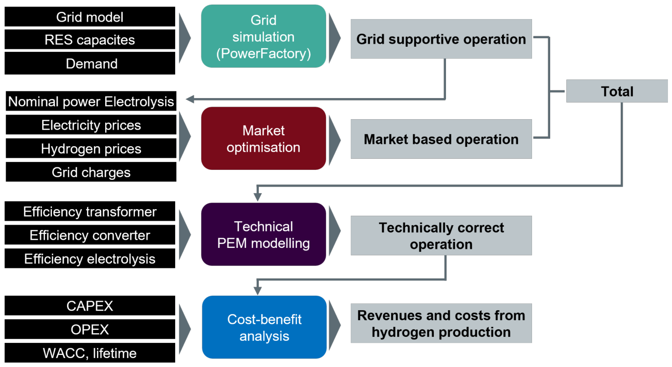
Figure 2.
Electricity-, gas and potential future hydrogen network in Styria in 2040, illustration by Energienetze Steiermark GmbH.
Figure 2.
Electricity-, gas and potential future hydrogen network in Styria in 2040, illustration by Energienetze Steiermark GmbH.
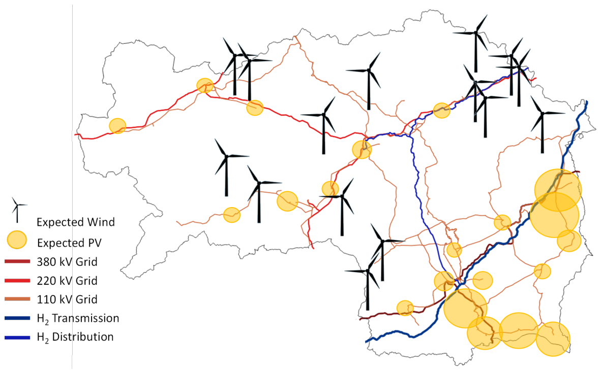
Figure 3.
Illustration of grid-supportive operation.
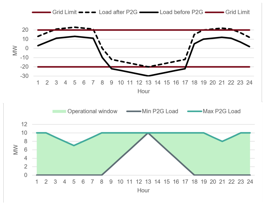
Figure 4.
Grid topologies.
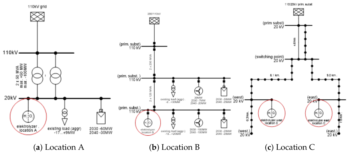
Figure 5.
Input assumptions on the development of renewable capacities.
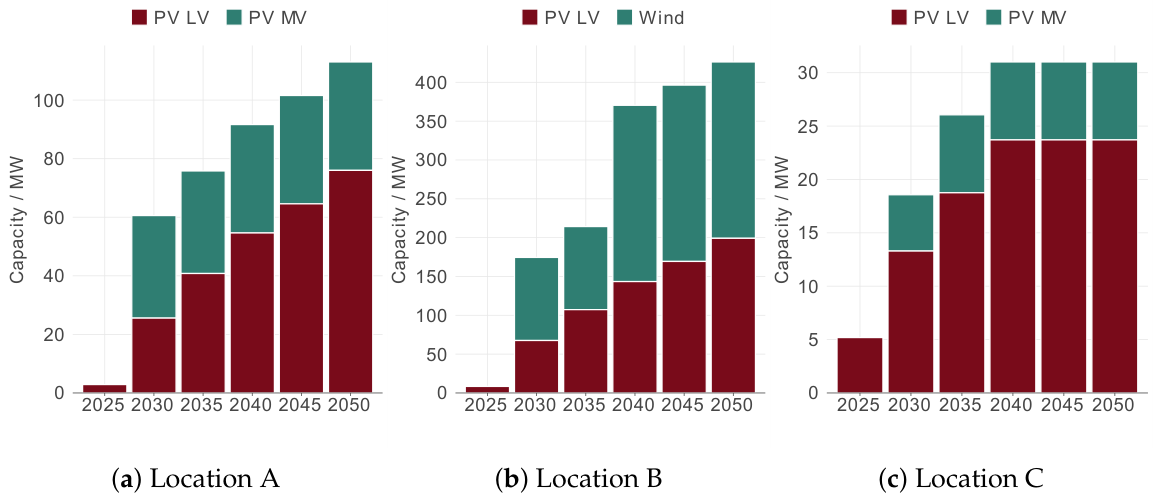
Figure 6.
Input assumptions on the development of demand.
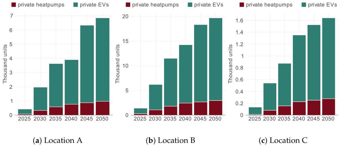
Figure 7.
Basic indicators of the baseline scenario: (a) lost energy and (b) lost revenues due to curtailment.
Figure 7.
Basic indicators of the baseline scenario: (a) lost energy and (b) lost revenues due to curtailment.
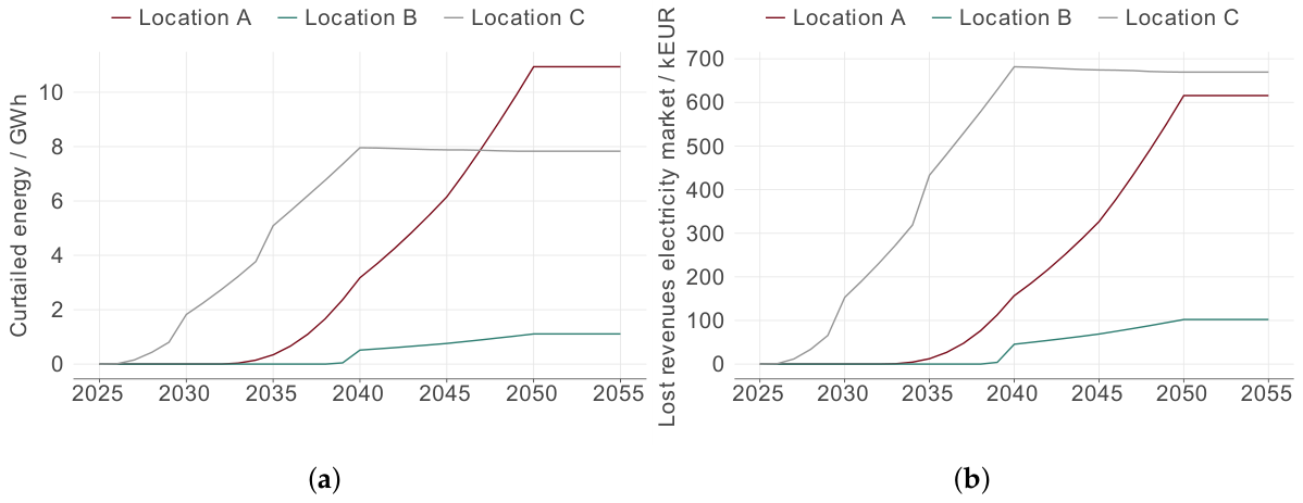
Figure 8.
Exemplary illustration of cost-benefit analysis for electrolysis in distribution grids.
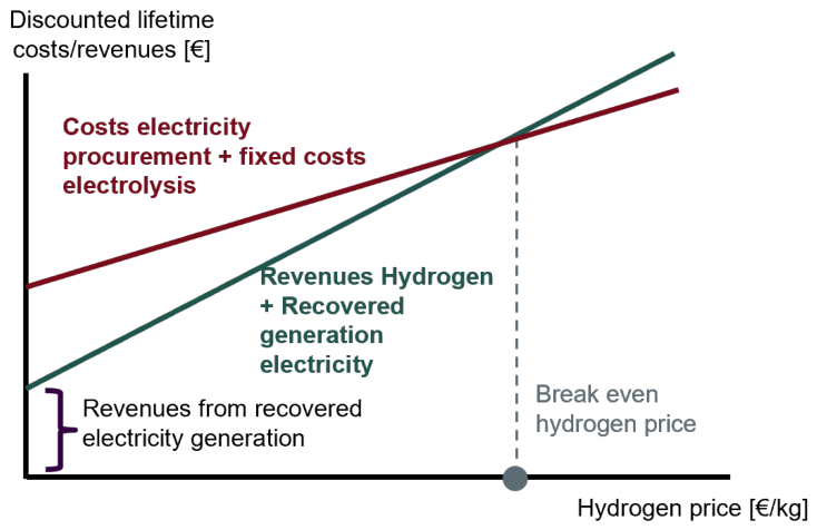
Figure 9.
(a) Nominal power of the electrolyzer and (b) corresponding full load hours.
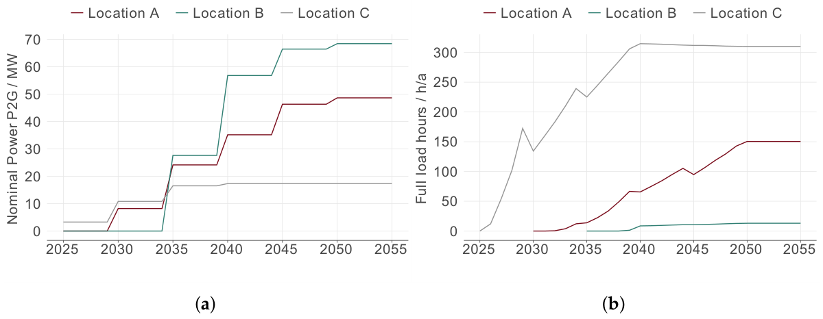
Figure 10.
(a) Electrolyzer full load hours in 2050 and (b) share of curtailment recovered through market based operation as a function of hydrogen prices.
Figure 10.
(a) Electrolyzer full load hours in 2050 and (b) share of curtailment recovered through market based operation as a function of hydrogen prices.
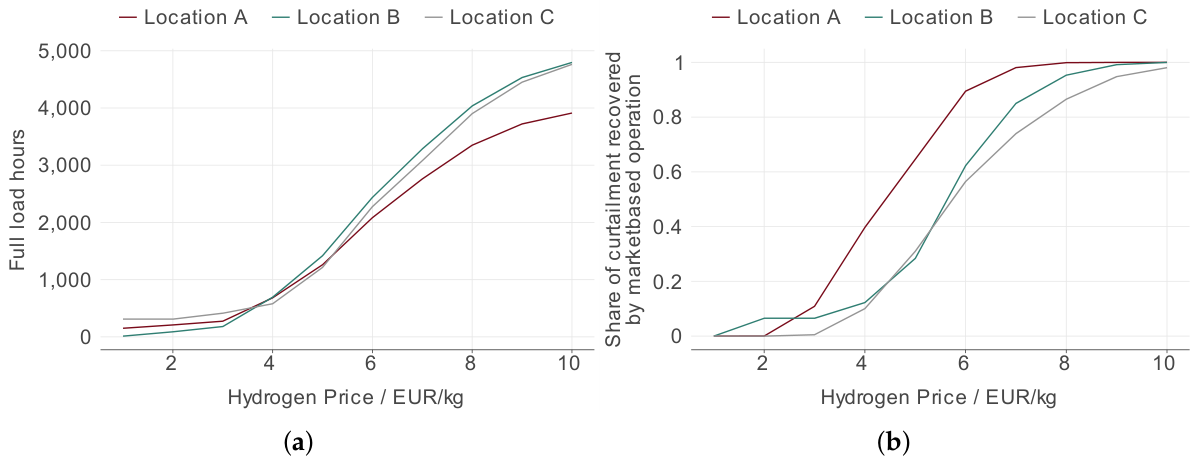
Figure 11.
(a) Share of curtailed revenues recovered and (b) break even hydrogen prices as a function of relative electrolyzer capacity.
Figure 11.
(a) Share of curtailed revenues recovered and (b) break even hydrogen prices as a function of relative electrolyzer capacity.
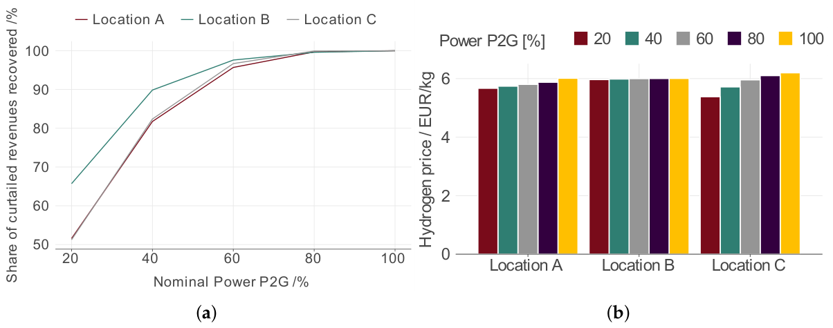
Figure 12.
Share of recovered electricity through market based operation under different electrolyzer nominal power.
Figure 12.
Share of recovered electricity through market based operation under different electrolyzer nominal power.
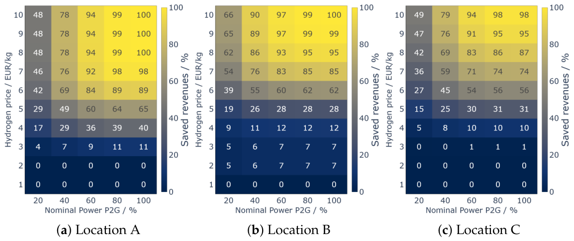
Figure 13.
CBA across different hydrogen price levels and electrolyzer capacities compared to conventional grid enforcement measures.
Figure 13.
CBA across different hydrogen price levels and electrolyzer capacities compared to conventional grid enforcement measures.
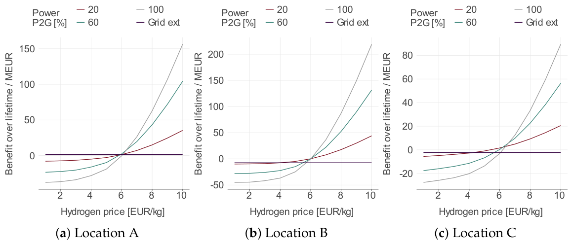

Table 1.
Grid charges for the year 2023 in the network area of Styria.
| Grid level | Peak load | Energy |
|---|---|---|
| 3 | 29,880 EUR/MW/a | 13.1 EUR/MWh |
| 4 | 35,520 EUR/MW/a | 18.4 EUR/MWh |
| 5 | 47,520 EUR/MW/a | 24.26 EUR/MWh |
Table 2.
Investment cost assumptions for electrolysis.
| 2025 | 2030 | 2040 | |
|---|---|---|---|
| CAPEX [EUR/kW] | 1,425 | 950 | 725 |
| OPEX [%/CAPEX/a] | 2 | 2 | 2 |
Table 3.
Estimated cost for conventional grid enforcement.
| P2G Location | Costs [MEUR] |
|---|---|
| Location A | 1.5 |
| Location B | 8 |
| Location C | 9.5 |
Disclaimer/Publisher’s Note: The statements, opinions and data contained in all publications are solely those of the individual author(s) and contributor(s) and not of MDPI and/or the editor(s). MDPI and/or the editor(s) disclaim responsibility for any injury to people or property resulting from any ideas, methods, instructions or products referred to in the content. |
© 2026 by the authors. Licensee MDPI, Basel, Switzerland. This article is an open access article distributed under the terms and conditions of the Creative Commons Attribution (CC BY) license (http://creativecommons.org/licenses/by/4.0/).
Copyright: This open access article is published under a Creative Commons CC BY 4.0 license, which permit the free download, distribution, and reuse, provided that the author and preprint are cited in any reuse.


