

Submitted:
16 July 2026
Posted:
17 July 2026
You are already at the latest version
Abstract
This paper presents a machine learning-based decision support system for multiclass defect detection, utilizing exclusively heterogeneous legacy process data to minimize manual inspection time in foundries. Validated on 51,377 products across 193 defect categories, the methodology resolves structural data inconsistencies through k-nearest neighbors (kNN) imputation and piecewise Winsorization. A multi-stage feature selection cascade, incorporating variance thresholding, correlation filtering, and Random Forest Feature Importance (RFFI), reduces the feature space from 139 to 78 process-critical variables. Following Synthetic Minority Over-sampling Technique (SMOTE)-based class balancing, five classifiers were benchmarked via 10-fold cross-validation and optimized using the macro-averaged F3-score to mathematically penalize undetected defects. Light Gradient Boosting Machine (LightGBM) and Random Forest (RF) provided superior predictive baselines. To enforce strict zero-defect constraints, an asymmetric risk function shifted decision boundaries, enabling risk-calibrated base models to reduce manual inspection volume by 9.2% with zero defect escapes. To resolve conflicting predictions, multi-algorithm decision fusion was implemented. By statistically evaluating the joint probabilities of the base models' post-calibration outputs, a Naive Bayes Stacking meta-classifier effectively neutralizes single-algorithm inductive biases. Ultimately, synthesizing these F3-optimized, risk-calibrated base models via meta-learning successfully isolated true defect-free components, maximizing the final inspection time reduction to 14.1% while strictly maintaining zero defect escapes.
Keywords:
multiclass defect classification
; decision fusion
; inspection time reduction
; ensemble learning
; SMOTE
; foundry defects
1. Introduction
Foundries represent a fundamental component of the European and global manufacturing sector. Most of these businesses are traditionally classified as small and medium-sized enterprises (SMEs), reflecting highly specialized product portfolios with complex geometries for dedicated customers in almost all major industries, such as construction, automotive, aerospace and heavy machinery [1]. Detecting and mitigating product defects is essential for economic and ecological sustainability. Quality defects drive high scrap rates, energy consumption, and material waste, directly conflicting with efficiency targets. To continuously reduce them, foundries rely on defect classification, i.e., detecting quality issues and categorizing them into distinct groups to enable targeted root-cause analysis and treatment.
These defects in foundries emerge from the complex interaction between material properties, equipment settings, and the execution of processes across multiple stages, such as melting, alloy treatment, moulding, casting, solidification, and finishing. In practice, metal-forming defects occur in different sizes, forms, and shapes and can be classified into distinct categories [2]. In this paper defects are mainly grouped into surface discontinuities/defects, volumetric porosities and inclusions (internal defects), as well as solidification and structural defects (Figure 1). Each category reflects distinct physical and metallurgical mechanisms. Given the variability and interdependence of sequential process steps, comprehensive real-time supervision of all defect-inducing factors often remains practically unachievable [3].
To mitigate these complex defects, a substantial proportion of extant literature on defect detection emphasizes post hoc identification and classification via vision sensors [5]. However, deploying vision-based inspection systems in foundries is itself challenging because the production environment is often harsh, with dust, heat, and other factors that complicate stable image acquisition. Moreover, these systems are inherently limited in identifying volumetric defects such as porosity and inclusions because such defects are not directly observable at the surface. Therefore, root-cause analysis of internal defects generally requires complementary techniques such as X-ray, computed tomography, or ultrasonic testing, often alongside complex 3D simulation data [7]. Thus, even with digital quality-assistance systems, critical quality decisions still largely depend on operators’ tacit domain knowledge. This expertise varies considerably across individuals, leading to inconsistent interpretations. As production becomes more dynamic, with shrinking lot sizes, increasing product complexity, and heterogeneous equipment, this variability in human expertise creates a growing need for decision support ( [8,9]).
Multiclass defect classification provides significant value because it enhances quality inspection by enabling targeted root-cause diagnosis and defect-specific mitigation, even for non-visible defects by linking predictions to likely root-cause factors. However, each classification objective faces distinct limitations, leading to a lack of transferability for even related processes ([10,11]). Consequently, merging operator-specific know-how with ML-based defect classification pipelines is becoming crucial to sustain reliable and efficient manufacturing performance. Yet, this is obstructed by data heterogeneity and poor quality in legacy databases [12]. Foundry production databases, accumulated through years of incremental automation, often contain structural inconsistencies that obscure defect-cause relationships. Because these historical records are frequently collected under varying and undocumented logging practices, they suffer from a range of data quality issues. These include machine-generated errors, such as duplicate entries and timestamp drift, as well as human-annotation errors like missing values and misclassified defect codes [13]. Furthermore, real-world production data is severely imbalanced: successful cycles vastly outnumber defect instances, causing standard algorithms to ignore critical minority defects. Therefore, robust model training necessitates a structured pre-processing pipeline that harmonizes heterogeneous data, reduces feature redundancy, and addresses class imbalance [14]. In such environments, standard evaluation metrics can become unreliable, as they fail to capture the asymmetric operational costs between false alarms (FAs) and undetected defects, necessitating specialized optimization functions ( [15,16]).
Hence, the objective of this paper is to develop a comprehensive decision support system that transforms heterogeneous foundry process data into multiclass defect predictions and actionable root-cause insights. By explicitly resolving structural data inconsistencies, missing values, outliers, and severe class imbalances through a robust machine learning pipeline, the proposed assistance system unlocks the latent value of existing production databases to directly support operator decision-making and quality assurance. The main contributions of this paper are summarized as follows:
- Development of a reproducible cleanup pipeline that employs format normalization, kNN-based imputation, and robust outlier filtering via winsorization to successfully transform fragmented, multi-stage process records into stable model inputs.
- Implementation of a systematic, multi-stage feature engineering pipeline by utilizing variance thresholding, correlation filtering, and RFFI. While this approach systematically prunes highly correlated and redundant parameters to reduce database dimensionality, it is deliberately designed to accommodate necessary operator intervention.
- Strategic application of the Synthetic Minority Over-sampling Technique (SMOTE) strictly within the training folds of a defect-stratified 10-fold CV. This ensures that critical but infrequent defect types are reliably learned and predicted, rather than being overshadowed by defect-free products.
- Systematic performance comparison of five classifiers (RF, XGBoost, LightGBM, AdaBoost, and kNN) on a real-world foundry dataset. To align with industrial quality standards, hyperparameter tuning and model evaluations were strictly governed by the macro-averaged F3-scores. This is an asymmetric metric intentionally selected to mathematically penalize critical missed defects over FAs.
- Application of a post-processing threshold calibration to enforce strict industrial zero-defect constraints. Utilizing confusion matrices (CM) to map continuous prediction probabilities against asymmetric misclassification costs, the decision support system systematically shifts default decision boundaries to safely act as a pre-filter for manual inspection.
- Implementation of post-calibration decision fusion strategies (e.g., hard voting, rule-based consensus) to synthesize predictions across multiple base models into a final operator assistance system. This stage evaluates whether combining independent classifiers, which have been individually risk-calibrated to be hyper-sensitive to defects, can systematically increase the manual inspection time reduction beyond the capacity of any single algorithm.
The remainder of this paper is organized as follows. After reviewing related work on industrial defect classification and data challenges in Section 2, the paper introduces the foundry dataset and the pre-processing and modeling pipeline in Section 3. Section 4 then presents the quantitative results and interpretability analyses, before Section 5 discusses deployment-related implications, operator integration, key findings, and future research directions.
2. Related Work
Given the data challenges outlined in Section 1, the related literature on ML-based defect classification in foundries generally exhibits two distinct methodological focuses: studies that prioritize the development of robust data preparation pipelines to resolve underlying database complexities, and studies that assume a static or pre-cleaned dataset to focus purely on the algorithmic performance of isolated classifiers.
Existing approaches in structuring data pipelines highlight that algorithmic success relies heavily on plant-specific pre-processing to analyze equipment data, such as mold types and binder materials [17]. Addressing inherent data constraints, specifically severe class imbalance, is a fundamental prerequisite in manufacturing contexts. Pipelines combining SMOTE with classifiers like XGBoost have been shown to significantly improve defect recognition [18], particularly when deriving feature importances to identify key factors of surface defects [19]. Similarly, the robust classification of cementite and porosity defects has been successfully demonstrated by utilizing SMOTE to balance data regarding casting temperatures and chemical analyses [20]. Furthermore, interpretability remains a critical component of these pipelines. Recent pipelines in sand casting provide operator feedback via feature importance visualization, offering interpretable insights into defect formation mechanisms such as permeability and moisture content [21].
To identify and classify specific defect classes, ensemble learning models applied to industrial datasets have demonstrated high classification accuracy. Applications include RF-based hybrid models in die casting, kNN models in gravity casting for multiclass defect classification [22], as well as RF and kNN models for classifying thickness deviations in refractory coatings [23]. Further applications indicate that classifiers based on decision trees and gradient boosting are particularly robust for isolating internal structural defects, such as micro-shrinkage and tensile anomalies [20]. In terms of feature engineering, surface defect studies have utilized XGBoost and RF to competitively isolate chemical and physical factors—such as binding agents and fines proportion—as principal drivers [24]. Further state-of-the-art research demonstrates that utilizing stacking ensembles and multi-model fusion on top of SMOTE-balanced data significantly outperforms isolated classifiers, successfully mitigating single-algorithm variance to achieve highly balanced precision and recall [25].
While these advancements provide a strong foundation for foundry defect classification, the primary emphasis in current literature remains on optimizing theoretical accuracy and post-hoc diagnostics. The translation of these models into deployed operator assistance systems, specifically utilizing decision fusion to safely bypass physical quality gates and actively reduce manual inspection time, remains underexplored. Furthermore, many existing approaches bypass the severe structural inconsistencies typical of raw production databases. Consequently, this paper addresses this gap by proposing a holistic methodology that systematically processes highly heterogeneous foundry data, calibrates base models for strict defect sensitivity, and utilizes multi-algorithm decision fusion to safely automate manual inspection time under zero-defect constraints.
3. Materials and Methods
This chapter details the proposed architecture of the decision support system for multiclass defect classification utilizing heterogeneous foundry process data. The methodology, illustrated in Figure 2, is designed as a sequential pipeline. It initiates with data acquisition and format normalization (Section 3.1), followed by a structured data cleanup and feature engineering phase to resolve structural database inconsistencies (Section 3.2). Subsequently, the pipeline handles severe class imbalance prior to model training and hyperparameter tuning (Section 3.3). The methodology concludes with a risk-calibrated evaluation phase, utilizing confusion matrices and multi-algorithm decision fusion to securely optimize inspection routing (Section 3.4).
3.1. Foundry Database Acquisition & Pre-Processing
The dataset integrates two primary sources: a production database (df_main) containing process and product parameters. In total, it captures 139 features across 51,377 unique products, spanning general parameters (49 columns), geometric dimensions (27), temperatures (15), velocities (6), material properties (10), and process durations (18). However, the raw data exhibits significant heterogeneity, including mixed measurement units, non-standard text formatting, and visible gaps in sensor readings. Figure 3 and Figure 4 visualize the critical integrity issues addressed in this pipeline:
- Completeness & Distribution: Red cells indicate missing values, while blue cells highlight distributional skew and implausible spikes.
- Consistency: Pink cells denote mixed units within single columns and also potential writing errors.
- Relational Integrity: Orange cells reveal duplicate rows, grey cells mark faulty/non-monotonic timestamps, and light-brown cells indicate misaligned joins in the main database between different product samples.
Quality outcomes are stored in a separate product defect database (df_defect) (Figure 5), where trained operators assign specifically derived defect identificators (DefectID) based on plant quality guidelines. Together with respective labels (DefectLabel), they are organized into a taxonomy covering major defect families such as porosity, shrinkage, surface discontinuities, and dimensional errors. Each record is linked to the main production table via a unique product number (ProdNr) and includes a Severity Index (SEVERITY) ranging from 0 (least severe) to 10 (most severe). For products exhibiting multiple defects, only the highest-severity defect is retained to ensure a strictly one-to-one mapping between input features and target labels. After reconciling this table and filtering for valid multi-defect cases, it contains 22,915 defect events mapped to 13,338 uniquely defective products across 193 distinct defect types selected by operators.
To establish a ML-compatible foundation, essential format normalization and schema validation steps were first applied to the entire merged dataset. This initial preparation harmonizes basic measurement units and categorical encodings across the production and defect tables. Text fields containing embedded units or inconsistent delimiters were parsed into numerical values, with parsing failures safely coerced to missing values (NaN) to prevent pipeline disruption. Categorical attributes were normalized to consistent spelling schemes via label encoding. Furthermore, schema validation enforced data type coercion, resolved parsing errors, deduplicated entries, and validated primary/foreign key relational integrity. For products exhibiting multiple defect entries, records were aggregated by maximum severity index to ensure a strict one-to-one feature-label mapping, while undocumented products were classified as the defect-free baseline. Beyond preparing the data for immediate algorithmic modeling, identifying these structural inconsistencies enabled the derivation of long-term optimization strategies for the foundry’s ongoing database management and data collection practices. Subsequently, an 80/20 stratified random split was employed to divide the data into a training set and a held-out test set. This stratification was executed strictly with respect to the target defect class vector, ensuring that the heavily imbalanced proportional representation of specific defect types was preserved perfectly, independent of the input feature distribution.
3.2. Data Cleanup & Feature Engineering
Legacy foundry databases accumulate structural inconsistencies from incremental automation—mixed measurement units, non-standard text formatting, missing values, duplicate entries, and relational misalignments. This section presents a systematic pipeline converting heterogeneous records into stable numeric/categorical inputs suitable for downstream modeling. These learned parameters are used to process the training dataset and are subsequently applied to the held-out test set.
3.2.1. kNN-Based Imputation
To resolve missing values inherent in foundry records, the pipeline employs kNN imputation. In this context, kNN estimates a missing value by identifying historical production cycles (neighbors) that exhibit the shortest mathematical distance, which is the highest overall similarity in their recorded process parameters, to the incomplete record. However, calculating this multidimensional distance is highly sensitive to noise and data sparsity when applied indiscriminately. If highly volatile or statistically isolated sensor variables are included, the distance calculation can become distorted. To address this, the proposed methodology introduces a strict statistical eligibility screening. Features qualify for imputation only if they satisfy three conditions: a maximum acceptable missingness rate θkNN,miss, coefficient of variation bound θkNN,CV, and minimum correlation support with other process variables. Mathematically, a feature j must satisfy the following:
where the first condition limits the proportion of missing values to the threshold θkNN,miss, the second condition bounds the coefficient of variation using the feature’s standard deviation and mean below θkNN,CV, and the third condition ensures minimum correlation support by requiring an absolute pearson correlation of at least with at least one other feature m. For eligible features, the algorithm utilizes the NaN-aware Euclidean distance (i.e., L2-Norm) between two sample vectors x and y, which ignores missing dimensions during neighbor selection [26]:
with N is the total number of features, counts observed dimensions where both values are present and the indicator function equal to 1 if neither nor is NaN, and 0 otherwise. Once the distances are calculated, the nearest neighbors (sorted by distance) are identified. The missing value for feature j in sample x is then estimated via mean imputation, preserving the local geometric structure of the process data:
Features failing the initial screening, due to excessive missingness, volatility, or statistical isolation, are excluded from the pipeline to prevent the propagation of bias. A balanced mitigates the influence of random sensor noise without averaging across fundamentally different operating states, which would otherwise destroy local process patterns.
3.2.2. Variance Treshold Filtering (VTF)
High-dimensional foundry data captures hundreds of sensor readings, but fixed machine settings and inactive channels exhibit negligible variance representing measurement noise rather than physical signals. VTF requires complete numeric input post-imputation, evaluating intrinsic feature variability independently of target labels. For continuous feature j with n samples, the empirical sample variance quantifies signal strength [27]. A feature is retained only if its variance meets or exceeds a predefined threshold :
with as the value of feature j for sample i, and as the mean. Features failing this condition are pruned from the dataset as non-informative noise.
3.2.3. Winsorization
Continuous manufacturing sensors often produce extreme outliers due to electrical interference or calibration errors. Traditional interquartile range (IQR)-based trimming discards entire records containing outliers, which severely depletes already scarce minority-class defect samples. To address this, Winsorization implements piecewise percentile capping, mitigating extreme values while preserving the overall sample size. For a continuous feature x with lower and upper percentiles qlow and qup calculated at lower and upper quantiles αlow and αup , the winsorized value W() for an observation is defined as [28]:
By capping extreme values at these data-driven percentiles (= = 0), winsorization constrains sensor anomalies to empirically plausible ranges.
3.2.4. Pearson Correlation Filtering (PCF)
Manufacturing datasets frequently capture identical physical phenomena through multiple redundant sensors, such as adjacent thermocouples or duplicate machine setpoints. This resulting high multicollinearity inflates model variance and distorts downstream feature importance scores. To address this, the pipeline calculates the pearson correlation matrix RP ∈ to identify highly correlated feature pairs. For two continuous features x and y with n samples, the correlation coefficient is computed as [29]:
If the absolute correlation between any two features exceeds a predefined redundancy threshold (∣∣ > ), they are flagged as capturing overlapping information. To resolve this multicollinearity without losing critical information, only one feature from the redundant pair is pruned. The decision of which feature to remove is driven by practical heuristics: the pipeline retains the feature that exhibits higher sample variance, possesses higher initial feature importance derived from RF, or offers greater interpretability for human operators.
3.2.5. RFFI-Based Feature Deselection
The final step of dimensionality reduction employs a baseline RF as an embedded feature selector to capture nonlinear interactions between process parameters and defect formation. For a multiclass problem with c distinct defect classes, the algorithm evaluates how effectively a feature separates these classes. In decision tree logic, a node contains a subset of the production data. The impurity of this node refers to how mixed the defect classes are within that subset. A highly impure node contains many different defect types, while a pure node contains predominantly one type. This impurity is measured mathematically using the Gini index [30]:
where represents the empirical fraction of samples belonging to defect class c at node . When node is split into two smaller subsets using a continuous feature j, the goal is to create subsets that are purer than the parent. The resulting “split gain”—defined as the decrease in impurity achieved by this split—is calculated as:
With as the total number of samples present at the parent node . and denote the number of samples routed to the left child node () and right child node (), respectively. This weighting ensures that splits successfully separating large portions of the dataset are rewarded more heavily than splits isolating only a few outliers. To determine the global feature importance for feature j, the algorithm aggregates these weighted split gains across the entire forest. This is calculated by summing the impurity decreases over all nodes where j was used to split, and averaging across all trees:
In which is the total number of decision trees in the forest, and represents an individual tree. The inner summation iterates exclusively over the subset of nodes within where j was chosen as the splitting variable. The term scales the gain by the proportion of total training samples that passed through . Features with a global importance score falling below a predefined threshold are pruned. However, in alignment with industrial requirements, this pruning is finally still subject to operator validation. Thus, variables heuristically deemed essential for post-hoc root-cause diagnostics are actively retained.
3.3. Model Development & Tuning
Because foundry defect datasets exhibit pronounced class imbalance, with certain defect types being severely underrepresented, SMOTE is applied to the training set. Furthermore, this section outlines the theoretical foundations and implementation strategies for the five classification algorithms evaluated in this study: RF, kNN, XGBoost, LightGBM, and AdaBoost. To optimize predictive performance, hyperparameter tuning is conducted using a randomized search coupled with 10-fold stratified cross-validation. For each model, a predefined hyperparameter space is explored by sampling from distributions appropriate to each parameter type.
3.3.1. Handling Class Imbalance with SMOTE
To address severe class imbalance, SMOTE is applied exclusively to the training data. Let Cmaj denote the majority class (defect-free) with Nmaj samples, and let Cmin,c denote a specific minority defect class with Nc samples, where . The objective of the multiclass SMOTE application is to determine a class-specific oversampling ratio Sc such that the synthesized dataset achieves parity:
For each required synthetic sample in Cmin,c, SMOTE avoids exact duplication, which induces overfitting, by algorithmically interpolating within the local geometric feature space. Thus, for a minority-class observation in a p-dimensional feature space, its k nearest minority neighbors, i.e., from the same c, are identified. A synthetic observation is generated by convex interpolation:
where is a randomly chosen neighbor. The sampling strategy raises all minority classes to the size of the majority class.
3.3.2. Ensemble Classifiers
Five classifiers are evaluated, representing different learning paradigms:
- RF [32]: An ensemble of bagged decision trees trained with the Gini impurity criterion. It handles mixed data types without scaling and provides feature importance estimates. The number of trees (n_estimators), tree depth (max_depth), minimum samples per leaf (min_samples_leaf), and the number of features considered at each split (max_features) are tuned.
- kNN [33]: A non-parametric, instance-based classifier that assigns a class by majority vote among the kNN closest training samples. Distances are computed with the Manhattan metric (L1-norm) after standardizing the features to ensure equal contribution. The voting scheme dictates how neighbors influence the prediction, i.e., either via uniform weighting, where all kNN neighbors contribute equally to the majority vote, or distance-based weighting, where closer neighbors exert a stronger influence on the final class assignment than more distant ones.
- XGBoost [34]: A regularized gradient boosting method that builds an additive model of shallow decision trees. It uses a second-order Taylor expansion of the loss function and includes L1/L2 regularization on leaf weights. Key tuned parameters are the learning rate (η), tree depth (max_depth), number of trees (n_estimators), subsampling ratios, and regularization strengths ().
- LightGBM [35]: A gradient boosting implementation that grows trees leaf-wise, focusing on the leaf with the highest loss reduction. It uses histogram-based algorithms for efficiency. Tuned hyperparameters include the number of leaves (num_leaves), tree depth (max_depth), learning rate (η), number of trees, minimum child samples, and L1/L2 regularization.
- AdaBoost [36]: AdaBoost was implemented in its Stagewise Additive Modeling using a Multi-class Exponential loss function (SAMME) variant to support the multiclass defect classification setting. The model sequentially fits weak learners, increasing the weight of previously misclassified samples so that later learners focus on harder observations. In this study, the number of estimators (n_estimators) and the learning rate (η) were tuned on the training folds, while the base learner consisted of decision stumps.
The hyperparameter search spaces listed in Table 1 were defined based on prior empirical knowledge from the literature and preliminary experiments. To efficiently explore these spaces, a randomized search was employed, sampling different configurations from the respective search spaces for each model architecture. The final hyperparameter values listed in the rightmost column correspond to the configuration that achieved the highest cross-validated macro- score.
3.3.3. k-Fold CV
Hyperparameter optimization was performed via randomized search with stratified 10-fold CV using macro- score as the selection criterion. For each model architecture, a predefined number of hyperparameter configurations niter was randomly sampled from the search space defined in Table 1, where each configuration represents one complete combination of candidate hyperparameter values. To avoid notation overlap with subsequent classification thresholds, let ξ denote a specific hyperparameter configuration. The cross-validated performance estimate for ξ is calculated as [37]:
where is the model trained on the i-th training fold using ξ and evaluated on the corresponding validation fold . The configuration achieving the highest mean CV score was selected as optimal. This optimal cross-validated mean is subsequently compared against the independent test set performance to evaluate out-of-sample stability. Specifically, a significant degradation from the CV mean indicates potential overfitting to the SMOTE-augmented training distributions, whereas aligned scores validate robust generalization.
3.4. Classification Performance Evaluation
Standard classification accuracy is misleading under severe class imbalance because a model can achieve high accuracy by simply predicting the majority class. Consequently, macro-averaged metrics and threshold-sensitive diagnostics were adopted to ensure a robust performance evaluation across all rare defect types.
3.4.1. Macro-Averaged -Score
For a given class, precision and recall are defined from the CM elements (true positives TP, false positives FP, false negatives FN) [38]:
Industrial quality control features a severe risk asymmetry: undetected defects (false negative, FN) incur vastly higher costs than manual re-inspections caused by FAs (FP). To mathematically embed this asymmetric risk into the model evaluation, the generalized Fβ-score is utilized [39]:
By setting β it weights recall more heavily than precision, strictly penalizing missed defects. Finally, to evaluate the multiclass objective, the unweighted arithmetic mean across all classes the macro-averaged -score is computed. This ensures that rare defect types influence the final metric equally to the defect-free majority class, neutralizing the dataset’s inherent imbalance.
3.4.2. CM and Sensitivity-Driven Thresholding
CM is a fundamental diagnostic tool in multiclass classification that tabulates predictions against true labels. For a kCM-class problem, the CM has entries
where N is the total number of samples, is the true label, the predicted label for sample n and I(.) is the indicator function. CM analysis complements the scalar definitions in the -score section by exposing per-class error structures and pairwise confusions. For interpretability, row-normalized matrices
express the distribution of predicted classes for each true class i. Heatmaps of visually highlight systematic mix-ups between specific classes (confusion blocks) and reveal minority-class failure modes that aggregated scalar metrics may obscure.
Although the decision support system predicts specific multiclass defects, the final automated routing decision is strictly binary: a component is either safely released (True Negative, TN) or flagged for manual review. To facilitate this, the multiclass confusion matrix is collapsed by grouping all specific defect types into a single ‘Positive’ (Defective) class, leaving the defect-free state as the ‘Negative’ class. Consequently, False Positives (FPs) represent safe but redundant manual inspections, whereas False Negatives (FNs) constitute critical defect escapes. Because conservative foundry production penalizes FNs far more heavily than FPs, the standard maximum probability rule is insufficient. Instead, a component is assigned to the defect-free class (OK) only if its predicted posterior probability strictly satisfies a predefined, risk-calibrated safety threshold . Otherwise, the system defaults to flagging the component for manual review by predicting the most probable defect class , formulated as:
By optimizing by an asymmetric risk function R():
where is the cost of a FA and is the penalty for defect escape, with and denoting the total number of false positives and false negatives, respectively, yielded by the classifier at a given threshold CM. By applying a heavily skewed penalty weight, the optimization strictly constrains to zero. While this inherently increases FP rates, it guarantees that all components confidently predicted as defect-free (TN) can safely bypass manual inspection. Flagged components are routed to conventional manual review, ensuring the overall defect escape rate never exceeds the current manual baseline.
3.4.3. Decision Fusion
While single classifiers can be individually calibrated to minimize empirical risk, they remain susceptible to varying inductive biases, particularly in highly imbalanced tabular manufacturing data [41]. To stabilize the final prediction boundary and maximize inspection time reduction while strictly maintaining the zero-defect escape mandate, a post-calibration decision fusion pipeline was implemented.
Let represent the ensemble of trained base classifiers. For a given component feature vector , each model outputs a posterior probability for the defect-free class, . To account for asymmetric industrial costs, where the penalty for a defect escape exponentially outweighs a FA, this continuous probability is mapped to a discrete class label using an individually optimized decision threshold . The base prediction is defined via the indicator function :
where denotes a safe ‘OK’ routing, and denotes a ‘NOK’ routing to manual inspection. Rather than exhaustively computing heuristic combinations, four specific, mathematically distinct fusion paradigms were evaluated to synthesize these outputs:
- Majority Voting:
Established as the standard baseline for decision fusion, majority voting evaluates the deterministic, risk-calibrated outputs of the individual models. The ensemble flags a component for inspection if the strict mathematical majority of the base models predict a defect:
In addition to “hard majority voting”, we also evaluated a relaxed consensus rule “At Least 2 Oks” for the five base classifiers. In this rule, the final sample-level decision is routed to the defect-free class when at least two of five models vote OK; equivalently, the sample is routed to manual inspection when at least three models vote NOK. This variant was included to test whether a less conservative aggregation rule can further increase inspection-time reduction while preserving the zero-escape constraint.
- 2.
- Penalized Weighted Voting:
Standard majority voting implicitly assumes equal competence of all base classifiers. To reduce FPs without increasing defect escapes (FNs), we introduce a penalized weighted voting scheme in which each model m receives a validation reliability weight derived from its cross-validated multiclass defect classification performance. The final vote aggregation combines overall validation reliability with defect-class-specific performance, thereby assigning greater influence to classifiers that perform well for the respective fault category while down-weighting inconsistent or weak defect predictions. Let denote the predicted class of model mm for sample i, and let c denote a candidate class. The class-wise ensemble score is computed as
Classifiers with higher cross-validated reliability contribute more strongly to the ensemble decision, while less reliable predictions for a given defect class are down-weighted through a penalty factor , resulting in
The final multiclass ensemble prediction is then obtained as
- 3.
- Naïve Bayes Stacking:
To replace human-designed consensus heuristics with a statistically optimal synthesis, Naïve Bayes Stacking was applied as a meta-classifier. The continuous probability outputs from the base ensemble form a new feature vector . A Gaussian Naive Bayes meta-classifier is then trained on the validation folds to map to the final routing label. By maximizing the posterior probability based directly on the combined algorithmic distributions, this approach learns to intrinsically resolve conflicting evidence across the base models.
3.5. Implementation Details
All experiments were implemented in Python 3.12.4. ML models were built using scikit-learn (v1.5.1) for RF, kNN, AdaBoost, Stacking, and probability calibration, alongside XGBoost (v2.0.3) and LightGBM (v4.3.0). Data resampling was performed with imbalanced-learn (v0.12.3) using SMOTE. Hyperparameter optimization was executed using RandomizedSearchCV from scikit-learn, with parallelization managed directly within the compatible base estimators to optimize computational efficiency.
4. Results & Discussion
4.1. Data Pre-Processing Pipeline Performance
4.1.1. Initial Dataset Characterization
The merged production and defect datasets comprised 51,377 production units and 22,915 defect events spanning 193 distinct defect types. Prior to modeling, defect classes with a relative frequency below 2% in the training distribution were removed to ensure statistical reliability and to avoid overfitting to extremely rare patterns. This pruning reduced the number of active defect categories to 53 dominant defect classes plus the defect-free baseline, retaining a total of 44,665 valid product samples. This step preserved the most critical failure modes while maintaining high interpretability and diagnostic focus for shop-floor operators.
4.1.2. Missing Data Resolution
The effectiveness of imputation was assessed by comparing the proportion of valid entries before and after the procedure. Before any imputation, df_main contains 5.571.945 valid entries out of 7.141.403 total (= 78.02%), as is qualitatively depicted in Figure 6. A valid entry was defined as a numeric value (interpretable as a float or integer) that was not missing (NaN) and not corrupted by non-numeric content. The total number of valid entries was computed for the dataset as:
with the number of rows, the number of columns, as a test function for valid entries and as a test function for non-valid entries. The overall validity ratio is subsequently calculated as .
To complement the quantitative analysis of data validity, a qualitative visualization was introduced by plotting the structure of valid and non-valid entries across the dataset. In this plot, valid data points are visually distinguished from non-valid entries (such as missing or corrupted values), typically using a missingness map with binary color scheme (e.g., black for valid, white for non-valid) [42]. This approach enables an immediate visual assessment of data integrity patterns across different variables and observations. The cleanup process is complemented by the unification of formatting via label encoding similar to [43], which ensures interpretability and preserves ordinal independence, especially over one-hot encoding, which, while common, may introduce artificial relationships in categorical inputs. The raw process/features table exhibits heterogeneous numeric and textual fields, unit strings embedded in values, and non-random missingness patterns. First, format normalization coerces leading numeric tokens to floats (non-imputable values become NaN) and applies label encoding to selected categorical fields to preserve ordinal independence.
Following the multi-stage filtering described in Section 3.2.1, only numeric variables meeting strict eligibility criteria (missingness kNN,miss ≤ 40%, coefficient of variation kNN,CV ≤ 0.8, and kNN,corr |r| ≥ 0.6 with at least one other column) were retained for kNN imputation. For those columns, a KNN imputer with kkNN = 50 and nan-aware Euclidean distance metric was applied. This targeted geometric reconstruction raised the overall dataset validity ratio to = 84.51%. Variables that did not satisfy the eligibility criteria were excluded from geometric reconstruction and handled by simpler completion rules (e.g., constant placeholder) where necessary.
4.1.3. Outlier Control via Winsorization and VTF
Prior to imputation, the 0.5th/99.5th percentile Winsorization capped extreme values without discarding entire records, thereby preserving scarce minority-class samples. To visualize the effect of Winsorization, boxplots of the four features with the most extreme outliers (based on the ratio of maximum deviation from the median to IQR) were generated (see Figure 7). All outliers were examined individually, and features with narrow valid ranges (e.g., temperature peaks, cycle times, or material properties) were cleaned based on engineering judgement and visual analysis. In several cases, single-value peaks were clearly linked to sensor failures or misrecorded batches. Following imputation, a VTF (= 0.02) eliminated near-constant features, reducing the feature count from 139 to 104. In this highly heterogeneous industrial dataset, parameters that exhibit minimal variability across a large number of production units are often indicative of measurement redundancies, non-informative control parameters, or static setpoints that do not contribute significantly to classification tasks. This step also removed columns with no operational significance (e.g., unnamed indexing columns) after consultation with domain experts. By removing these uninformative columns, the validity ratio increased further to = 90.44%, thereby providing a solid foundation for the subsequent classification.
4.1.4. Feature Selection Results
After pre-processing, the feature space remained high-dimensional, containing subsets that were either heavily redundant or weakly informative for technical interpretation. Consequently, the feature set was refined using a complementary, two-stage sequential selection procedure. First, to resolve multicollinearity, pairwise pearson correlations were computed. Feature pairs exhibiting an absolute correlation of ∣r∣ > 0.995 were flagged as redundant. To resolve these overlaps, one feature from each highly correlated pair was removed based on lower variance or reduced technical interpretability. A qualitative assessment of the correlation heatmaps before and after this filtering (Figure 8) visually confirms the effective elimination of dense collinear blocks. This initial step removed 22 redundant features, reducing the feature count to 82.
With multicollinearity eliminated, a baseline RF classifier (B = 50, max_depth = 12) was subsequently trained on the correlation-reduced data to extract impurity-based feature importances. Features falling into the lowest 5th percentile of importance scores were flagged for removal. Rather than relying on a blind statistical cut-off, these low-importance features were reviewed for domain plausibility with operators before final action, ensuring that no domain-critical variables were inadvertently discarded. While these parameters generally correspond to physically plausible process parameters (e.g., cycle durations), their extremely low variance or low predictive power in this specific dataset justifies their removal without compromising the model’s diagnostic capacity. The normalized importance scores for the 20 most and 20 least important features are shown in Figure 9. Ultimately, RFFI removed additional 4 features, yielding a refined, highly interpretable final feature set of 78 variables.
4.2. Defect Classification Performance
The evaluation of classification performance is strictly framed around the primary industrial objective: acting as a highly confident pre-filter to safely minimize the manual inspection time of foundry components. Under the current status quo, manual inspection is performed on all products. Consequently, every product flagged by the ML model as defective, whether correctly (TP) or incorrectly (FP), will simply be routed to manual analysis, which would have occurred anyway. The true value of the system lies entirely in its ability to predict defect-free parts with such high confidence that they can safely bypass this manual review. Because an undetected defect (FN) reaching a customer incurs severe financial and reputational penalties, the models must operate with near-zero defect escapes. Traditional metrics like global accuracy are therefore inadequate. Instead, a successful model must achieve two simultaneous goals: it must maximize defect detection (recall) to prevent any escapes, and it must confidently identify true defect-free parts (TN) to significantly reduce the current 100% manual inspection time for the remaining.
To optimize for this asymmetric risk profile, a comparative evaluation of five classifiers (RF, LightGBM, XGBoost, kNN, AdaBoost) was conducted on the fully pre-processed dataset. Hyperparameter optimization was performed via a randomized search with 10-fold cross-validation strictly stratified along the target defect vector, explicitly utilizing the macro- score as the primary selection criterion mathematically penalizing the models significantly more for missed defects than for FAs during the training phase.
4.2.1. Macro-Averaged Classification Metrics
Table 2 reports the macro-averaged precision, recall, and -score for each classifier on the held-out test set (20% of the data; ). Because the overarching goal is to deploy an decision support system that conservative foundries can trust, the evaluation heavily weights recall via the score to explicitly penalize missed defects. Under this rigorous evaluation, LightGBM achieves the highest (0.397), demonstrating superior defect capture capability, followed by kNN (0.364) and RF (0.361). XGBoost achieved an of 0.344, while AdaBoost demonstrated the weakest overall performance at 0.309.
The modest -scores reflect the inherent challenge of distinguishing multiple subtle defect classes from noisy, highly imbalanced legacy manufacturing data, without installing new sensor infrastructure. As intended by the -driven optimization, the algorithms strictly prioritize recall to minimize critical defect escapes. This uncompromising focus on defect sensitivity ensures the operational reliability required to secure operator buy-in in risk-averse plants. By maximizing defect capture while maintaining the highest relative precision, LightGBM provides the most robust predictive baseline. This establishes the highly accurate foundation necessary for the subsequent risk-sensitive threshold calibration, which ultimately translates these baseline predictions into a safe, automated reduction in manual inspection time.
4.2.2. Cross-Validation vs. Test Set Robustness
To assess fitting behavior and out-of-sample robustness, models were tuned with stratified 10-fold cross-validation and then evaluated on an independent held-out test set. Figure 10 shows the cross-validated macro -score (blue bar shows mean across folds; whiskers with ±1 standard deviation) together with the test macro -score (red marker) for each model, based on results from Table 2. Bars with short whiskers indicate low fold-to-fold variance (stable fits), while a large vertical gap between the bar and the red marker indicates optimism in CV or distribution shift to the hold-out. LightGBM and RF show highest stability, with test scores slightly exceeding their cross-validated means, indicating robust generalization. XGBoost and kNN performed almost exactly in line with their cross-validation expectations. Conversely, AdaBoost fell below its cross-validation mean, highlighting a slight over-fitting to the synthetic balanced data generated by SMOTE. This behavior underscores the importance of evaluating models on a separate, unmodified test set to obtain realistic performance estimates.
4.2.3. CM and Risk-Sensitive Evaluation
The exact error structures of the models, before and after threshold calibration, are visualized using CM. For an enhanced visual comparability, the reported confusion matrices are shown in binary form, where all defect categories are collapsed into one NOK class and compared against the OK class. This binarization is used only for visualization and inspection-routing analysis; the underlying classifiers remain multiclass models trained and evaluated on the full defect taxonomy. To illustrate the shift in decision boundaries, Figure 11 contrasts the binary OK/NOK routing at the default maximum-probability rule (τCM,default = 0.5) with the optimized risk threshold. Specifically, XGBoost failed to detect 67.0% of all defective components (FN), followed by RF (64.1%), AdaBoost (59.4%), LightGBM (56.4%), and kNN (55.7%). Without calibration, these standard decision boundaries introduce critical reliability deficits.
Figure 12.
Binary CM at risk-calibrated threshold τCM,risk.
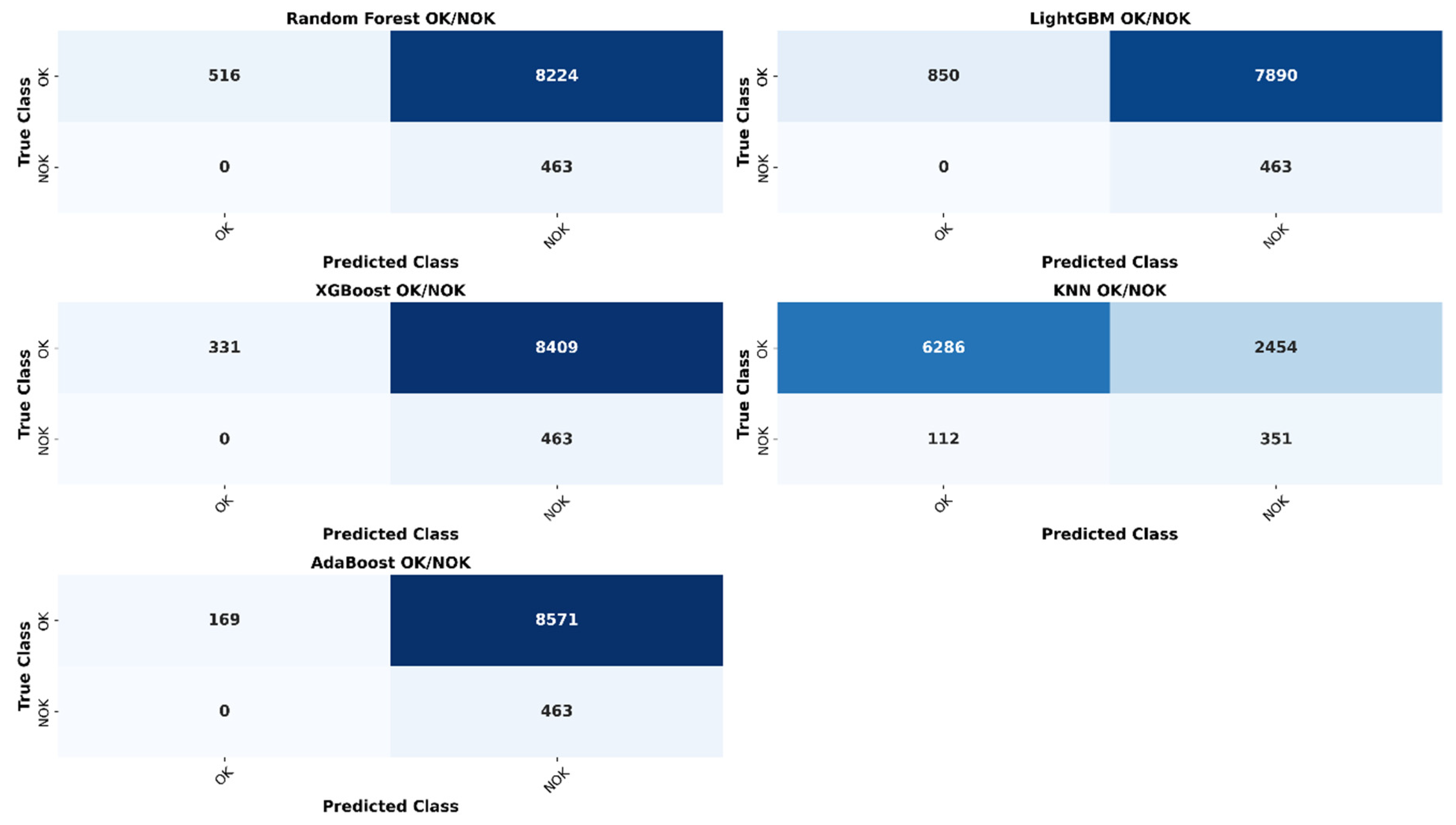
Applying the risk-sensitive calibration function R(τCM,risk) enforced a strict confidence threshold for the OK class, systematically overriding uncertain predictions and shifting them toward the manual inspection route. By minimizing this asymmetric risk function, the optimization successfully neutralized defect escapes (achieving 0% FN) for LightGBM, RF, XGBoost, and AdaBoost, successfully capturing 100% of the defective components in the test set. Conversely, kNN failed to satisfy this critical safety constraint, leaving 24.2% of defective components undetected even at the maximum permissible threshold (τCM,risk = 0.999), thereby disqualifying it for industrial deployment. Among the viable zero-escape models, the capacity to retain TN varied significantly due to differences in their underlying probability distributions. Under the strict thresholding logic which forces the models to only classify a part as ‘defect-free’ if their mathematical certainty is exceptionally high, LightGBM (τCM,risk = 0.999) maintained sufficient confidence to safely bypass manual inspection for a subset of defect-free components, achieving an overall inspection time reduction of 9.72%. RF (τCM,risk = 0.998) and XGBoost (τCM,risk = 0.983) proved overly conservative, yielding inspection time reductions of only 5.9% and 3.79%, respectively. AdaBoost (τCM,risk = 0.922) performed worst, yielding a marginal 1.9% inspection time reduction.
As shown in Figure 13, combining these calibrated models through decision fusion further improved the inspection time reduction. However, comparing the different fusion methods highlights a clear difference between using simple voting rules and using statistical meta-learning—where a higher-level algorithm mathematically learns how to optimally combine the predictions of the base models.
Standard Hard Voting maintained the zero-escape mandate but proved overly cautious, routing 8,300 components to manual review (5.03% inspection time reduction). Because the base models were already individually calibrated to be hypersensitive to defects, a standard voting rule amplifies this sensitivity. Under hard voting, if even a single highly penalized classifier flags a potential anomaly, the entire ensemble defaults to a manual review, leading to a compounding effect of FAs and massive redundant inspections. Implementing an agreement-penalized weighting scheme successfully mitigated this caution by moving away from equal veto power. Rather than treating all “NOK” predictions equally, this method applies a calculated penalty to base models that exhibited high FP rates during CV. Consequently, if an overly sensitive base model consistently contradicts the more precise models, its veto power is mathematically diminished. By overriding these unreliable warnings, this scheme safely rescued true defect-free parts from unnecessary manual inspection, significantly improving the inspection time reduction to 14.1%.
Finally, the implementation of Meta-Classifier Fusion (Naive Bayes Stacking) demonstrated superior operational viability. By utilizing a Gaussian Naive Bayes model to statistically map the post-calibration outputs of the base ensemble to the final routing decision, the pipeline intrinsically resolved conflicting algorithmic evidence without relying on human-designed heuristics or rigid voting thresholds. Instead of applying static rules, the meta-learner evaluates the joint probability of the base classifiers’ predictions. It learns specific, complex interaction patterns—for instance, probabilistically recognizing that a specific combination of an “OK” from LightGBM and a “NOK” from AdaBoost almost certainly represents a FA rather than a true defect. This statistical stacking approach safely isolated 1,296 true defect-free components while strictly maintaining zero defect escapes. Compared to the foundry’s baseline of 8,740 manual inspections in total, this synthesized approach successfully increased the inspection reduction time about 14.82%.
5. Conclusions
This paper presented a decision support system for multiclass defect classification, utilizing heterogeneous, legacy foundry process data. By systematically addressing structural inconsistencies, missing values, high dimensionality, and severe class imbalance, the proposed methodology demonstrates that reliable defect prediction can be achieved exclusively using existing production databases. By avoiding the need for additional sensor infrastructure, this approach eliminates the financial barriers, integration risks, and specialized know-how requirements that typically deter conservative foundries, providing a low-barrier solution for inspection time reduction. The underlying pipeline integrated selective kNN imputation, Winsorization-based outlier control, and a multi-stage feature selection cascade that successfully reduced the feature space from 139 to 78 variables. This strategically preserved process-critical parameters, ensuring that model predictions remain interpretable for root-cause analysis by process engineers. Class imbalance was mitigated via SMOTE, and models were rigorously tuned using the macro- score to explicitly penalize undetected defects. On the industrial test set, LightGBM delivered the best defect classification baseline, outperforming alternative architectures.
Crucially, the study translated these predictions into a deployable decision support workflow. Given the asymmetric risk structure of foundry quality control, the system was calibrated using a risk-sensitive objective function to act as a highly conservative pre-filter. By intentionally shifting the decision boundary to enforce zero defect escapes, the calibrated LightGBM model successfully isolated enough true defect-free components to safely reduce 9.72% of total manual inspection time. Here, the assistance system proved the substantial operational advantage of multi-algorithm decision fusion in asymmetric cost environments. While hard voting produced only limited efficiency gains under these conservative settings, meta-classifier fusion using Naive Bayes stacking improved the certainty of the final routing decision. By statistically learning to resolve conflicting model evidence across the base algorithms, the stacked assistance system safely increased the manual inspection time reduction to 14.82% while strictly adhering to the zero-escape mandate.
The zero-escape constraint adopted in this study aligns with the safety-critical requirements of high-value foundry products, but the proposed cost-sensitive framework remains adaptable to other production contexts. In mass-production environments with lower unit values or lower downstream failure costs, allowing a small and controlled defect escape rate could enable substantially higher inspection-time savings. Future research should therefore focus on dynamic threshold optimization and on class-specific risk matrices in which penalty weights vary according to downstream failure costs and metallurgical severity. Such an extension would support more granular and economically adaptive routing decisions. Finally, integrating lightweight operator assistance interfaces, such as SHapley Additive exPlanations (SHAP)-based local explanations and uncertainty indicators, will be important to strengthen user trust and support iterative human-in-the-loop refinement directly on the shop floor.
Author Contributions
Conceptualization, J.Denker and L.Al-Shrouf.; methodology, J.Denker.; software, J.Denker; validation, J.Denker; formal analysis, J.Denker and M.Jelali; investigation, J.Denker; resources, J.Denker; data curation, J.Denker; writing—original draft preparation, J.Denker; writing—review and editing, J.Denker L.Al-Shrouf and M.Jelali; visualization, J.Denker; supervision, M.Jelali; project administration, J.Denker. All authors have read and agreed to the published version of the manuscript.
Data Availability Statement
The data presented in this study originate from an internal industrial production database routinely employed for process monitoring and quality analysis in centrifugal casting operations. Due to commercial confidentiality constraints, the raw dataset is currently restricted. However, the data has been anonymized and structured for research purposes, and the authors intend to release it as an open-access benchmark resource in a public repository upon the completion of internal corporate approval procedures. Until that time, the Python codebase of the proposed methodology and the aggregated intermediate results are available from the corresponding author upon reasonable request.
Conflicts of Interest
The authors declare no conflicts of interest.
Abbreviations
The following abbreviations are used in this manuscript:
| AdaBoost | Adaptive Boosting |
| AP | Average Precision |
| CART | Classification and Regression Tree |
| CM | Confusion Matrix |
| CV | Cross-Validation |
| DOAJ | Directory of open access journals |
| FA | False Alarm |
| GBM | Gradient Boosting Machine |
| IQR | Interquartile Range |
| kNN | k-Nearest Neighbors |
| LightGBM | Light Gradient Boosting Machine |
| MDPI | Multidisciplinary Digital Publishing Institute |
| ML | Machine Learning |
| NaN | Not a Number |
| NOK / OK | Not ok / ok |
| OOD | Out-of-Distribution |
| PR | Precision-Recall |
| RF | Random Forest |
| RFFI | RF Feature Importance |
| SAMME | Stagewise Additive Modeling using Multiclass Exponential loss fct. |
| SHAP | SHapley Additive exPlanations |
| SME | Small and Medium-sized Enterprise |
| SMOTE | Synthetic Minority Over-sampling Technique |
| TP/FP/FN/TN | True Positive / False Positive / False Negative / True Negative |
| VTF | Variance Threshold Filtering |
| XGBoost | eXtreme Gradient Boosting |
References
- statista GmbH, “Statistik-Report zur Gießerei-Industrie in Deutschland,” statista - Industrien & Märkte, 2025.
- J. Ma, X. Tang, Y. Hou, H. Li, J. Lin and M. W. Fu, “Defects in metal-forming: formation mechanism, prediction and avoidance,” International Journal of Machine Tools and Manufacture, 2025. [CrossRef]
- C. Chelladurai, N. S. Mohan, D. Hariharashayee, S. Manikandan and P. Sivaperumal, “Analyzing the casting defects in small scale casting industry,” in Materials Today: Proceedings, 2021. [CrossRef]
- N. Qosim, A. M. Mufarrih, A. Sai’in, A. H. Firdaus, F. A. Andika, R. Monasari and Z. F. Emzain, “Effect of moisture content of green sand on the casting defects,” Journal of Applied Engineering and Technological Science (JAETS), vol. 2, pp. 1-6, 2020. [CrossRef]
- M. Maheswari and N. Brintha, “A Survey on Detection of Various Casting Defects,” in IEEE - Proceedings of the 2nd International Conference on Intelligent Data Communication Technologies and Internet of Things (IDCIoT), 2024.
- C. W. Chou and Y. T. Hsu, “Robust real-time object detection and counting system for casting foundries,” Applied Soft Computing, no. 176, 2025.
- S. Luo, Z. Z. Liu, R. Chen, Y. L. He, P. C. Zhang and X. Z. Hao, “Analysis of the application of artificial intelligence in the foundry industry,” in 17TH ASIAN FOUNDRY CONGRESS - Part 5: Smart Factory, 2025.
- T. JIANG, T. ALPCAN and K. OTTO, “A data screening framework before engaging machine learning in manufacturing,” Journal of Intelligent Manufacturing, pp. 1-25, 2025.
- D. Pietsch, M. Matthes, U. Wieland, S. Ihlenfeldt and T. Munkelt, “Root cause analysis in industrial manufacturing: A scoping review of current research, challenges and the promises of AI-driven approaches,” Journal of Manufacturing and Materials Processing, vol. 6, no. 8, 2024.
- P. Xu, X. Ji, M. Li and e. al, “Small data machine learning in materials science,” Journal of Computation Materials, vol. 9, no. 1, 2023.
- T. C. Uyan, K. Otto, M. S. Silva, P. Vilaça and E. Armakan, “Industry 4.0 foundry data management and supervised machine learning in low-pressure die casting quality improvement,” International journal of metalcasting, vol. 17, pp. 414-429, 2023.
- C. Bhagyanathan, J. Sarvesh, G. Vishal and R. Rithvik, “Analysis of Automation in Foundries for Transforming Production Efficiency, Quality Control, and Operational Resilience,” in International Conference on Machine Learning and Autonomous Systems (ICMLAS), 2025.
- M. Stubbemann, T. Hille and T. Hanika, “Selecting Features by their Resilience to the Curse of Dimensionality,” arXiv preprint, vol. arXiv:2304.02455, 2023.
- J. Yang, B. Liu and H. Huang, “Research on composition-process-property prediction of die casting Al alloys via combining feature creation and attention mechanisms,” Journal of Materials Research and Technology, vol. 28, pp. 335-346, 2024.
- M. L. Y. Song, A. Sharma and C. S. Chin, “Wafer Region Yield Prediction: Employing Majority Under-Sampling and Output Binarization on Low-Yield Threshold,” IEEE Access, vol. 13, 2025.
- N. Zong, T. Jing and J. C. Gebelin, “Machine learning techniques for the comprehensive analysis of the continuous casting processes: Slab defects,” Ironmaking & Steelmaking, pp. 1-20.
- U. Patwari, S. A. Bhuiyan, K. Noman and W. Ul Navid, “Defects and remedies in casting processes: a combinatorial approach between manual and digital optimization technique for enhanced quality casting,” Discover Mechanical Engineering, vol. 1, no. 3, 2024.
- Y. Han, Z. Wei and G. Huang, “An imbalance data quality monitoring based on SMOTE-XGBOOST supported by edge computing,” Science Report - Nature, no. 14, 2024.
- J. Qian, L. Deng, X. Zhang, S. Pi, Z. Song and X. Zhang, “XAIP: An eXplainable AI-Based Pipeline for Identifying Key Factors of Surface Defects in Strip Steel,” steel research international, vol. 3, no. 96.
- S. Dettori, A. Zaccara, L. Laid, I. Matino, M. Vannucci, V. Colla, G. Bontempi and L. Forlani, “Machine Learning models to forecast defects occurrence on foundry products,” IFAC PapersOnLine, Vols. 58-22, p. 113–118, 2024.
- Y. Z. Çiçek and F. Gürbüz, “Quality improvement in sand casting process: a hybrid approach based on machine learning and metaheuristic optimization methods”.Journal of Intelligent Manufacturing.
- Z. Breznikar, M. Bojinovic and M. Brezocnik, “APPLICATION OF MACHINE LEARNING TO REDUCE CASTING DEFECTS FROM BETONITE SAND MIXTURE,” International journal of simulation modelling, vol. 23, pp. 634-643, 2024.
- R. Shetty, A. Al Majali and L. Wells, “ENHANCED CLASSIFICATION OF REFRACTORY COATINGS IN FOUNDRIES: A VPCA-BASED MACHINE LEARNING APPROACH,” International Journal of Metalcasting, vol. 4, no. 19, 2025.
- D. Blondheim, “Improving manufacturing applications of machine learning by understanding defect classification and the critical error threshold,” International Journal of Metalcasting, vol. 16, no. 2, pp. 502-520, 2022.
- M. R. Mehregan, A. Rezasoltani and A. M. Khani, “A novel hybrid machine learning model for defect prediction in industrial manufacturing processes,” Contrib. Sci. & Tech Eng., vol. 2, 2025.
- Y. Khan, S. F. Shah and S. M. Asim, “A novel ranked k-nearest neighbors algorithm for missing data imputation,” JOURNAL OF APPLIED STATISTICS, vol. 52, p. 1103–1127, 2025.
- P. Duboue, The art of feature engineering: essentials for machine learning, Cambridge University Press, 2020.
- K. Cheng and D. S. Young, “An approach for specifying trimming and winsorization cutoffs,” Journal of Agricultural, Biological and Environmental Statistics, vol. 28, pp. 299-323, 2023.
- H. Gong, Y. Li, J. Zhang, B. Zhang and X. Wang, “A new filter feature selection algorithm for classification task by ensembling pearson correlation coefficient and mutual information,” Engineering Applications of Artificial Intelligence, no. 131, 2024.
- R. Iranzad and X. Liu, “A review of random forest-based feature selection methods for data science education and applications,” International Journal of Data Science and Analytics, vol. 2, no. 20, pp. 197-211, 2025.
- J. Hemmatian, R. Hajizadeh and F. Nazari, “Addressing imbalanced data classification with Cluster-Based reduced noise SMOTE,” Plos one, vol. 2, no. 20, 2025.
- H. A. Salman, A. Kalakech and A. Steiti, “Random forest algorithm overview,” Babylonian Journal of Machine Learning, pp. 69-79, 2024.
- R. K. Halder, M. N. Uddin, M. A. Uddin, S. Aryal and A. Khraisat, “Enhancing K-nearest neighbor algorithm: a comprehensive review and performance analysis of modifications,” Journal of Big Data, vol. 11, 2024.
- H. W. Aung, S. Wongsa and I. Phung-on, “Welding Defect Classification: A Low-Cost Approach Using XGBoost and Simulated Defect Data,” in IEEE International Conference on Information and Communication Technology (ICoICT), 2025.
- H. ZHENG, X. GAO and X. YANG, “Research on complex product quality prediction method based on FA-lightGBM,” in 14th International Conference on Quality, Reliability, Risk, Maintenance, and Safety Engineering (QR2MSE), 2024.
- M. Iqbal and A. K. Madan, “Bearing fault diagnosis in CNC machine using hybrid signal decomposition and gentle AdaBoost learning,” Journal of Vibration Engineering & Technologies, vol. 12, no. 2, pp. 1621-1634, 2024.
- J. M. Gorriz, R. M. Clemente, F. Segovia, J. Ramirez, A. Ortiz and J. Suckling, “Is K-fold cross validation the best model selection method for Machine Learning?,” arXiv.org - Statistics - Machine Learning, 2024.
- M. Grandini, E. Bagli and G. Visani, “Metrics for multi-class classification: an overview,” arXiv, 2020.
- S. Wojciechowski and M. Woźniak, “Evaluation of Multi-and Single-objective Learning Algorithms for Imbalanced Data,” arXiv, 2025.
- Y. Sha, S. Gou, B. Liu, J. Faber, N. Liu, S. Schramm and e. al, “Hierarchical knowledge guided fault intensity diagnosis of complex industrial systems,” in 30th ACM SIGKDD Conference on Knowledge Discovery and Data Mining, 2024.
- K. J. Choi and J. T. Seong, “A decision-level fusion hybrid deep learning framework for high-precision automated optical inspection of VCSEL semiconductor devices,” AIMS Mathematics, vol. 11, pp. 14487-14521, 2026.
- S. Alsufyani, M. Forshaw and S. J. Fernstad, “Visualization of missing data: a state-of-the-art survey,” arXiv-PrePrint - Human-Computer Interaction, 2024.
- P. Costa, M. R. Seabra, J. M. C. de Sá and A. D. Santos, “Manufacturing process encoding through natural language processing for prediction of material properties,” Computational Materials Science, p. 112896, 2024.
- J. Obregon and J.-Y. Jung, “Rule-based visualization of faulty process conditions in the die-casting,” Journal of Intelligent Manufacturing, vol. 35, p. 521–537, 2024.
- W. Zasada, P. Guzik, K. B. Kubiak and B. Więckowska, “The Toolbox for Rating Diagnostic Tests: A Guide to Classification Metrics,” Journal of Medical Science, vol. 94, 2025.
- Gomes, 46 D. L. P.; Grégio, A.; Alves, M. A. Z.; P. R. de Almeida, L. Book Title, 2nd ed. Author 1, A., Author 2, B., Editor 1, A., Editor 2, B., Eds.; Publisher Location: Publisher.
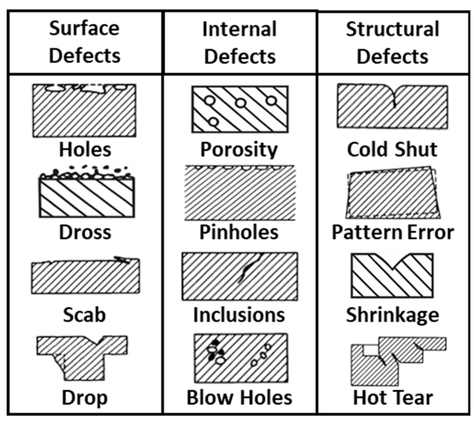
Figure 2.
Architecture of the proposed decision support system for multiclass defect classification.
Figure 2.
Architecture of the proposed decision support system for multiclass defect classification.
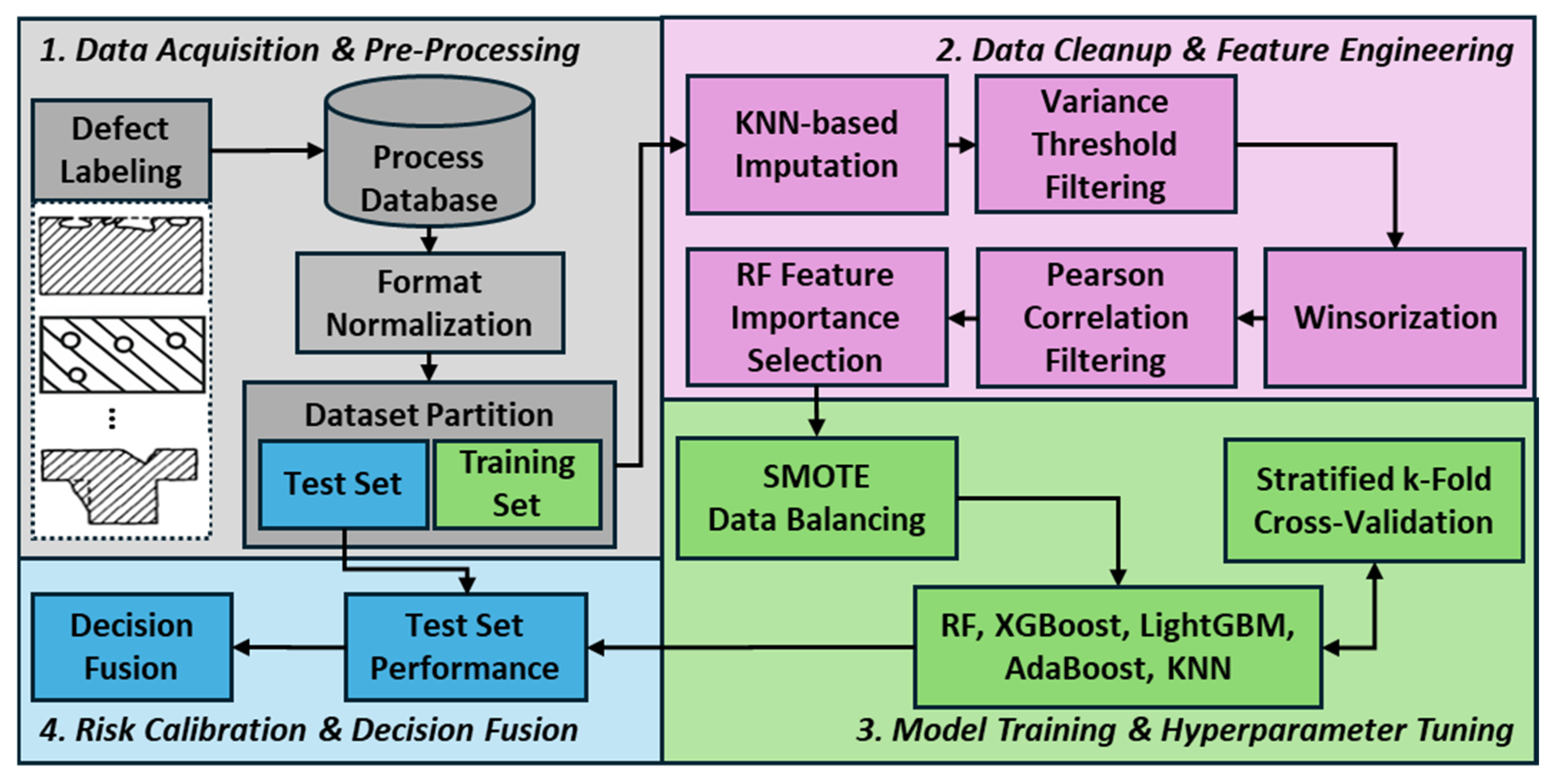
Figure 3.
Industrial dataset - database: exemplary errors I: missing data (red), skew data (blue), inconsistent units (pink).
Figure 3.
Industrial dataset - database: exemplary errors I: missing data (red), skew data (blue), inconsistent units (pink).
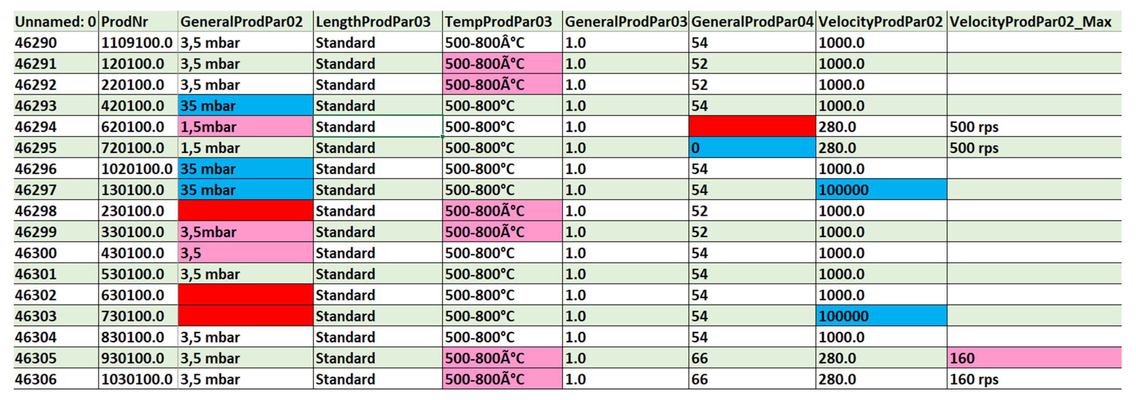
Figure 4.
Industrial dataset - database: exemplary errors II: duplicated entries (orange), faulty timestamps (grey), misaligned data (light brown).
Figure 4.
Industrial dataset - database: exemplary errors II: duplicated entries (orange), faulty timestamps (grey), misaligned data (light brown).

Figure 5.
Industrial dataset - exemplary excerpt of defect database.
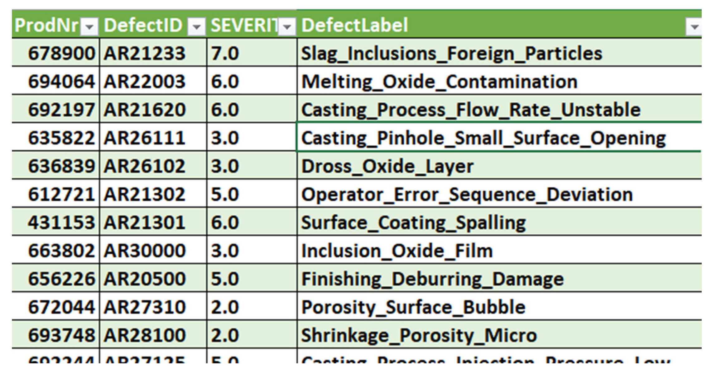
Figure 6.
Missingness Map - industrial database (df_main) – white: non-valid; black: valid.
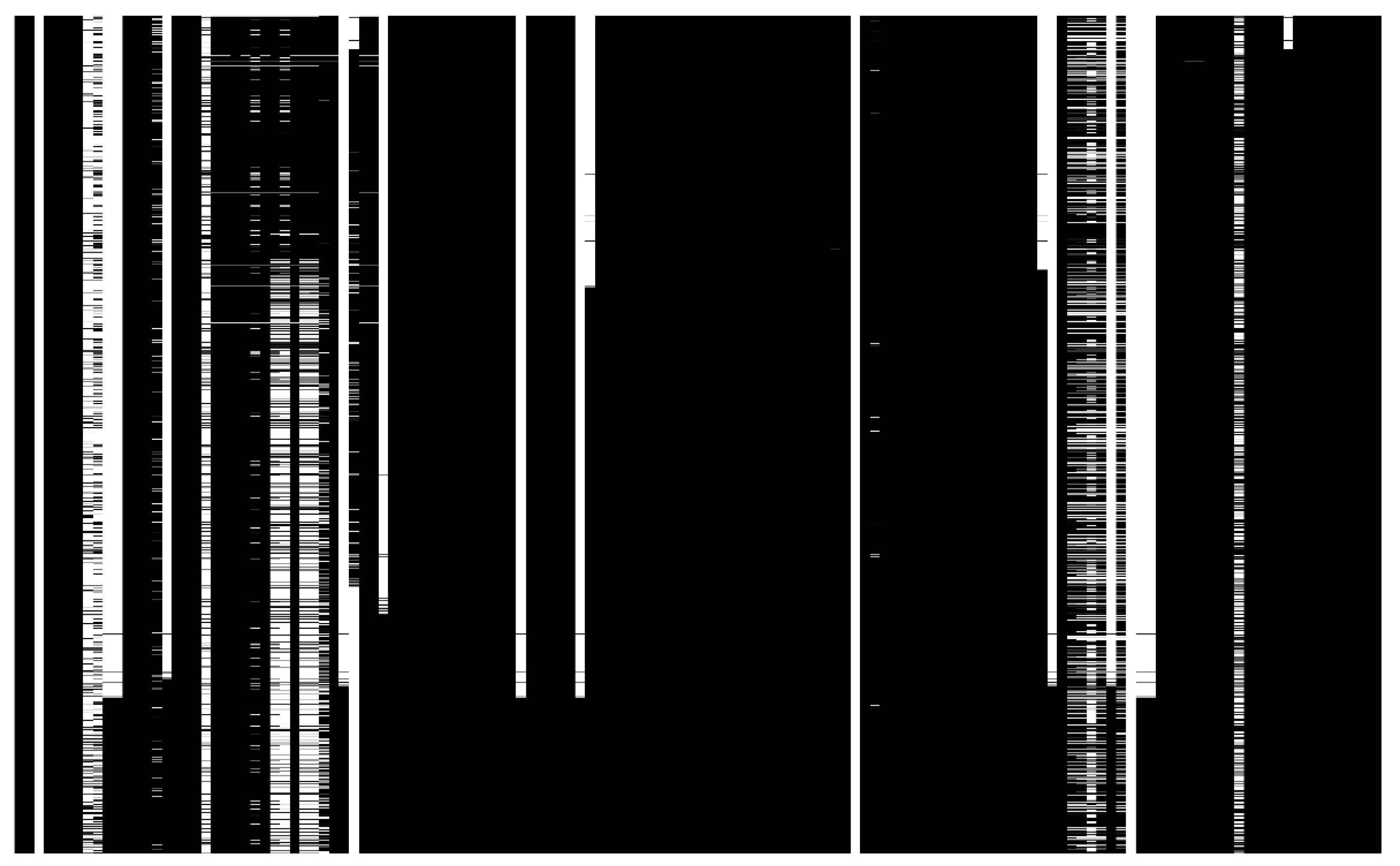
Figure 7.
Box-and-Whisker plots for five main outliers before Winsorization.
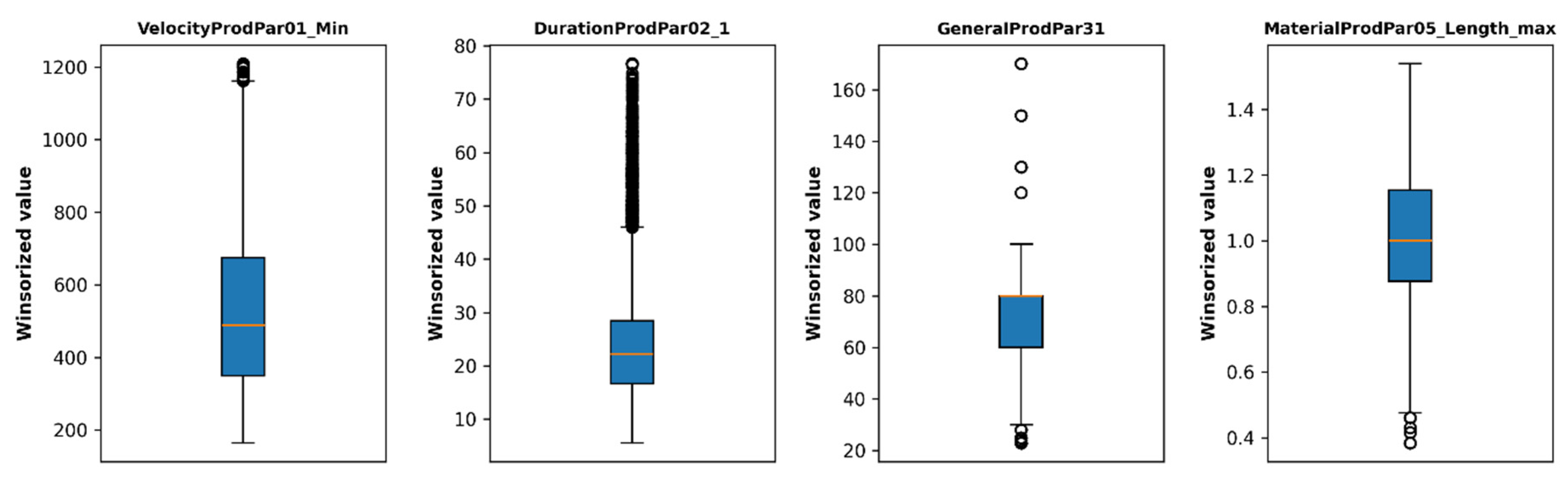
Figure 8.
Initial and Filtered production qualitative data correlation matrix; |r| = 0.995.
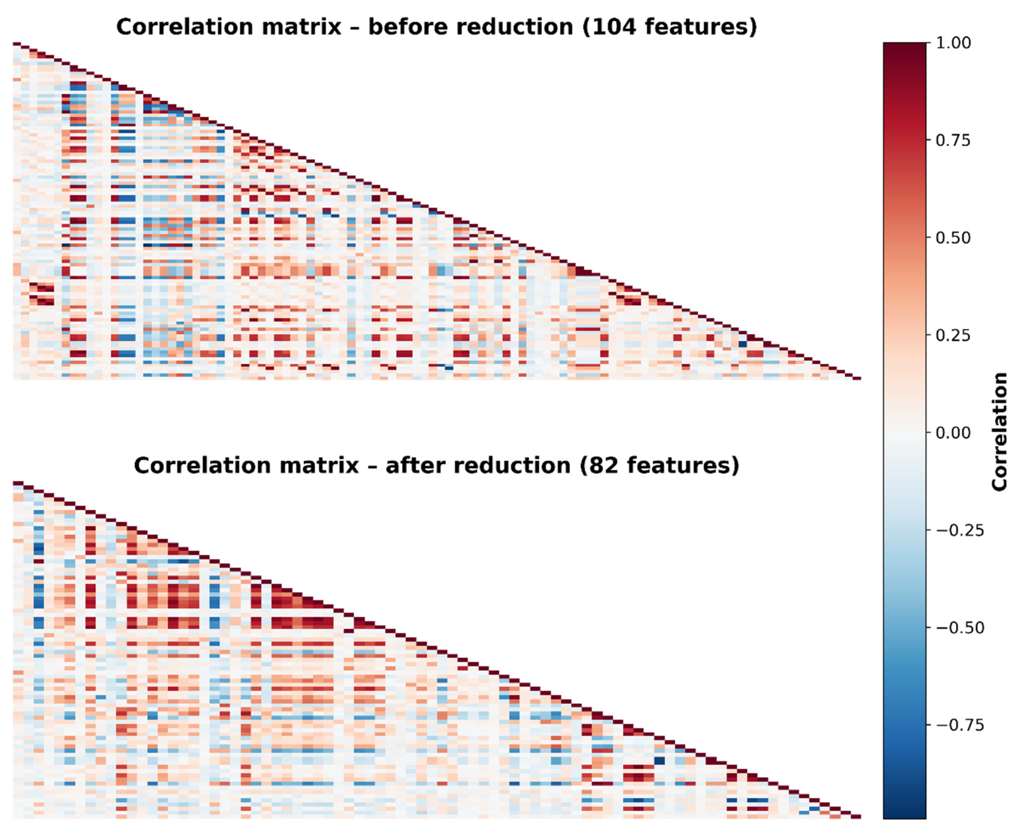
Figure 9.
Excerpt of 10 most (left) and least (right) important features (RFFI).
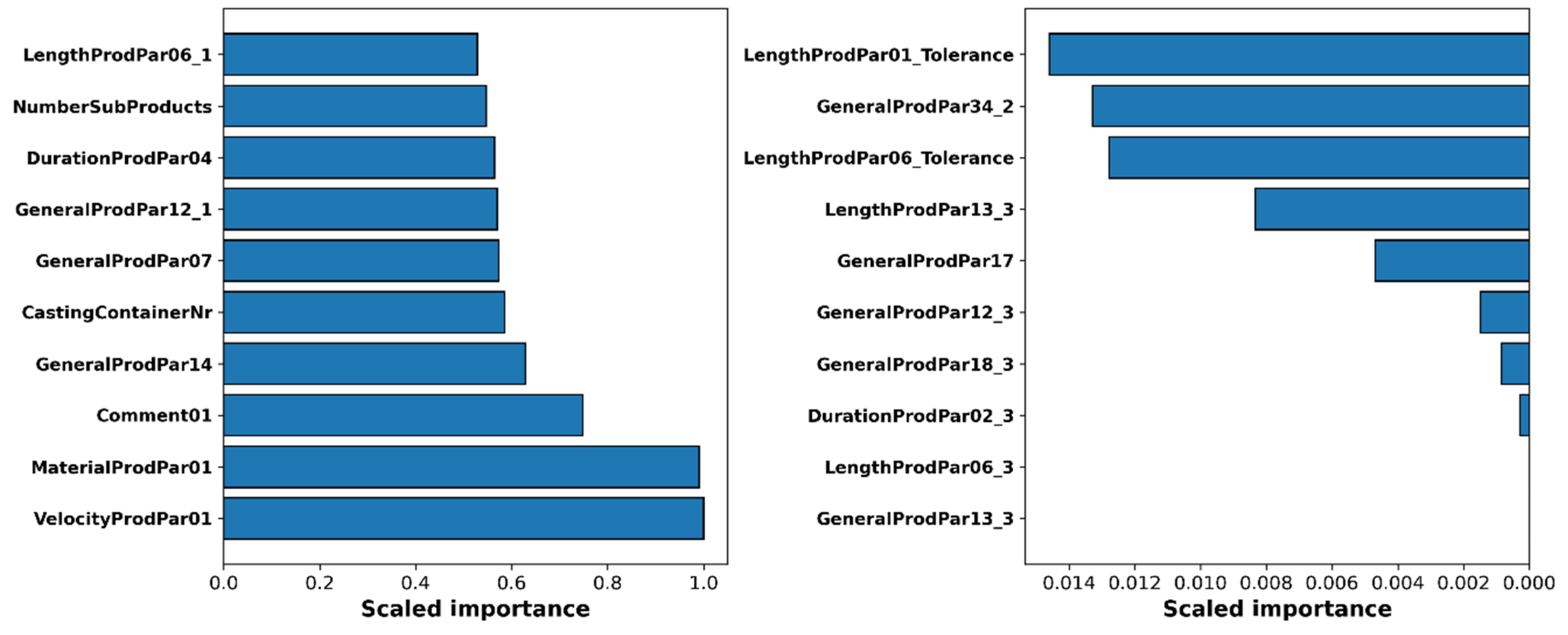
Figure 10.
Model-specific CV-results of macro
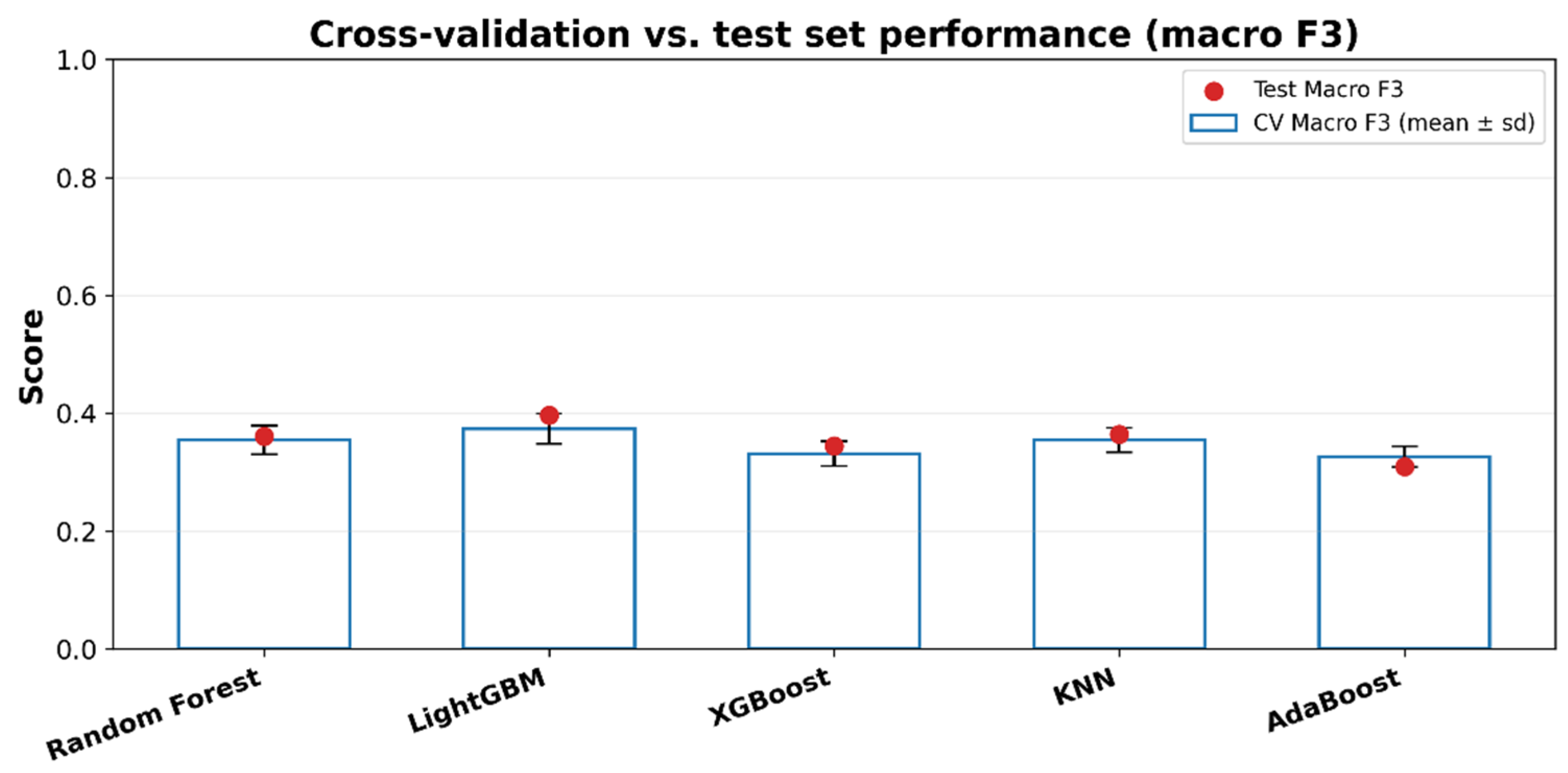
Figure 11.
Binary CM at the default maximum-probability threshold τCM = 0.5.
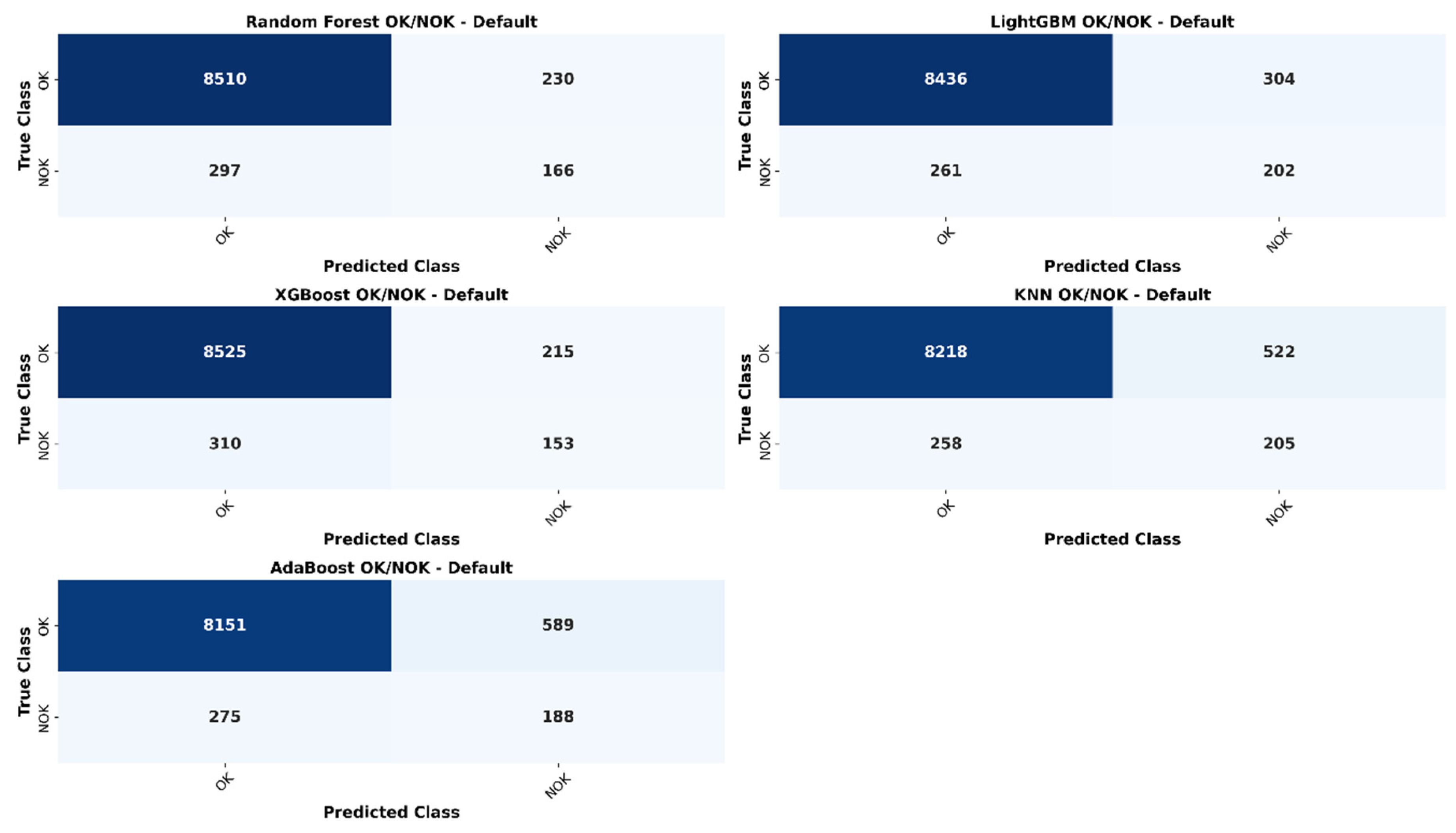
Figure 13.
Binary CM for decision fusion architectures at risk-calibrated thresholds.
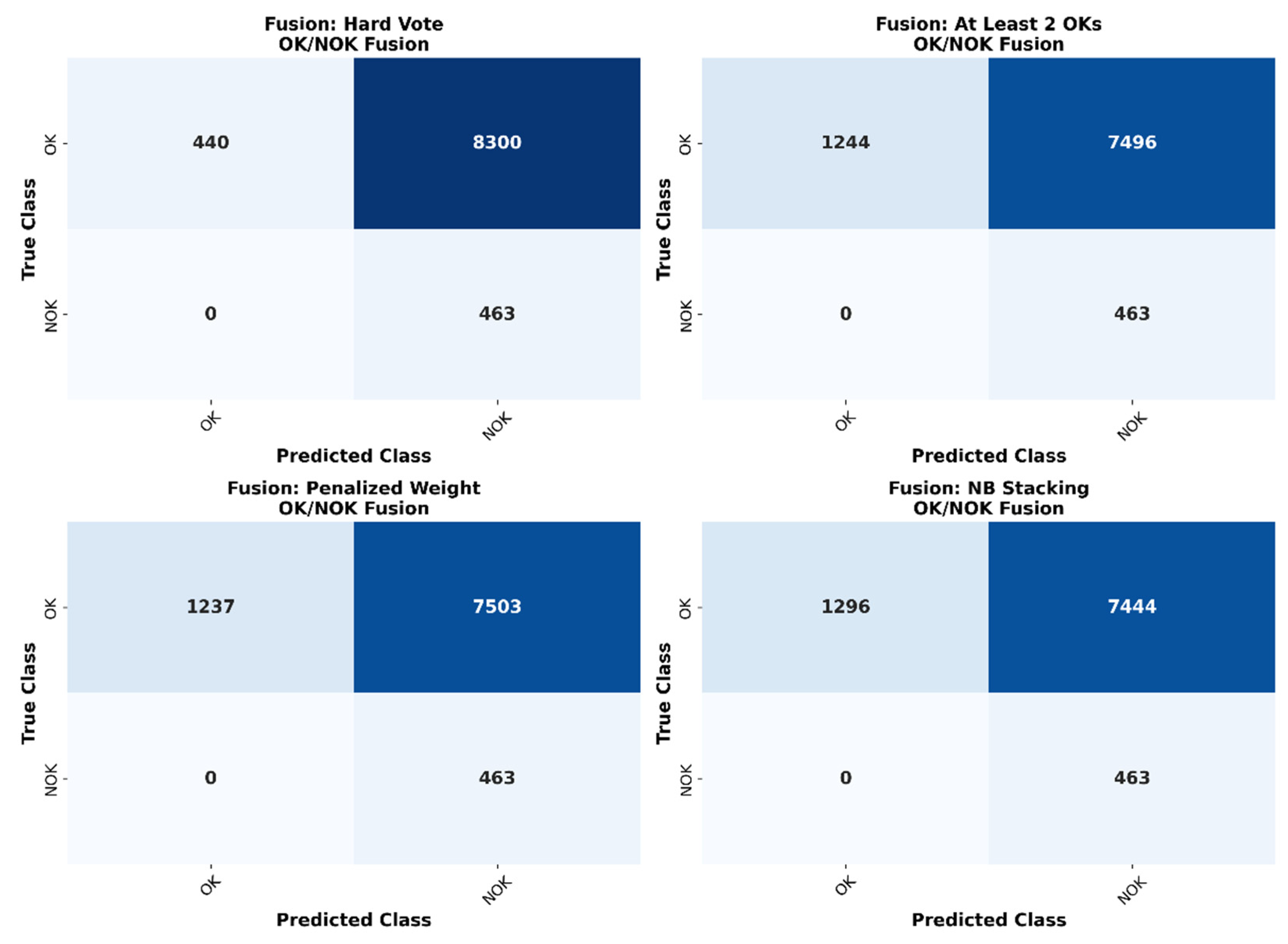

Table 1.
Hyperparameter Search Spaces and chosen classifier values.
| Model | Hyperparameter | Search Space | Chosen Value |
|---|---|---|---|
| RF |
n_estimators max_depth min_samples_split min_samples_leaf max_features class_weight |
200, 300, 500, 1000, 2000 10, 15, 20, 30, 40, 50, None 2, 4, 5, 6, 10 1, 2, 5 ‘sqrt’, ‘log2’, None ‘balanced’, ‘balanced_subsample’, None |
2000 20 4 2 ‘sqrt’ ‘balanced’ |
| kNN | n_neighbors weights metric |
3, 5, 7, 9, 10, 15 ‘uniform’, ‘distance’ ‘euclidean’, ‘manhattan’, ‘chebyshev’ |
15 ‘distance’ ‘manhattan’ |
| XGBoost |
learning_rate max_depth n_estimators subsample colsample_bytree min_child_weight gamma |
0.01, 0.05, 0.1, 0.2 3, 5, 7, 9, 10, 15 100, 200, 300, 500 0.6, 0.8, 1.0 0.6, 0.8, 1.0 1, 3, 5 0, 1, 5 |
0.01 7 500 0.8 1.0 1 5 |
| LightGBM | num_leaves max_depth learning_rate n_estimators min_child_samples class_weight |
15, 31, 63, 127, 255 5, 8, 12, 15, 20, 30, -1 0.01, 0.05, 0.1, 0.2 100, 200, 300, 500, 1000 10, 20, 40, 60 ‘balanced’, None |
63 30 0.01 1000 40 ‘balanced’ |
| AdaBoost | n_estimators learning_rate |
50, 100, 200, 300, 400 0.05, 0.1, 0.5, 0.7, 0.8, 1.0 |
200 0.5 |
Table 2.
Test set performance (macro-averaged metrics).
| Model | F3-score | Precision | Recall |
|---|---|---|---|
| RF | 0.361 | 0.378 | 0.360 |
| kNN | 0.364 | 0.300 | 0.376 |
| XGBoost | 0.344 | 0.382 | 0.343 |
| LightGBM | 0.397 | 0.375 | 0.400 |
| AdaBoost | 0.309 | 0.253 | 0.332 |
Disclaimer/Publisher’s Note: The statements, opinions and data contained in all publications are solely those of the individual author(s) and contributor(s) and not of MDPI and/or the editor(s). MDPI and/or the editor(s) disclaim responsibility for any injury to people or property resulting from any ideas, methods, instructions or products referred to in the content. |
© 2026 by the authors. Licensee MDPI, Basel, Switzerland. This article is an open access article distributed under the terms and conditions of the Creative Commons Attribution (CC BY) license.
Copyright: This open access article is published under a Creative Commons CC BY 4.0 license, which permit the free download, distribution, and reuse, provided that the author and preprint are cited in any reuse.


