

Submitted:
15 July 2026
Posted:
17 July 2026
You are already at the latest version
Abstract
Soybean is the main oilseed crop cultivated worldwide and is important for human and animal nutrition. The duration of flowering, reproductive period, and maturity is determined by genetic factors and influenced by environmental variables such as temperature, photoperiod, precipitation, soil type, and crop management, affecting yield and regional adaptation. However, gaps remain regarding the interaction between relative maturity groups (RMG) and the environment. Therefore, this study aimed to characterize the behavior of soybean populations and the environmental effect on the phenological cycle of the crop. Two populations were developed from biparental crosses with a narrow range in RMG among the parental cultivars. The E2 population originated from BMX Potência RR (RMG 6.7) × BMX Energia RR (RMG 5.3), and E3 from BRS 245 RR (RMG 7.3) × BRS 278 RR (RMG 9.4). The populations were evaluated over four growing seasons in an augmented block design, and traits were analyzed using mixed models with environmental covariates. Higher temperatures and lower precipitation were associated with shorter phenological periods, whereas higher precipitation and lower temperatures were associated with longer periods. Earlier lines were more environmentally sensitive, whereas later lines showed greater phenological stability.
Keywords:
environmental covariates
; Glycine max
; mixed models
; phenological cycle
; REML/BLUP
; genetic variability
1. Introduction
Soybean (Glycine max (L.) Merrill) is the main oilseed crop cultivated worldwide, with a major impact on protein and vegetable oil supply, being important for human and animal nutrition as well as bioenergy production [1]. In the 2025/2026 growing season in Brazil, soybean production is estimated at 180.13 million tons [2], maintaining the country as the world’s largest producer. Because of its economic importance and wide cultivation across diverse environments, agronomic traits related to the phenological cycle, such as number of days to flowering and maturity, have gained prominence in plant breeding programs. Genetic advances in soybean have been accompanied by changes in cycle duration, resulting in the development of more productive cultivars adapted to environmental conditions [3]. For this purpose, it is essential to classify cultivars according to their relative maturity group (RMG), allowing their proper allocation to different growing environments, since phenological maturity is strongly influenced by environmental factors such as latitude, altitude, and climate [4] in each region.
RMG is a widely used classification to describe the phenological cycle of soybean cultivars, based on plant responses to photoperiod and temperature, which are key regulatory factors for flowering and maturity [4]. The RMG system is an adaptation of the North American system, grouping genotypes into 13 classes (000, 00, 0, I, II, III, IV, V, VI, VII, VIII, IX, and X) representing adaptation ranges, from extremely early materials (group 000, high latitudes) to the latest ones (group X, latitude 0°) [5]. In Brazil, this classification was converted into a continuous numerical scale ranging from 5.0 (early cultivars) to 9.0 (late cultivars), facilitating regional cultivar placement and breeding cross planning [4]. In this context, RMG is also essential for defining sowing windows and suitable growing environments for each cultivar, since each adaptation zone is expected to meet the developmental requirements of specific maturity groups. However, when cultivars are grown outside the optimal sowing window or adaptation zone, their phenological cycle may be shortened or extended beyond the expected pattern [6].
From a biological perspective, this classification is associated with genetic differences underlying soybean phenological development. According to previous studies [7,8,9], genetic advances have enabled the identification of important loci and regulatory pathways associated with soybean flowering and maturity, including E-series genes, the J gene, circadian clock components, FT-like genes, and several QTLs. These loci influence the transition from vegetative to reproductive development, the duration of the reproductive period, and the time required to reach maturity. Thus, differences among genotypes in RMG represent not only agronomic variation, but also differences in the genetic control of phenology under different environmental conditions.
In addition to genetic factors inherent to each RMG, phenotypic expression is strongly influenced by environmental variables. In soybean, the main environmental effects related to changes in phenological behavior are temperature, photoperiod, and precipitation [10], as well as soil type and agricultural practices [11], also affecting yield and seed composition-related traits [12]. Considering these complex interactions, appropriate statistical methodologies are essential. Mixed models via REML/BLUP are particularly useful in plant breeding because they can handle unbalanced data, estimate variance components, predict genetic values with high accuracy, and incorporate environmental covariates into the analysis [13].
Despite these advances, there are still gaps in the understanding of soybean phenological behavior regarding the interaction between relative maturity groups and environmental variables. In this context, the objective of the present study was to: (i) characterize the response of soybean populations in terms of the duration of phenological periods across different growing seasons derived from crosses contrasting in RMG; (ii) select lines with high performance for yield and earliness using REML/BLUP in each population; and (iii) evaluate the effect of precipitation and temperature on the phenological cycle of these populations.
2. Materials and Methods
2.1. Experimental Area Characterization
The experiments were conducted at the Teaching, Research and Extension Farm (FEPE) of FCAV – UNESP, Jaboticabal Campus. The municipality is located in the northwestern region of the state of São Paulo, at latitude 21º 14’ 59” S and longitude 48º 17’ 8” W, at an altitude of 575 meters. The soil in the area is classified as a eutrophic dark-red Latosol, with a very clayey texture and gently undulating relief. According to the Köppen-Geiger classification, the climate of the region is type Cwa [14].
2.2. Genetic Material
Two populations were synthesized from narrow biparental crosses in relation to the Relative Maturity Group (RMG) of the cultivars used as parents. The combinations used to obtain the populations were as follows: BMX Potência RR (RMG 6.7) (♀) × BMX Energia RR (RMG 5.3) (♂), forming population E2, derived from parents with early and intermediate maturity cycles; and BRS 245 RR (RMG 7.3) (♀) × BRS 278 RR (RMG 9.4) (♂), forming population E3 [15], derived from parents with intermediate and late maturity cycles.
2.3. Experimental Design and Treatments
The experimental design used was an augmented block design [16], in which the lines (treatments) were arranged in single 5-meter rows, with 0.5 m spacing between rows (2.5 m² of useful area) and were included only once in the experiment without replication. Three check cultivars were interspersed within the blocks, each repeated twice per block, totaling 30 check plots across the five blocks. At least one of these checks consisted of one of the parental lines.
The checks used were: BMX Potência RR (6.7), AS 3680 IPRO (6.8), and M 6410 (6.4) for population E2; and BRS 245 RR (7.3), HO APORE IPRO (7.5), and BS 2606 IPRO (6.0) for population E3. The selection of checks was based on their maturity group proximity to that of the parental lines of the populations.
The populations were evaluated during the growing seasons 2020/2021, 2021/2022, 2022/2023, and 2023/2024. Population E2 (F7:10) consisted of 150 lines, while population E3 (F7:10) consisted of 80 lines, all at advanced generations of inbreeding.
2.4. Management of the Experimental Area
The management practices were carried out according to Embrapa recommendations [17]. The crops were established under a no-tillage system (NTS), with a sowing density of 18 plants per meter. Soil fertility was evaluated annually to ensure appropriate application of amendments and fertilizers. Seeds were inoculated with bacteria of the genus Bradyrhizobium to supply nitrogen. Pest, disease, and weed management were conducted as needed.
2.5. Evaluated Traits
2.5.1. Agronomic Traits
The evaluated traits were the number of days to flowering (NDF), number of reproductive days (NRD), number of days to maturity (NDM), and grain yield (GY). The NDF trait was assessed at the R1 phenological stage when plants transition from the vegetative to the reproductive phase. The NRD trait was calculated as the number of days from R1 to R8, and NDM was assessed at the R8 developmental stage, which corresponds to the period from sowing to the point when at least 50% of the plants have 95% or more mature pods, according to the classification of Fehr and Caviness [18] and is expressed in days. GY was obtained from the grain weight of the plot useful area (2.5 m²) after harvest and threshing. The data obtained in grams per plot were converted to kilograms per hectare (kg ha⁻¹) and adjusted to 13% moisture content.
2.5.2. Environmental Variables
In addition to the phenotypic evaluation of the traits, environmental variables associated with the lines were also assessed, namely accumulated precipitation (mm) and mean temperature (°C) during the cropping cycle. These variables were calculated individually for each line, considering the duration of each studied phenological period, to represent the climatic conditions experienced by each line throughout its development. This approach was adopted because fixed calendar windows could include periods in which earlier lines had already completed the evaluated phenological stage, potentially misrepresenting their environmental exposure. The meteorological data used in this study were provided by the Agroclimatological Station of the Department of Exact Sciences at FCAV/UNESP, Jaboticabal Campus.
2.6. Statistical Analyses
To visualize the behavior of NDF, NRD, NDM, and GY across growing seasons, boxplot graphs were used, as they allow comparison among cropping years, detection of patterns, and identification of differences related to line performance.
The linear mixed model used follows the structure presented by Bates et al. [19], defined by the conditional distribution of the response variable Y given the vector of random effects B:
where Xβ represents fixed effects, Zb random effects, σ² is the scale parameter (residual variance), and W is a diagonal matrix of known weights (assumed to be the identity).
For each experiment, the data were fitted using linear mixed models considering the structure of the Augmented Block Design (ABD), with genetic effects treated as random, using the lme4breeding package [20]. The model used was as follows:
where:
: observed value (NDM or GY)
: overall mean of the trait
: fixed effect of growing season : fixed effect of checks
: random effect of genotype : random effect of genotype x growing season interaction
: random effect of block
: experimental error.
The quality of the models was evaluated using the coefficient of determination (R²), with a decomposition of these coefficients into fixed and random effects, estimated using the rsq package. To assess the significance of fixed effects in the mixed model, a Wald-based ANOVA (Type III) was performed.
Residual diagnostics were performed for all fitted mixed models to assess normality and homogeneity of variance. For grain yield (GY), number of days to flowering (NDF), and number of reproductive days (NRD), residuals did not show relevant deviations from normality or homoscedasticity. For number of days to maturity (NDM), some deviation from these assumptions was observed; however, since variance components and fixed-effect estimates were obtained via restricted maximum likelihood (REML) within a linear mixed-model framework, which is comparatively robust to moderate departures from normality and homogeneity of variance, this deviation was not considered to materially compromise the reliability of the genetic parameter estimates or the significance tests reported for this trait.
The variance components (σg², σgxe², σe²) were estimated by restricted maximum likelihood (REML). The BLUPs (Best Linear Unbiased Predictors) were extracted from the estimated random effects in the mixed models. Two-dimensional scatter plots were generated between NDM and GY BLUPs to identify dual-purpose lines for earliness and higher productivity in each population.
The broad-sense heritability (H²) was estimated from the variance components for each population, considering the different years. According to the equation:
where a is the number of environments, corresponding to the evaluated growing seasons, and r is the number of within-environment replications. In the augmented block design used in this study, test lines were unreplicated within each growing season, therefore, r was considered equal to one for these lines. The replicated checks and blocks were used to adjust local environmental variation and improve experimental precision. The selective accuracy of the BLUPs was estimated as . To assess experimental precision, the experimental coefficient of variation was calculated, as well as the ratio between the genetic coefficient of variation and the experimental coefficient of variation .
Additionally, mixed models were fitted for NDF, NRD, and NDM, using environmental covariates as fixed effects to evaluate their influence on the phenotypic response of the populations, using the lme4 package [19]. Preliminary analyses indicated collinearity between accumulated precipitation and mean temperature, so these covariates were fitted in separate single-covariate models to avoid unstable coefficient estimates. In cases of low variation, the random block effect was not considered. The model used was as follows:
where:
: observed value (NDF, NRD and NDM)
: overall mean of the variable
: fixed effect of the environmental covariate (accumulated precipitation or mean temperature)
: fixed effect of checks
: random effect of the genotype x growing season interaction
: random effect of block
: experimental error.
Marginal prediction plots were generated, allowing visualization of the effect of environmental covariates on NDF, NRD, and NDM, using the ggeffects package. Model quality was evaluated using the coefficient of determination (R²), both marginal and conditional, estimated using the performance package, where marginal R² refers to the variance explained only by fixed effects and conditional R² represents the total variance explained by the model. The β coefficients were extracted from the fixed effects estimated by the mixed model. To assess the significance of fixed effects in the mixed model, a Wald-based ANOVA (Type III) was performed. All analyses and plots were generated using R software [21].
3. Results
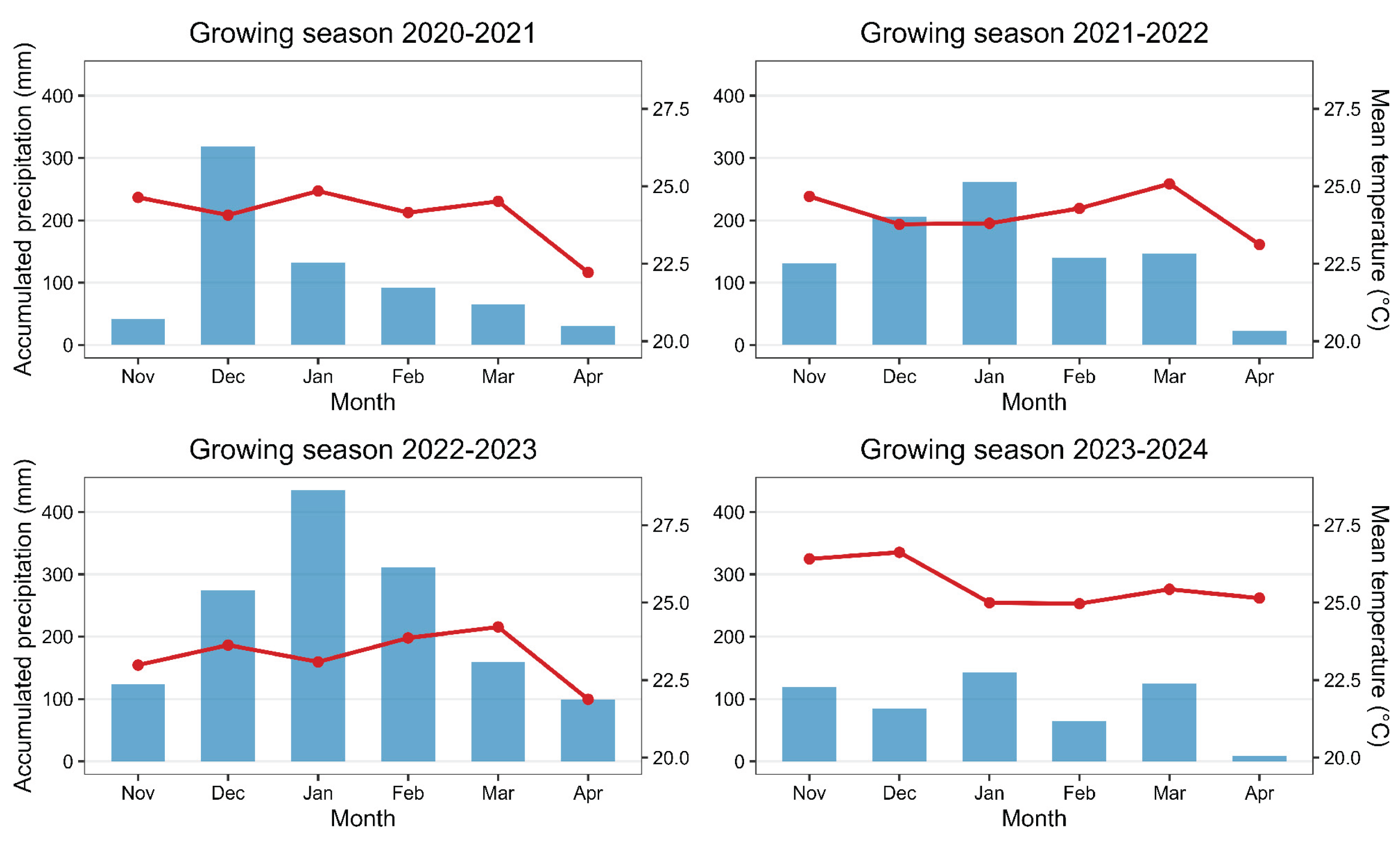
The distributions of accumulated precipitation (mm) and temperatures (°C) differed among the evaluated growing seasons. The 2020–2021 and 2021–2022 seasons showed similar temperature and precipitation patterns, whereas the 2022–2023 season was the coolest and had the highest rainfall intensity. In contrast, the 2023–2024 season presented the highest temperatures and the lowest precipitation levels (Figure A1).
The traits NDF, NRD, NDM, and GY of Population E2 exhibited different behaviors across the growing seasons (Figure 1). For NDF in Population E2, similar patterns were observed in the 2020-2021 and 2022-2023 seasons, with plants flowering within a similar range of days. In the 2021-2022 season, the plants exhibited delayed flowering, while in the 2023-2024 season, flowering occurred earlier. For NRD and NDM in Population E2, similar patterns to NDF were observed across all growing seasons, with the duration of the reproductive period and time to maturity showing consistent behavior across the different years. Regarding GY, a progressive decrease was observed across the growing seasons (Figure 1).
Population E3 exhibits later flowering compared to Population E2, in which the influence of the growing seasons on this trait is also observed. In the first three seasons, similar NDF patterns were noted, while in the 2023-2024 season, an earlier flowering can be observed (Figure 2). Regarding NRD, it can be observed that in the 2023-2024 season, when flowering occurred earlier, the number of reproductive days of the plants was higher than in previous seasons. The same NRD pattern can be observed in NDM. As in Population E2, GY in Population E3 showed a progressive decrease across the seasons (Figure 2).
For the population’s behavior, the growing season had a significant effect in all evaluated years, in some cases, the checks did not show a significant effect (Table 1). The coefficients of determination of each model were generally high, except for GY, with alternating importance between fixed and random effects across models. For NDF in populations E2 and E3, the variation was mostly accounted for by the fixed effects (0.65 and 0.76, respectively). For NRD, in population E2, the variation was also primarily due to the fixed effects (0.43), whereas in population E3, it was mainly attributable to the random effects (0.68). For NDM in populations E2 and E3, the random factors represented the main component of the variation (0.69 and 0.56, respectively). For GY, in the models for populations E2 and E3, the explanatory power was relatively low, but most of the variation was still due to the random effects (0.32 and 0.36, respectively) (Table 1).
In Population E2, the genotypic variance for NDF, NRD, and NDM was higher than the other variance components (2.65, 4.80, and 9.41, respectively), except for GY, which showed a high residual variance. The same pattern was observed in Population E3 for NDF, NRD, and NDM (10.21, 15.84, and 21.23), as well as a high residual variance for GY. The genotype × year interaction variance showed changes depending on the population and the trait analyzed, while the block variance was relatively low (Table 2).
NDF and NDM exhibited high heritabilities, NRD showed intermediate heritability, and GY presented lower heritability, especially in Population E3. The CVg/CVe ratio was greater than 1 for NDF, NRD, and NDM in both populations, indicating potential for selection on these traits, as well as the selective accuracy of the BLUPs. Regarding the means, Population E2 was characterized as earlier than Population E3 for both NDF and NDM. For NRD, Population E2 had a higher mean than Population E3. Concerning GY, Population E2 (3,553.15 kg ha⁻¹) showed better performance than Population E3 (2,953.71 kg ha⁻¹) (Table 2).
: genotypic variance; : genotype × year interaction variance; : variance of blocks within years; : residual variance; : broad-sense heritability; : selective accuracy of BLUPs; : experimental coefficient of variation; : genotypic coefficient of variation.
Figure 3 and Figure 4 show a dispersion of the BLUPs estimated for NDM and GY. The zero (0) point on the axes represents the overall mean for each trait. In this context, positive BLUPs for NDM indicate late lines, while negative BLUPs indicate early lines, based on the population mean. The same applies to GY, where lines with positive BLUPs are more productive and lines with negative BLUPs are less productive.
In Population E2 (Figure 3), BLUPs for NDM ranged from –10 to +5 days, representing a difference of 15 days between the earliest and latest lines. For GY, BLUPs ranged from –1089 to +700 kg ha⁻¹. A complete list of inbreed lines with their BLUP values for NDM and GY is provided in the Appendix A (Table A1).
For Population E3 (Figure 4), BLUPs for NDM ranged from –9 to +9 days, representing a difference of 18 days between the earliest and latest lines in the cycle. For GY, BLUPs ranged from –550 to +814 kg ha⁻¹. Full list of inbred lines is in Appendix A (Table A2).
To visualize the influence of the environment on the variation of NDF, NRD, and NDM, mixed models were fitted for each population using the environmental covariates accumulated precipitation and mean temperature. The models exhibited high explanatory power, with conditional R² ranging from 0.79 to 0.97 (Figure 5 and Figure 6).
The environmental covariates were significant (p < 0.001) in all models fitted for Population E2 (Table A3). Lower precipitation levels were associated with early flowering, while increased precipitation was associated with delayed flowering. The model exhibited high explanatory power (R² = 0.91), with a considerable contribution from accumulated precipitation (R² = 0.56), presenting a positive β coefficient, that is, for each 10 mm increase in precipitation, NDF increased by 0.42 days (Figure 5A, Table A3).
Lower temperatures are associated with delayed flowering, while higher temperatures are associated with earlier flowering. The model showed an explanatory power of 0.87, with mean temperature as a fixed effect explaining 0.30. The β coefficient was negative; that is, for each 1 °C increase in mean temperature, NDF decreases by 2.29 days (Figure 5B, Table A3).
Regarding NRD, the pattern is repeated: increased precipitation is associated with a higher number of reproductive days, while increased mean temperature is associated with a reduction in NRD. The models showed explanatory powers of 0.81 and 0.79, respectively, and a low contribution from the fixed effects (0.13 and 0.22, respectively), with a β coefficient of 0.052 for accumulated precipitation and –3.50 for mean temperature (Figure 5C–D, Table A3).
For NDM, that is, considering the entire cycle of the lines, the environmental covariates had significant effects, although their contributions were smaller than those of the random effects, with R² values of 0.18 for accumulated precipitation and 0.32 for mean temperature. The full models exhibited high explanatory power (0.94 and 0.93, respectively). For NDM, each 10 mm increase in precipitation resulted in an increase of 0.101 days in the total cycle, while each 1 °C increase led to a reduction of 5.56 days in the total cycle of the lines (Figure 5E–F, Table A3).
In Population E3, for NDF, increased precipitation delayed flowering of the lines, while increased temperature advanced flowering of the population. The models showed good fit, with conditional R² of 0.97 for accumulated precipitation and 0.96 for mean temperature, such that the fixed effects (0.65 and 0.68, respectively) were highly important in explaining the variation in flowering. The β coefficient was 0.169 for accumulated precipitation and –2.587 for mean temperature (Figure 6A–B, Table A3).
In contrast to what was observed for Population E2, regarding NRD, in Population E3 increased precipitation was associated with a shortening of the reproductive days, while increased temperature was associated with a prolongation of these days. The models showed high R² values (0.89 and 0.91, respectively), but with a low contribution from the fixed effects (0.11 and 0.21, respectively). The β coefficient was negative for precipitation (–0.068) and positive for mean temperature (4.867) (Figure 6C–D, Table A3).
For NDM, both models showed a conditional R² of 0.95. However, the fixed effects were not significant (p = 0.783 for accumulated precipitation and p = 0.726 for mean temperature), having no influence on the shortening or prolongation of the total cycle of the lines (Figure 6E–F, Table 3A). The decomposition of the coefficients of determination into fixed and random effects is available in the Appendix A (Table A4).
4. Discussion
The variability observed (Figure 1 and Figure 2) for NDF, NRD, NDM, and GY in the populations can be attributed to a combination of genetic and environmental factors: genetic factors associated with the maturity group (RMG) of each line and, consequently, adaptation to the location where the experiments were conducted; and environmental factors related to the climatic conditions of each growing season (Figure A1). Due to being a less contrasting cross in terms of RMG, population E2 presented lower genotypic variance for NDF, NRD, and NDM, characterizing a more early-maturing population, inheriting this trait from its parents. In contrast, population E3 showed higher genotypic variance for NDF, NRD, and NDM, largely due to the greater genetic distance between its parents (Table 2). This relationship between parental genetic distance and progeny variability was demonstrated by Jean et al. [22], as crosses between genetically distant parents generate a wide distribution of variance among the resulting progenies, whereas crosses between closely related parents generate lower variance among progenies for the trait in question.
Regarding the check cultivars, a significant effect (p < 0.001) was detected for NDF and NDM in population E3 (Table 1), whereas no significant check effect was observed in population E2 for any trait. This result likely reflects genetic differences among the three check cultivars used in population E3 (BRS 245 RR, HO APORE IPRO, and BS 2606 IPRO), which span a wider range of relative maturity groups (6.0 to 7.5) compared with the checks used in population E2. Because check performance was used to adjust for local environmental variation within blocks, this significant effect indicates that the checks captured genuine differences in phenological behavior rather than purely environmental noise, reinforcing the validity of using them as a reference for adjusting the BLUPs of the unreplicated test lines in this population.
The growing seasons had a strong influence on the phenological variables, as well as on GY of the populations, since in each growing season the same genotypes showed different performances (Figure 1 and Figure 2, Table 1, and Figure A1). This can be explained by the environmental conditions inherent to each growing season, which can affect plant phenological development as well as yield performance. Gong et al. [23] observed that changes in precipitation, temperature, and sunlight hours can shorten or extending the soybean phenological cycle. Soybean may exhibit positive or negative phenotypic plasticity depending on genotype × environment interaction. Generally, under stress conditions, as observed across seasons with reduced precipitation and increased temperature (Figure A1), plants may exhibit negative plasticity, reducing some traits such as yield components [24].
High broad-sense heritability estimates for NDF, ranging from 0.77 to 0.90 in both populations, demonstrate the strong genetic control of this trait, as also reported in the literature: 0.82 [25], 0.88 [26], and 0.94 [27]. In addition, flowering has a strong genetic component, although environmental heterogeneity is a crucial factor contributing to variation in flowering time in soybean [28], as also observed in our results. NRD in both populations showed intermediate heritability (0.68 and 0.66) and higher variance compared to NDF, demonstrating that the environment influences the duration of the reproductive phase, i.e., redistributing time among phases [29]. NDM (Table 2), ranging from 0.82 to 0.84, showed that despite environmental influence on the crop cycle, the genetic component plays a predominant role in the phenotypic expression of the trait, a fact widely reported in the literature. Previous studies have reported similar or higher heritability values, with estimates of 0.72 [26], 0.85 [30], 0.91 [31], 0.93 [32], and up to 0.94 [27].
For GY, the largest variance component observed was the residual, indicating that this trait is strongly influenced by environmental conditions [33] and other factors not included in the model, resulting in lower heritability values. Heritability estimates for GY were lower compared to phenological traits, ranging from 0.43 to 0.62 in both populations, which is expected for complex traits such as GY (Table 2). These results are consistent with values reported in other studies, which estimated heritability for yield at 0.59 [26] and 0.62 [30].
The use of mixed models through BLUPs in several breeding programs has proven to be an efficient tool for the prediction of genetic values and selection support, especially for quantitative traits influenced by the environment [34,35,36,37]. The distribution of BLUPs (Figure 3 and Figure 4) highlights the existence of genetic variability for NDM and GY within each population, which was also observed by Bianchi et al. [27]. This variability allows the identification and selection of lines with superior performance for earliness and productivity based on their predicted genetic value. Thus, as demonstrated in the present study, the BLUP-based approach enables the simultaneous selection of dual-purpose genotypes, considering phenological and productive traits in an integrated manner [38].
In population E2 (Figure 5A–F), accumulated precipitation showed a positive relationship, while mean temperature showed a negative relationship with the duration of phenological stages in both growing periods. In years with higher precipitation, an extension of the phenological cycle was observed, whereas drier years were associated with a reduction in cycle duration. Similarly, higher temperatures were associated with a shortening of the cycle, while cooler conditions resulted in longer duration. These results are consistent with the literature, which indicates that increased precipitation tends to prolong crop cycles, while increased temperature accelerates development and reduces the growth period [10,24,39]. This behavior is attributed to the fact that higher temperatures increase plant development rates, shortening phenological stages [40].
Liu and Dai [39], when evaluating the phenological response of soybean under different precipitation and temperature conditions, observed distinct effects depending on the developmental stage. In the vegetative period, variations of −0.01 to −0.11 days/10 mm of precipitation and −0.63 to −2.51 days/°C of mean temperature were reported. In the reproductive period, the effects ranged from −0.02 to 0.11 days/10 mm and −0.98 to 0.56 days/°C, indicating greater variability in the climatic response during this phase. For the total crop cycle, precipitation showed effects ranging from −0.06 to 0.09 days/10 mm, while temperature reduced the cycle duration by approximately 2.51 to 5.19 days/°C, depending on the region and growing season.
The β coefficients estimated in the present study for precipitation showed positive relationships with flowering (0.42 days/10 mm), reproductive period (0.052 days/10 mm), and maturity (0.101 days/10 mm), suggesting that increased precipitation tends to slightly prolong the duration of phenological stages. In contrast, mean temperature showed a consistent negative effect throughout the crop cycle, with a less pronounced reduction at flowering (−2.289 days/°C), followed by the reproductive period (−3.502 days/°C) and maturity (−5.565 days/°C), indicating that increased temperature progressively accelerates crop development (Figure 5A–F).
For population E3, the same pattern observed in population E2 for NDF was maintained regarding the effects of precipitation and temperature. For NRD, a shortening of the period was observed with increasing precipitation, and an extension of the period with increasing temperature, although the contribution of these variables was low (R² = 0.11 and 0.21, respectively; Figure 6C–D). This pattern is consistent with a possible self-compensation mechanism between phenological phases within the genotype itself; however, since no physiological measurements (e.g., photoassimilate partitioning or developmental rate at the sub-phase level) were taken in this study, this interpretation remains a hypothesis and warrants direct investigation in future research. For NDM, environmental covariates did not show a significant effect, suggesting that later-maturing genotypes are less sensitive to precipitation and temperature effects, maintaining a more stable phenological pattern across years (Figure 6A–F). This result is consistent with that reported by Sobko et al. [12], who found that early-maturing soybean genotypes are more sensitive to precipitation and temperature than later-maturing genotypes.
Both results obtained for populations E2 and E3 corroborate the study by Xin et al. [41], which demonstrates that soybean phenology is influenced by climatic conditions, with temperature generally exerting a negative effect on the duration of phenological stages, indicating an acceleration of crop development. And the precipitation shows a predominantly positive effect, being associated with the prolongation of phenological stages and the overall development cycle.
These results indicate that the inclusion of environmental variables in models becomes important for understanding how certain factors influence agronomic traits, allowing the quantification of specific effects on plant development. However, careful attention must be given to the selection of variables, as they should have a causal or physiological relationship with the process being modeled, and additionally environmental variables are generally collinear, which can make it difficult to distinguish the true contributions of different climatic factors [10].
Although this study provides relevant evidence on the effect of the environment on the phenological and productive modulation of biparental populations with contrasting maturity patterns, some limitations should be acknowledged. First, the experiments were conducted at a single location, although over four growing seasons. Therefore, although seasonal climatic variation was captured, the extrapolation of the results to other soybean-producing regions with different latitude, soil, altitude, and management conditions should be made with caution. Second, the study was based on only two biparental populations, which limits the generalization of the observed responses to the broader genetic diversity of soybean regarding relative maturity groups. Third, considering the large number of lines evaluated, the use of an augmented block design was an appropriate choice; however, this design did not allow replication of the lines within each growing season, which could have provided greater experimental precision.
An additional limitation concerns the plot structure used for grain yield estimation. Test lines were evaluated in single, unreplicated 5-m rows without border rows separating adjacent plots. While this configuration is commonly accepted for phenological traits such as NDF, NDM, and NRD, which are less susceptible to inter-plot interference and grain yield is known to be more sensitive to competition and border effects between neighboring plots, particularly in single-row, non-bordered designs. Shading, differential resource competition, and edge effects from adjacent genotypes with contrasting growth habits or maturity could have contributed to the high residual variance and comparatively low heritability observed for GY (Table 2), independently of genuine environmental effects. Therefore, part of the unexplained variance attributed to environmental influence may also reflect this methodological source of noise rather than climatic variation alone. Future evaluations aimed specifically at yield estimation would benefit from replicated plots with border rows or alternative spatial correction methods to better isolate genetic and environmental effects on this trait.
In addition, the environmental-covariate models focused on accumulated precipitation and mean temperature, although other factors relevant to the context of the study may also influence population responses, such as solar radiation, soil water availability, growing degree days, and biotic stresses. Environmental variables are often collinear, which may make it difficult to distinguish the true contributions of different climatic factors [10]. Because precipitation and temperature were evaluated separately due to collinearity, the estimated effects should be interpreted as associations with phenological responses, rather than as fully independent causal effects. Therefore, future studies including additional locations, greater genotype diversity with a broader range of RMG, and the use of replicated experimental designs would be useful to confirm the applicability of the results observed in this study.
5. Conclusions
Population E2 showed lower variability among lines and a predominance of early-maturing genotypes, characterized by uniformity, while population E3 also exhibited uniformity, but with predominantly late-maturing lines, resulting from parents that were not highly contrasting in terms of relative maturity group.
The use of mixed models via REML/BLUP was efficient for predicting genetic values and enabled the identification of lines with potentially higher productivity, as well as the identification of early-maturing lines.
Population E2 was more sensitive to environmental variations in precipitation and temperature, whereas population E3 showed a lower influence of these covariates on the lines cycle, suggesting that early-maturing genotypes exhibit greater phenotypic plasticity, while late-maturing genotypes tend to present greater phenological stability, compensating between vegetative and reproductive periods and resulting in a more stable total cycle duration.
Author Contributions
Conceptualization, E.F.B.A., S.H.U.-T., D.S.C. and L.F.A.; methodology, E.F.B.A., S.H.U.-T. and D.S.C.; validation, S.H.U.-T.; formal analysis, E.F.B.A. and F.M.F.; investigation, E.F.B.A., D.S.C., A.C.R.M., D.S.D.L., L.P.R., M.S.O. and J.S.S.; resources, S.H.U.-T. and L.F.A.; data curation, E.F.B.A. and D.S.C.; writing—original draft preparation, E.F.B.A.; writing—review and editing, E.F.B.A., S.H.U.-T. and G.V.M.; visualization, E.F.B.A.; supervision, S.H.U.-T.; project administration, S.H.U.-T.; funding acquisition, S.H.U.-T. All authors have read and agreed to the published version of the manuscript.
Funding
This study was financed in part by the Coordenação de Aperfeiçoamento de Pessoal de Nível Superior—Brasil (CAPES)—Finance Code 001.
Institutional Review Board Statement
Not applicable.
Informed Consent Statement
Not applicable.
Data Availability Statement
The data that support the findings of this study are available from the corresponding author upon request.
Acknowledgments
The authors are grateful to the Fazenda de Extensão, Pesquisa e Ensino (FEPE) for supporting the field experiments, and to the Agroclimatological Station of the Department of Exact Sciences for providing the meteorological data used in this study. Both institutions are affiliated with São Paulo State University (UNESP/FCAV). During the preparation of this manuscript, the authors used ChatGPT to review grammatical agreement and improve text fluency. The authors have reviewed and edited the output and take full responsibility for the content of this publication.
Conflicts of Interest
The authors declare no conflicts of interest.
Abbreviations
The following abbreviations are used in this manuscript:
| NDF | Number of days to flowering |
| NRD | Number of reproductive days |
| NDM | Number of days to maturity |
| GY | Grain Yield |
| RMG | Relative Maturity Group |
| REML | Restricted Maximum Likelihood |
| BLUP | Best Linear Unbiased Predictor |
Appendix A

Table A1.
Distribution of inbred lines according to BLUPs for number of days to maturity (NDM) and grain yield (GY) across four performance quadrants (Q1–Q4) for Population E2. Quadrants represent different agronomic profiles relative to the population mean: Q1 (below-average NDM and above-average yield), Q2 (below-average NDM and below-average yield), Q3 (above-average NDM and above-average yield), and Q4 (above-average NDM and below-average yield).
Table A1.
Distribution of inbred lines according to BLUPs for number of days to maturity (NDM) and grain yield (GY) across four performance quadrants (Q1–Q4) for Population E2. Quadrants represent different agronomic profiles relative to the population mean: Q1 (below-average NDM and above-average yield), Q2 (below-average NDM and below-average yield), Q3 (above-average NDM and above-average yield), and Q4 (above-average NDM and below-average yield).
| Quadrant | Agronomic class | Inbred line | BLUP NDM | BLUP yield |
| Q1 | Below-average NDM and above-average yield | POEN-58-108.1 | -0.08 | 614.89 |
| POEN-114-108.2 | -0.39 | 516.07 | ||
| POEN-35-147.3 | -1.44 | 476.39 | ||
| POEN-64-31.1 | -0.04 | 434.83 | ||
| POEN-81-183.1 | -0.26 | 406.19 | ||
| POEN-75-62.4 | -1.56 | 342.67 | ||
| POEN-95-166.2 | -0.25 | 296.41 | ||
| POEN-113-189.4 | -0.60 | 242.40 | ||
| POEN-18-114.4 | -1.41 | 224.09 | ||
| POEN-47-185.1 | -2.57 | 114.11 | ||
| POEN-63-116.1 | -0.46 | 89.18 | ||
| POEN-8-191.3 | -1.73 | 71.01 | ||
| POEN-60-183.4 | -0.47 | 68.26 | ||
| POEN-61-39.4 | -1.77 | 59.61 | ||
| POEN-6-192.2 | -1.56 | 18.93 | ||
| POEN-20-28.1 | -0.05 | 6.34 | ||
| Q2 | Below-average NDM and below-average yield | POEN-100-78.4 | -0.04 | -0.80 |
| POEN-23-191.2 | -6.23 | -10.40 | ||
| POEN-12-182.2 | -4.97 | -17.20 | ||
| POEN-13-70.3 | -6.48 | -41.76 | ||
| POEN-68-171.1 | -3.66 | -95.42 | ||
| POEN-46-120.1 | -3.50 | -103.85 | ||
| POEN-57-126.5 | -2.99 | -112.58 | ||
| POEN-77-40.3 | -0.47 | -121.00 | ||
| POEN-49-138.5 | -1.86 | -155.17 | ||
| POEN-27-192.4 | -1.39 | -167.11 | ||
| POEN-25-45.1 | -0.88 | -173.58 | ||
| POEN-48-45.3 | -0.08 | -180.65 | ||
| POEN-9-101.5 | -0.18 | -185.45 | ||
| POEN-55-182.1 | -1.86 | -194.25 | ||
| POEN-72-169.3 | -7.02 | -221.19 | ||
| POEN-34-118.1 | -3.50 | -241.47 | ||
| POEN-80-67.1 | -0.08 | -274.61 | ||
| POEN-14-124.2 | -6.60 | -277.43 | ||
| POEN-16-124.5 | -8.70 | -289.43 | ||
| POEN-19-24.4 | -2.02 | -295.17 | ||
| POEN-26-114.2 | -2.35 | -309.31 | ||
| POEN-94-30.1 | -0.05 | -309.41 | ||
| POEN-85-186.4 | -1.02 | -321.65 | ||
| POEN-65-192.1 | -2.57 | -353.34 | ||
| POEN-10-51.2 | -9.75 | -369.38 | ||
| POEN-59-179.1 | -1.39 | -377.73 | ||
| POEN-3-51.5 | -8.54 | -423.98 | ||
| POEN-32-45.2 | -0.81 | -430.21 | ||
| POEN-50-71.5 | -0.13 | -475.53 | ||
| POEN-93-61.5 | -0.26 | -481.41 | ||
| POEN-21-120.4 | -3.62 | -541.25 | ||
| POEN-15-92.3 | -1.23 | -606.44 | ||
| POEN-74-66.5 | -3.56 | -645.50 | ||
| POEN-2-51.4 | -8.25 | -653.22 | ||
| POEN-99-102.1 | -1.93 | -665.34 | ||
| POEN-28-192.5 | -0.71 | -677.12 | ||
| POEN-7-49.3 | -9.50 | -697.80 | ||
| POEN-5-49.5 | -6.36 | -787.89 | ||
| POEN-4-113.3 | -8.04 | -1089.65 | ||
| Q3 | Above-average NDM and above-average yield | POEN-71-196.2 | 2.81 | 700.00 |
| POEN-133-172.3 | 3.65 | 686.77 | ||
| POEN-107-104.2 | 3.02 | 681.42 | ||
| POEN-123-57.1 | 2.05 | 648.03 | ||
| POEN-104-143.4 | 2.35 | 593.72 | ||
| POEN-131-43.2 | 1.00 | 585.57 | ||
| POEN-136-115.5 | 1.72 | 567.76 | ||
| POEN-109-110.3 | 0.55 | 554.41 | ||
| POEN-150-199.1 | 2.47 | 507.76 | ||
| POEN-148-196.3 | 2.18 | 495.89 | ||
| POEN-79-183.3 | 1.00 | 488.86 | ||
| POEN-145-115.1 | 2.06 | 487.95 | ||
| POEN-86-29.1 | 1.42 | 474.16 | ||
| POEN-37-175.3 | 3.28 | 465.21 | ||
| POEN-121-10.3 | 0.55 | 450.17 | ||
| POEN-142-104.1 | 3.44 | 442.17 | ||
| POEN-126-188.1 | 1.72 | 436.65 | ||
| POEN-89-143.1 | 0.97 | 422.02 | ||
| POEN-84-43.3 | 1.97 | 414.21 | ||
| POEN-125-57.2 | 1.63 | 405.53 | ||
| POEN-17-108.3 | 1.08 | 356.17 | ||
| POEN-111-195.4 | 2.44 | 331.04 | ||
| POEN-24-3.5 | 0.50 | 319.25 | ||
| POEN-122-178.4 | 3.82 | 308.77 | ||
| POEN-56-14.5 | 2.18 | 274.17 | ||
| POEN-39-62.3 | 1.08 | 253.56 | ||
| POEN-118-119.3 | 0.97 | 253.38 | ||
| POEN-43-189.1 | 0.58 | 244.52 | ||
| POEN-22-103.1 | 2.23 | 240.18 | ||
| POEN-40-77.1 | 3.11 | 233.14 | ||
| POEN-45-66.1 | 0.38 | 226.40 | ||
| POEN-141-135.3 | 0.08 | 179.70 | ||
| POEN-116-178.2 | 2.44 | 168.51 | ||
| POEN-115-43.4 | 1.00 | 167.28 | ||
| POEN-120-43.5 | 0.71 | 166.35 | ||
| POEN-83-56.1 | 0.34 | 160.19 | ||
| POEN-103-194.1 | 1.01 | 155.59 | ||
| POEN-112-57.3 | 3.31 | 152.51 | ||
| POEN-54-125.5 | 0.38 | 147.07 | ||
| POEN-98-188.5 | 0.66 | 140.37 | ||
| POEN-91-176.3 | 1.93 | 137.37 | ||
| POEN-53-162.1 | 0.59 | 133.35 | ||
| POEN-51-32.1 | 1.60 | 132.38 | ||
| POEN-102-43.1 | 1.22 | 119.53 | ||
| POEN-108-178.1 | 0.97 | 116.67 | ||
| POEN-92-200.1 | 1.72 | 113.69 | ||
| POEN-144-195.3 | 1.64 | 111.87 | ||
| POEN-128-130.5 | 0.87 | 108.07 | ||
| POEN-82-176.4 | 1.42 | 105.27 | ||
| POEN-134-188.3 | 0.59 | 90.43 | ||
| POEN-42-52.2 | 4.45 | 81.96 | ||
| POEN-66-94.1 | 1.34 | 75.81 | ||
| POEN-101-149.1 | 0.17 | 69.96 | ||
| POEN-52-170.1 | 0.17 | 68.21 | ||
| POEN-138-57.4 | 1.81 | 65.15 | ||
| POEN-119-166.4 | 0.08 | 49.72 | ||
| POEN-87-186.3 | 0.50 | 43.65 | ||
| POEN-78-197.5 | 2.02 | 41.93 | ||
| POEN-110-71.1 | 2.06 | 41.27 | ||
| POEN-117-129.5 | 1.93 | 27.83 | ||
| POEN-67-165.5 | 2.06 | 21.11 | ||
| Q4 | Above-average NDM and below-average yield | POEN-130-103.2 | 0.79 | -8.00 |
| POEN-1-3.1 | 1.34 | -19.25 | ||
| POEN-139-153.1 | 0.87 | -22.15 | ||
| POEN-70-52.4 | 2.39 | -56.98 | ||
| POEN-146-178.5 | 3.02 | -72.86 | ||
| POEN-76-110.4 | 0.80 | -78.81 | ||
| POEN-90-30.3 | 0.34 | -80.53 | ||
| POEN-147-197.1 | 1.84 | -81.02 | ||
| POEN-38-14.3 | 0.24 | -89.06 | ||
| POEN-73-189.3 | 0.24 | -99.06 | ||
| POEN-33-113.2 | 2.35 | -108.28 | ||
| POEN-41-189.2 | 0.03 | -116.20 | ||
| POEN-96-141.2 | 1.00 | -117.51 | ||
| POEN-149-195.1 | 0.80 | -154.81 | ||
| POEN-132-195.5 | 0.38 | -162.58 | ||
| POEN-36-14.4 | 1.01 | -174.25 | ||
| POEN-62-29.3 | 1.97 | -193.76 | ||
| POEN-30-35.4 | 2.44 | -207.78 | ||
| POEN-129-35.5 | 2.18 | -222.85 | ||
| POEN-97-158.2 | 1.13 | -225.25 | ||
| POEN-135-188.2 | 2.89 | -237.59 | ||
| POEN-69-52.1 | 5.41 | -272.98 | ||
| POEN-11-78.1 | 0.97 | -287.62 | ||
| POEN-127-56.5 | 3.65 | -295.32 | ||
| POEN-124-103.3 | 2.06 | -305.39 | ||
| POEN-29-191.5 | 0.16 | -334.68 | ||
| POEN-31-29.5 | 1.81 | -334.92 | ||
| POEN-88-52.5 | 1.51 | -355.23 | ||
| POEN-140-179.2 | 1.84 | -384.26 | ||
| POEN-105-196.1 | 1.30 | -399.25 | ||
| POEN-44-191.4 | 0.38 | -411.12 | ||
| POEN-137-29.2 | 1.43 | -450.93 | ||
| POEN-106-30.5 | 1.13 | -483.05 | ||
| POEN-143-30.2 | 0.35 | -505.01 |
Table A2.
Distribution of inbred lines according to BLUPs for number of days to maturity (NDM) and grain yield (GY) across four performance quadrants (Q1–Q4) for Population E3. Quadrants represent different agronomic profiles relative to the population mean: Q1 (below-average NDM and above-average yield), Q2 (below-average NDM and below-average yield), Q3 (above-average NDM and above-average yield), and Q4 (above-average NDM and below-average yield).
Table A2.
Distribution of inbred lines according to BLUPs for number of days to maturity (NDM) and grain yield (GY) across four performance quadrants (Q1–Q4) for Population E3. Quadrants represent different agronomic profiles relative to the population mean: Q1 (below-average NDM and above-average yield), Q2 (below-average NDM and below-average yield), Q3 (above-average NDM and above-average yield), and Q4 (above-average NDM and below-average yield).
| Quadrant | Agronomic class | Inbred line | BLUP NDM | BLUP yield |
| Q1 | Below-average NDM and above-average yield | BR245BR278-5-42.1 | -0.76 | 557.68 |
| BR245BR278-55-3.2 | -2.41 | 295.51 | ||
| BR245BR278-34-68.5 | -4.97 | 294.62 | ||
| BR245BR278-45-3.1 | -3.64 | 262.57 | ||
| BR245BR278-48-68.3 | -1.60 | 257.00 | ||
| BR245BR278-49-75.4 | -4.67 | 227.94 | ||
| BR245BR278-47-38.5 | -3.85 | 211.53 | ||
| BR245BR278-2-71.3 | -4.84 | 152.49 | ||
| BR245BR278-7-69.3 | -4.15 | 147.49 | ||
| BR245BR278-69-41.3 | -1.79 | 143.87 | ||
| BR245BR278-53-4.3 | -0.98 | 136.90 | ||
| BR245BR278-9-10.3 | -6.83 | 136.05 | ||
| BR245BR278-10-42.3 | -2.20 | 130.72 | ||
| BR245BR278-59-53.3 | -0.57 | 129.41 | ||
| BR245BR278-30-38.3 | -3.65 | 100.22 | ||
| BR245BR278-26-23.2 | -2.00 | 77.73 | ||
| BR245BR278-4-11.5 | -9.22 | 77.60 | ||
| BR245BR278-13-20.4 | -5.59 | 77.41 | ||
| BR245BR278-51-34.5 | -0.14 | 77.26 | ||
| BR245BR278-20-6.5 | -5.80 | 73.96 | ||
| BR245BR278-18-71.1 | -2.63 | 60.67 | ||
| BR245BR278-40-9.1 | -1.17 | 51.99 | ||
| BR245BR278-29-11.1 | -6.53 | 22.36 | ||
| BR245BR278-17-3.4 | -5.87 | 15.84 | ||
| BR245BR278-68-5.4 | -1.26 | 7.93 | ||
| BR245BR278-41-16.1 | -3.87 | 2.74 | ||
| Q2 | Below-average NDM and below-average yield | BR245BR278-35-57.2 | -0.14 | -23.28 |
| BR245BR278-43-21.2 | -0.11 | -27.38 | ||
| BR245BR278-46-41.2 | -3.44 | -34.05 | ||
| BR245BR278-24-3.3 | -5.67 | -45.41 | ||
| BR245BR278-3-69.1 | -5.18 | -51.23 | ||
| BR245BR278-11-23.1 | -0.16 | -53.93 | ||
| BR245BR278-63-41.4 | -2.17 | -97.72 | ||
| BR245BR278-25-29.2 | -3.32 | -102.79 | ||
| BR245BR278-79-68.1 | -0.44 | -113.89 | ||
| BR245BR278-44-16.2 | -2.71 | -131.97 | ||
| BR245BR278-74-3.5 | -2.00 | -174.92 | ||
| BR245BR278-28-1.2 | -1.58 | -205.86 | ||
| BR245BR278-15-71.2 | -1.60 | -207.21 | ||
| BR245BR278-39-5.2 | -1.39 | -208.12 | ||
| BR245BR278-8-24.2 | -1.79 | -233.56 | ||
| BR245BR278-32-47.1 | -1.39 | -294.47 | ||
| BR245BR278-6-11.2 | -9.30 | -474.50 | ||
| Q3 | Above-average NDM and above-average yield | BR245BR278-37-38.4 | 2.74 | 814.48 |
| BR245BR278-33-68.4 | 2.57 | 247.65 | ||
| BR245BR278-21-21.3 | 1.34 | 245.60 | ||
| BR245BR278-70-17.3 | 4.22 | 202.89 | ||
| BR245BR278-65-41.5 | 0.48 | 185.24 | ||
| BR245BR278-19-23.4 | 0.27 | 148.61 | ||
| BR245BR278-62-12.1 | 5.42 | 135.60 | ||
| BR245BR278-27-17.1 | 1.34 | 120.26 | ||
| BR245BR278-16-34.3 | 1.75 | 114.26 | ||
| BR245BR278-60-55.3 | 5.53 | 110.87 | ||
| BR245BR278-73-52.3 | 0.67 | 89.97 | ||
| BR245BR278-22-21.4 | 0.68 | 87.77 | ||
| BR245BR278-61-14.5 | 0.87 | 71.96 | ||
| BR245BR278-57-74.5 | 9.33 | 48.59 | ||
| BR245BR278-12-15.2 | 6.77 | 44.35 | ||
| BR245BR278-52-6.2 | 1.09 | 25.15 | ||
| BR245BR278-78-52.2 | 7.48 | 24.33 | ||
| BR245BR278-66-74.1 | 1.75 | 23.79 | ||
| Q4 | Above-average NDM and below-average yield | BR245BR278-54-12.4 | 3.56 | -17.33 |
| BR245BR278-31-17.4 | 2.65 | -64.08 | ||
| BR245BR278-72-74.2 | 1.49 | -76.13 | ||
| BR245BR278-42-6.1 | 0.47 | -115.58 | ||
| BR245BR278-38-38.2 | 3.57 | -121.12 | ||
| BR245BR278-77-74.4 | 6.28 | -124.90 | ||
| BR245BR278-1-57.1 | 6.23 | -151.66 | ||
| BR245BR278-67-57.4 | 5.04 | -162.25 | ||
| BR245BR278-23-59.3 | 2.52 | -164.92 | ||
| BR245BR278-14-23.5 | 1.54 | -175.10 | ||
| BR245BR278-36-1.1 | 2.93 | -183.58 | ||
| BR245BR278-76-35.5 | 4.92 | -222.91 | ||
| BR245BR278-75-52.4 | 5.22 | -233.62 | ||
| BR245BR278-58-10.1 | 8.63 | -263.20 | ||
| BR245BR278-50-12.3 | 4.84 | -277.13 | ||
| BR245BR278-64-34.1 | 0.88 | -288.74 | ||
| BR245BR278-56-57.3 | 3.60 | -309.09 | ||
| BR245BR278-71-35.1 | 5.01 | -488.37 | ||
| BR245BR278-80-55.5 | 9.74 | -550.85 |
Table A3.
Coefficients of determination (R²) and results of the type III Wald test for fixed effects in the mixed models fitted for NDF, NRD, and NDM in two soybean populations, considering two environmental covariates: accumulated precipitation and mean temperature. Jaboticabal, SP.
Table A3.
Coefficients of determination (R²) and results of the type III Wald test for fixed effects in the mixed models fitted for NDF, NRD, and NDM in two soybean populations, considering two environmental covariates: accumulated precipitation and mean temperature. Jaboticabal, SP.
| Population | Trait | Environmental covariate | Conditional R² | Marginal R² | β coefficient | χ² | p-value | n |
| E2 | NDF | Accumulated precipitation | 0.91 | 0.56 | 0.420 | 838.47 | < 0.001*** | 718 |
| Mean temperature | 0.87 | 0.30 | -2.289 | 260.26 | < 0.001*** | |||
| NRD | Accumulated precipitation | 0.81 | 0.13 | 0.052 | 65.74 | < 0.001*** | 717 | |
| Mean temperature | 0.79 | 0.22 | -3.502 | 142.92 | < 0.001*** | |||
| NDM | Accumulated precipitation | 0.94 | 0.18 | 0.101 | 126.58 | < 0.001*** | 717 | |
| Mean temperature | 0.93 | 0.32 | -5.565 | 277.33 | < 0.001*** | |||
| E3 | NDF | Accumulated precipitation | 0.97 | 0.65 | 0.169 | 120.75 | < 0.001*** | 439 |
| Mean temperature | 0.96 | 0.68 | -2.587 | 139.57 | < 0.001*** | |||
| NRD | Accumulated precipitation | 0.89 | 0.11 | -0.068 | 11.44 | < 0.001*** | 439 | |
| Mean temperature | 0.91 | 0.21 | 4.867 | 52.77 | < 0.001*** | |||
| NDM | Accumulated precipitation | 0.96 | 0.35 | -0.004 | 0.08 | 0.783 ns | 439 | |
| Mean temperature | 0.96 | 0.35 | -0.203 | 0.12 | 0.726 ns |
χ²: Chi-square; p-value: significance of fixed effects in each experiment; NDF: number days to flowering; NRD: number of reproductive days; NDM: number of days to maturity; n: represents the number of observations used to fit each covariate model after removing missing values. Conditional and marginal R² values were estimated using the performance package. β coefficients were extracted from the fixed-effect estimates of the mixed models. p-values refer to type III Wald tests for the environmental covariates. Significance codes: *** p ≤ 0.001; ** p ≤ 0.01; * p ≤ 0.05; p ≤ 0.1; ns: not significant (p > 0.1).
Table A4.
Decomposition of the coefficient of determination into fixed and random effects in mixed models fitted for phenological traits in two soybean populations. Jaboticabal, SP.
Table A4.
Decomposition of the coefficient of determination into fixed and random effects in mixed models fitted for phenological traits in two soybean populations. Jaboticabal, SP.
| Population | Trait | Environmental covariate | Model R² | Fixed R² | Random R² |
| E2 | NDF | Accumulated precipitation | 0.910 | 0.563 | 0.347 |
| Mean temperature | 0.867 | 0.301 | 0.566 | ||
| NRD | Accumulated precipitation | 0.796 | 0.127 | 0.669 | |
| Mean temperature | 0.777 | 0.230 | 0.547 | ||
| NDM | Accumulated precipitation | 0.930 | 0.183 | 0.746 | |
| Mean temperature | 0.921 | 0.340 | 0.581 | ||
| E3 | NDF | Accumulated precipitation | 0.965 | 0.672 | 0.293 |
| Mean temperature | 0.957 | 0.704 | 0.254 | ||
| NRD | Accumulated precipitation | 0.876 | 0.105 | 0.771 | |
| Mean temperature | 0.885 | 0.088 | 0.797 | ||
| NDM | Accumulated precipitation | 0.950 | 0.380 | 0.571 | |
| Mean temperature | 0.950 | 0.384 | 0.566 |
Model R², Fixed R² and Random R² were obtained using the rsq package. NDF: number of days to flowering; NRD: number of reproductive days; NDM: number of days to maturity.
Appendix B
Figure A1.
Climogram of monthly accumulated precipitation (mm) and mean temperature (°C) during the evaluated growing seasons.
Figure A1.
Climogram of monthly accumulated precipitation (mm) and mean temperature (°C) during the evaluated growing seasons.
References
- Pagano, M.C.; Miransari, M. The importance of soybean production worldwide. In Abiotic and Biotic Stresses in Soybean Production: Soybean Production; Miransari, M., Ed.; Academic Press: Cambridge, MA, USA, 2016; pp. 1–26. [Google Scholar] [CrossRef]
- CONAB. Produção de grãos deve atingir 358,6 milhões de toneladas na safra 2025/26 . Available online: https://www.gov.br/conab/pt-br/assuntos/noticias/producao-de-graos-deve-atingir-358-6-milhoes-de-toneladas-na-safra-2025-26 (accessed on 12 June 2026).
- Todeschini, M.H.; Milioli, A.S.; Rosa, A.C.; Dallacorte, L.V.; Panho, M.C.; Marchese, J.A.; Benin, G. Soybean genetic progress in South Brazil: physiological, phenological and agronomic traits. Euphytica 2019, 215, 124. [Google Scholar] [CrossRef]
- Alliprandini, L.F.; Abatti, C.; Bertagnolli, P.F.; Cavassim, J.E.; Gabe, H.L.; Kurek, A.; Matsumoto, M.N.; de Oliveira, M.A.R.; Pitol, C.; Prado, L.C.; Steckling, C. Understanding soybean maturity groups in Brazil: environment, cultivar classification, and stability. Crop Sci. 2009, 49, 801–808. [Google Scholar] [CrossRef]
- Heatherly, L.G.; Elmore, R.W. Managing inputs for peak production. In Soybeans: Improvement, Production and Uses, 3rd ed.; Boerma, H.R., Specht, J.E., Eds.; American Society of Agronomy: Madison, WI, USA, 2004; pp. 451–536. [Google Scholar]
- Bubans, V.E.; Carvalho, I.R.; Ceolin, C.; Moura, N.B.; Lautenchleger, F.; Conceição, G.M.; Da Silva, J.A.G.; Treter, R.J. Relative maturity group and its relationships with the non-preferential sowing season in soybean. Agron. Sci. Biotechnol. 2021, 7, 1–14. [Google Scholar] [CrossRef]
- Lin, X.; Liu, B.; Weller, J.L.; Abe, J.; Kong, F. Molecular mechanisms for the photoperiodic regulation of flowering in soybean. J. Integr. Plant Biol. 2021, 63, 981–994. [Google Scholar] [CrossRef] [PubMed]
- Lin, X.; Dong, L.; Tang, Y.; Li, H.; Cheng, Q.; Li, H.; Zhang, T.; Ma, L.; Xiang, H.; Chen, L.; Nan, H.; Fang, C.; Lu, S.; Li, J.; Liu, B.; Kong, F. Novel and multifaceted regulations of photoperiodic flowering by phytochrome A in soybean. Proc. Natl. Acad. Sci. USA 2022, 119, e2208708119. [Google Scholar] [CrossRef] [PubMed]
- Wang, F.; Han, T.; Chen, Z.J. Circadian and photoperiodic regulation of the vegetative to reproductive transition in plants. Commun. Biol. 2024, 7, 579. [Google Scholar] [CrossRef] [PubMed]
- He, L.; Jin, N.; Yu, Q. Impacts of climate change and crop management practices on soybean phenology changes in China. Sci. Total Environ. 2020, 707, 135638. [Google Scholar] [CrossRef] [PubMed]
- Romeiko, X.X.; Lee, E.K.; Sorunmu, Y.; Zhang, X. Spatially and temporally explicit life cycle environmental impacts of soybean production in the U.S. Midwest. Environ. Sci. Technol. 2020, 54, 4758–4768. [Google Scholar] [CrossRef] [PubMed]
- Sobko, O.; Stahl, A.; Hahn, V.; Zikeli, S.; Claupein, W.; Gruber, S. Environmental effects on soybean (Glycine max (L.) Merr.) production in Central and South Germany. Agronomy 2020, 10, 1847. [Google Scholar] [CrossRef]
- Resende, M.D.V. Software Selegen-REML/BLUP: a useful tool for plant breeding. Crop Breed. Appl. Biotechnol. 2016, 16, 330–339. [Google Scholar] [CrossRef]
- Lima, R.F.; Aparecido, L.E.O.; Torsoni, G.B.; Rolim, G.S. Climate change assessment in Brazil: utilizing the Köppen-Geiger (1936) climate classification. Rev. Bras. De Meteorol. 2023, 38, e38230001. [Google Scholar] [CrossRef]
- Amaral, L.O.; Miranda, G.V.; Val, B.H.P.; Silva, A.P.; Moitinho, A.C.R.; Unêda-Trevisoli, S.H. Artificial neural network for discrimination and classification of tropical soybean genotypes of different relative maturity groups. Front. Plant Sci. 2022, 13, 814046. [Google Scholar] [CrossRef] [PubMed]
- Federer, W.T. Augmented (or hoonuiaku) designs. Hawaii. Plant. Rec. 1956, 55, 191–208. [Google Scholar]
- Seixas, C.D.S.; Neumaier, N.; Balbinot Junior, A.A.; Krzyzanowski, F.C.; Leite, R.M.V.C. (Eds.) Tecnologias de Produção de Soja . In Série Sistemas de Produção; Embrapa Soja: Londrina, Brazil, 2020; Volume No. 17, p. 347p. [Google Scholar]
- Fehr, W.R.; Caviness, C.E. Stages of Soybean Development; Iowa State University of Science and Technology: Ames, IA, USA, 1977; Volume 11p. [Google Scholar]
- Bates, D.; Mächler, M.; Bolker, B.M.; Walker, S.C. Fitting linear mixed-effects models using lme4. J. Stat. Software. 2015, 67, 1–48. [Google Scholar] [CrossRef]
- Covarrubias-Pazaran, G. lme4breeding: Relationship-Based Mixed-Effects Models, version 1.0.63; CRAN: Vienna, Austria, 2025. [Google Scholar]
- R Core Team. R: A Language and Environment for Statistical Computing; R Foundation for Statistical Computing: Vienna, Austria, 2024; Available online: https://www.R-project.org/.
- Jean, M.; Cober, E.; O’Donoughue, L.; Rajcan, I.; Belzile, F. Improvement of key agronomical traits in soybean through genomic prediction of superior crosses. Crop Sci. 2021, 61, 3908–3918. [Google Scholar] [CrossRef]
- Gong, L.; Tian, B.; Li, Y.; Wu, S. Phenological changes of soybean in response to climate conditions in frigid region in China over the past decades. Int. J. Plant Prod. 2021, 15, 363–375. [Google Scholar] [CrossRef]
- Poudel, S.; Adhikari, B.; Dhillon, J.; Reddy, K.R.; Stetina, S.R.; Bheemanahalli, R. Quantifying the physiological, yield, and quality plasticity of southern USA soybeans under heat stress. Plant Stress. 2023, 9, 100195. [Google Scholar] [CrossRef]
- Kuswantoro, H.; Artari, R.; Rahajeng, W.; Ginting, E.; Supeno, A. Genetic variability, heritability, and correlation of some agronomical characters of soybean varieties. Biosaintifika 2018, 10, 9–15. [Google Scholar] [CrossRef]
- Sulistyo, A.; Purwantoro; Sari, K.P. Correlation, path analysis and heritability estimation for agronomic traits contribute to yield on soybean. IOP Conf. Ser. Earth Environ. Sci. 2018, 102, 012034. [Google Scholar] [CrossRef]
- Bianchi, M.C.; Bruzi, A.T.; Soares, I.O.; Ribeiro, F.D.O.; Gesteira, G.D.S. Heritability and the genotype × environment interaction in soybean. Agrosystems Geosci. Environ. 2020, 3, e20020. [Google Scholar] [CrossRef]
- Xiong, G.; Wang, L.; Naser, M.; Zhao, M.; Chen, J.; Jiang, B.; Yuan, S.; Qin, C.; Han, T.; Sun, S.; Wu, T. Genetic and environmental determinants underlying the dynamics of soybean flowering time. Plant Cell Environ. 2025, 49, 4524–4543. [Google Scholar] [CrossRef] [PubMed]
- Kumudini, S.V.; Pallikonda, P.K.; Steele, C. Photoperiod and E-genes influence the duration of the reproductive phase in soybean. Crop Sci. 2007, 47, 1510–1517. [Google Scholar] [CrossRef]
- Teixeira, F.G.; Hamawaki, O.T.; Nogueira, A.P.O.; Hamawaki, R.L.; Hamawaki, C.L.; Mattos, T.P.; Silveira, I.C.; Medeiros, L.A. Inheritance of precocity and of agronomic characters in soybean. Genet. Mol. Res. 2017, 16, gmr16039842. [Google Scholar] [CrossRef]
- Bizari, E.H.; Val, B.H.P.; Pereira, E.M.; Di Mauro, A.O.; Unêda-Trevisoli, S.H. Selection indices for agronomic traits in segregating populations of soybean. Rev. Ciência Agronômica 2017, 48, 110–117. [Google Scholar] [CrossRef]
- Diers, B.W.; Specht, J.; Rainey, K.M.; Cregan, P.; Song, Q.; Ramasubramanian, V.; Graef, G.; Nelson, R.; Schapaugh, W.; Wang, D.; Shannon, G.; McHale, L.; Kantartzi, S.K.; Xavier, A.; Mian, R.; Stupar, R.M.; Michno, J.M.; An, Y.Q.C.; Goettel, W.; Ward, R.; Fox, C.; Lipka, A.E.; Hyten, D.; Cary, T.; Beavis, W.D. Genetic architecture of soybean yield and agronomic traits. G3 Genes Genomes Genet. 2018, 8, 3367–3375. [Google Scholar] [CrossRef] [PubMed]
- Nataraj, V.; Bhartiya, A.; Singh, C.P.; Devi, H.N.; Deshmukh, M.P.; Verghese, P.; Singh, K.; Mehtre, S.P.; Kumari, V.; Maranna, S.; Kumawat, G.; Ratnaparkhe, M.B.; Satpute, G.K.; Rajesh, V.; Chandra, S.; Ramteke, R.; Khandekar, N.; Gupta, S. WAASB-based stability analysis and simultaneous selection for grain yield and early maturity in soybean. Agron. Journal. 2021, 113, 3089–3099. [Google Scholar] [CrossRef]
- Szareski, V.J.; Carvalho, I.R.; Kehl, K.; Levien, A.M.; Nardino, M.; Dellagostin, S.M.; Demari, G.H.; Lautenchleger, F.; Villela, F.A.; Pedó, T.; Souza, V.Q.; Aumonde, T.Z. Adaptability and stability of wheat genotypes according to the phenotypic index of seed vigor. Pesqui. Agropecuária Bras. 2018, 53, 727–735. [Google Scholar] [CrossRef]
- Gonçalves, G.M.C.; Ferreira-Gomes, R.L.; Lopes, Â.C.A.; Vieira, P.F.M.J. Adaptability and yield stability of soybean genotypes by REML/BLUP and GGE biplot. Crop Breed. Appl. Biotechnol. 2020, 20, e282920217. [Google Scholar] [CrossRef]
- Woyann, L.G.; Meira, D.; Matei, G.; Zdziarski, A.D.; Dallacorte, L.V.; Madella, L.A.; Benin, G. Selection indexes based on linear-bilinear models applied to soybean breeding. Agron. Journal. 2020, 112, 1002–1009. [Google Scholar] [CrossRef]
- Capistrano, M.C.; Andrade Neto, R.C.; Santos, V.B.; Lessa, L.S.; Resende, M.D.V.; Mesquita, A.G.G.; Gurgel, F.L. Use of the REML/BLUP methodology for the selection of sweet orange genotypes. Pesqui. Agropecuária Bras. 2021, 56, e02032. [Google Scholar] [CrossRef]
- Silva, E.V.V.; Bruzi, A.T.; Silva, F.D.S.; Marques, F.S. Genotypic and phenotypic parameters associated with early maturity in soybean. Pesqui. Agropecuária Bras. 2022, 57, e02545. [Google Scholar] [CrossRef]
- Liu, Y.; Dai, L. Modelling the impacts of climate change and crop management measures on soybean phenology in China. J. Clean. Prod. 2020, 262, 121271. [Google Scholar] [CrossRef]
- Oteros, J.; García-Mozo, H.; Botey, R.; Mestre, A.; Galán, C. Variations in cereal crop phenology in Spain over the last twenty-six years (1986–2012). Clim. Change 2015, 130, 545–558. [Google Scholar] [CrossRef]
- Xin, M.; Zhang, Z.; Han, Y.; Feng, L.; Lei, Y.; Li, X.; Wu, F.; Wang, J.; Wang, Z.; Li, Y. Soybean phenological changes in response to climate warming in three northeastern provinces of China. Field Crops Res. 2023, 302, 109082. [Google Scholar] [CrossRef]
Figure 1.
Distribution of the number of days to flowering, number of reproductive days, number of days to maturity, and grain yield for population E2 across different growing seasons. Each point represents an experimental plot. The boxes indicate the median, quartiles, and overall range of the data.
Figure 1.
Distribution of the number of days to flowering, number of reproductive days, number of days to maturity, and grain yield for population E2 across different growing seasons. Each point represents an experimental plot. The boxes indicate the median, quartiles, and overall range of the data.
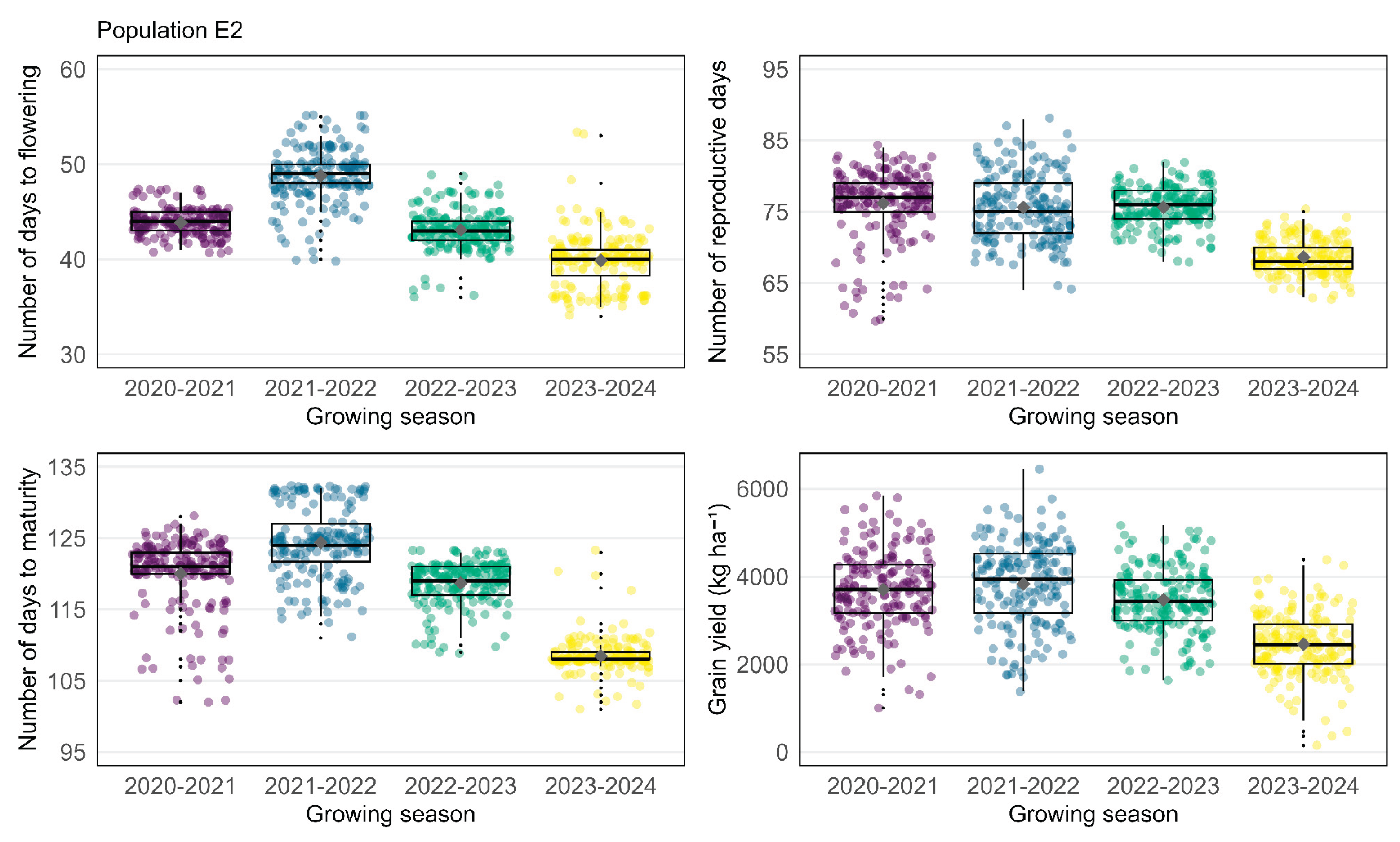
Figure 2.
Distribution of the number of days to flowering, number of reproductive days, number of days to maturity, and grain yield for Population E3 across different growing seasons. Each point represents an experimental plot. The boxes indicate the median, quartiles, and overall range of the data.
Figure 2.
Distribution of the number of days to flowering, number of reproductive days, number of days to maturity, and grain yield for Population E3 across different growing seasons. Each point represents an experimental plot. The boxes indicate the median, quartiles, and overall range of the data.
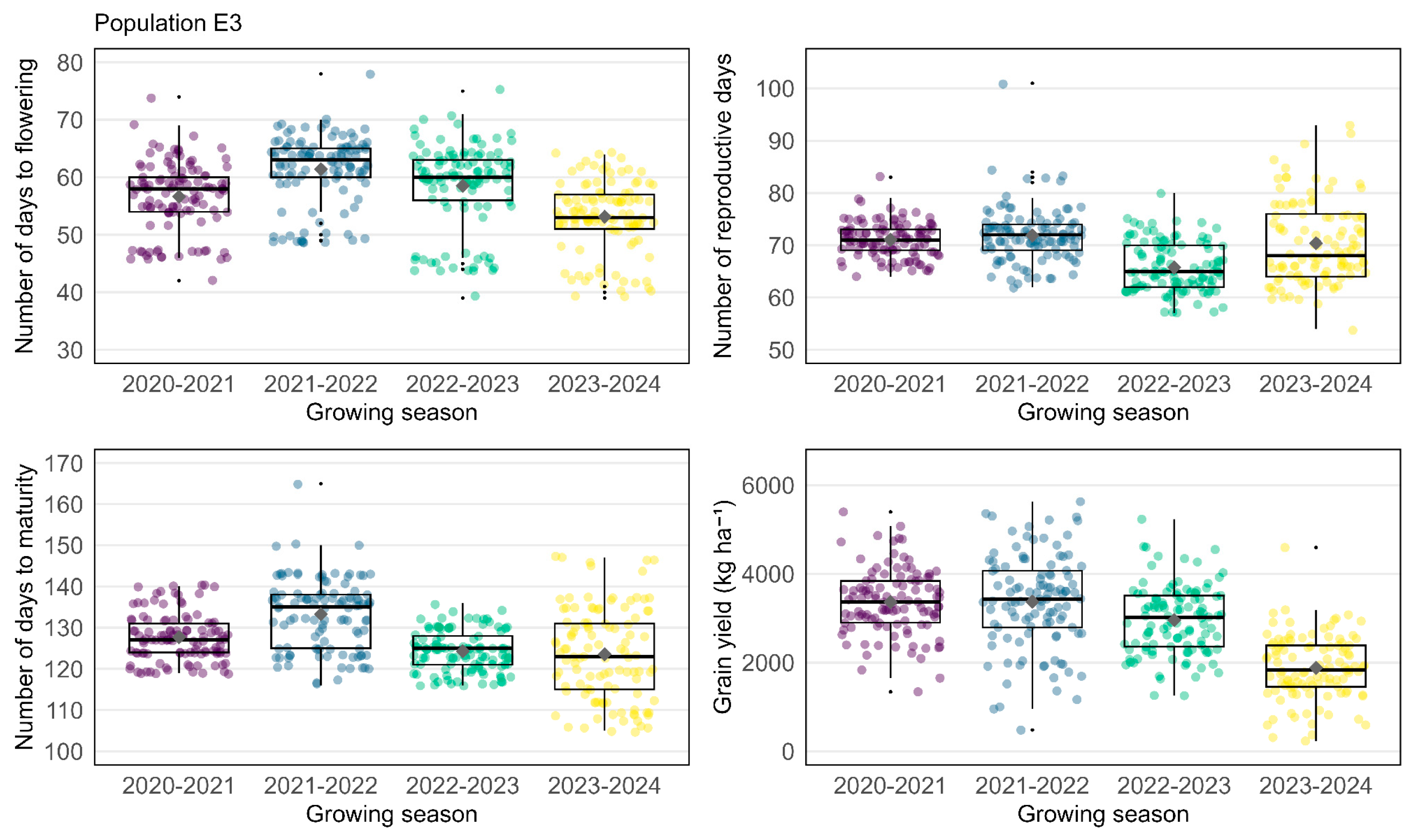
Figure 3.
Two-dimensional dispersion of the BLUPs for number of days to maturity (NDM) and grain yield (GY) of Population E2. The quadrants indicate different performance profiles relative to the population mean: Q1 (highly productive and early), Q2 (low productivity and early), Q3 (highly productive and late), and Q4 (low productivity and late).
Figure 3.
Two-dimensional dispersion of the BLUPs for number of days to maturity (NDM) and grain yield (GY) of Population E2. The quadrants indicate different performance profiles relative to the population mean: Q1 (highly productive and early), Q2 (low productivity and early), Q3 (highly productive and late), and Q4 (low productivity and late).
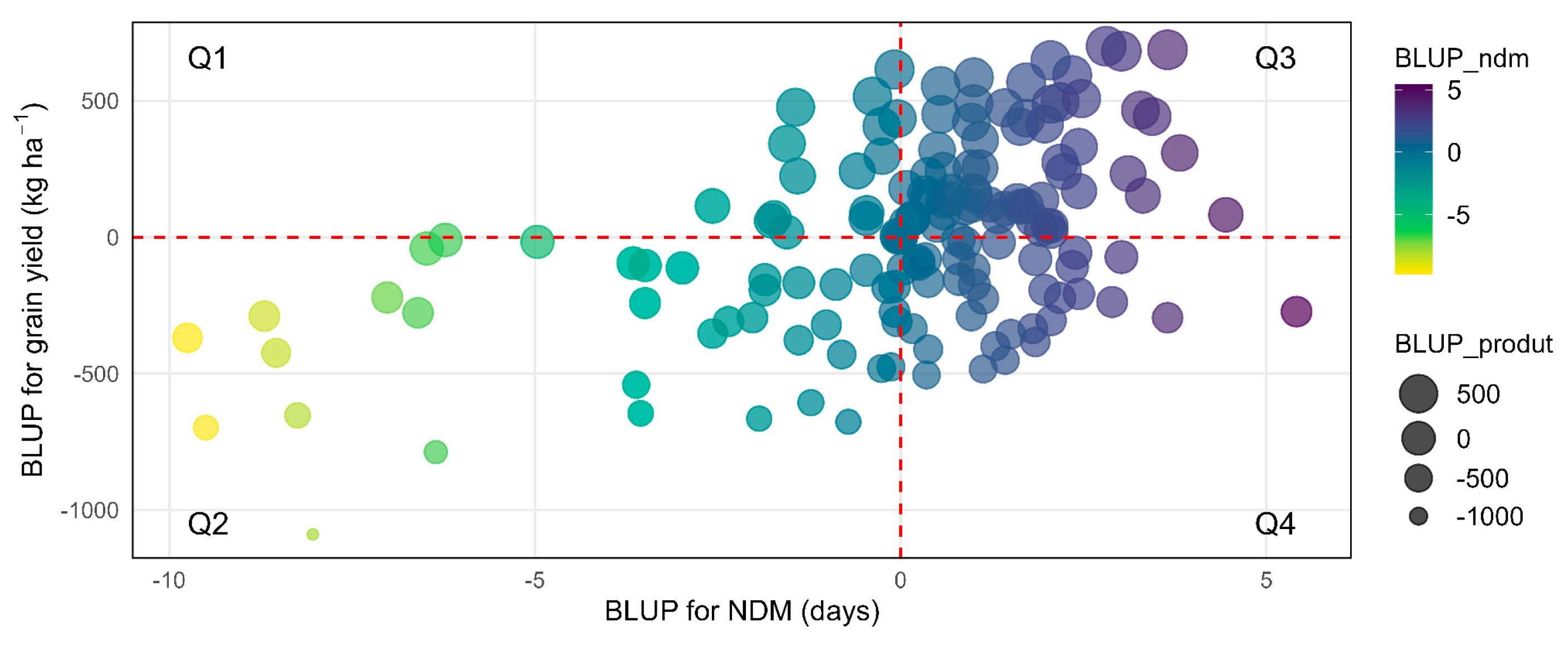
Figure 4.
Two-dimensional dispersion of the BLUPs for number of days to maturity (NDM) and grain yield (GY) of Population E3. The quadrants indicate different performance profiles relative to the population mean: Q1 (highly productive and early), Q2 (low productivity and early), Q3 (highly productive and late), and Q4 (low productivity and late).
Figure 4.
Two-dimensional dispersion of the BLUPs for number of days to maturity (NDM) and grain yield (GY) of Population E3. The quadrants indicate different performance profiles relative to the population mean: Q1 (highly productive and early), Q2 (low productivity and early), Q3 (highly productive and late), and Q4 (low productivity and late).
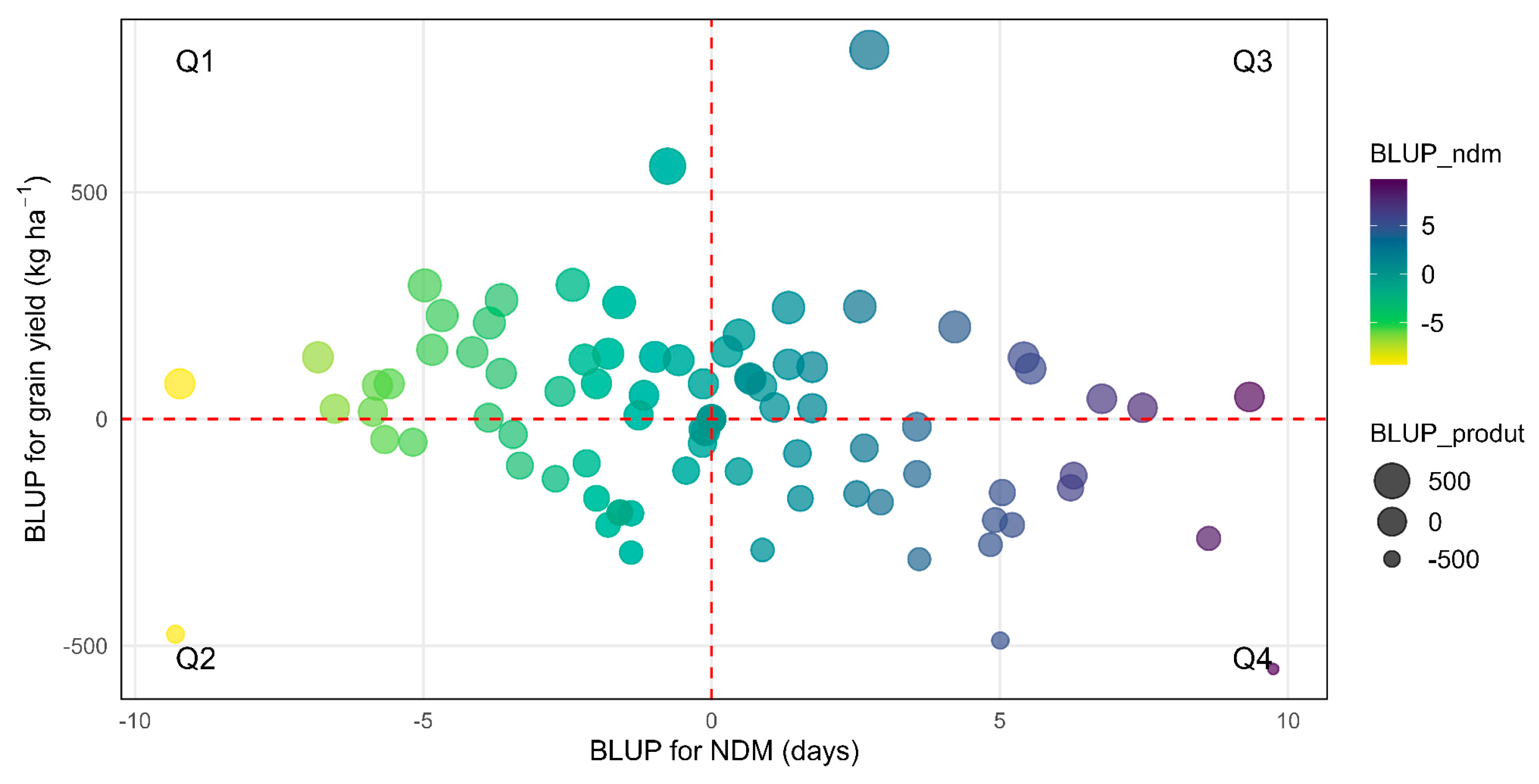
Figure 5.
Marginal predictions of NDF, NRD, and NDM obtained from mixed models adjusted with accumulated precipitation and mean temperature as fixed covariates for Population E2. The blue lines represent the values adjusted according to the covariates, with shading indicating the confidence interval. Jaboticabal, SP.
Figure 5.
Marginal predictions of NDF, NRD, and NDM obtained from mixed models adjusted with accumulated precipitation and mean temperature as fixed covariates for Population E2. The blue lines represent the values adjusted according to the covariates, with shading indicating the confidence interval. Jaboticabal, SP.
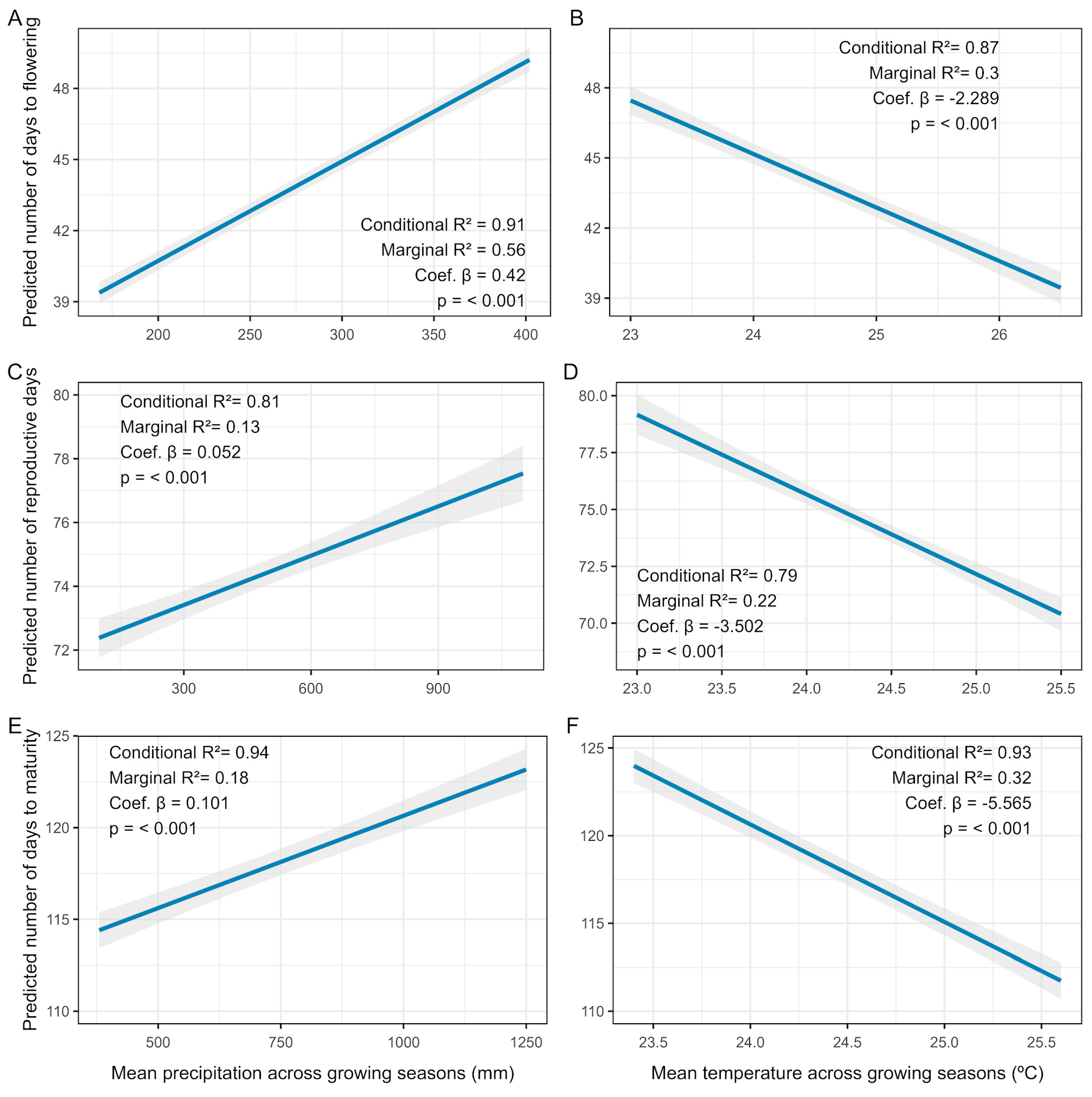
Figure 6.
Marginal predictions of NDF, NRD, and NDM obtained from mixed models adjusted with accumulated precipitation and mean temperature as fixed covariates for Population E3. The blue lines represent the values adjusted according to the covariates, with shading indicating the confidence interval. Jaboticabal, SP.
Figure 6.
Marginal predictions of NDF, NRD, and NDM obtained from mixed models adjusted with accumulated precipitation and mean temperature as fixed covariates for Population E3. The blue lines represent the values adjusted according to the covariates, with shading indicating the confidence interval. Jaboticabal, SP.
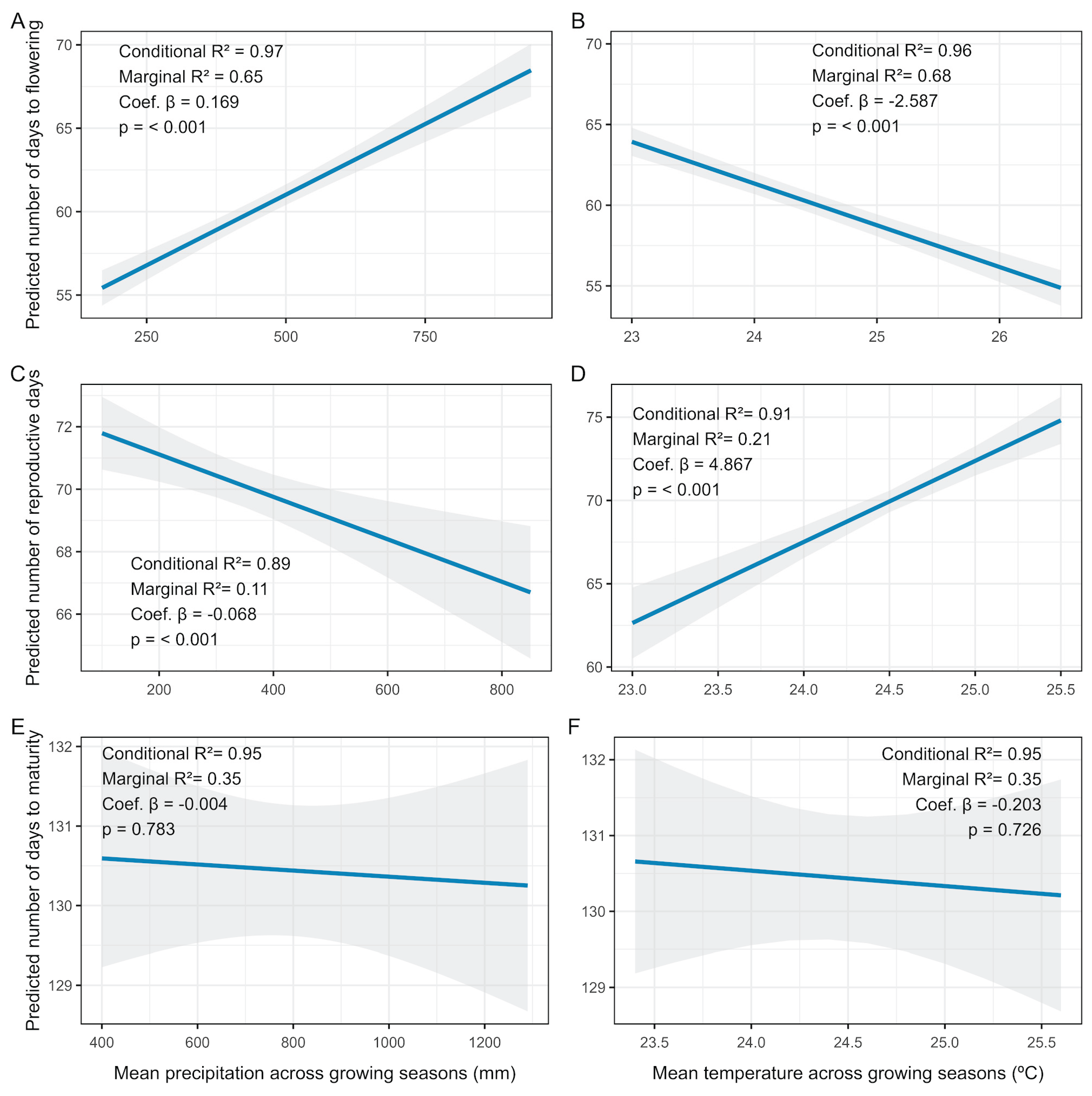
Table 1.
Coefficients of determination (R²) and Type III Wald test results for fixed effects in mixed models fitted for NDF, NRD, NDM, and GY in two soybean populations. Jaboticabal, SP.
Table 1.
Coefficients of determination (R²) and Type III Wald test results for fixed effects in mixed models fitted for NDF, NRD, NDM, and GY in two soybean populations. Jaboticabal, SP.
| Population | Trait | Model R² | Fixed R² | Random R² | Fixed effect | χ² | p-value |
| E2 | NDF | 0.86 | 0.65 | 0.22 | Growing season | 366.26 | <0.001*** |
| Check | 0.27 | 0.97 ns | |||||
| NRD | 0.82 | 0.43 | 0.39 | Growing season | 127.39 | <0.001*** | |
| Check | 2.98 | 0.40 ns | |||||
| NDM | 0.93 | 0.25 | 0.69 | Growing season | 453.93 | <0.001*** | |
| Check | 1.68 | 0.64 ns | |||||
| GY | 0.57 | 0.24 | 0.32 | Growing season | 117.52 | <0.001*** | |
| Check | 1.95 | 0.58 ns | |||||
| E3 | NDF | 0.96 | 0.76 | 0.20 | Growing season | 269.30 | <0.001*** |
| Check | 37.49 | <0.001*** | |||||
| NRD | 0.89 | 0.21 | 0.68 | Growing season | 130.14 | <0.001*** | |
| Check | 2.50 | 0.47 ns | |||||
| NDM | 0.96 | 0.40 | 0.56 | Growing season | 149.40 | <0.001*** | |
| Check | 17.30 | <0.001*** | |||||
| GY | 0.54 | 0.18 | 0.36 | Growing season | 111.68 | <0.001*** | |
| Check | 0.84 | 0.84 ns |
χ²: Chi-square; p-value: significance of fixed effects in each experiment; Check: check genotype. Significance codes: *** p ≤ 0.001; ** p ≤ 0.01; * p ≤ 0.05; p ≤ 0.1; ns: not significant (p > 0.1).
Table 2.
Variance components and genetic parameters for NDF, NRD, NDM, and GY in two soybean populations. Jaboticabal, SP.
Table 2.
Variance components and genetic parameters for NDF, NRD, NDM, and GY in two soybean populations. Jaboticabal, SP.
| Parameter | Population E2 | Population E3 | ||||||
| NDF | NRD | NDM | GY | NDF | NRD | NDM | GY | |
| Variance components | ||||||||
| 2.65 | 4.80 | 9.41 | 192826.96 | 10.21 | 15.84 | 21.23 | 108691.44 | |
| 0.95 | 4.54 | 3.78 | 35436.18 | 2.27 | 9.75 | 14.95 | 68051.73 | |
| 0.44 | 1.36 | 1.35 | 35216.48 | 0.45 | 0.42 | 1.10 | 40124.40 | |
| 2.28 | 4.49 | 3.36 | 433279.93 | 2.11 | 3.80 | 3.18 | 512606.14 | |
| Genetic values | ||||||||
| 0.77 | 0.68 | 0.84 | 0.62 | 0.90 | 0.66 | 0.82 | 0.43 | |
| 0.88 | 0.82 | 0.92 | 0.79 | 0.95 | 0.82 | 0.91 | 0.65 | |
| 3.42 | 2.91 | 1.56 | 18.52 | 2.77 | 2.82 | 1.47 | 24.23 | |
| 3.69 | 3.00 | 2.62 | 12.36 | 6.10 | 4.52 | 3.79 | 11.16 | |
| 1.08 | 1.03 | 1.67 | 0.67 | 2.20 | 1.60 | 2.58 | 0.46 | |
| Mean | 44.12 | 72.89 | 117.01 | 3553.15 | 52.38 | 69.06 | 121.43 | 2953.71 |
Disclaimer/Publisher’s Note: The statements, opinions and data contained in all publications are solely those of the individual author(s) and contributor(s) and not of MDPI and/or the editor(s). MDPI and/or the editor(s) disclaim responsibility for any injury to people or property resulting from any ideas, methods, instructions or products referred to in the content. |
© 2026 by the authors. Licensee MDPI, Basel, Switzerland. This article is an open access article distributed under the terms and conditions of the Creative Commons Attribution (CC BY) license.
Copyright: This open access article is published under a Creative Commons CC BY 4.0 license, which permit the free download, distribution, and reuse, provided that the author and preprint are cited in any reuse.


