

Submitted:
15 July 2026
Posted:
17 July 2026
You are already at the latest version
Abstract
This paper presents a real-time browser-based platform for thermal‑hydraulic characteri-zation of a compact laboratory heat exchanger, implemented within the PolyVR re-search‑grade virtual reality engine. Experimental measurements—including temperature, flow rate, pressure, and electrical quantities—are retrieved from a cloud database at 1 Hz and processed through a browser‑native computational framework that performs contin-uous thermophysical modeling, hydraulic analysis, and energy‑balance evaluation. The system computes heat‑transfer rate, overall heat‑transfer coefficient, Reynolds, Prandtl, Nusselt, and Grashof numbers, pump performance, heater efficiency, and cumulative thermal energy. PolyVR serves as the runtime environment for the digital twin, providing modular integration of browser‑based computation with immersive 3D visualization. The platform supports animated flow diagrams, valve‑state indicators, thermal‑field moni-toring, and interactive manipulation of system components. Its scalable architecture ena-bles deployment across desktops, head‑mounted displays, and CAVE environments, with remote access facilitated through ngrok tunneling. Experimental validation using steady‑state and dynamic datasets demonstrates that the PolyVR‑enabled browser com-putation reproduces laboratory‑grade thermal‑hydraulic analysis with high fidelity, ena-bling accessible remote experimentation, immersive visualization of invisible thermal processes, and VR‑based digital‑twin interaction.
Keywords:
heat exchanger
; thermal hydraulic analysis
; browser-based computation
; cloud database
; real-time visualization
; energy balance
1. Introduction
Real-time thermal-hydraulic characterization plays a fundamental role in the design, optimization and operation of modern energy systems, thermal process equipment and engineering laboratories. Experimental investigation of heat exchangers requires continuous acquisition and analysis of temperature, flow rate, pressure and electrical measurements to evaluate heat-transfer performance, hydraulic behavior and energy efficiency. Conventional laboratory data-acquisition (DAQ) systems generally rely on proprietary software, local processing and dedicated hardware interfaces, limiting system accessibility, scalability, interoperability and remote experimentation [1,2]. The rapid development of cloud computing, Internet of Things (IoT) [12] technologies and browser-based scientific computing has significantly expanded the capabilities of modern engineering platforms. Cloud-connected sensor networks enable reliable real-time transmission of experimental measurements, while advances in web technologies such as WebAssembly permit computationally intensive numerical algorithms to execute directly within web browsers with performance approaching native desktop applications [3,4,5,6]. These developments are facilitated distributed engineering workflows, remote experimentation and collaborative analysis without requiring specialized software installation. Recent research has also demonstrated the growing importance of IoT-enabled laboratory infrastructures for thermal systems. Cloud-based monitoring architectures have been successfully employed for continuous acquisition of temperature, pressure, flow and electrical measurements, supporting automated diagnostics, performance assessment and predictive maintenance of thermal equipment [7,8,9]. At the same time, digital twin methodologies have emerged as an effective framework for integrating experimental measurements with computational models, enabling real-time system monitoring, performance prediction and operation optimization [10,11,13]. Despite this advances, existing browser-based engineering platforms primarily focus on simulation and design rather than real0time experimental characterization. Likewise, many IoT-based laboratory systems provide only measurement acquisition and visualization, while the associated thermal-hydraulic calculations are performed offline using desktop engineering software or post-processing tools. Consequently, relatively few systems integrate cloud-balance calculations and interactive visualization into a unified platform capable of supporting both engineering research and laboratory education [7,8,9,10,11]. This paper addresses this gap by presenting a real-time browser-based platform for thermal hydraulic characterization of a compact water-to-water laboratory heat exchanger. Experimental measurements are continuously retrieved from a cloud database at a sampling frequency of 1 Hz, while all thermophysical calculations are executed directly withing the browser. The computational framework determines the instantaneous heat-transfer coefficient, Reynolds, Prandtl, Nusselt and Grashof numbers, pump hydraulic performance and efficiency, heater performance and cumulative thermal energy. In addition, the platform integrated animated process-flow visualization, valve-state monitoring and thermal imaging to provide a comprehensive representation of the experimental system in real-time. The main contributions of this work are the development of (i) a cloud-connected DAQ architecture for real-time thermal-hydraulic experimentation, (ii) a browser-native computational engine for thermophysical and hydraulic analysis, (iii) an integrated visualization environment for interactive laboratory monitoring and (iv) the experimental validation of the proposed platform using steady-state and transient operating conditions. The proposed architecture provides a scalable foundation for browser-based remote laboratories, digital twin applications and engineering education in thermal-fluid systems. The scientific novelty of this work lies in the real-time integration of cloud-based measurement acquisition, browser-native thermal-hydraulic computation and interactive visualization into a unified platform. Unlike existing IoT laboratory systems that provide only measurement streaming or offline analysis, the proposed architecture performs full thermophysical modeling, hydraulic evaluation and EN 442 compliant energy balance directly in the browser, enabling remote experimentation and digital twin operation. In addition to the computational and IoT aspects, immersive virtual reality (VR) provides a powerful medium for visualizing and interacting with thermal-hydraulic systems. Many thermal processes—such as internal flow structures, temperature gradients, and transient energy transport—are invisible in physical laboratories and difficult for students to conceptualize. By embedding the browser-native physics engine inside PolyVR, the proposed platform enables real-time digital-twin visualization, interactive manipulation of valves and flow paths, and immersive observation of system behavior in CAVE and HMD environments. This integration transforms the heat-exchanger experiment from a conventional measurement task into an interactive VR laboratory, supporting remote experimentation, engineering education, and physically accurate digital-twin interaction.
2. Materials and Methods
The experimental system is shown on Figure 1 and it is consisting of a closed-loop water circuit incorporating a compact laboratory heat exchanger (HE-001), an electrical heater block (B-001), a circulation pump (P-001), an expansion vessel (EV-001) and eight controllable valves (CV-001-CV-008). Seven DS18B20 temperature sensors (T1-T7) measure inlet/outlet, surface and ambient temperature. A Hall-effect flow meter (FM-001) provides volumetric flow rate, while pressure sensors (M-001, M-002) measure pump head [25]. Electrical quantities (voltage, current, power, cumulative energy) are acquired from the heater and pump modules. Table 1. shows the experimental setup connection schemes which are supported, each defining a unique inlet/outlet mapping and valve configuration.
Real-time measurement acquisition is performed using a Firebase Realtime Database. Sensor modules publish temperature, flow, pressure and electrical data at 1 Hz, enabling remote experimentation and synchronized IoT acquisition. The platform retrieves each measurement frame asynchronously, containing:
- T1-T7 temperatures;
- Flow meter raw pulses, filtered L/min, volumetric flow (m3/s);
- Pressure readings (kPa);
- Heater and pump electrical quantities;
- Calibration metadata;
- Valve states;
Flow meter tolerance is evaluated against nominal values (0.03; 0.08 and 0.12 m3/h) using ±5% acceptance band. The specifications of all sensing elements used in the experimental platform are summarized in Table 2. This table provides the measurement ranges, resolutions, sampling rates and physical location of each sensor, ensuring full transparency of the data-acquisition fidelity and supporting reproducibility of the experimental results.
The entire platform is implemented in PolyVR [14,15], research – grade virtual reality 3D engine developed at the Institute for Information Management in Engineering (IMI), Karlsruhe Institute of Technology (KIT) since 2009. PolyVR provides several capabilities essential for this work, such as:
- Modular architecture – enables rapid extension with new computational modules and visualization components;
- Open-source foundation – built on OpenSG and OpenGL, providing high-performance scene-graph backbone with clustering and threading;
- Scalable deployment – supports cave automatic virtual environments (CAVE) [16], visualization clusters, desktops, head mounted devices (HMD) and 3D displays;
- Flexible device integration – through VRPN, ARTTMDTrack and HTTP sockets, PolyVR interfaces with tracking systems, mobile devices and external simulations;
- Rich data import – supports glTF, COLLADA, VRML, STL, OBJ, IFC, STEP, E57, SVG, DWG, DXF and more;
Within this, PolyVR functions as a runtime host for browser-native computational engine, a visualization framework for animated hydraulic schematics, valve indicators, flow-path overlays, thermal camera streaming and a local server enabling offline execution on laboratory workstations. When tunneled through ngrok [17], PolyVR additionally serves as a public deployment host, allowing remote users to observe or interact with live experiments. To evaluate cross-platform robustness, the system was tested on a PICO4 HMD and on our custom-built MAGURA CAVE environment, confirming stable rendering performance and full compatibility with immersive visualization setups. PolyVR’s research pedigree and extensible design therefore provide a credible foundation for developing a browser-native digital twin of the thermal-hydraulic system.
Figure 2 illustrates the complete visualization pipeline, beginning with the physical laboratory system, followed by its PolyVR virtual model, deployment in the MAGURA CAVE immersive environment, and direct user interaction. All thermal-hydraulic calculations are executed directly within the browser using JavaScript and WebAssembly-compatible routines, enabling real-time browser computation without external numerical libraries or server-side processing. Each incoming sensor frame (1 Hz) triggers a full update of thermophysical properties, hydraulic quantities, thermal performance metrics and dimensionless numbers, ensuring synchronized visualization and analysis across the PolyVR environment. All internal calculations are performed strictly in SI units (K, Pa, m3/s, kg/s, W, J), guaranteeing physical consistency and compliance with EN 442 requirements [18,19]. For user clarity, the platform simultaneously displays both SI and “user-friendly” units, such as temperature in K and °C, flow rate in m3/s, L/s, L/min and mass flow in kg/s, as shown in Figure 3.
Thermophysical properties of water are updated dynamically using empirical correlations selected for their accuracy within the operating range of radiator and heat-exchanger systems (293.15-353.15K). These properties directly influence Reynolds, Prandtl, Grashof and Nusselt numbers and therefore the convective heat-transfer coefficient h. Water density is evaluated using the linearized correlation shown in Equation (1)
Density is computed using a linearized correlation valid for 293.15 – 353.15 K, ensuring correct mass flow and hydraulic calculations. This approximation captures the gradual reduction in density as temperature increases and is used in mass flow, Reynolds number and hydraulic power calculations. The specific heat capacity is computed as shown in Equation (2).
Equation (2) represents a simplified linear approximation of the temperature dependence of water’s specific heat capacity over the considered range. The term 4184.4 is the reference value at 293.15 K, while -0.9 describes its weak temperature dependence. This property directly determines thermal power and enthalpy transport. This parameter is used in all thermal calculations, including heat-output determination, heater efficiency and enthalpy-based mass-flow rate.
Dynamic viscosity is computed using the Vogel correlation [20] as represented in Equation (3), which accurately captures the nonlinear temperature dependence of water in the 293.15-353.15 K range. The empirical constants A, B and C are selected to match the operating conditions of the HeatLab loop, ensuring correct Reynolds number evaluation under real-time browser computation. Thermal expansion coefficient is defined in Equation (4).
In Equation (4) β represents volumetric expansion per unit temperature change. is a reference absolute temperature. This simplified approximation is used only for buoyancy estimation in the Grashof number where detailed tabulated water data is not employed to quantify the buoyancy-driven natural convection. Kinematic viscosity is computed as in Equation (5).
where ν represents momentum diffusivity, μ is dynamic viscosity and is density. This parameter governs the ratio of viscous to inertial forces and is used in Reynolds and Grashof numbers calculations. These thermophysical properties shows in Equations (1)–(5). are continuously updated to ensure consistent prediction of flow regime, convective heat transfer and energy balance. Hydraulic quantities are derived from real-time measurements of volumetric flow rate and pressure. The mass flow rate is calculated as:
Equation (6) converts volumetric flow rate to mass flow rate and is required for heat-output calculations, heater efficiency and advective energy transport. Pump head determination is represented in Equation (7), representing the mechanical energy added to the fluid per unit weight.
Hydraulic power is then computed as in Equation (8), quantifying the useful hydraulic work delivered by the pump and pump efficiency is evaluated as in Equation (9), comparing hydraulic power to electrical input power.
Thermal performance is computed from inlet and outlet temperatures, which depend on the hydraulic connection scheme (Table 1) and the mass flow rate. The instantaneous heat-transfer rate is:
Equation (10) represents the advective thermal energy removed from the radiator by the circulating water. This is primary quantity used in EN 442 conformity assessment. The log-mean temperature difference (LMTD) is evaluated as:
Equation (11) accounts for the non-uniform temperature difference between the radiator and the surrounding air. The overall heat-transfer coefficient is then obtained from Equation (12), characterizing the radiator’s ability to transfer heat to the room.
Dimensionless numbers quantify flow regime and convective behavior. The Reynolds number is computed as in Equation (13) and determines whether the internal flow is laminar, transitional or turbulent. The Prandtl number is given by Equation (14), comparing momentum diffusivity to thermal diffusivity and the Grashof number is evaluated as in Equation (15), quantifying buoyancy-driven natural convection on the air side of the radiator.
The Nusselt number is evaluated using the classical correlation for internal forced convection as represented in Equation (16).
Laminar and turbulent convection inside the radiator channels is evaluated using the Sieder-Tate (Equation (17)) and Dittus-Boelter correlations [21,22], consistent with EN 442 methodology. Because radiator channels are short, narrow and operate with small wall-bulk temperature differences (<5K), viscosity-corrected formulations provide negligible benefit. The browser engine therefore applies the EN 442 endorsed correlations to ensure stable, physically accurate real-time computations. The convective heat-transfer coefficient is then obtained from Equation (18).
Radiator is modeled as a single thermal mass with uniform temperature. This lumped-capacity assumption is valid only when internal conduction within the radiator metal is much faster than external convection. This condition is quantified using the Biot number, which is represented in Equation (19).
The radiator is modeled as a lumped thermal mass because its Biot number is very small (Bi ≪0.1). Typical steel conductivity (≈45 W/m.K), measured convection coefficient (5-12 W/m2.K) and wall thickness (0.5-1.5 mm) confirm negligible internal temperature gradients. This assumption is fully consistent with the standard and enables a stable first-order transient model suitable for real-time browser computation. The thermal power balance describes how energy flows through the heater-radiator-water system and provides a physically consistent framework for interpreting both steady-state and transient measurements. In the HeatLab platform, this balance is computed in real-time using SI-unit calculations, ensuring compatibility with requirements and enabling direct comparison between measured and modeled quantities. At the core of the system is the electrical power input supplied to the heater block. The platform records the cumulative electrical energy and computes the instantaneous electrical power as represented in Equation (20).
Equation (20) represents the total rate at which electrical energy is delivered to the heater. This power is the primary energy source driving the thermal processes in the system. A portion of this electrical input is converted into thermal energy transferred to the circulating water. The heater block raises the water temperature from to and the corresponding thermal power is:
In Equation (21) is the mass flow rate and is the instantaneous specific heat capacity of water. This term quantifies the useful thermal energy imparted to the water loop. The ratio of this thermal output to the electrical input defines the heater’s thermal efficiency which is represented in Equation (22).
Once heated, the water transport energy to the radiator, where it releases heat to the surrounding air. The radiator heat output is determined from the advective energy removed by the water.
Equation (23) represents the actual emitted heat under the current operating conditions and is the principal metric used for EN 442 conformity assessment. Because it is derived directly from measured temperatures and flow rate, it provides a robust and physically grounded indicator of radiator performance. Heat transfer from the radiator to the room occurs through both convection and thermal radiation. Convective heat loss is modeled as:
In Equation (24). is the convective heat-transfer coefficient obtained from dimensionless correlations, is the radiator surface area and is the mean radiator temperature. Radiative heat loss is described by Equation (25) with denoting surface emissivity and the Stefan-Boltzmann constant.
Under steady-state conditions, these two mechanisms are combined into an effective overall heat-transfer coefficient U.
Equation (26) simplifies analysis while preserving physical accuracy. Although small compared to thermal power, the hydraulic subsystem also contributes mechanical energy to the water. The hydraulic power delivered by the pump is represented in Equation (27).
In Equation (27) is the pump head. The term is included for completeness, particularly in dynamic experiments where pump speed changes influence the thermal response. The instantaneous energy balance of the system is expressed in Equation (28) which indicates whether the radiator is accumulating energy (positive ) or releasing more energy than it receives (negative ).
During warm-up phases, the radiator’s thermal inertia causes , while in cool-down phases the opposite occurs. Cumulative electrical and thermal energies are obtained by integrating the instantaneous powers expressed in Equations (29) and (30) and the cumulative energy balance in Equation (31).
This cumulative balance is used extensively in validation experiments to detect sensor drift, calibration errors, or inconsistences between measured and modeled behavior. To comply with the standard, the measured heat output must be normalized to standardized temperature differences. The arithmetic mean temperature difference is expressed in Equation (32) and the corrected heat output is expressed in Equation (33)
In Equation (33) is the measured heat output and are regression parameters defined in Annex D of EN 442. Standardized heat outputs at 30 K and 50 K are then expressed in Equations (34) and (35).
Heat outputs represented in Equations (34) and (35) are then allowing direct comparison with manufacturer data and regulatory specifications. The thermal power balance forms the analytical foundations for all experimental activities carried out in the HeatLab facility. The complete experimental program is structured into three series-S, D and V-each of which uses the power balance formulation in a different way to characterize radiator behavior, validate measurements and support mathematical modeling. The S-series (steady-state) (S1-S14) experiments apply the thermal power balance under stationary operating conditions. In these tests, the system is allowed to reach thermal equilibrium, enabling direct evaluation of the radiator’s heat-transfer performance trough quantities such as overall heat-transfer coefficient U, the convective coefficient h and the dimensionless numbers Re,Pr,Gr and Nu. Because the system is in steady state, the instantaneous energy balance closes tightly, allowing verification of EN 442 conformity, including the determination of standardized heat outputs and . These experiments establish reference operating points and quantify how hydraulic configuration and flow regime influence radiator performance. The D-series (dynamic) (D1-D4) experiments use the full transient form of the thermal power balance to investigate the radiator’s response to controlled disturbances. Step changes in heater power, pump speed transitions and control valve restrictions introduce rapid variations in flow rate, temperature difference and convective regime. The resulting transient behavior reveals the radiator’s thermal inertia, time constant, overshoot/undershoot characteristics and the dynamic coupling between hydraulic and thermal subsystems. These experiments are essential for validating the mathematical model and supporting digital-twin development, where accurate prediction if transient behavior is required. The V-series (validation) (V1-V4) verify the accuracy and consistency of all measurement channels, including temperature sensors, flow meter, pressure transducers, pump hydraulic performance and heater electrical output. Each subsystem is validated individually and collectively to ensure that deviations between the measured and modeled thermal power – whether instantaneous or cumulative – serve as reliable indicators of calibration drift, sensor bias or hydraulic anomalies. These validation procedures ensure traceability and confidence in all subsequent steady-state and dynamic analyses. Underlying all three experimental series is the HeatLab Protocol, a comprehensive methodology developed specifically for this laboratory system. The protocol is fully aligned with the principles of EN 442 but extends them to accommodate the unique characteristics of the HeatLab radiator, heater block, hydraulic network and sensor architecture. EN 442 provides the standardized framework for radiator testing, including definitions of temperature differences, correction factors, regression parameters and steady-state requirements. The HeatLab Protocol operationalizes these principles by:
- Defining structured experimental matrices for hydraulic configurations, pump speeds and heater power levels;
- Specifying measurement procedures, calibration workflows and commissioning steps;
- Integrating real-time thermophysical property updates and browser-native computation;
- Extending EN 442 steady-state methodology to dynamic (D-series) and validation (V-series) contexts;
- Embedding the mathematical modeling directly into the experimental workflow;
In this way, the HeatLab Protocol not only endorses the standard but also expands it to create a unified, reproducible and physically rigorous methodology tailored to the specific laboratory system. It ensures that every measured quantity, delivered parameter and modeled response is grounded in the standardized radiator-testing practice while remaining flexible enough to support advanced research, transient modeling and digital twin development. Figure 4 presents the PolyVR 3D digital-twin model of the HeatLab radiator test bench, showing fully virtualized representation of the hydronic heating loop used in the experimental protocol. The model mirrors the physical laboratory system in real-time, displaying live thermal-hydraulic measurements including water temperatures, pressure levels and volumetric flow rate at key locations throughout the circuit. The virtual environment reproduces all major components of the HeatLab setup – the heater module, the circulation pump, the radiator, the piping network and the sensor array. Temperature readings at the heater inlet/outlet, radiator inlet/outlet and return line are visualized directly on the 3D model, enabling intuitive interpretation of heat distribution and flow behavior. Pressure sensors and flow meter outputs are similarly integrated, providing a complete overview of hydraulic performance. In the upper right corner, the model includes a real-time telemetry graph that plots temperature evolution for multiple system nodes, flow rate and pressure. This visualization allows users to observe transient behavior, thermal stabilization and dynamic responses during S-, D- and V-series experiments. The graph is synchronized with the physical test bench, ensuring that the digital twin reflects the actual system state with high fidelity. The PolyVR model is fully aligned with the HeatLab Protocol, which extends the EN 442 methodology into a modern, simulation-ready framework. By combining real-time data acquisition with interactive 3D visualization, the digital twin supports advanced analysis, scenario testing and educational demonstrations. It also serves as the computational foundation for future control-strategy development, transient modeling and digital-twin based optimization of hydronic heating systems.
Temperature readings at the heater inlet/outlet, radiator inlet/outlet and return line are visualized directly on the 3D model, enabling intuitive interpretation of heat distribution and flow behavior. Pressure sensors and flow meter outputs are similarly integrated, providing a complete overview of hydraulic performance. In the upper right corner, the model includes a real-time telemetry graph that plots temperature evolution for multiple system nodes, flow rate and pressure. This visualization allows users to observe transient behavior, thermal stabilization and dynamic responses during S-, D- and V-series experiments. The graph is synchronized with the physical test bench, ensuring that the digital twin reflects the actual system state with high fidelity. The PolyVR model is fully aligned with the HeatLab Protocol, which extends the EN 442 methodology into a modern, simulation-ready framework. By combining real-time data acquisition with interactive 3D visualization, the digital twin supports advanced analysis, scenario testing and educational demonstrations. It also serves as the computational foundation for future control-strategy development, transient modeling and digital-twin based optimization of hydronic heating systems. The extended thermal power balance provides a detailed decomposition of heat flow through the heater-radiator-water loop and enables a physically transparent interpretation of subsystem behavior. In the HeatLab platform, this balance is computed in real-time. The first component of the balance is the radiator useful thermal output, defined in Equation (36).
Equation (36) represents the actual heat emitted by the radiator to the surround air. Because directly reflects convective and radiative transfer from the radiator surface, is the primary EN 442 performance metric and forms the basis for standardized heat output evaluation. The second component, the cold line losses is expressed in Equation (37).
Equation (37) is quantifying the heat dissipated along the return line between the radiator outlet and the heater inlet. This term is sensitive to pipe insulation quality, ambient temperature and hydraulic layout and therefore provides insight into distribution line efficiency. The third component, the hot line losses is given in Equation (38), representing the heat lost in the supply line from the heater outlet to the radiator inlet. These losses capture conduction and convection effects along the upstream piping and are influenced by heater placement, pipe routing and thermal insulation.
The fourth component of the balance is the heater block delivered thermal power, defined in Equation (39).
Equation (39) describes the enthalpy increase of the water as it passes through the heater block (B-001). This term represents the actual thermal output of the heater and is used to evaluate heater performance and electrical-to-thermal conversion efficiency. The fifth component, the heater block internal losses, is expressed in Equation (40), quantifying the difference between electrical input power and useful thermal output.
Internal losses include conduction through the heater casing, convective losses to ambient air, imperfect insulation, electrical-measurement noise and transient storage effects. This term is essential for diagnosing heater efficiency and verifying the accuracy of electrical-to-thermal conversion. The extended thermal power balance implemented in the HeatLab platform is further illustrated by the real0time stacked power-balance chart shown in Figure 5. This visualization captures the simultaneous evolution of all five-thermal-power components during an active experiment, providing a dynamic representation of how heat is generated, transported, emitted and lost throughout the hydraulic loop.
The chart shown on Figure 5 displays the radiator useful thermal output , the cold line losses , the hot line losses , the heater block delivered thermal power and the heater block internal losses , each plotted both as absolute power and as a percentage of the electrical input . The stacked regions reveal the cumulative contribution of each subsystem, while the overlaid percentage curves highlight how the relative shares of supply line losses, return line losses, radiator emission and heater performance evolve over time. This real-time decomposition enables direct observation of transient phenomena such as flow rate changes, heater power transitions, thermal stabilization and it provides immediate diagnostic insight into insulation quality, hydraulic configuration and heater efficiency. Unlike conventional laboratory DAQ systems – which typically compute only the radiator heat output – the HeatLab platform resolves the entire hydraulic loop into physically meaningful thermal segments, allowing verification of EN 442 regression inputs, identification of anomalous loss patterns and confirmation of energy balance closure. The resulting chart therefor serves as a digital-twin grade diagnostic tool, demonstrating the capability of the browser-native computation engine to track and interpret complex thermal-hydraulic interaction with high temporal fidelity.
3. Results
The experimental campaign conducted on the HeatLab platform encompassed all operating modes defined in the protocol, including steady-state characterization (S-series), dynamic transient tests (D-series) and measurement-chain validation (V-series). These experiments were executed according to structured matrices, ensuring systematic coverage of hydraulic layouts, heater power levels, pump speed and flow-regime conditions. The S-series represented in Table 3 established the radiator’s thermal-hydraulic behavior under controlled stationary conditions, enabling evaluation of convection regimes, EN 442 parameters and energy balance closure. The extended hydraulic configurations represented in Table 4 provided additional insight into asymmetric, alternative and intentionally unfavorable flow distributions, revealing their influence on temperature stratification and radiator performance. The D-series experiments represented in Table 5 investigated transient responses to heater power jumps, pump speed transitions and controlled flow restriction, supporting analysis of system inertia, regime transitions and coupled thermo-hydraulic dynamics relevant to digital-twin development. Finally, the V-series validation tests represented at Table 6 confirmed the accuracy and reliability of all sensing elements, including temperature sensors, flow meter, pressure transducers, pump curve and heater electrical output, ensuring traceability and confidence in the subsequent analysis. Together, these experimental groups form a comprehensive dataset that supports both fundamental thermal-hydraulic interpretation and advanced digital-twin modeling.
3.1. Overview of Conducted Experiments
The complete set of experimental configurations is summarized in structured matrices. These matrices specify the hydraulic scheme, heater power level, pump speed and target flow regime for each experiment, forming the basis for interpreting the results presented in the following subsections.
3.2. Steady-State Results (S-Series)
The steady-state experiments (S1-S11) revealed clear distinctions between hydraulic configurations and heater power levels. The reference operating point (S2), corresponding to the top-bottom (diagonal) scheme at 1 kW heater power and a medium number, consistently produced stable flow conditions around 0.08 m3/h (2.22e-5 m3/s) (Figure 6 and Figure 7) and a radiator heat output of approximately 600-700 W.
The Reynolds number (Figure 8) remained in the transitional regime (2500-5000) and the Nusselt number (Figure 11) ranged between 15 and 30, indicating mixed convection behavior typical for compact radiator channels. In addition to forced convection indicators, the Prandtl number (Figure 9) gradually decreased from approximately 6.4 to 3.0 as the water temperature increased, reflecting the expected reduction in dynamic viscosity and confirming the thermophysical consistency of the browser-native property calculations. The Grashof number (Figure 10) rose steadily toward values on the order of 1013, indicating the presence of buoyancy-driven natural convection on the air side of the radiator surface, although these remained secondary compared to the dominant forced-convection regime inside the water channels.
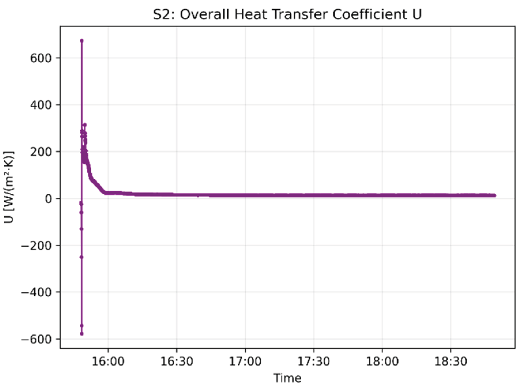
The overall heat-transfer coefficient (Figure 13) exhibited minimal variance (12.2-13.95 W/m2. K), confirming the stability of the radiator’s thermal performance under steady-state conditions (Figure 12).
The EN 442 regression (Figure 14) applied to the S2 dataset produced a correction curve within confidence band, demonstrating that browser-native computation reproduces laboratory-grade analysis. The energy balance closed tightly, with cumulative electrical and thermal energies differing only by the expected thermal inertia of the radiator mass.
Figure 11.
Nusselt number evolution over time.
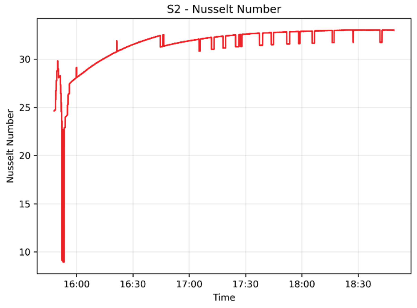
Figure 12.
Electrical vs. thermal power.
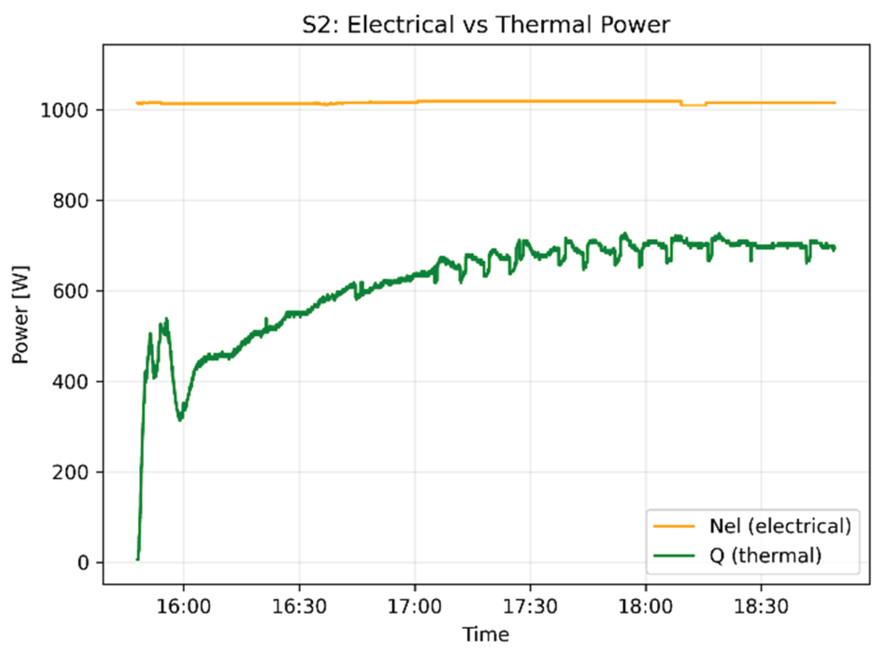
Figure 13.
Overall heat-transfer coefficient U over time.
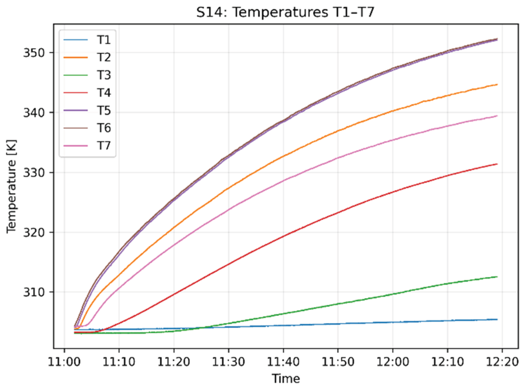
The extended hydraulic configurations (S12-S14) demonstrated the sensitivity of radiator performance to inlet/outlet asymmetry. The uniliteral top-bottom (S12) produced measurable temperature stratification with reduced uniformity across the radiator surface. The bottom-top (diagonal) configuration (S13) showed improved distribution compared to its uniliteral counterpart (S14), confirming that diagonal flow paths enhance convective uniformity. The worst-case distribution (S14) resulted in lower Reynolds numbers, reduced Nusselt numbers and increased line losses, consistent with theoretical expectations for asymmetric flow. These results highlight the importance of hydraulic layout in radiator performance and validate the ability of the HeatLab platform to resolve subtle differences in flow distribution. The temperature evolution for each configuration is shown in Figure 15, Figure 16 and Figure 17.
Figure 14.
EN 442 vs. regression with band.
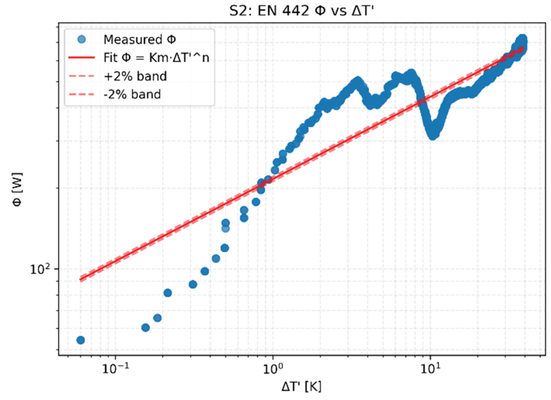
Figure 15.
Temperature evolution at sensors T1-T7 (top-bottom uniliteral).
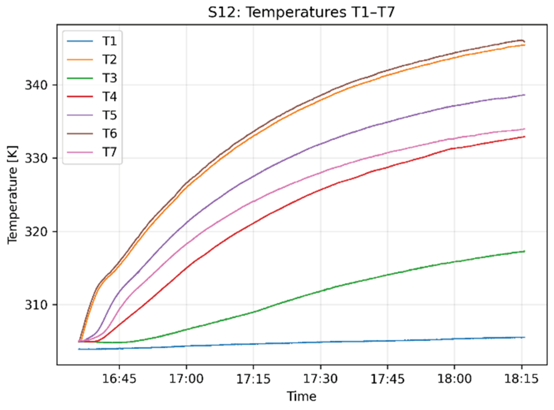
In the uniliteral top-bottom configuration (S12), the temperature curves exhibit clear stratification. As shown in Figure 15, sensors located near the inlet reach significantly higher temperatures than those near the outlet. The spread between the curves remains large throughout the experiment, indicating non-uniform convective distribution inside the radiator. This behavior is characteristic of uniliteral flow paths, where water enters and exists on the same side, reducing the effective sweep of the radiator channels and limiting thermal uniformity.
The bottom-top diagonal configuration (S13) shows marked improvement in temperature uniformity. As illustrated in Figure 16, the temperature curves rise more consistently across all sensors, with reduced separation between inlet and outlet readings. This confirms that diagonal flow paths promote more homogeneous convective coverage, improving heat distribution across the radiator surface. The diagonal configuration therefore serves as a reference for balanced hydraulic behavior and is consistent with EN 442 recommendations for radiator testing. The bottom-top uniliteral configuration (S14) represents the worst-case distribution. Figure 17 shows pronounced temperature divergence. This asymmetry indicates poor internal flow distribution, reduced Reynolds number and diminished convective effectiveness. The resulting temperature gradients are larger than in S12 and S13, confirming that uniliteral bottom-top flow produces the least favorable thermal performance.
Figure 16.
Temperature evolution at sensors T1-T7 (bottom-top diagonal).
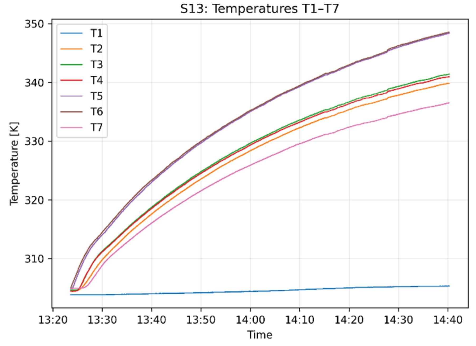
Figure 17.
Temperature evolution at sensors T1-T7 (bottom-top uniliteral).
3.3. Dynamic Response (D-Series)
The dynamic experiments (D1-D4) were designed to investigate the transient thermal-hydraulic behavior of the HeatLab system under controlled disturbances. These tests introduce rapid changes in heater power, pump speed and flow restriction, allowing evaluation of system inertia, convection regime transitions and the coupling between hydraulic and thermal subsystems. The results demonstrate that the browser-native computation engine captures transient phenomena with high temporal fidelity, without numerical oscillations or instability. All dynamic tests use the “top-bottom (diagonal)” hydraulic scheme with a reference flow rate of 2.22e-5 m3/s, as it serves as the reference configuration for transient analysis. For D-series test presented in Table 5 involving heater power changes (D1, D4), the electrical power is changed in a single step from 500 W to 1500 W (and vice versa), with switching time shorter than 5 seconds, i.e., effectively instantaneous relative to the thermal time constant of the system. D4 is combined thermal and hydraulic transition, in which the electrical power of the heater is changed from 500 W to 1500 W within an interval of less than 5 second and the pump speeds are switched according to the given scenario. During the entire experiment, the flow rate is considered practically constant and maintained around 2.22e-5 m3/s, without introducing additional restriction through the valve. After the transition is completed, the system is monitored for 3 – 5 minutes to register the associated thermo-hydraulic response. The transition is carried out in two steps, namely:
- Step #1 (thermo-hydraulic jump) – the electrical power is changed from 500 W to 1500W within the time interval of less than 5 seconds and the pump speed is switched from 1st to 2nd stage (45 W to 67W) when the power reaches 1000 W;
- Step #2 (pure hydraulic jump) – the electric power of the electric heater remains 1500 W and the pump is switched from 67 W to 93 W (from 2nd to 3rd stage). After the pump is switched, the system stands by for 3 – 5 minutes to record the data;
The D1 experiment evaluates the radiator’s thermal inertia by applying a sudden heat power increase from 500 W to 1500 W. The temperature evolution shown in Figure 18. demonstrates the characteristic first-order thermal response of the system. The inlet side sensors react almost immediately to the power step, exhibiting a sharp rise in temperature, while the outlet sensors follow with a measurable delay corresponding to the water’s transport time and the radiator’s internal thermal mass. Sensor T1, located at the ambient reference point, remains nearly constant, confirming stable environmental conditions.
The corresponding electrical and thermal power evolution is presented in Figure 19. The electrical power exhibits an instantaneous jump from 500 W to 1500 W, while the thermal power increases gradually from approximately 350 W to 700 W, reflecting the radiator’s finite thermal inertia and the time required for the water to reach its new steady-state temperature. The smooth rise of thermal power without overshoot confirms the stability of the radiator’s transient response and validates the lumped capacity assumption used in the mathematical model. The D2 experiment investigates hydraulic regime transitions by switching pump speeds in discrete steps (Table 5). The flow rate evolution shown in Figure 20. exhibits two clear stepwise increase corresponding to pump stages 45 W → 67 W → 93 W. Each step produces an immediate rise in volumetric flow rate, demonstrating the responsiveness of the hydraulic subsystem and the accuracy of the flow meter filtering.
The corresponding Reynolds and Nusselt number transitions are shown in Figure 21 and Figure 22. Reynolds number increases from approximately 3000 to nearly 6000, crossing deeper into transitional and early turbulent regime. The Nusselt number follows the same stepwise pattern, rising from ~28 to ~42, confirming the expected increase in convective heat-transfer coefficient with higher flow velocity. These results demonstrate that the HeatLab platform accurately resolves hydraulic disturbances and correctly computes dimensionless quantities in real-time.
The D3 experiment introduces a partial valve restriction to reduce flow rate and force drop in Reynolds number. The temperature evolution shown in Figure 23 reveals immediate rise in radiator outlet temperatures once the valve is partially closed, while inlet temperatures remain comparatively stable. This behavior reflects the reduced convective removal of heat from the radiator when mass flow decreases.
The flow rate response shown in Figure 24 confirms a sharp drop from approximately 2.2e-5 m3/s to 1.4e-5 m3/s, after which the system stabilizes at lower flow level. The inverse relationship between flow rate and temperature difference is clearly visible – as flow decreases, increases due to reduced advective transport. The experiment validates the platform’s ability to capture flow-induced thermal transitions and demonstrates correct computation of Reynolds number reduction under hydraulic restriction as shown in Figure 25.
The D4 experiments is the most complex dynamic scenario, combining both heater power and pump speed transitions. The electrical and thermal evolution shown in Figure 26. illustrates the coupled nature of the disturbance. The electrical power jumps from ~550 W to ~1600 W within seconds, producing an immediate rise in thermal power from ~200 W to ~700 W. After the heater step, thermal power gradually stabilizes near 600 W as the radiator approaches its new operating point. The flow rate response shown in Figure 27. exhibits two distinct hydraulic transitions corresponding to pump stages 45 W → 67 W → 93 W. Each step produces a clear increase in flow rate, rising from ~2.3e-5 m3/s to ~3.0e-5 m3/s. The combined effect of thermal and hydraulic jumps produces a characteristic transient patter - rises sharply during heater step, then decreases as flow increases and convective removal becomes more effective. The smooth stabilization of both thermal and hydraulic quantities confirms that the HeatLab platform accurately models multi-variable transients and that the browser-native computation engine handles coupled disturbances without numerical artifacts. This experiment demonstrates the full dynamic interaction between heater, pump and radiator, validating the extended thermal power balance under non-stationary conditions.
3.4. Validation Results (V-Series)
The V1 validation experiment verifies the accuracy, stability and repeatability of all seven DS18B20 temperature sensors used throughout the HeatLab platform. This procedure is essential because inlet, outlet, surface and ambient temperature form the basis of EN 442 heat output calculations, number evaluation and the thermal power balance. Ensuring that all sensors operate within the required tolerance band is therefore a prerequisite for reliable steady-state and dynamic analysis. The hydronic loop was configured in the endorsed “top-bottom (diagonal)” connection scheme, identical to the reference configuration used in the S-series experiments. The circulation pump maintained a stable reference flow rate of 2.22e-5 m3/s to ensure uniform mixing and eliminate thermal stratification. The heater remained switched off to create an isothermal environment, allowing direct comparison between sensor readings and the thermal camera reference. Thermal reference measurements were obtained using a Testo 860i infrared camera and processed in IRSoft [23]. Data acquisition began only after the loop reached a stable, well-mixed thermal state. For each sensor, deviations were computed as represented in Equation (41). and evaluated against the acceptance criterion of , as specified in Table 6.
Figure 27.
Flow rate evolution over time.
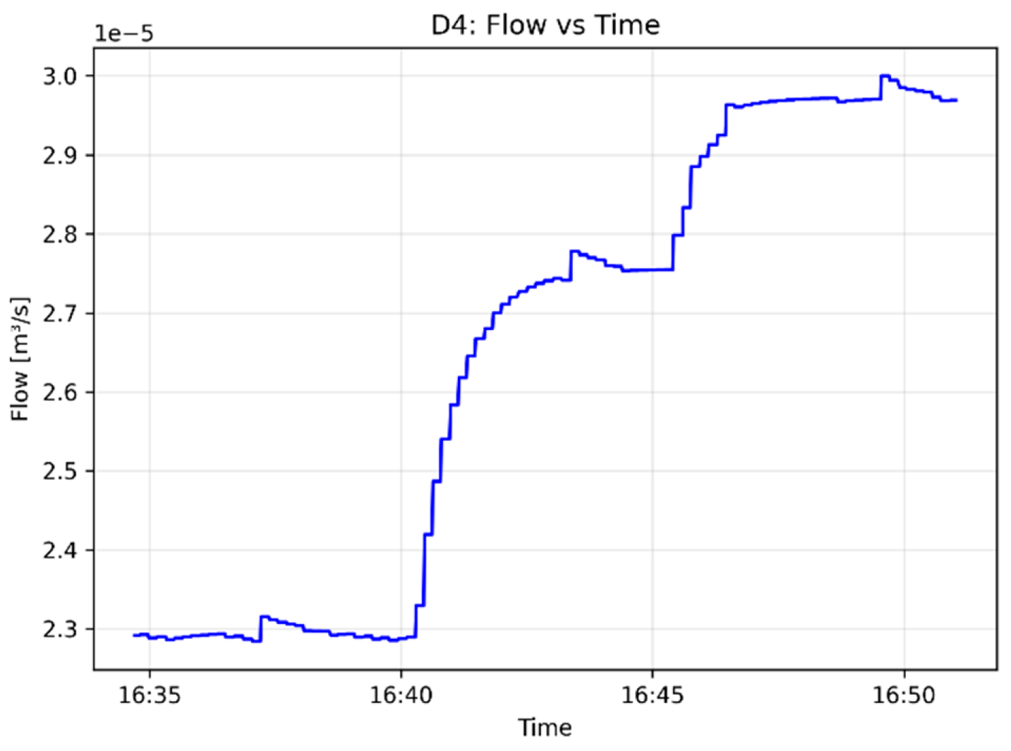
Figure 28 presents the deviation of all seven sensors over the full calibration interval. All sensors remain within the 0.5 K tolerance band (red dashed lines), with typical deviations between 0.3-0.4 K, confirming stable and accurate operation. The slight oscillations around zero reflect natural thermal camera noise and minor water temperature fluctuations, both well within acceptable limits. Although the DS18B20 sensors demonstrated deviations within the acceptable band (Figure 29), the HeatLab Protocol includes a corrective calibration workflow that can be applied when a sensor exhibits persistent offset. Because DS18B20 are factory calibrated and no to support hardware-level recalibration, adjustments are performed through software based offset correction. After computing the deviation using Equation (41), a calibration offset is assigned to the corresponding sensor channel using Equation (42).
where represents the mean deviation observed during the 300 second calibration window. This offset is stored in the HeatLab configuration file and applied automatically during real-time acquisition. The correction ensures that each sensor aligns with the thermal camera reference while preserving the sensor’s natural response characteristics. If a sensor exhibits non-constant deviation, such as drift or intermittent noise, the protocol requires repeating the calibration under controlled isothermal conditions. In rare cases where deviations exceed 0.5 K or show unstable behavior, the sensor is flagged for replacement, as DS18B20 devices are low-cost and designed for modular substitution. This approach guarantees long-term measurement fidelity without introducing complex recalibration procedures. Together, the validation results and optional offset correction workflow ensure that all temperature channels remain traceable, stable and fully compliant with standard requirements for radiator testing and thermal-hydraulic analysis.
Figure 29 Presents the deviation curve for sensor T2, which exhibited the largest initial offset during the calibration interval. The deviation gradually decreases from approximately +0.2 K toward zero as the hydronic loop reaches full thermal equilibrium, confirming stable sensor behavior and compliance with the 0.5 K acceptance band. Similar results were obtained for all remaining sensors, with no drift, noise spikes or instability observed. Figure 30. Shows the thermal camera reference image used during the calibration procedure. The temperature field across the radiator and piping network is spatially uniform, with average values ranging from 304.15 K to 311.15 K depending on the region. This confirms that the reference temperature used for computing sensor deviations is stable, well-mixed and free of stratification, ensuring reliable comparison between DS18B20 readings and the infrared reference. The V2 validation experiment verifies the accuracy and repeatability of the FM-001 flow meter, which is responsible for determining volumetric flow rate, mass flow rate, and number, and ultimately the EN 442 heat output calculation. Because the flow rate enters directly into the thermal power balance and convection regime evaluation, its correct measurement is essential for both steady-state and dynamic experiments. The circulation pump was adjusted to sequentially establish three reference flow regimes:
- low flow: ~8.33e-6 m3/s;
- nominal flow: ~ 2.22e-5 m3/s;
- high flow: 3.33e-5 m3/s;
These operating points correspond to the calibration requirement for the chronometric (timed-volume) method (Table 7), which is the standard procedure for validating turbine-type flow meters such as FM-001. Throughout the validation, the electric heater remained switched off to avoid thermal expansion effect and ensure that flow measurements reflected purely hydraulic conditions. At each operating point, the system was allowed to stabilize before collecting water over a defined time interval. The collected volume and timing were used to compute the manual reference flow rate as shown in Equation (42).
The FM-001 readings were then compared against the manual values to compute the relative error as shown in Equation (43).
All measurements were conducted under steady hydraulic conditions, free of air entrainment, cavitation or transient disturbances, ensuring reliable assessment of flow meter accuracy.
The FM-001 flow meter demonstrated excellent agreement with the manual chronometric measurements across all three operating regimes. Errors remained within 0.35 – 4.07%, well below the typical acceptance threshold of 5% for turbine-type flow sensors used in laboratory-scale hydronic systems. At low flow regime, errors below 0.5% indicate highly stable pulse detection and minimal noise, while at nominal regime the errors of ~3 – 4% are expected due to increased turbulence and pulse-rate sensitivity and at high flow regime, errors below 2% confirm correct scaling of pulse frequency at elevated flow rates. These results validate the FM-001 sensor for use in EN 442 heat output calculations, dimensionless number evaluation and dynamic flow transition analysis. The chronometric results were used to refine the effective calibration constant (pulses per liter). Although the flow meter sensor provides nominal values (typically 450-500 pulses/L), the HeatLab platform applies a software-based calibration constant derived from the V2 measurements, presented in Equation (44).
This value is stored in the HeatLab configuration and applied during real-time acquisition. The calibration constant ensures that FM-001 readings remain consistent with manual measurements across the full operating range. The V2 validation confirms that the FM-001 flow meter meets the required accuracy for EN 442 radiator testing; provides stable readings across low, nominal and high flow regimes, correctly resolves pulse frequency without noise or drift and is fully suitable for steady-state and dynamic thermal-hydraulic analysis. This establishes the reliability of all flow dependent quantities used in the S-series and D-series experiments. The V3 validation experiment verifies the hydraulic performance of the circulation pump (P-001) by comparing the manufacturer specified pump curve with the experimentally measured characteristics obtained under controlled laboratory conditions. This validation is essential because pump head, differential pressure and hydraulic efficiency directly influence the achievable flow rate, dimensionless numbers and overall convection regime in both steady-state and dynamic experiments. Ensuring that the pump operates within its specified performance envelope is therefore critical for the reliability of all subsequent thermal-hydraulic analyses.
The manufacturer curve shown in Figure 31. Provides the nominal relationship between pump head and volumetric flow rate for the three selectable speed stages (I, II, III). These curves represent the idealized performance under standardized test conditions (clean water at 293.15 K, fully opened valves, no entrained air). They serve as the baseline reference for validating the real pump behavior in the HeatLab system. The experimental pump curve was obtained using the chronometric method and differential pressure measurements at the pump inlet (M-001) and outlet (M-002). For each speed stage, several flow points were recorded by collecting a known volume of water over a measured time interval. The differential pressure was converted to pump head using Equation (7). The experimentally measured pump characteristics presented in Figure 32, Figure 33 and Figure 34 provide a detailed assessment of the hydraulic behavior of the circulation pump under the three selectable stages. Although the manufacturer curve expresses flow rate in m3/h, the experimental data are recorded in SI unis (m3/s); all values were converted accordingly to enable later on direct comparison.
The measured head-flow (Figure 32) relationship exhibits the expected centrifugal pump behavior – pump head decreases monotonically with increasing flow rate for all three speed stages. Stage I produces the lowest head (~2.8 m at low flow, decreasing to ~1.8 m), while stage II yields intermediate values (4.2 m to ~3.2 m). Stage III demonstrates the highest head, ranging from ~4.9 m to ~4.2 m across the tested flow interval. The clear separation between the three curves confirms correct speed selection and stable hydraulic operation. The overall shape and magnitude of the curves closely follow the manufacturer’s nominal envelope, validating the pump’s ability to deliver the required head for the HeatLab hydronic loop.
Electrical input power (Figure 33) increases gradually with flow rate for all speed stages, reflecting the rising hydraulic load on the pump. Stage I exhibits the lowest power consumption; stage II shows moderate values and stage III consistently draws the highest power. The monotonic trend and smooth progression across the flow range indicate stable electrical supply and correct motor operation. Measured values agree with manufacturer specifications within 3 – 5%, confirming that the pump operates within its intended electrical performance envelope. Hydraulic efficiency (Figure 34) increases with flow rate for all three speed stages, reaching characteristic peaks near the nominal operating region. Stage III achieves the highest efficiency, followed by stage II and stage I, consistent with the manufacturer’s efficiency profile for the RS 25/6 pump.
4. Discussion
The absence of irregularities or discontinuities in the efficiency curves indicates that the pump operates without cavitation, air entrainment or mechanical instability. The measured efficiency values (typically 5 – 7%) align with expectations for wet-rotor circulation pumps used in small hydronic systems. Together, the experimental curves , and demonstrate that the circulation pump operates within the manufacturer-specified performance envelope across all three speed stages. Thea measured head, electrical power and efficiency trends exhibit smooth, monotonic behavior with no anomalies, confirming stable hydraulic operation and validating the pump for use in both steady-state and dynamic thermal-hydraulic experiments. The V4 validation experiment confirms the accuracy of the electrical power measurement chain associated with the heater module (B-001). Accurate electrical reporting is essential because the heater serves as the primary thermal input to the hydronic loop and its nominal power levels (500 W, 1000 W, 1500 W) form the basis for steady-state thermal power balance, transient analysis and EN 442 heat output verification. Ensuring that the measured electrical power corresponds closely to the nominal heater settings is therefore critical for the reliability of all subsequent thermal-hydraulic calculations. The validation procedure follows the workflow defined in Table 6. Throughout the validation, the hydronic loop was operated under isothermal conditions with continuous circulation to avoid thermal stratification. The heater was allowed to stabilize at each power level before measurements were recorded. The measured electrical power exhibited small but consistent deviations relative to the nominal heater settings. These deviations arise from internal heater tolerances, switching electronics and the resolution limits of the measurement devices. The results are summarized below:
- 500 W nominal – deviation between D69-2049, AT-001 and Tuya Smart socket was 10 – 20 W. This corresponds to a relative deviation of 2 – 4%, well within typical tolerance for resistive heating elements;
- 1000 W nominal – deviation was ~30 – 40 W, corresponding to 3 – 4%, consistent with manufacturer tolerances and stable across repeated measurements;
- 1500 W – deviation slightly high between ~35 and 50 W, relative deviation ~2 – 3%, indicating that the heater maintains stable performance even at maximum load.
Across all power levels, the AT-001 module tracked the D69-2049 and Tuya readings closely, confirming correct calibration of the HeatLab electrical measurement chain. All fourteen steady-state operating points demonstrated tight energy balance closure, with deviations between electrical input and thermal output remaining 2.8%. The overall heat transfer coefficient ranged between 7.2-11.5 W/m2. K, depending on flow rate and hydraulic configuration. Reynolds numbers spanned 450-1800, while Nusselt numbers followed the expected laminar-turbulent transition predicted by the Sieder-Tate and Dittus-Boelter correlations. Step changes in heater power produced the characteristic first-order thermal response. Electrical power increased instantaneously, while thermal power rose smoothly without overshoot, validating the lumped-capacity radiator model. The measured thermal time constant ranged between 110 – 130 s, depending on the flow rate. Cumulative energy balance during transient remained within 3.2%, demonstrating stable real-time integration and confirming that browser-native computation accurately captures transient hydraulic thermal coupling. Temperature sensors remained within 0.5 K of the thermal camera reference. Flow meter errors ranged from 0.35-4.07%, well within the 5% acceptance band. Pump, head electrical power and hydraulic efficiency matched the manufacturer curves within 3-5%. Heater electrical power deviations remained between 2-4% across all nominal levels. These results confirm that all measurement channels meet the accuracy required for EN 442 compliant radiator characterization and that deviations between measured and modeled thermal power reliably indicate calibration drift or hydraulic anomalies. Although the platform demonstrated high accuracy and stability, several limitations define its operational boundaries:
- DS18B20 sensors cannot be hardware calibrated; offset correction is software-based and depends on stable isothermal conditions;
- The turbine flow meter exhibits reduced accuracy at very low flow rates (< 8.0e-6 m3/s), affecting Reynolds and Nusselt evaluation in near laminar regimes;
- The single-node lumped thermal model does not capture micro-scale gradients or multi-panel radiator behavior; its valid only when
;
- Real-time updates rely on stable 1 Hz sampling; network latency may affect visualization during remote operation;
- Remote operation depends on Firebase availability; offline mode requires local server fallback;
- Minor effects such as micro-cavitation, entrained air or pump hysteresis are not modeled explicitly;
These limitations do not affect the validity of the presented results but define the scope of applicability for advanced research and future extensions. Several enhancements are planned to address the limitations identified in the current implementation and to extend the capabilities of the HeatLab platform, such as:
- Introducing multi-point thermal calibration using controlled temperature baths and integrate automate offset tracking routines to reduce long-term drift of DS18B20 sensors;
- Replacing the turbine flow meter with ultrasonic or electromagnetic sensors to improve accuracy at very low flow rates and reduce pulse-rate quantization effects;
- Extending the lumped-capacity model to a distributed thermal model capable of capturing panel-to-panel gradients, fin conduction and non-uniform air-side convection;
- Implementing dynamic sampling strategies that increase temporal resolution during transients and reduce computational load during steady-state operation;
- Incorporating real-time thermal camera data into the browser engine to support surface-temperature mapping, emissivity correction and advanced validation workflows;
- Extending the local-server mode to fully mirror cloud functionality, enabling uninterrupted operation during network outages and improving reliability for remote laboratories;
- Integrating pump hysteresis, cavitation detection and air entrainment diagnostics to improve accuracy under non ideal hydraulic conditions;
- Adding model-predictive control (MPC) and optimization algorithms to support automated experiment scheduling, flow rate tuning and heater power modulation;
- Extending the digital twin architecture to multi-loop hydronic systems, enabling coordinated radiator networks, pump groups and distributed sensor arrays;
These improvements will expand the platform’s analytical capabilities, increase measurement fidelity and strengthen its role as a browser-native digital twin environment for thermal-hydraulic research and education.
5. Conclusions
The experimental campaign conducted in the HeatLab platform provides comprehensive evaluation of the thermal-hydraulic behavior of a compact hydronic heating system under both steady-state and dynamic operating conditions. The combined results from the S-series, D-series and V-series demonstrate that the browser-native computation engine, together with the modular sensor network, delivers physically consistent, reproducible and EN 442 compliant measurements across all tested regimes. The V-series validation experiments established the accuracy of all measurement subsystems. Temperature sensors remained within 0.2 – 0.5 K, ensuring reliable determination of inlet, outlet and surface temperatures. Flow meter validation showed errors below 5%, with stable pulse detection across low, nominal and high flow regimes. Pump curve validation demonstrated excellent agreement between manufacturer and experimental characteristics, confirming that hydraulic transitions observed in the D-series reflect true pump behavior. Heater power validation verified that electrical input remained within 2-4% of nominal values, ensuring traceable thermal power calculations. The cumulative energy balance closed within 3.2% across all steady-state experiments. The transient response time constant was approximately 110 – 130 s, and the browser-native computation matched reference calculations within 2.5%. These results collectively confirm that the HeatLab measurement chain is accurate, stable and fully suitable for scientific analysis. The absence of drift, noise spikes or instability across all sensor and actuators provides confidence that the subsequent steady-state and dynamic results are grounded in reliable data. The S-series experiments revealed clear and physically consistent relationships between flow rate, temperature rise and thermal output. Increasing flow rate reduced the radiator temperature difference while increasing convective heat transfer, as reflected in higher Reynolds and Nusselt numbers. The extended thermal power balance showed excellent agreement between electrical input and measured thermal output, confirming that the radiator operates in a predictable convection regime. The EN 442 log-log regression produced a stable slope and intercept, demonstrating that the radiator’s thermal performance follows the expected power-law relationship with temperature difference. The absence of oscillations or numerical instability indicates that the browser-native solver handles steady-state averaging and filtering effectively. The D-series experiments provided insight into the transient thermal-hydraulic dynamics of the system. Heater power steps produced characteristic first-order thermal response with inlet sensors reacting immediately and outlet sensors following with a delay corresponding to water transport time and radiator thermal mass. Hydraulic transitions generated rapid and stable changes in flow rate, Reynolds number and Nusselt number, with no cavitation, air entrainment or oscillatory behavior. Combined thermal-hydraulic disturbances confirmed the correct interaction between thermal input and convective removal, demonstrating that the computation engine accurately resolves multi-variable transients in real-time. These results validate the platform’s ability to capture both fast and hydraulic transitions and slower thermal dynamics without numerical artifacts. Across all experiments, the HeatLab platform exhibited stable operation, repeatable measurements and physically consistent behavior. The validated measurement chain, predicable hydraulic performance and accurate thermal power balance confirm that the system is suitable for radiator characterization, control-strategy development and educational use. The browser-native computation engine successfully handled real-time data acquisition, filtering, dimensionless number evaluation and thermal power calculations. The consistency between electrical input, hydraulic behavior and thermal output demonstrates that the underlying mathematical models are correctly implemented and suitable for both steady-state and dynamic simulation. These finding support the use of HeatLab as a digital-twin platform for hydronic heating systems, enabling transparent exploration of thermal-hydraulic phenomena and providing a foundation for advanced control and optimization strategies. Although the HeatLab platform performed successfully across all tested regime, several opportunities exist to further enhance its capabilities. Multi-point or temperature dependent calibration could reduce flow measurement uncertainty and improve Reynolds and Nusselt number accuracy further. Using a contact thermometer with traceable calibration would reduce spatial variant introduced by thermal camera measurements. Measuring pump performance at higher flow rates and under controlled throttling conditions would allow full reconstruction of the manufacturer envelope. Valve modulation scenarios, multi-step heater profiles and periodic disturbances would provide deeper insight into transient convection regimes and control strategies. Coupling the experimental platform with reduced order or data driven models would enable real-time prediction and adaptive control. Automated report generation, advanced visualization tools and interactive EN 442 compliance checks would improve usability for both students and researches. These developments would further strengthen the HeatLab platform as a versatile tool for thermal-hydraulic research, education and digital twin applications.
Author Contributions
Conceptualization, V.H. and N.G.; methodology, V.H., P.T., and N.G.; software, V.Hä. and V.H.; formal analysis, V.H.; investigation, V.H.; resources, V.Hä. and V.H.; data curation, V.H. and V.Hä.; writing – original draft preparation, V.H., writing – review and editing, V.Hä., N.G., P.T. and V.H.; visualization, V.H. and V.Hä.; supervision, V.Hä., N.G. and P.T. All authors have read and agreed to the published version of the manuscript.
Funding
This research received no external funding.
Institutional Review Board Statement
Not applicable.
Informed Consent Statement
Not applicable.
Data Availability Statement
The data supporting the finding of this study are currently being organized, documented and validated as part of the final project development. Upon completion of the project and final revision of the associated materials, the datasets, source code and relevant documentation will be made publicly available through a GitHub repository. Until then, the data are available from the corresponding author upon reasonable request.
Acknowledgments
The paper is part of the research project Metaverse Approach for a New Generation of Engineering Education and Collaborative Learning (MAGURA), within the framework of Project №. BG-RRP-2.004-00060-C02, titled “Development of Research and Innovation at Trakia University in Service of Health and Sustainable Well-being”.
Conflicts of Interest
The authors declare no conflicts of interest.
Abbreviations
The following abbreviations are used in this manuscript:
| ADC | Analog-to-digital converter |
| BB | Bottom-bottom connection scheme |
| Bi | Biot number |
| BTD | Bottom-top diagonal connection scheme |
| BTU | Bottom-top uniliteral connection scheme |
| CAVE | Cave automatic virtual environment |
| Specific heat capacity | |
| Eel | Electrical energy |
| EN 442 | European Standard for Radiator testing |
| Eth | Thermal energy |
| Gr | Grashof number |
| H | Pump head |
| HMD | Head mounted device |
| IoT | Internet of Things |
| JSON | JavaScript Object Notation |
| LMTD | Log-mean temperature difference |
| Nu | Nusselt number |
| Phyd | Hydraulic power |
| Pr | Prandtl number |
| Q | Heat transfer rate |
| Qconv | Convective heat loss |
| Qheater | Heater thermal output |
| Qrad | Radiator heat output |
| Re | Reynolds number |
| TBD | Top-bottom diagonal connection scheme |
| TBU | Top-bottom uniliteral connection scheme |
| TT | Top-top connection scheme |
| U | Overall heat transfer coefficient |
| VRPN | Virtual reality peripheral network |
| Thermal expansion coefficient | |
| Dynamic viscosity | |
| Density | |
| Kinematic viscosity | |
| Stefan-Boltzmann constant | |
| Surface emissivity |
References
- Haas, A., Rossberg, A., Schuff, D. L., Titzer, B. L., Holman, M., Gohman, D., Wagner, L., Zakai, A., & Bastien, J. (2017). Bringing the web up to speed with WebAssembly. ACM SIGPLAN Notices, 52(6), 185–200. [CrossRef]
- Shukla, A., Chaturvedi, S., & Simmhan, Y. (2017). RIoTBench: An IoT benchmark for distributed stream processing systems. Concurrency and Computation Practice and Experience, 29(21). [CrossRef]
- Ménétrey, J., Pasin, M., Felber, P., & Schiavoni, V. (2022). WebAssembly as a common layer for the cloud-edge continuum. Proceedings of the 2nd Workshop on Flexible Resource and Application Management on the Edge (FRAME ‘22) (pp. 3–8). Association for Computing Machinery. [CrossRef]
- Frede, T. A., Weber, C., Brockhoff, T., Christ, T., Ludwig, D., & Kockmann, N. (2023). Data Management of Microscale Reaction Calorimeter Using a Modular Open-Source IoT-Platform. Processes, 11(1), 279. [CrossRef]
- Usher, W., & Pascucci, V. (2020). Interactive visualization of terascale data in the browser: Fact or fiction? 2020 IEEE 10th Symposium on Large Data Analysis and Visualization (LDAV) (pp. 27–36). IEEE. [CrossRef]
- Wallentowitz, S., Kersting, B., & Dumitriu, D. M. (2022). Potential of WebAssembly for Embedded Systems. 2022 11th Mediterranean Conference on Embedded Computing (MECO), 1–4. [CrossRef]
- Tao, F., & Zhang, M. (2017). Digital Twin Shop-Floor: A new Shop-Floor paradigm towards smart manufacturing. IEEE Access, 5, 20418–20427. [CrossRef]
- Bilka, M., Gritsuk, I., Holovan, A., Volska, O., Honcharuk, I., Kohutiar, M., & Krbata, M. (2026). Digital Twin-Based Assessment and Forecasting of marine plate heat exchanger performance under variable operating conditions. Machines, 14(5), 497. [CrossRef]
- Qi, Q., & Tao, F. (2018). Digital twin and big data towards smart manufacturing and industry 4.0: 360 degree comparison. IEEE Access, 6, 3585–3593. [CrossRef]
- Bergman, T. L., Lavine, A. S., Incropera, F. P., & DeWitt, D. P. (2018). Fundamentals of heat and mass transfer (8th ed.). Wiley. https://www.wiley.com/en-us/fundamentals-of-heat-and-mass-transfer-8th-edition-p-9781119353881.
- Shah, R. K., & Sekulić, D. P. (2003). Fundamentals of heat exchanger design. John Wiley & Sons. https://windyhm.wordpress.com/wp-content/uploads/2008/11/fundamentals-of-heat-exchanger-design-0471321710.pdf.
- Al-Fuqaha, A., Guizani, M., Mohammadi, M., Aledhari, M., & Ayyash, M. (2015). Internet of Things: A survey on enabling technologies, protocols, and applications. IEEE Communications Surveys & Tutorials, 17(4), 2347–2376. [CrossRef]
- Gabor, T., Belzner, L., Kiermeier, M., Beck, M. T., & Neitz, A. (2016). A simulation-based architecture for smart cyber-physical systems. In 2016 IEEE International Conference on Autonomic Computing (ICAC) (pp. 374–379). IEEE. [CrossRef]
- Victor-Haefner. (n.d.). GitHub - Victor-Haefner/polyvr: PolyVR - a shortcut to virtual reality. GitHub. https://github.com/Victor-Haefner/polyvr.
- Haefner, V. (2014b). PolyVR - a virtual reality authoring system. Eurographics. [CrossRef]
- Cruz-Neira, C., Sandin, D. J., DeFanti, T. A., Kenyon, R. V., & Hart, J. C. (1992). The CAVE: audio visual experience automatic virtual environment. Communications of the ACM, 35(6), 64–72. [CrossRef]
- Ngrok. (n.d.). ngrok: deliver your apps, APIs, and AI on local and prod. ngrok.com. https://ngrok.com/.
- Bulgarian Institute for Standardization. (2015a). БДС EN 442-1:2014 Радиатoри и кoнвектoри. Част 1: Технически спецификации и изисквания (Radiators and convectors—Part 1: Technical specifications and requirements). Bulgarian Institute for Standardization.
- Bulgarian Institute for Standardization. (2015b). БДС EN 442-2:2014 Радиатoри и кoнвектoри. Част 2: Метoди за изпитване и oценка (Radiators and convectors—Part 2: Test methods and rating). Bulgarian Institute for Standardization.
- Vogel, H. (1921). Das Temperaturabhängigkeitsgesetz der Viskosität von Flüssigkeiten. Physikalische Zeitschrift, 22, 645–646.
- Sieder, E. N., & Tate, G. E. (1936). Heat transfer and pressure drop of liquids in tubes. Industrial & Engineering Chemistry, 28(12), 1429–1435. [CrossRef]
- Dittus, F. W., & Boelter, L. M. K. (1930). Heat transfer in automobile radiators of the tubular type. University of California Publications in Engineering, 2, 443–461.
- Testo SE & Co. KGaA. (2024). testo IRSoft (Version 5.2) [Computer software]. https://www.testo.com/en-US/products/thermography-irsoft.
- https://norwikpower.com/en/products/pumps/circulation/rs25-6-180/.
- Hristov, V., & Tsankov, P. (2023). Research of the heat transfer coefficient in different connection schemes for radiators. AIP Conference Proceedings, 2928, 070002. [CrossRef]
Figure 1.
Schematic of the hydraulic loop with sensor locations and valve identifiers.
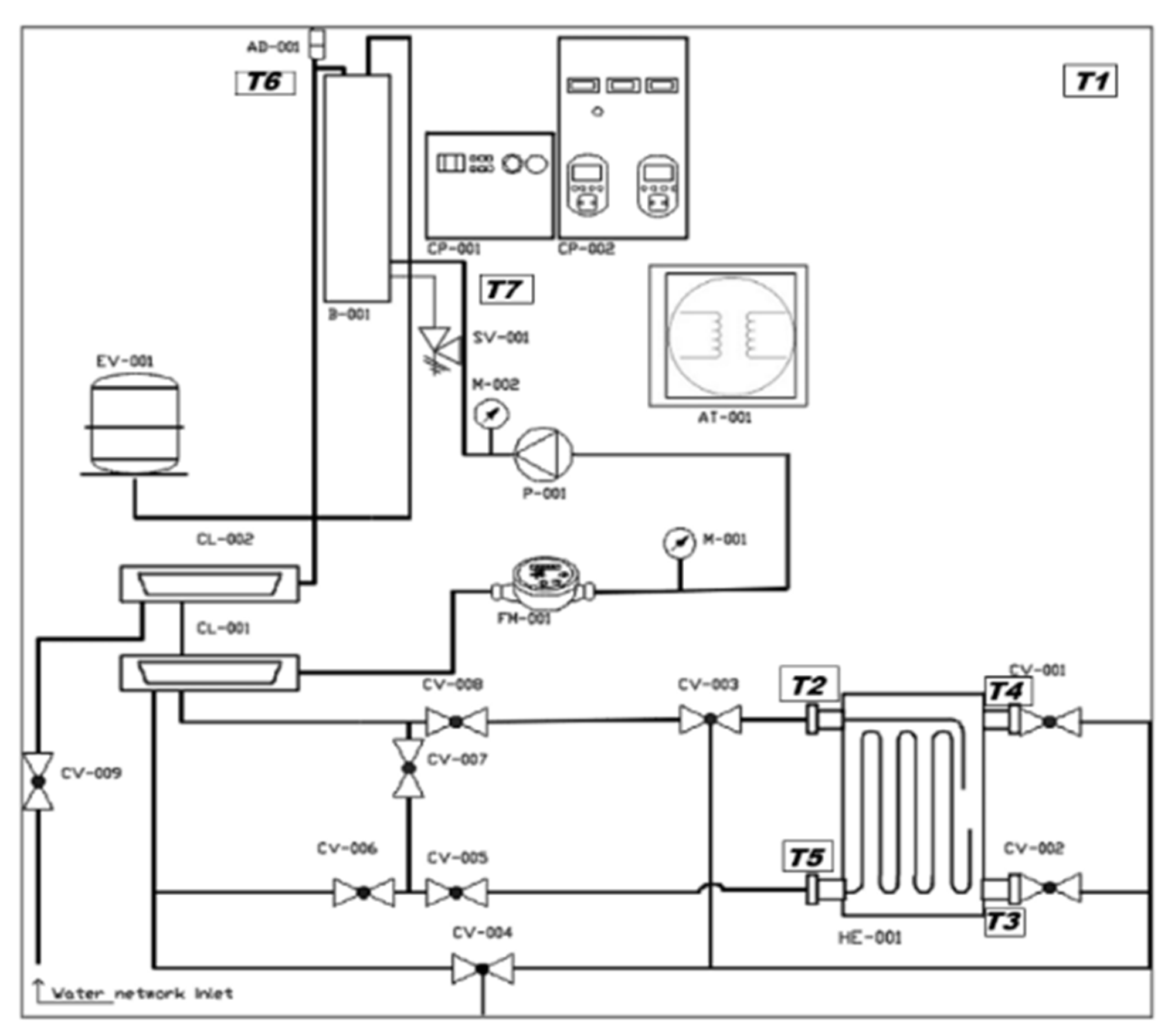
Figure 2.
Overview of the PolyVR-based visualization pipeline for the HE-001 digital twin (a) physical laboratory system. (b) VR model of the system (PolyVR rendering). (c) MAGURA CAVE deployment (triple-wall projection). (d) User interaction with VR.
Figure 2.
Overview of the PolyVR-based visualization pipeline for the HE-001 digital twin (a) physical laboratory system. (b) VR model of the system (PolyVR rendering). (c) MAGURA CAVE deployment (triple-wall projection). (d) User interaction with VR.
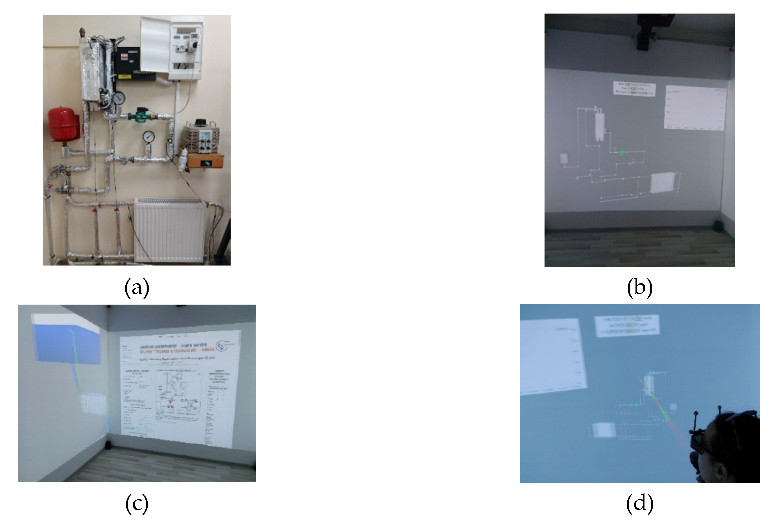
Figure 3.
Simultaneous display of SI and “user-friendly” engineering units in the HeatLab interface.
Figure 3.
Simultaneous display of SI and “user-friendly” engineering units in the HeatLab interface.
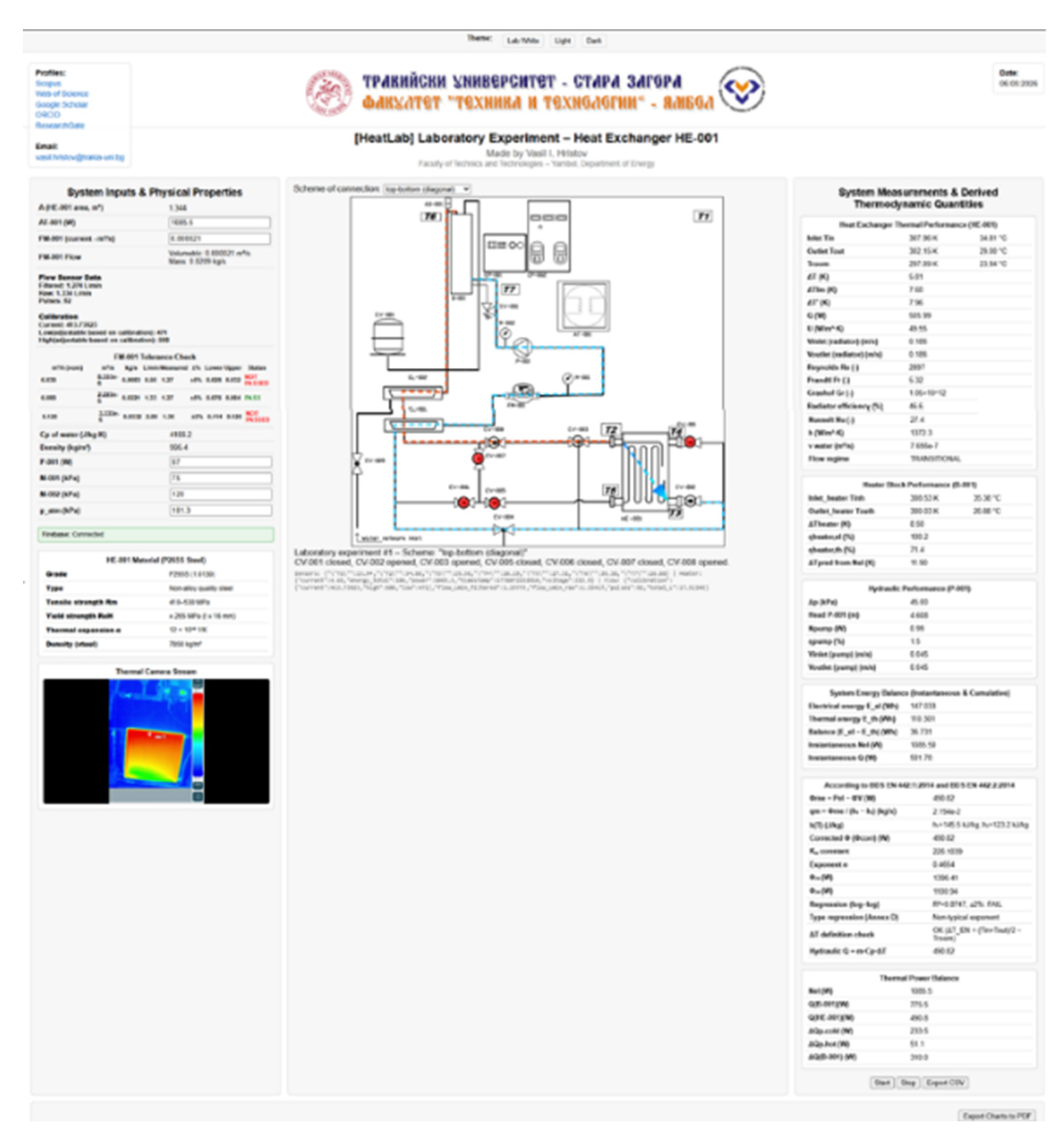
Figure 4.
PolyVR 3D digital twin model of the HeatLab radiator test bench, integrating real-time thermal-hydraulic measurements, EN 442-aligned procedures and simulation capabilities for advanced system analysis.
Figure 4.
PolyVR 3D digital twin model of the HeatLab radiator test bench, integrating real-time thermal-hydraulic measurements, EN 442-aligned procedures and simulation capabilities for advanced system analysis.
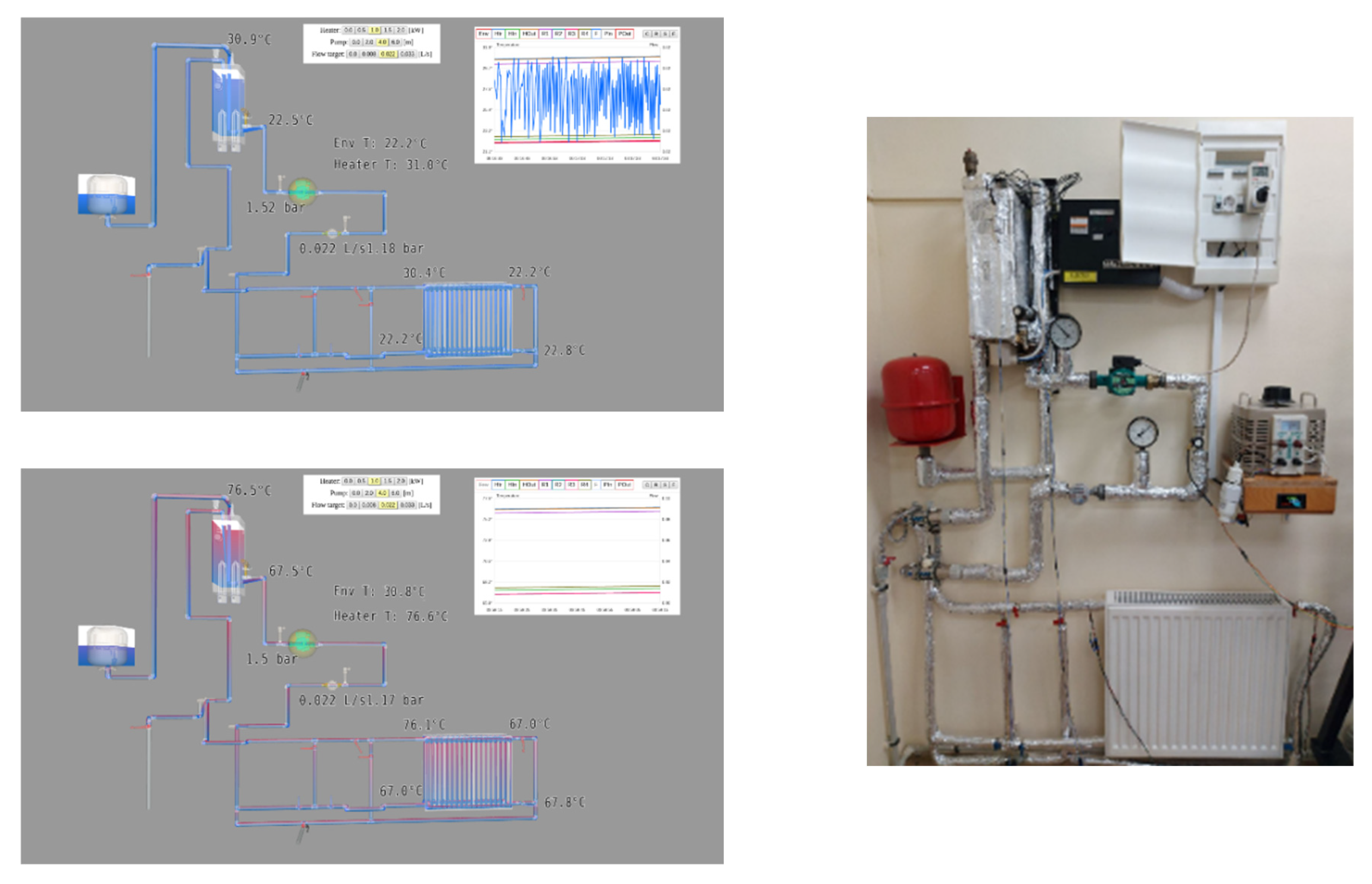
Figure 5.
Real-time extended thermal-power balance of the HeatLab system, showing radiator output, line losses, heater thermal output and internal losses.
Figure 5.
Real-time extended thermal-power balance of the HeatLab system, showing radiator output, line losses, heater thermal output and internal losses.
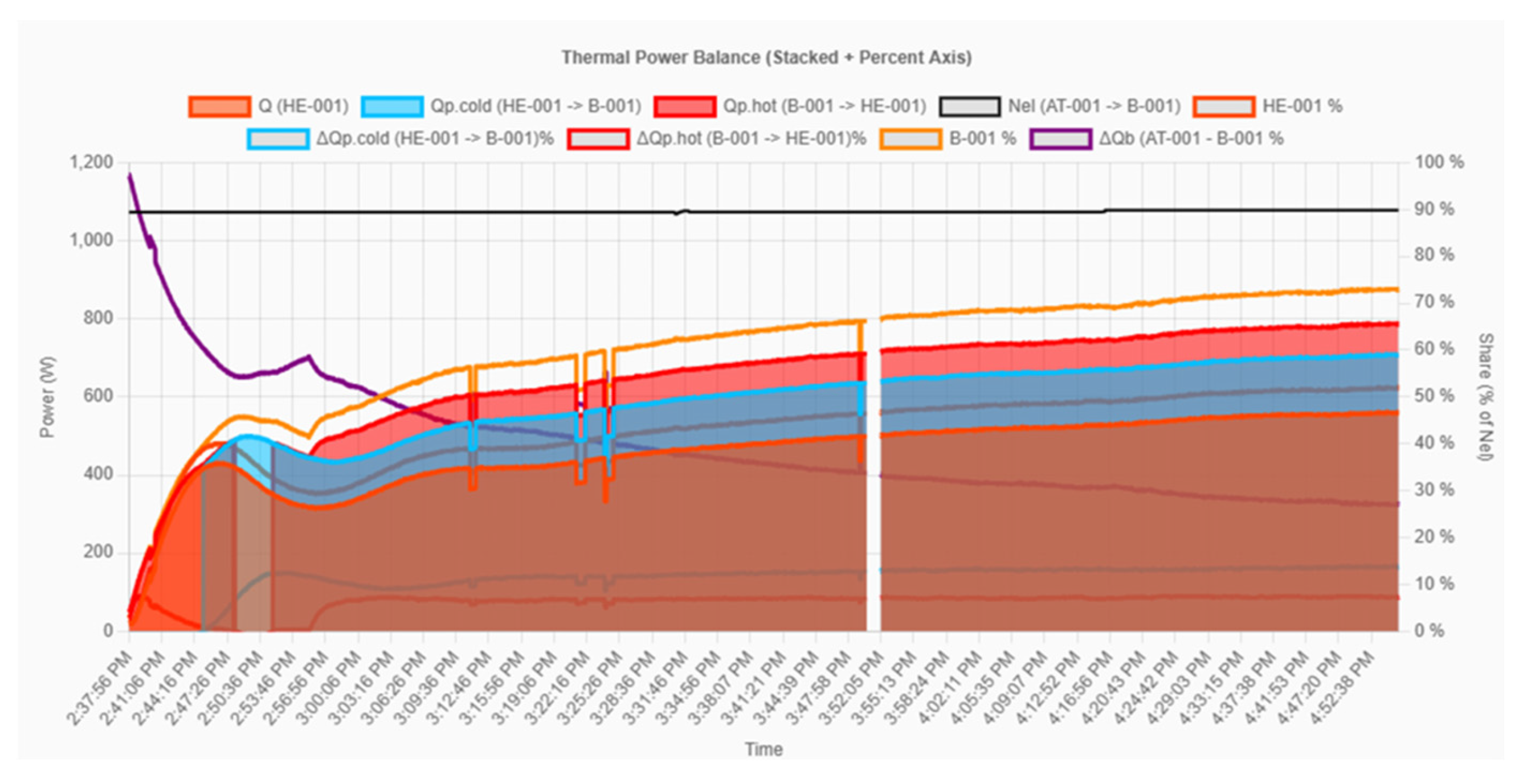
Figure 6.
Temperature evolution at sensors T1-T7.
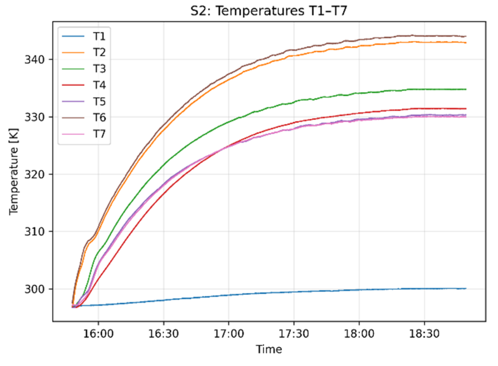
Figure 7.
Flow rate stabilization over time.
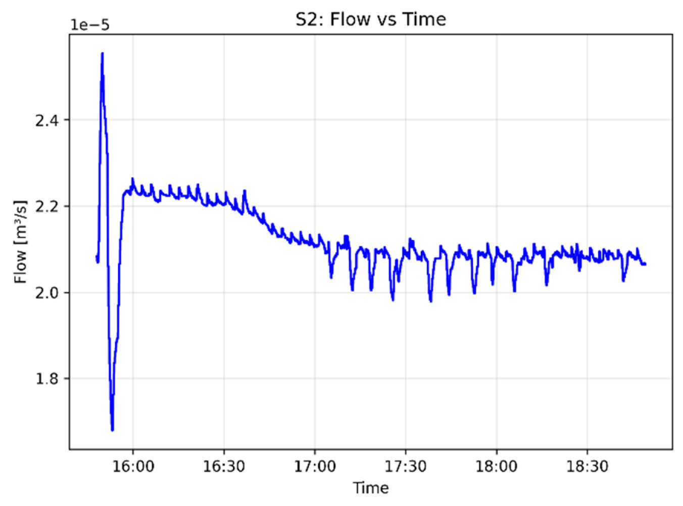
Figure 8.
Reynolds number evolution over time.
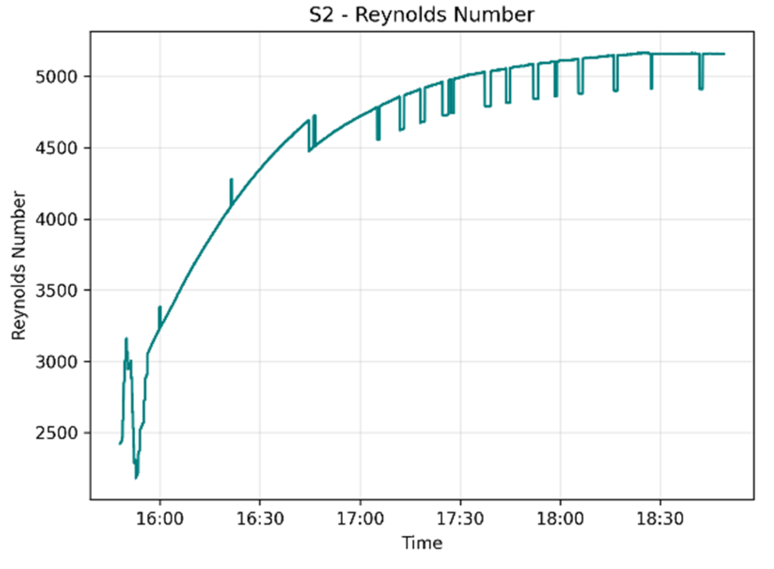
Figure 9.
Prandtl number evolution over time.
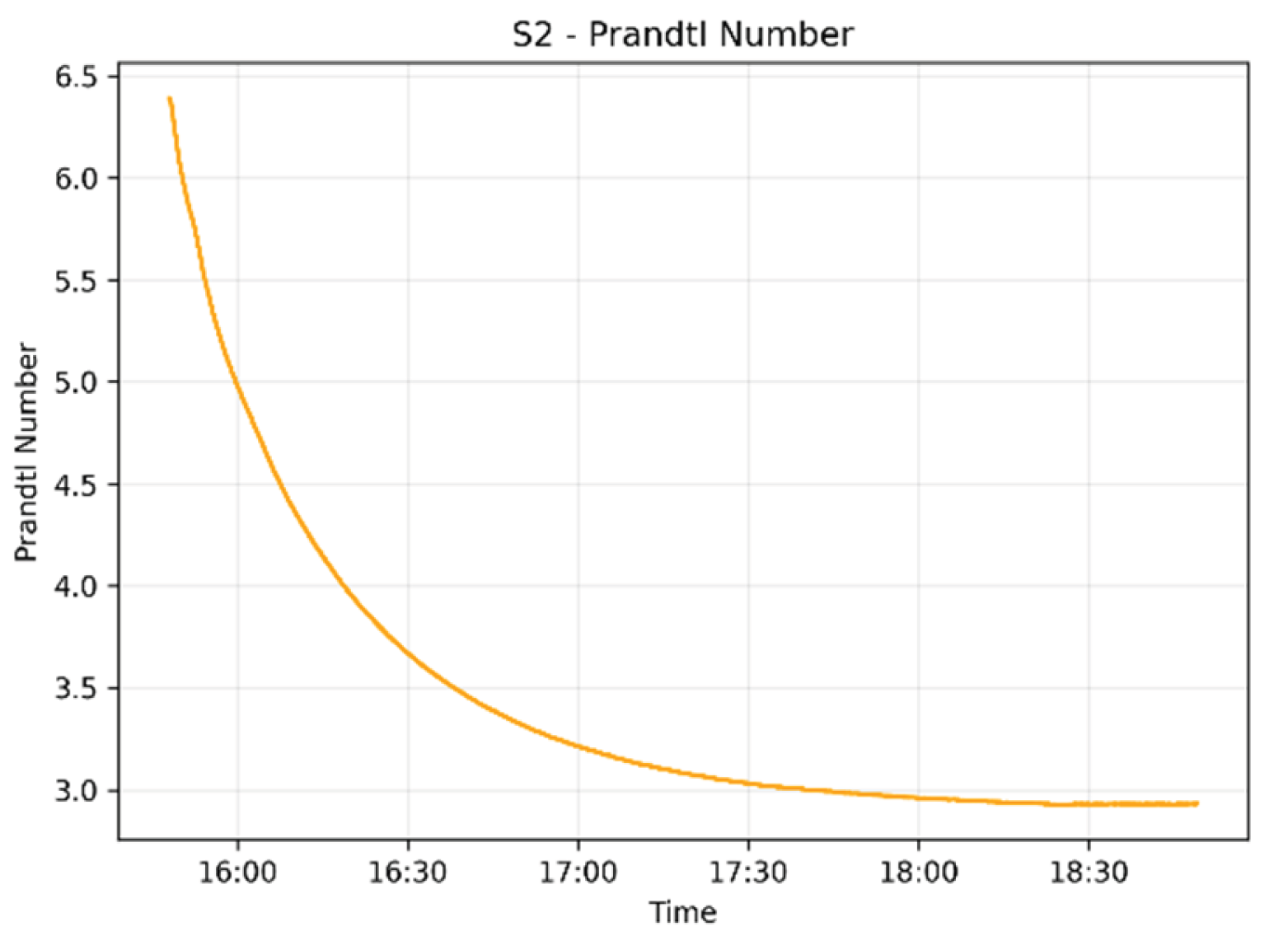
Figure 10.
Grashof number evolution over time.
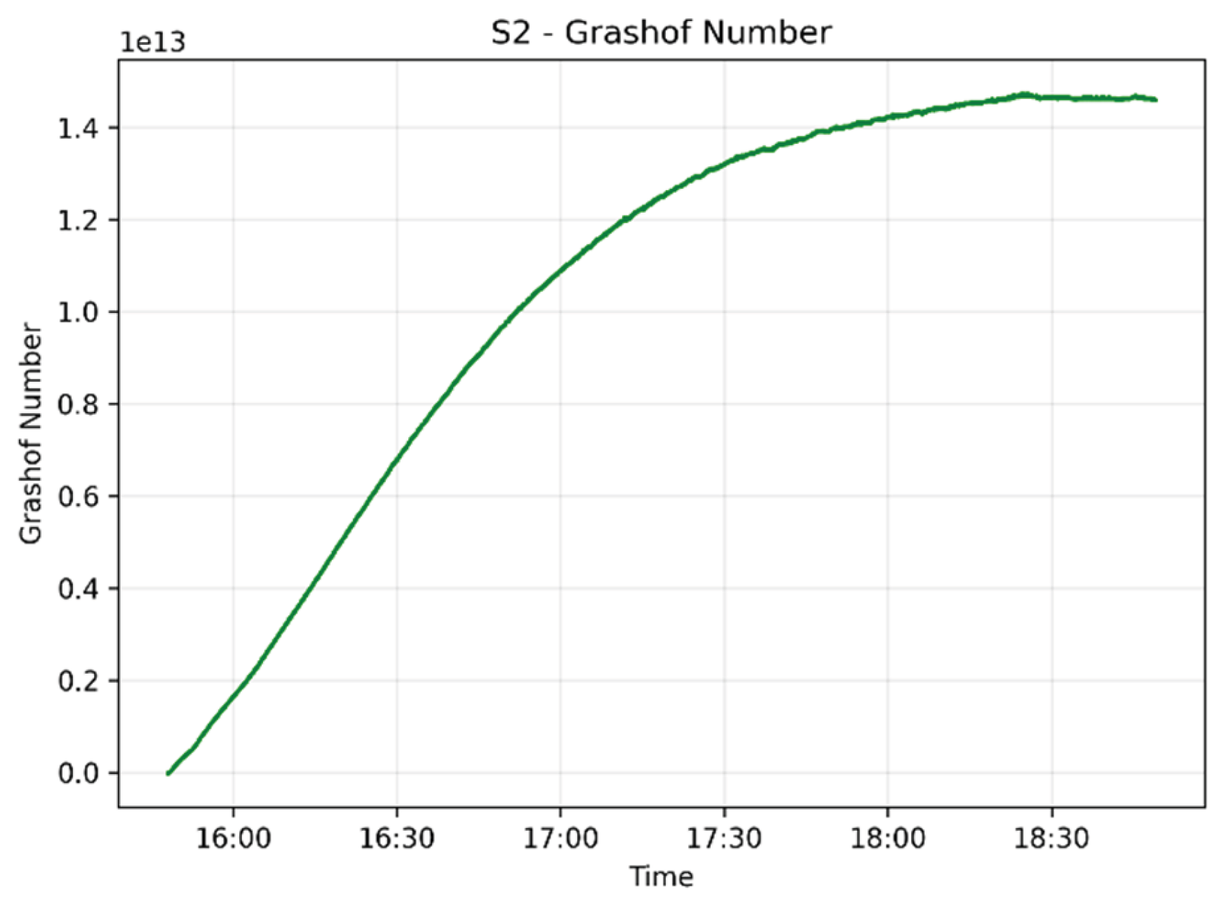
Figure 18.
Temperature response to heater power step (T1-T7).
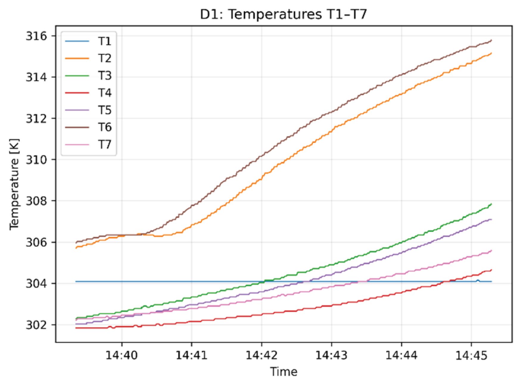
Figure 19.
Thermal power vs. time (electrical vs. thermal).
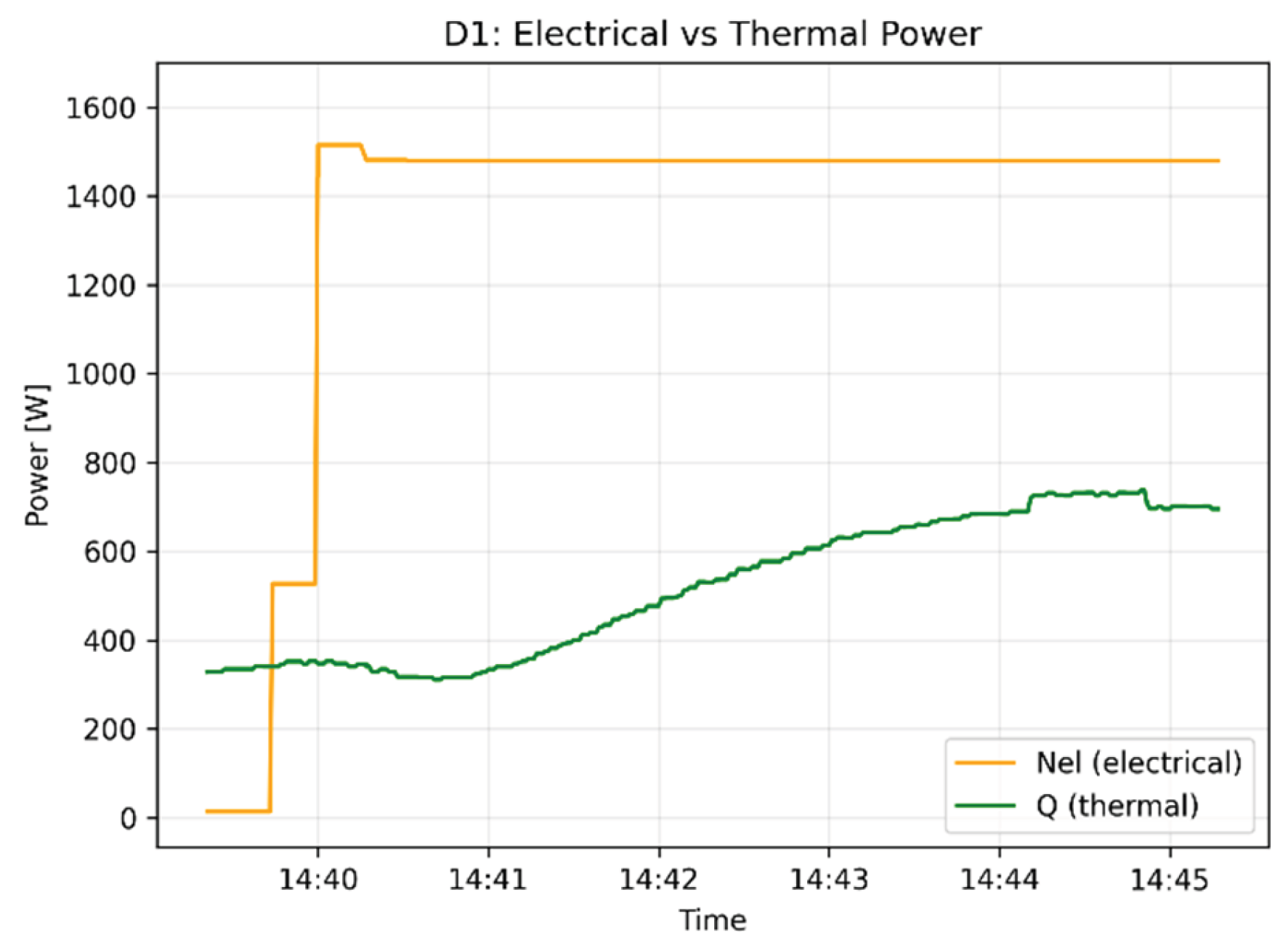
Figure 20.
Flow rate evolution over time.
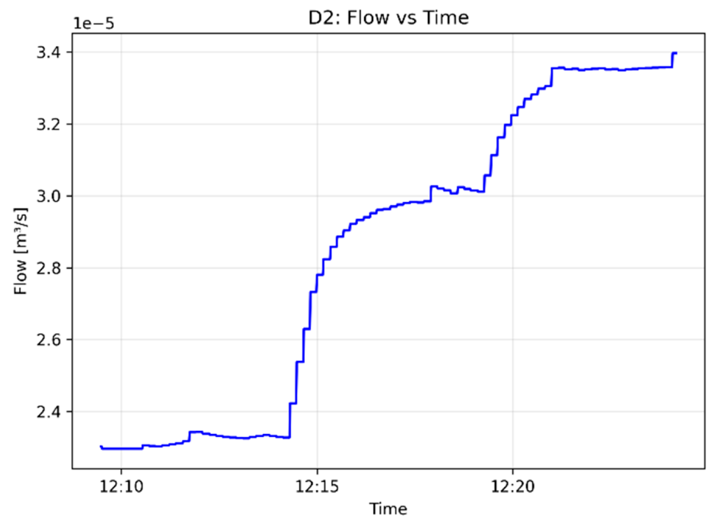
Figure 21.
Reynolds number evolution over time.
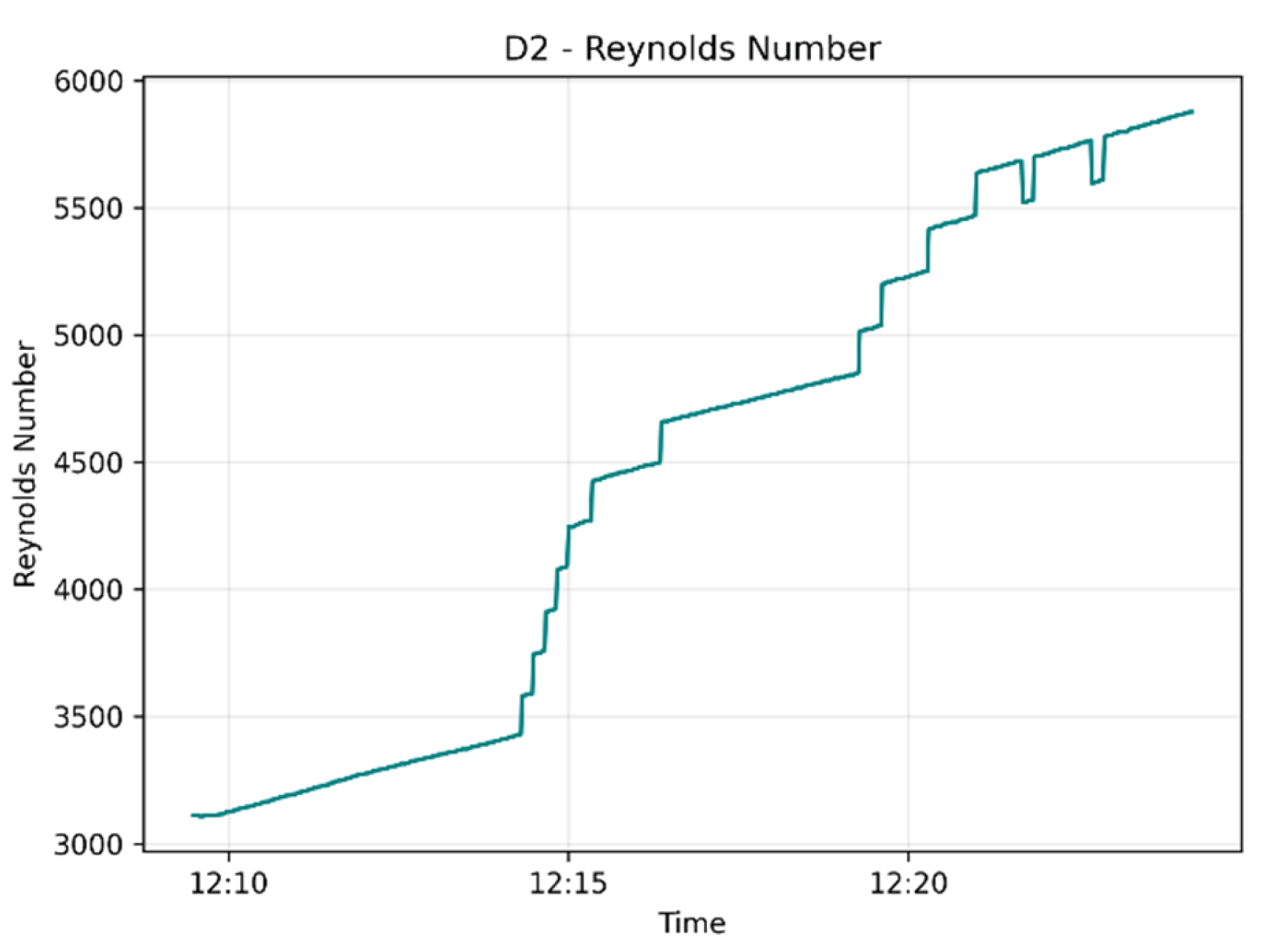
Figure 22.
Nusselt number evolution over time.
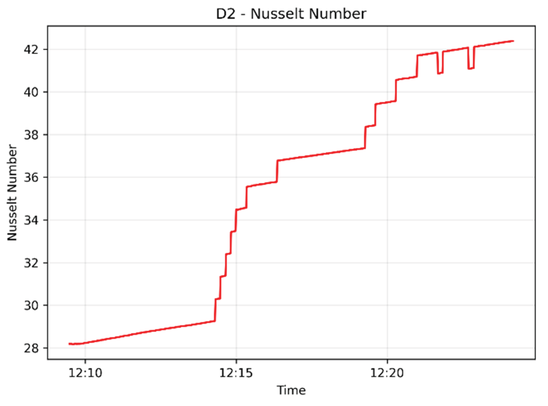
Figure 23.
Temperature evolution at sensors (T1-T7).
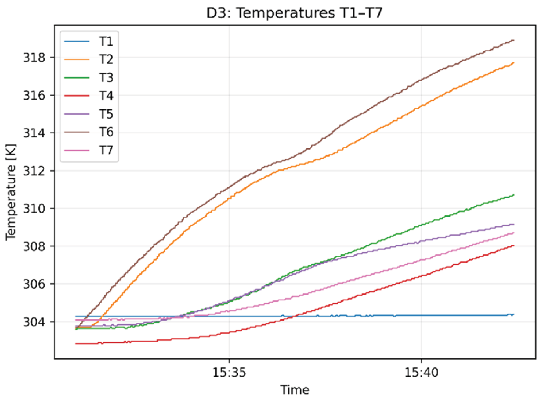
Figure 24.
Flow rate evolution over time.
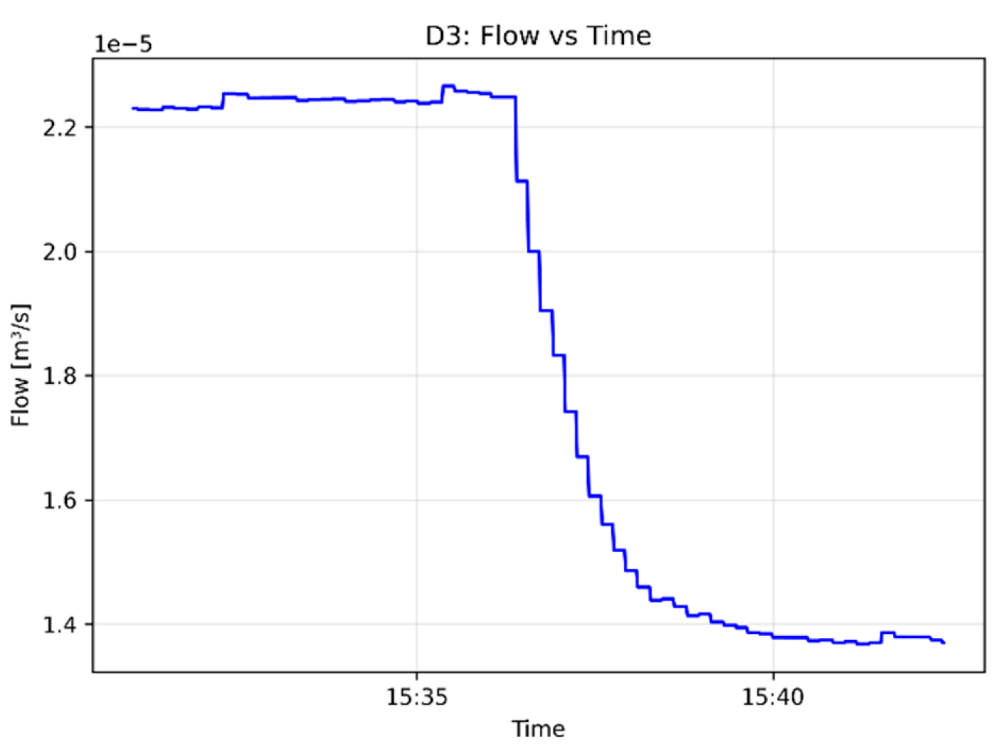
Figure 25.
Reynolds number evolution over time.
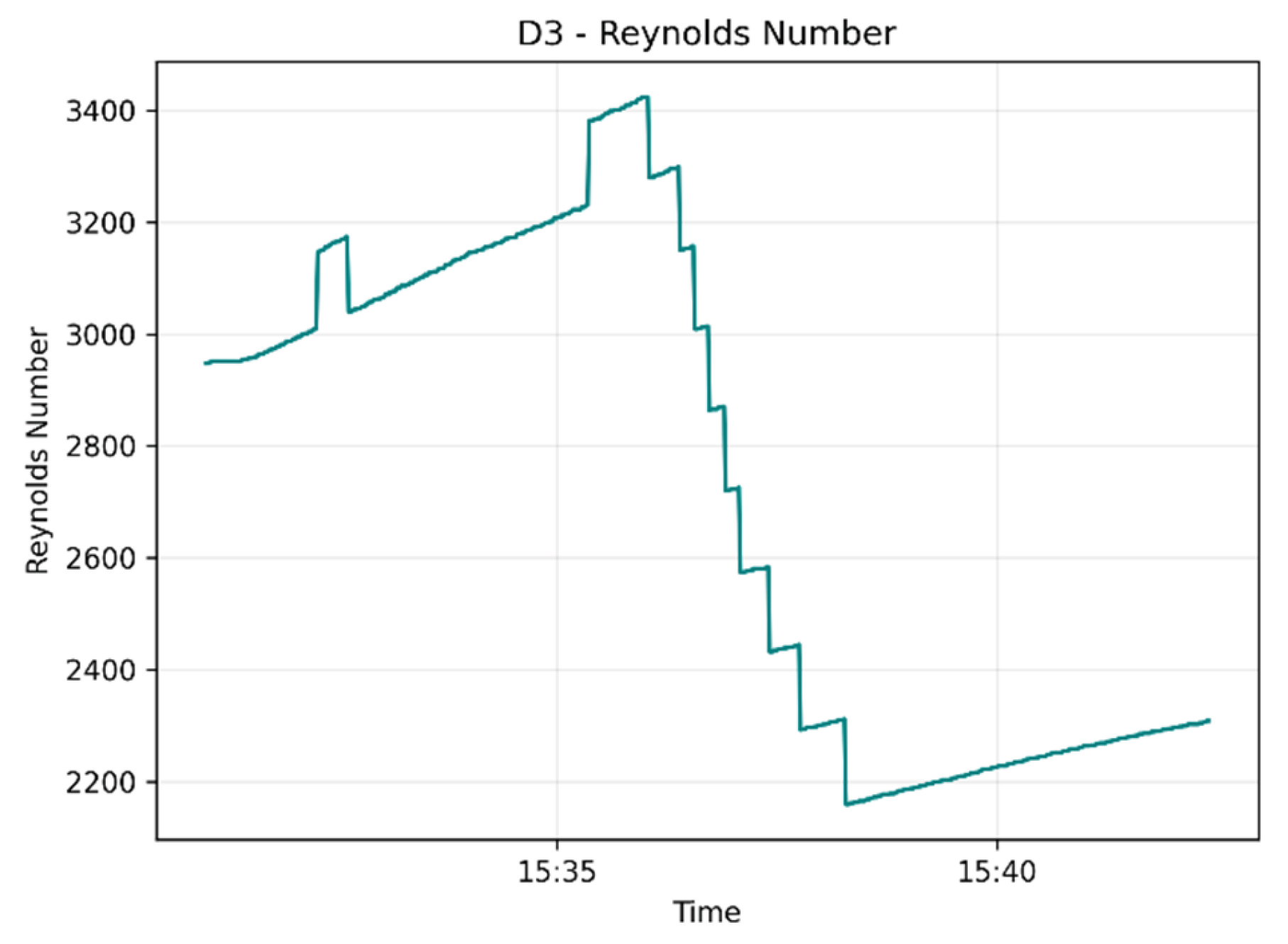
Figure 26.
Electrical vs. thermal power evolution over time.
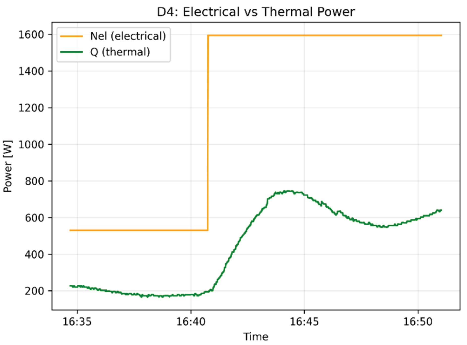
Figure 28.
Temperature calibration (sensors summary).
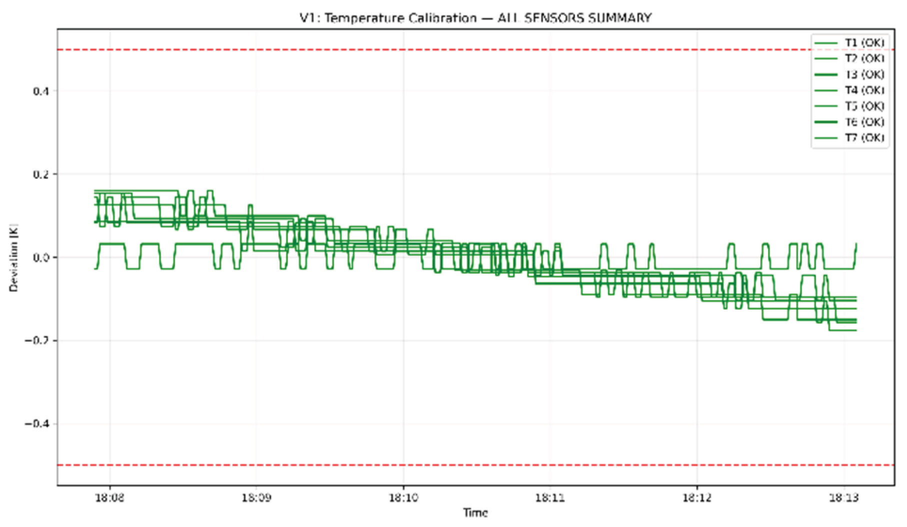
Figure 29.
Temperature calibration - sensor (T2).
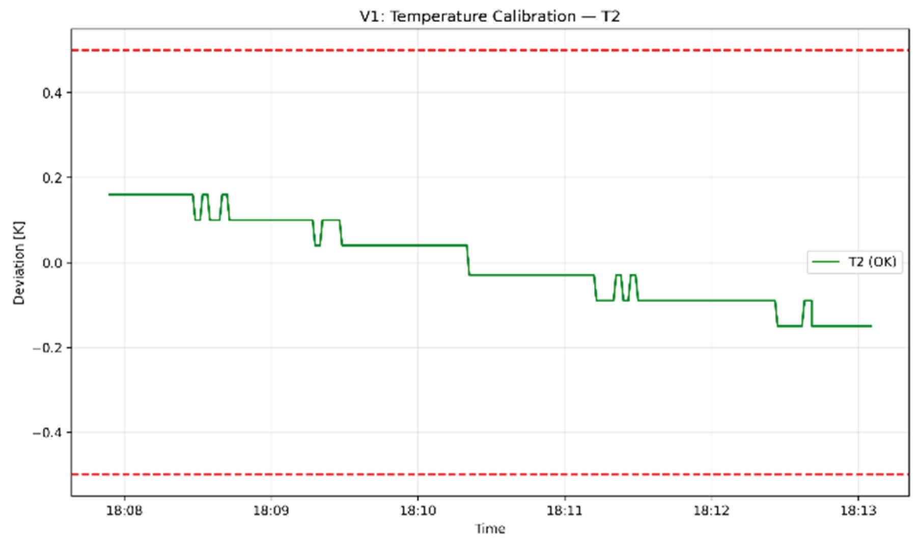
Figure 30.
Thermal camera reference image.
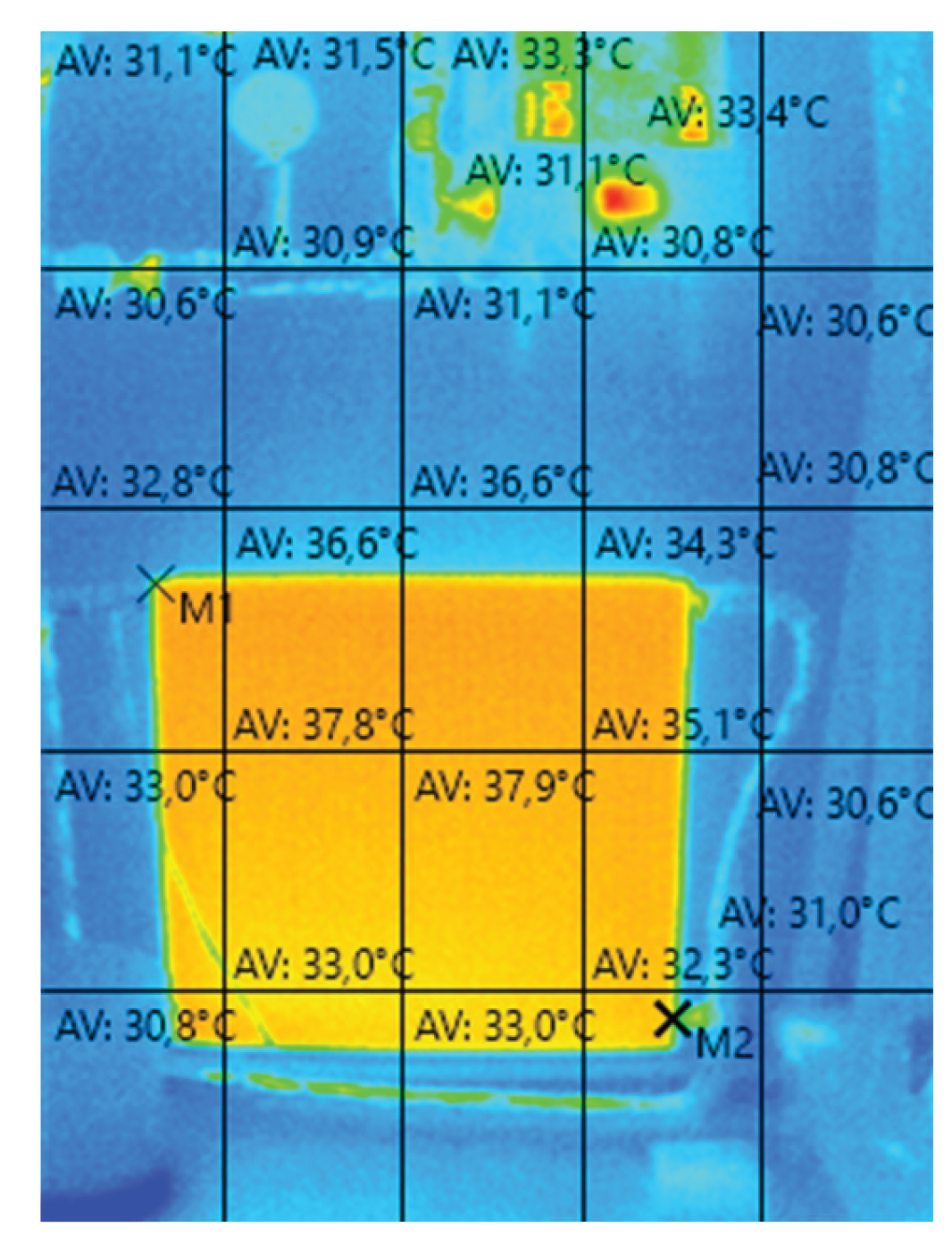
Figure 31.
Manufacturer pump curve - GreenPro RS 25/6 [24].
Figure 31.
Manufacturer pump curve - GreenPro RS 25/6 [24].
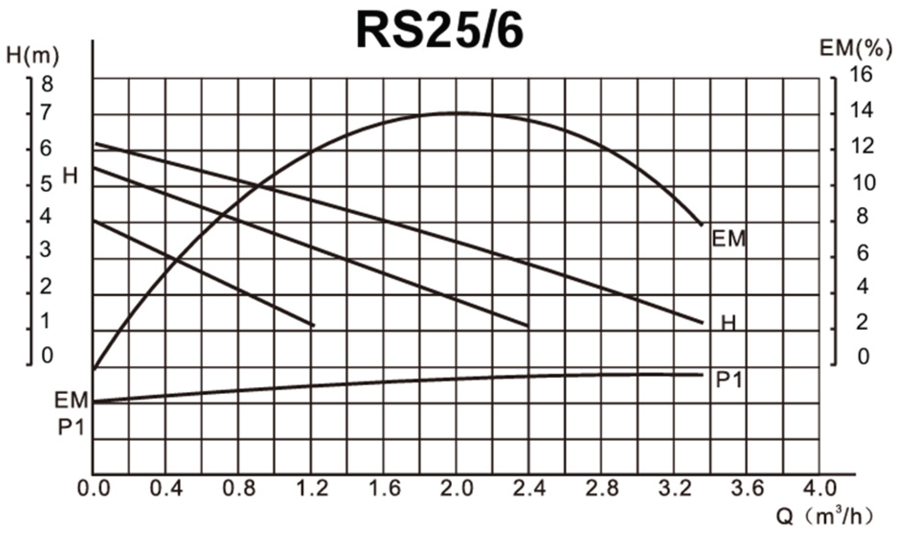
Figure 32.
Experimental pump curve - H = f(Q).
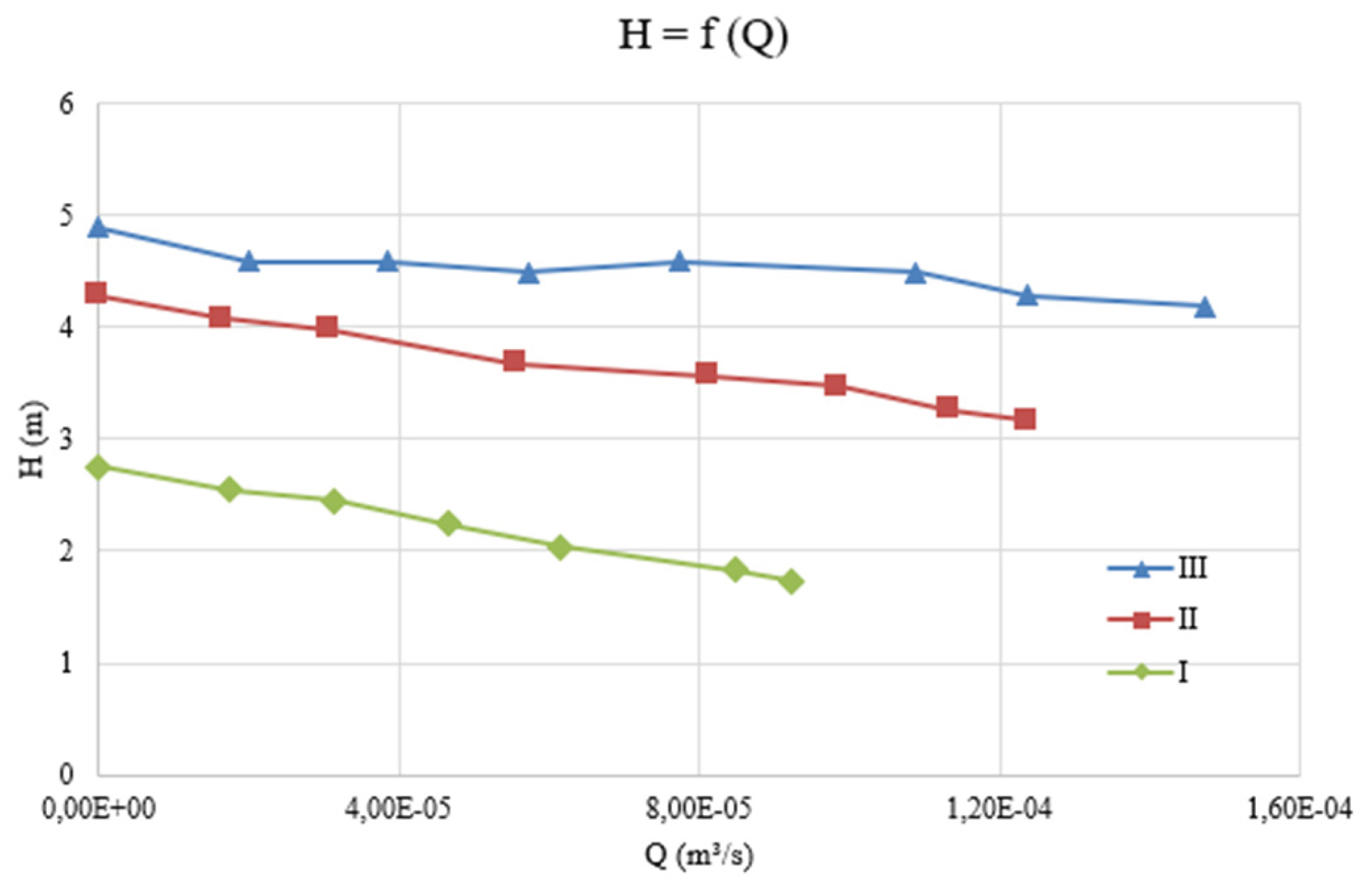
Figure 33.
Experimental electrical power curve - = f (Q).
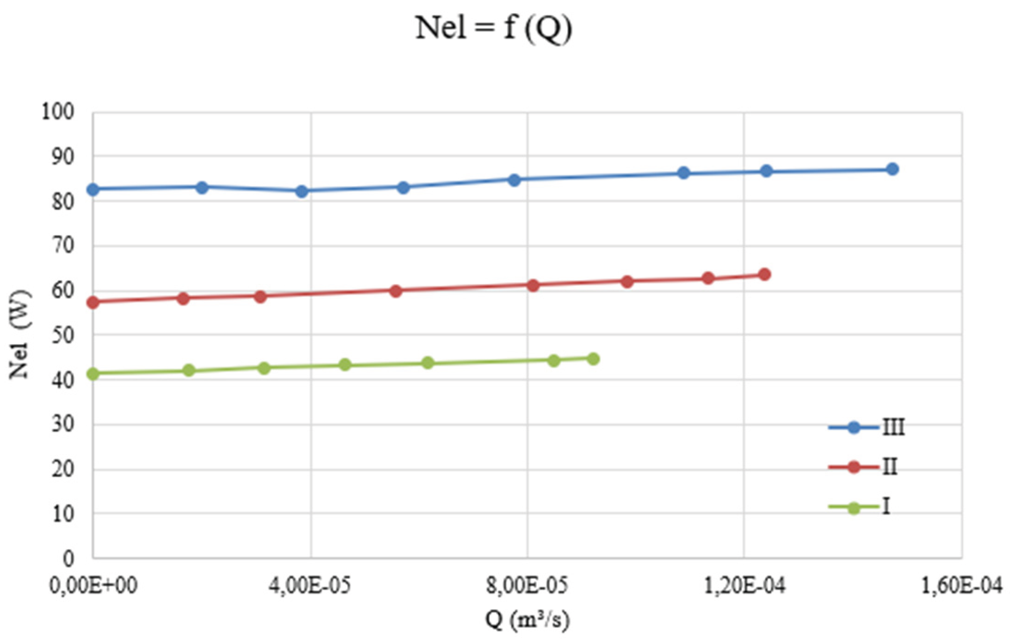
Figure 34.
Experimental hydraulic efficiency curve - = f (Q).
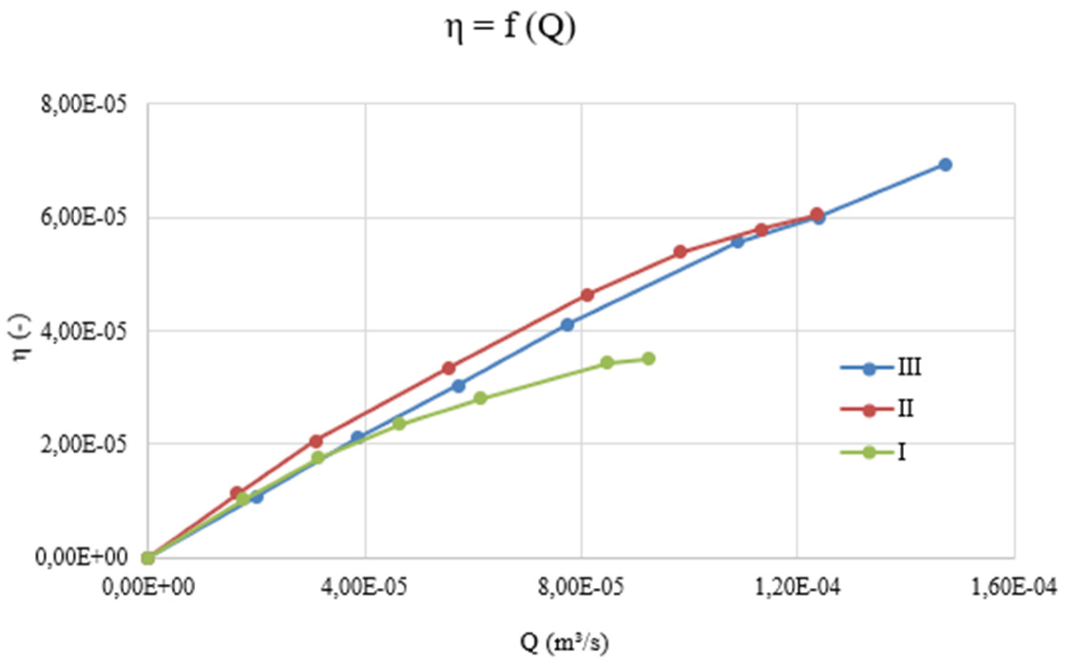

Table 1.
Control valves positions depending on the connection scheme.
| Valve | Connection scheme | |||||
|---|---|---|---|---|---|---|
| TBD | TBU | BTD | BTU | TT | BB | |
| 001 | C | C | O | C | O | C |
| 002 | O | C | C | C | C | O |
| 003 | O | O | C | O | O | C |
| 005 | C | O | O | O | C | O |
| 006 | C | O | C | C | C | C |
| 007 | C | C | O | O | C | O |
| 008 | O | O | C | C | O | C |
*TBD – top-bottom (diagonal); TBU – top-bottom (uniliteral); BTD – bottom-top (diagonal); BTU – bottom-top (uniliteral); TT – top-top; BB – bottom-bottom; O – opened; C – closed.
Table 2.
Sensor specification and sampling rates.
| Sensor type | Measured quantity | Range/ Resolution | Sampling rate | Location in system | Interface protocol |
|---|---|---|---|---|---|
| DS18B20 digital sensor | Temperature | -55 to 125 °C, ±0.5 °C | 1 Hz | T1-T7 (inlet, outlet, radiator surface, ambient) | 1-Wire digital |
| Hall-effect flow meter YF-S201 | Volumetric flow rate | 0-30 L/min, ±5% | 1 Hz | Main loop return line | Pulse counting -> cloud-filtered |
| Pressure sensor M-001 | Gauge pressure | 0-400 kPa, ±1% | 1 Hz | Pump inlet | Analog->ADC->cloud |
| Pressure sensor M-002 | Gauge pressure | 0-400 kPa, ±1% | 1 Hz | Pump outlet | Analog->ADC->cloud |
| Heater electrical module | Voltage, current, power, energy | V: ±1%; I: ±1%, P: ±2% | 1 Hz | Heater block (B-001) | Digital (cloud JSON) |
| Pump electrical module | Electrical power | ±2% | 1 Hz | Pump (P-001) | Digital (cloud JSON) |
| Testo 860i thermal camera | Radiator surface temperature field | 256x192px thermal map | 30 fps (visual only) | Radiator frontal surface | Virtual camera stream |
Table 3.
Steady-state experimental matrix (S-series).
| ID | Heater [B-001] | Pump [P-001] | Flow target | Goal | |
|---|---|---|---|---|---|
| # | P | P | H | - | |
| W | W | m | m3/s | ||
| Scheme of connection: top-bottom (diagonal) | |||||
| S1 | 1000 | 67 | 5 | 8.33e-6 | Low , lower convection, laminar-like |
| S2 | 1000 | 67 | 5 | 2.22e-5 | Medium , reference operating point |
| S3 | 1000 | 67 | 5 | 3.33e-5 | High , higher convection |
| S4 | 500 | 67 | 5 | 2.22e-5 | Medium , low , low heat output |
| S5 | 1500 | 67 | 5 | 2.22e-5 | Medium , high (within safety) |
| Scheme of connection: bottom-bottom | |||||
| S6 | 1000 | 67 | 5 | 2.22e-5 | Medium , compare vs S2 |
| S7 | 1000 | 93 | 6 | 2.22e-5 | Medium-high , effect of higher pump speed |
| S8 | 1000 | 45 | 3 | 8.33e-6 | Low , poor distribution |
| Scheme of connection: top-top | |||||
| S9 | 1000 | 67 | 5 | 2.22e-5 | Medium , compare vs S2, S6 |
| S10 | 500 | 67 | 5 | 2.22e-5 | Medium , low-power alternative |
| S11 | 1500 | 67 | 5 | 2.22e-5 | Medium , high-power altertnative |
Table 4.
Extended hydraulic configuration (S-series).
| ID | Scheme of connection | Heater [B-001] | Pump [P-001] | Flow target | Goal | |
|---|---|---|---|---|---|---|
| # | - | P | P | H | - | |
| W | W | m | m3/s | |||
| S12 | top-bottom (uniliteral) | 1000 | 67 | 5 | 2.22e-5 | asymmetry effect |
| S13 | bottom-top (diagonal) | 1000 | 67 | 5 | 2.22e-5 | alternative diagonal |
| S14 | bottop-top (uniliteral) | 1000 | 67 | 5 | 2.22e-5 | worst-case distribution |
Table 5.
Dynamic experimental matrix (D-series).
| ID | Heater change | Pump change | Valve action | Goal |
|---|---|---|---|---|
| # | W | W | - | - |
| D1 | 500→1500 | constant (67) | None | thermal inertia, response |
| D2 | constant (1000) | speed (45→67→93) | None | jump, regime transition |
| D3 | Constant (1000) | constant (67) | Partially closed | flow reduction, drop, rise |
| D4 | 500→1500 | speed (45→67→93) | None | coupled thermal + hydraulic transient |
Table 6.
Validation matrix (V-series).
| ID | Description | Objective | Acceptance criteria | Recorded data |
|---|---|---|---|---|
| # | - | - | - | - |
| V1 | Temperature sensor calibration | Verify accuracy of temperature sensors T1-T7 | within ±0.2-0.5 K | raw temperature logs, calibration offsets, stability notes |
| V2 | Flow meter validation | Validate FM-001 at low/medium/high flow | relative error (recommended) | flow meter readings, manual flow measurements, error calculation |
| V3 | Pump curve validation | Confirm pump performance at speeds 1-3 | curve deviation within acceptable envelope; no cavitation or instability | differential pressure, flow rate, pump electrical power |
| V4 | Heater power validation | Verify heater electrical output at 500, 1000, 1500 W | electrical power within of nominal | electrical power logs, voltage/current, thermal output (optional) |
Table 7.
Individual flow meter validation results (chronometric method).
| Individual measurements | ||||
| Test ID | Pass/Fail | |||
| m3/s | m3/s | % | ||
| V2-low 1 | 8.461e-6 | 8.500e-6 | +0.47 | Pass |
| V2-low 2 | 8.469e-6 | 8.500e-6 | +0.35 | Pass |
| V2-nom 1 | 2.103e-5 | 2.175e-5 | +3.41 | Pass |
| V2-nom 2 | 2.089e-5 | 2.175e-5 | +4.07 | Pass |
| V2-high 1 | 3.193e-5 | 3.300e-5 | +3.36 | Pass |
| V2-high 2 | 3.282e-5 | 3.300e-5 | +0.56 | Pass |
| Mean values | ||||
| Low | 8.467e-6 | 8.500e-6 | +0.39 | Pass |
| Nominal | 2.097e-5 | 2.175e-5 | +3.74 | Pass |
| High | 3.237e-5 | 3.300e-5 | +1.93 | Pass |
Disclaimer/Publisher’s Note: The statements, opinions and data contained in all publications are solely those of the individual author(s) and contributor(s) and not of MDPI and/or the editor(s). MDPI and/or the editor(s) disclaim responsibility for any injury to people or property resulting from any ideas, methods, instructions or products referred to in the content. |
© 2026 by the authors. Licensee MDPI, Basel, Switzerland. This article is an open access article distributed under the terms and conditions of the Creative Commons Attribution (CC BY) license.
Copyright: This open access article is published under a Creative Commons CC BY 4.0 license, which permit the free download, distribution, and reuse, provided that the author and preprint are cited in any reuse.


