

Submitted:
15 July 2026
Posted:
16 July 2026
You are already at the latest version
Abstract
Since the heavy clutter seriously restricts the ability of radar to detect target, it is significant to build the target detector under heavy clutter. For practical situations without the secondary data or prior knowledge of target and clutter, this paper proposes a polarization-space-time detector. First, a general radar model is constructed for multiple pulses, multiple arrays, and multiple polarizations. Based on the theory of ternary hypothesis, the secondary data free (SDF) GLRT detector is proposed, which can maintain the constant false alarm probability (CFAR) in inhomogeneous clutter. Then, this paper proposes a matrix transform operator and an adaptive detection method using sliding window respectively, which do not need to know the steering vector of radar and the noncentral parameter of clutter in advance, so that the SDF-GLRT detector can adapt to different application scenarios. In addition, this paper optimizes the polarization waveform of the radar system by constructing a projection matrix, which can give the closed-form solutions of the optimal polarization and worst polarization, instead of relying on numerical solution. Finally, the performances of SDF-GLRT detector and other three detectors are compared by simulated and real data, which verifies that SDF-GLRT detector in this paper can still maintain superior performance in various clutter environments without secondary data.
Keywords:
polarimetric radar
; target detector
; GLRT
; heavy clutter
1. Introduction
Marine target detection has broad applications in civil and military fields, among which the target detection under heavy clutter is a hot and intractable issue. With the application of polarimetric radar, a large number of polarimetric detectors show good detection performance, but there are two drawbacks: one is that the secondary data or prior knowledge of target and clutter could limit the use of detector; the other is that the time-space-polarization features are not fully utilized, which also limit the performance of detector. Therefore, this paper mainly aims at the heavy inhomogeneous clutter without secondary data, and proposes a detector in time-space-polarization domain. The relevant references are as follows.
When the probability density functions (PDF) of target and clutter were known, and the covariances of target and clutter were also known, Novak et al. [1] proposed an optimal polarimetric detector (OPD) based on the likelihood ratio test (LRT), which could achieve the optimal probability of detection () while maintaining the constant probability of false alarm (). When only the covariances of target and clutter were known, Novak et al. [1] proposed a polarimetric matched filter (PMF) based on the maximum signal-to-clutter ratio (SCR), and then Wang et al. [2] extended the PMF to the inverse Gaussian clutter. Both OPD and PMF assumed that the polarizations of transmission and reception were same, Boerner et al. [3] proposed the optimal polarimetric contrast enhancement (OPCE), which could simultaneously optimize the polarizations of the transmission and reception. Yang et al. [4] incorporated polarization characteristics into OPCE, i.e., generalized OPCE (GOPCE), and then used GOPCE for ship detection [5]. Based on the SCR and clutter covariance, Yin et al. [6] improved the GOPCE using fisher criterion. Yang et al. [7] defined the minimal cluter-to-signal ratio (MCSR) subspace, which could effectively cover OPCE and GOPCE detectors, and Liu [8] further improved the numerical solution of MCSR. If there was only prior knowledge of clutter, Novak et al. [9,10] proposed a polarimetric whitening filter (PWF) based on the standard deviation and mean value of clutter. Although the detection performance was worse than OPD, it was more executable and verified in [11]. With the multilook polarization data, Lopes et al. [12] proposed the multilook PWF (MPWF) for the K-distribution clutter, and Liu et al. [13] proved that the MPWF detector was equivalent to the maximum likelihood (ML) filter. Due to that PWF and MPWF could not perserve the polarization information, Liu et al. [14] proposed extended MPWF (EMPWF). Gao et al. [15] extended PWF to Gaussian mixture model and Wishart mixture model. As for the MPWF, Liu et al. [16] deduced its PDF and detection threshold under various clutter distributions.
Regarding the connection and difference of OPD, PMF, OPCE, PWF and other detectors, Novak et al. [17] and Yang et al. [18] both compared the performance of these detectors. On the basis of PMF and PWF, Novak[19] constructed a two-parameter CFAR detector using SCR and clutter covariance. Combining OPCE, PMF and PWF, Liu et al. [20] proposed an optimal polarimetric detection filter (OPDF) based on the SCR and speckle. On the basis of [6,7], Liu et al. proposed the subspace polarimetric detection optimization filter (SPDOF) [21] and diagonal loading detector (DLD) [22] using the principle of subspace projection. In [23], Liu et al. gave a general framework of polarization detectors based on quadratic optimization, i.e., generalized DLD (GDLD).
For the polarization detectors based on optimization method such as OPD, PMF, OPCE, PWF and GDLD, the detection performance is elegant in polarimetric SAR, but it does not make full use of the temporal and spatial characteristics. In contrast, detectors such as generalized LRT (GLRT) [24] and adaptive matched filter (AMF) [25] can be extended to the polarization-space-time joint domain. Given the K-distribution clutter, Dilsavor et al. [26] constructed a polarimetric GLRT detector, but the form of detection threshold was complex. In the case of multi-scan, Brown et al. [27] proposed an adaptive multi-scan polarization processor detector based on the GLRT principle. On the premise that polarization information was not needed, Park et al. [28] proposed the polarization-space-time (PST) GLRT detector for complex Gaussian clutter. Pastina et al. [29] built a polarimetric Gaussian (PG) GLRT detector for complex Gaussian clutter to improve the of distributed targets. For the complex Gaussian clutter, Pastina et al. [30,31] expanded the number of polarization channels on the basis of PST-GLRT and then optimized the estimation error of clutter covariance. If the clutter belonged to the compound-Gaussian (CG) model, Pastina et al. [32,33] proposed a texture free (TF) GLRT detector, but the polarization dimension was reduced to two-dimension in order to simplify the solution. When the covariance matrix was singular, Maio[34] proposed a polarimetric modified (PM) GLRT detector using QR decomposition. Due to that the texture parameters of four polarization channels were different, Zhang et al. [35] proposed a polarization detector based on logarithmic GLRT. Park et al. [36] proposed a polarimetric discontinuity detector (PDD), which did not need a two-parameter filter to estimate the polarization parameters. Because the form of GLRT was more complex and the AMF detector was a two-step simplified GLRT, Maio et al. [37] proposed a polarimetric AMF (PAMF) detector for the complex Gaussian clutter. Maio et al. [38,39] extended PAMF to the CG clutter, i.e., PAMF-CG. Subsequently, Maio et al. [40,41] replaced GLRT in PAMF-CG detector with Rao and Wald, thus forming PAMF-Rao and PAMF-Wald detectors. Maio et al. [42] analyzed the detector of distributed targets on the basis of [41]. Wang et al. [43] modeled the sea clutter as CG distribution with the inverse Gaussian texture, and then constructed the corresponding PAMF, PAMF-Rao and PAMF-Wald detectors.
The above GLRT and AMF detectors usually needed to utilize the secondary data, which length must be more than twice of tested signal. Park et al. [44] proposed PST localized GLRT detector based on localized processing technology, which could reduce the length of secondary data, and then given the other two localized processors in [45]. Shen et al. [46] utilized the regularization contraction method to reduce the length of secondary data. Similarly, Francesca et al. [47,48] used the autoregressive model to solve the above problem. In view of the limited secondary data, Maio[49] proposed an AMF-Rao detector using adaptive sidelobe blank. Although the above methods could reduce the length of secondary data, it was difficult to obtain the secondary data in advance in many cases. Therefore, Hurtado et al. [50,51] pioneered a GLRT detector without the secondary data or the prior knowledge of target and clutter, which could adapt to the heavy inhomogenerous clutter. Compared with [50,51], this paper proposes the secondary data free (SDF) GLRT detector, which differences are as follows: First, it is not necessary to know the steering vector of radar system and noncentral parameter of clutter in advance, which is more in line with the real case; Second, it is not necessary to assume that the mean value of clutter is 0, which could adapt to the various clutter environments; Thirdly, it is not necessary to solve the optimal polarization waveform by numerical method, but to adaptively optimize the polarization waveform using the projection matrix method; Fourth, it has better constant false alarm rate (CFAR) in the real data. In general, the main innovations of this paper are:
- 1.
- This paper proposes a SDF-GLRT detector in the polarization-space-time joint domain, which can be applied to any radar system with multiple arrays, multiple pulses and multiple polarizations. With the multi-domain characteristics, the SDF-GLRT detector not only greatly improves its detection performance, but also has well versatility.
- 2.
- Based on the ternary hypothesis, the SDF-GLRT detector can preserve the CFAR property in inhomogeneous clutter. In addition, a new matrix transform operator is built to replace the unknown steering vector matrix, which does not need to know the changing parameters of radar system in advance. For the unknown noncentral parameter of clutter, an adaptive detection using sliding window is proposed in this detector. Through the above three key technologies, the SDF-GLRT detector in this paper does not need the secondary data or prior knowledge, and has good detection performance.
- 3.
- Combining the polarization characteristic of the target and clutter, the closed-form solutions of the optimal polarization and worst polarization are given based on the projection matrix method, instead of relying on numerical solution. Therefore, the transmitted and received polarizations can be comprehensively optimized, in order to improve the performance of SDF-GLRT detector.
This paper is organized as follows. Section II builds the radar model in polarization-space-time joint domain; Section III proposes the mathematical model of SDF-GLRT detector; Section IV analyzes the performances of SDF-GLRT detector; Section V performs experiments based on the simulated and real data; Section VI concludes this paper.
2. Mathematical Model
If the electric field vector of the k-th incident wave is and the magnetic field vector is , the electromagnetic wave [52] in Cartesian coordinate can be expressed as
where, is the elevation angle of incident wave, is the azimuth angle, represents the angle information which dimension is , i.e., . is the polarization angle, is the polarization phase difference, and symbolizes the polarization information.
Assuming that the radar has L vector sensors, the spatial position of l-th vector sensor is . The spatial phase factor of the l-th vector sensor for the k-th incident wave is
where is wavelength.
Then, according to Eqs. (1) and (2), the received signal of the k-th incident wave on the l-th vector sensor is
where is the radar waveform of the k-th incident wave.
As for K incident waves, the received signal on the l-th vector sensor is
where is the noise on the l-th vector sensor, which follows the zero-mean complex Gaussian distribution.
If the received signal contains target , clutter , and noise, the received signal on L vector sensors is
where ⊗ is the Kronecker product operator. is the spatial phase matrix, is the noise matrix, is the steering vector matrix, and is the matrix of target plus clutter, i.e.,
In Eq. (5), the radar waveforms of the target and clutter are the same, i.e., , which are subsequently represented by . Assuming that the target and clutter are in the main-lobe of radar, the spatial angles of different incident wave are approximately the same, i.e., , which are subsequently denoted by . In addition, the polarization information can be further written as
where, represents the polarization scattering coefficient of the k-th target or clutter when the transmitted polarization is h and received polarization is v. indicates the polarization of the transmitted signal.
Combining Eqs. (1), (6) and (7), Eq. (5) is converted to
where, represents the polarization scattering coefficient of target, symbolizes the polarization scattering coefficient of clutter which dimension is , i.e., . The steering vector matrix is
For L vector sensors, D pulses and K different transmitted polarizations, the received signal using Eq. (8) is
where , the dimension of the steering vector matrix is , i.e., .
3. SDF-GLRT Detector
For the manmade target in Eq. (10), we assume that the target is a deterministic vector and its value is . The noise belongs to the zero-mean complex Gaussian distribution with the covariance matrix of . The clutter is a CG distribution of inhomogeneous model, i.e.,
where, is the texture component and is the speckle component. The speckle component follows the complex Gaussian distribution with the mean value of and the covariance matrix of , that is, . As for the target detection in the case of high , i.e., in IPIX radar, the is at level and the texture component remains unchanged between adjacent pulses [40,41,53]. Therefore, the distribution of between adjacent pulses can be equivalent to , where and .
In order to avoid the secondary data, the ternary hypothesis is used to build the SDF-GLRT detector, that is, represents only noise; denotes the signal containing only clutter and noise; indicates that the target, clutter, and noise are existed at the same time, i.e.,
where the steering vector matrix between D pulses is unchanged, that is, is written as for simplification. Similarly, the symbol is abbreviated as d in this paper.
Since the derivations of logarithmic PDF under , and conditions are similar, we will focus on the derivation of condition, while the results of and conditions can refer to that of . Under condition, , and its PDF is
where .
According to Eq. (13), the logarithmic PDF of received signal under D pulses is
where represents the trace of matrix, and is
For the unknown parameters and in Eq. (14), the ML method is utilized for estimation as shown in Eq. (16), which detailed derivation is in Appendix A.
where , , and are
Based on Eq. (A8) in Appendix A, is
Referring to the derivation under condition, the logarithmic PDF under condition is
where is
Similarly, the logarithmic PDF under condition is
where is
where, the mean value of is , i.e., , and its estimation is the same as the result in Eq. (16).
Combining Eqs. (18) and (19), the detector form under condition can be obtained based on GLRT, i.e.,
where .
Due to that the monotonicity of and is the same, can be used as the detector under condition. As for the of , it is the sampling mean value of in Eq. (17), and the statistical distribution of is
Similarly, the middle part of is
where, the statistical distribution of is .
Based on Eqs. (23), (24) and (25), the detector meets the following distribution characteristic[54], i.e.,
where refers to the noncentral F distribution with x and y degrees of freedom, the noncentral parameter is
According to Eqs. (23) - (27), the detector form under condition is
where the statistical distribution of is
In conclusion, with the statistical distribution under and conditions in Eqs. (26) and (29), the SDF-GLRT detector is proposed, as shown below:
where, T is
4. Performance Analysis of Detector
4.1. CFAR Property
When the detection threshold is , the and of SDF-GLRT detector can be obtained based on Eq. (30), i.e.,
If the is assumed to be constant, i.e., , the detector has the CFAR property. Then, the corresponding detection threshold can be calculated using Eq. (32), i.e.,
Using Eq. (33), the corresponding detection threshold can be given, so that the SDF-GLRT detector is a CFAR detector. Since the F distribution of noncentral parameter is a very classical statistical distribution, the look-up table method can be utilized to obtain the detection threshold in Eq. (33). Compared with the look-up table method, this paper provides a more practical and concise method to calculate the detection threshold . First, we can directly obtain the scattered point sequence which meets the distribution of , using the function in Matlab. Then, the statistical distribution map of the scattered point sequence can be given based on the function in Matlab. Finally, we just need to calculate the area of the statistical distribution map according to the , that is, the corresponding detection threshold is the abscissa of the area.
4.2. Adaptive Detection
The mathematical model of SDF-GLRT detector is shown in Eq. (31), where the steering vector matrix and the noncentral parameter are unknown. Differented with other detectors, the SDF-GLRT detector in this paper does not need the secondary data or prior knowledge to get and . Therefore, the SDF-GLRT detector has the ability of adaptive detection, which can be directly applied to any real data. Next, we will introduce in detail how the SDF-GLRT detector adaptively processes the steering vector matrix and the noncentral parameter .
4.2.1. The Steering Vector Matrix
Using Eq. (10), is
According to Eqs. (1) and (2), , , and in can be easily obtained. The tough job is how to calculate the waveform in real time. In [50,51], the is given by the transmit signal energy, the antenna gains of transmitting and receiving, target distance, and receiver sensor array. However, in practical application, the above parameters usually change in different scenarios, which greatly increases the difficulty of parameter estimation.
For the unknown steering vector matrix , this paper conducts a new matrix transformation, as shown below:
where, , and the dimension of diagonal matrix is , i.e., . is
Taking Eq. (35) into (31), the SDF-GLRT detector is
After the matrix transformation using Eq. (35), the SDF-GLRT detector in this paper is only related to , but independent of the transmit signal energy, the antenna gains of transmitting and receiving, target distance, and receiver sensor array. When the radar system has only one set of antenna (such as IPIX radar), is shown in Eq. (38), which form is simpler for adaptive detection.
where, refers to different transmission polarization. For full polarization data, the received signal of any transmission polarization can be directly obtained using digital signal processing, so that the SDF detector can be performed adaptively.
4.2.2. Noncentral Parameter
Based on Eqs. (27) and (29), the noncentral parameter is
where is the mean value at or condition.
In Eq. (39), the noncentral parameter contains multiple unknown parameters, i.e., , , and , which makes it difficult to calculate the detection threshold in Eq. (33). The existing literatures usually assume that there is a secondary data containing only homogeneous clutter to estimate clutter parameter. However, the secondary data will not only limit the application of detectors, but also cannot adapt to the inhomogeneous clutter. In contrast, this paper does not need the secondary data for parameter estimation, but only uses the data of adjacent units to quickly estimate the noncentral parameter . The details are as follows.
Substituting Eq. (16) into (39), the estimation of is
Based on Eq. (40), the estimation of the noncentral parameter can be obtained, which is independent of , and . Subsequently, we construct the sliding window method to realize adaptive detection, as shown in Figure 1. The represents the received data of the d-pulse in the n-th unit to be detected, symbolizes the noncentral parameter estimation of the n-th reference unit, denotes the number of protected units, and is the number of reference units. Using the sliding window method in Figure 1, the noncentral parameter at condition of the tested unit can be quickly obtained, so as to calculate the corresponding detection threshold for adaptive detection. The above method does not require the secondary data for parameter estimation, nor does it need to know , , in advance, so that the SDF-GLRT detector in this paper can be widely used in different scenarios.
4.3. Optimum Polarization
According to Eq. (35), different transmission polarizations will affect the steering vector matrix , and then affect the noncentral parameters and under and conditions at the same time, ultimately affecting the detection performance. If change the noncentral parameters and , the will also change under the premise of maintaining the constant . Since it is difficult to give the closed-form solution of with , , and , this paper combines the polarization characteristics of the target and clutter, so as to give the optimal solution of the steering vector matrix. The details are as follows.
First, the model of the SDF-GLRT detector in Eq. (37) is further converted to Eq. (41), which detailed derivation is shown in Appendix B.
where , and are
where, is the projection matrix, i.e., .
With different transmitted polarizations, i.e., different steering vector matrices , the SDF-GLRT detector under and condition are only related to and as shown in Eq. (41). Since the covariance matrices under and condition are the same, remains unchanged. To sum up, the SDF-GLRT detector under and condition is only related to . Observing in Eq. (42), in order to increase the detector difference under and condition, must be meet the following optimization function:
where and represent at and condition, respectively.
In order to maximize in Eq. (43), the optimal projection matrix should be the subspace of , i.e.,
where, is the projection subspace of , which meets the property of .
Based on Eq. (44), the optimization function of transmitted polarization can be given, i.e.,
Therefore, the optimal transmitted polarization can be obtained based on Eq. (45). Similarly, when the projection matrix is the orthogonal subspace of , as shown in Eq. (46), the SDF-GLRT detector has the worst performance.
where, .
5. Results
In this section, the SDF-GLRT detector proposed in this paper will be verified by combining the simulated and real data. The comparison methods include PST-GLRT detector (refer to Eq. (17) in [28]), TF-GLRT detector (refer to Eq. (12) in [33]) and T-GLRT detector (refer to Eq. (24) in [51]). In addition, the PST-GLRT detector and TF-GLRT detector both need the secondary data for training, but the T-GLRT detector and SDF-GLRT detector do not require any secondary data.
5.1. Simulated Data
Example 1:The and of different detectors under homogeneous clutter with mean value of 0 are analyzed. As for the simulated parameters, the number of pulses D is 10, the number of array antennas L is 4, and the antenna type is crossed dipole, i.e., . The transmitted polarization is divided into two groups, horizontal polarization first and then vertical polarization, i.e., . Assume that the scattering matrix of target is [2.1+1.2j 1.7+1.3j; 1.2+1.9j 2.5+3.1j], i.e., . The number of secondary data of clutter is 80. The is , the clutter-to-noise ratio is 10 , and the scope of SCR is [-10 , 10 ].
The and of the four detectors are shown in Figure 2 and Figure 3. As for the in Figure 2, the results of SDF-GLRT, T-GLRT, and PST-GLRT detector are very close, while that of TF-GLRT detector is slightly higher than the three detectors. From the perspective of which is set as , only the of TF-GLRT detector is higher than the set value and cannot maintain a CFAR property, which is also the reason why its is higher than the other three detectors. In a nutshell, the SDF-GLRT detector proposed in this paper has the same performance as T-GLRT and PST-GLRT detector, and is slightly better than the TF-GLRT detector when the mean value of homogeneous clutter is 0.
Example 2:The experiment is aiming at analyzing the and of different detectors under homogeneous clutter with mean value not being 0. The simulation parameters are consistent withExample 1, only the clutter mean value is set to [1.12+0.96j 0.98+0.70j; 0.74+0.81j 1.78+0.12j].
The and of the four detectors are displayed in Figure 4 and Figure 5. Although the of T-GLRT detector is better than the other three detectors, its is significantly worse than the other three detectors, so that the T-GLRT detector can not be used normally when the mean value is not 0. On the premise that the of SDF-GLRT, TF-GLRT and PST-GLRT detectors are close, the of SDF-GLRT and PST-GLRT detectors are better than of TF-GLRT detector.
Example 3:In this experiment, we will analyze the and of different detectors under inhomogeneous clutter with mean value not being 0. The simulation parameters are consistent withExample 2, except that the homogeneous clutter is changed to the inhomogeneous clutter. The clutter is a K-distribution model, and its PDF is
where, is the scale parameter and is the average energy.
Assuming the scale parameter is 50 and the average energy is 3, the and of the four detectors are as shown in Figure 6 and Figure 7. When the clutter is inhomogeneous clutter, the of the T-GLRT detector is the highest, but its has seriously deviated from . Compared with PST-GLRT, TF-GLRT and SDF-GLRT detectors, the of TF-GLRT and SDF-GLRT is approximately similar, which both higher than that of PST-GLRT detector. In terms of , only the SDF-GLRT detector proposed in this paper can maintain the CFAR property, while the of PST-GLRT and TF-GLRT detectors both are higher than . Compared the in Figure 5 and Figure 7, the performance of PST-GLRT detector decreases under the condition that the mean value of inhomogeneous clutter is not 0, while the SDF-GLRT detector is still effective. Combining the and in Examples 1-3, the SDF-GLRT detector proposed in this paper is superior to the other three detectors.
Example 4:This experiment will verify the optimal combination of transmitted polarization. The simulation parameters are consistent withExample 1, except that the transmission polarization mode is different, i.e., horizontal polarization first, then arbitrary polarization. Based on Eqs. (44), (45) and (46), the optimal polarization and the worst polarization can be obtained. In addition, the vertical polarization is added as the control group.
The under three different transmitted polarizations are shown in Figure 8. Based on the projection matrix using Eqs. (44) and (46), the of the optimal polarization is obviously better than that of worst polarization, which can effectively improve the performance of SDF-GLRT detector. Especially when the SCR is 0 , the of the optimal polarization is higher than 0.22 of the worst polarization.
5.2. Real Data
The real data is from the full polarization IPIX radar, which is collected by Canada’s McMaster University on the shore of Lake Ontario [55]. This paper selects two groups of data for verification, and the relevant parameters are shown in Table 1.
In order to compare the detection performance under different sea states, the sea state of the second group is higher and the SCR is lower than that of the first group. The original images of the two groups are shown in Figure 9 and Figure 10.
In addition, taking the data of No. 310 as an example, the Weibull distribution, K distribution, Alpha-Stable distribution and CG-GIG distribution are used to fit the clutter amplitude, and then the complementary cumulative distributed functions (CCDF) under different distributions are shown in Figure 11. From the perspective of fitting accuracy, the K distribution has a high accuracy for the sea clutter, which further verifies the rationality of the clutter distribution hypothesis in Example 3.
Under different sea states, the detection results of the four detectors are shown in Figure 12 and 13. When the sea state is low, as shown in Figure 12, the four detectors can achieve target detection, but the SDF-GLRT detector proposed in this paper can maintain a lower , which is superior to the performances of the other three detectors. When the sea state is high, as shown in Figure 13, the of the four detectors have decreased, and their have also decreased.
On the premise of achieving target detection, the of four detectors under different sea states are shown in Table 2. In contrast, the T-GLRT detector has the highest . What’s more, with the increase of SCR, the of PST-GLRT and TF-GLRT detector both increase and seriously deviate from , so that they do not have the CFAR property. The above conclusions are consistent with the simulation results in Figure 6 and 7. In contrast, only the SDF-GLRT detector proposed in this paper can maintain a good CFAR on the basis of target detection. Compared with the T-GLRT detector which also does not need secondary data, the performance of SDF-GLRT detector is significantly better. In addition, compared with PST-GLRT and TF-GLRT detectors, the SDF-GLRT detector not only maintains a low , but also does not require secondary data, which is the outstanding advantage of SDF-GLRT detector.
6. Conclusions
In order to detect target in heavy clutter, this paper proposed a SDF-GLRT detector without secondary data, which was constructed by polarization-space-time characteristics. Based on the theory of ternary hypothesis, the SDF-GLRT detector could maintain the CFAR property in inhomogeneous clutter. Then, a new matrix transform operator and an adaptive detection method using sliding window were proposed respectively, which did not need to know the steering vector of radar and the noncentral parameter of clutter in advance. By constructing a projection matrix, the SDF-GLRT detector could give the closed-form solutions of the optimal polarization and worst polarization, instead of relying on numerical solution. Finally, comparing the performances of different detectors using simulated and real data, the SDF-GLRT detector in this paper could still maintain superior performance in various clutter environments without secondary data.
Funding
This research was funded by National Natural Science Foundation of China under Grant number 62501631.
Appendix A. The Detailed Derivation of Eq.(16)
Let rewrite the second part in Eq. (14) as follows:
where .
Duo to that , the third part of Eq. (14) is
where, .
Taking Eqs. (A1) and (A2) into (14), is
where, the equal sign is existed only when .
When is fixed, the estimation of in Eq. (A3) can be obtained using the ML method, i.e.,
In Eq. (A3), only and contain . Therefore, we will first bring Eq. (15) into , as shown below:
According to Eq. (A5), is independent of parameter . Similarly, can be converted to
where, .
Then, the derivative of respect to is
where .
If , is the minimum value. According to Eqs. (A3), (A5), (A6) and (A7), is the maximum value when , i.e.,
where, is
Using Eq. (A9), in (A4) can be further written as:
Appendix B. The Detailed Derivation of Eq.(41)
The SDF-GLRT detector in Eq. (37) is
Referring to diagonal matrix in Eq. (35), we construct the diagonal matrix , i.e.,
where, is the diagonal matrix of , is the diagonal matrix of , and they have the following property.
Substituting Eqs. (B2) (B3) into (B1), the detector is
where, , , and are
References
- Novak, L. M.; Sechtin, M. B.; Cardullo, M. J. Studies of target detection algorithms that use polarimetric radar data. IEEE Trans. Aerosp. Electron. Syst. 1989, vol.25(no.2), 150–165. [Google Scholar] [CrossRef]
- Wang, N.; Liu, L.; Hu, C. B. A novel polarimetric CFAR target detection method. 2011 3rd International Asia-Pacific Conference on Synthetic Aperture Radar, Seoul, Korea, Sep, 2011. [Google Scholar]
- Kostinski, A. B.; Boerner, W. M. On the polarimetric contrast optimization. IEEE Trans. Antennas Propag. 2020, vol.35(no.8), 988–991. [Google Scholar]
- Yang, J.; Dong, G. W.; Peng, Y. N. Generalized optimization of polarimetric contrast enhancement. IEEE Geosci. Remote Sens. Lett. 2004, vol.3(no.1), 171–174. [Google Scholar] [CrossRef]
- Yang, J.; Zhang, H. J.; Yamaguchi, Y. GOPCE-based approach to ship detection. IEEE Geosci. Remote Sens. Lett. 2012, vol.9(no.6), 1089–1093. [Google Scholar] [CrossRef]
- Yin, J. J.; Yang, J.; Xie, C. H. An improved generalized optimization of polarimetric contrast enhancement and its application to ship detection. IEICE Trans. Commun. vol.96(no.7), 2005–2013. [CrossRef]
- Yang, D. W.; Du, L.; Liu, H. W. Novel polarimetric contrast enhancement method based on minimal clutter to signal ratio subspace. IEEE Trans. Geosci. Remote Sens. 2019, vol.57(no.11), 8570–8583. [Google Scholar] [CrossRef]
- Liu, T. Comments on novel polarimetric contrast enhancement method based on minimal clutter to signal ratio subspace. IEEE Trans. Geosci. Remote Sens. 2022, vol.60, 566–572. [Google Scholar]
- Novak, L. M.; Burl, M. C. Optimal speckle reduction in polarimetric SAR imagery. IEEE Trans. Aerosp. Electron. Syst. 1990, vol.26(no.2), 293–305. [Google Scholar] [CrossRef]
- Novak, L. M.; Burl, M. C. Optimal speckle reduction in Pol-SAR imagery and its effect on target detection. Proceedings of SPIE 1101, Millimeter Wave and Synthetic Aperture Radar, Orlando, USA, Aug, 1989. [Google Scholar]
- Novak, L. M.; Burl, M. C.; Irving, W. W. Optimal polarimetric processing for enhanced target detection. IEEE Trans. Aerosp. Electron. Syst. 1993, vol.29(no.1), 234–244. [Google Scholar] [CrossRef]
- Lopes, A.; Sery, F. Optimal speckle reduction for the product model in multilook polarimetric SAR imagery and the Wishart distribution. IEEE Trans. Geosci. Remote Sens. 1997, vol.35(no.3), 632–647. [Google Scholar] [CrossRef]
- Liu, G. Q.; Huang, S. J.; Torre, A. The multilook polarimetric whitening filter (MPWF) for intensity speckle reduction in polarimetric SAR images. IEEE Trans. Geosci. Remote Sens. 1998, vol.36(no.3), 1016–1020. [Google Scholar] [CrossRef]
- Liu, G. Q.; Xiong, H.; Huang, S. J. An extension of multi-look polarimetric whitening filter for speckle reduction in polarimetric SAR images. IEEE International Geoscience and Remote Sensing, Seattle, USA, Jul, 1998. [Google Scholar]
- Gao, W.; Yang, F.; Cui, Y. The extended polarimetric whitening filter and its application to target detection in polarimetric synthetic aperture radar images. IEEE Geosci. Remote Sens. Lett. 2016, vol.13(no.3), 419–423. [Google Scholar]
- Liu, T.; Zhang, J. F.; Gao, G. CFAR ship detection in polarimetric synthetic aperture radar images based on whitening filter. IEEE Trans. Geosci. Remote Sens. 2020, vol.58(no.1), 58–81. [Google Scholar] [CrossRef]
- Chaney, R. D.; Burl, M. C.; Novak, L. M. On the performance of polarimetric target detection algorithms. IEEE Aerosp. Electron. Syst. Mag. 1990, vol.11(no.5), 10–15. [Google Scholar] [CrossRef]
- Yang, Y.; Xiao, S. P.; Feng, D. J. Performance analysis of polarimetric radar detectors. 6th International Symposium on Communications, Control and Signal Processing, Athens, Greece, May, 2014. [Google Scholar]
- Novak, L. M. Target detection studies using fully polarimetric data collected by the Lincoln Laboratory MMW SAR. International Conference on Radar, Brighton, UK, Oct, 1992. [Google Scholar]
- Liu, T.; Dias, R. Y. C. L.; Yang, J. Optimal polarimetric detection filter and its statistical tests for a ship detector. IEEE International Geoscience and Remote Sensing Symposium, Yokohama, Japan, Jul, 2019. [Google Scholar]
- Liu, T.; Jiang, Y. N.; Mari, A.; et al. The polarimetric detection optimization filter and its statistical test for ship detection. IEEE Trans. Geosci. Remote Sens. 2022, vol.60, 5202218. [Google Scholar]
- Liu, T.; Yang, Z. Y.; Mari, A. Joint polarimetric subspace detector based on modified linear discriminant analysis. IEEE Trans. Geosci. Remote Sens. 2022, vol.60, 5223519. [Google Scholar]
- Liu, T.; Yang, Z. Y.; Gao, G. A general framework of polarimetric detectors based on quadratic optimization. IEEE Trans. Geosci. Remote Sens. 2022, vol.60, 5237418. [Google Scholar]
- Kelly, E. J. An adaptive detection algorithm. IEEE Trans. Aerosp. Electron. Syst. 1986, vol.22(no.1), 115–127. [Google Scholar] [CrossRef]
- Robey, F. C.; Fuhrmann, D. R.; Kelly, E. J. A CFAR adaptive matched filter detector. IEEE Trans. Aerosp. Electron. Syst. 1992, vol.28(no.1), 208–216. [Google Scholar] [CrossRef]
- Dilsavor, R. L.; Moses, R. L. A polarimetric generalized likelihood ratio detector for scattering centers in K-distributed clutter. Conference Record of the Twenty-Sixth Asilomar Conference on Signals, Systems and Computers, Pacific Grove, USA, Oct, 1992. [Google Scholar]
- Brown, R.; Wang, H. An adaptive multiscan processor for polarimetric radar. Proceedings of 1994 IEEE National Radar Conference, Atlanta, USA, May, 1994. [Google Scholar]
- Park, H. R.; Li, J.; Wang, H. Polarization-space-time domain generalized likelihood ratio detection of radar targets. Signal Process. 1995, vol.41, 153–164. [Google Scholar] [CrossRef]
- Sciotti, M.; Pastina, D.; Lombardo, P. Polarimetric detectors of extended targets for ship detection in SAR images. International Geoscience and Remote Sensing Symposium, Sydney, Australia, Jul, 2001. [Google Scholar]
- Pastina, D.; Lombardo, P.; Pedicini, V. Adaptive polarimetric target detection with coherent radar. Record of the IEEE 2000 International Radar Conference, Alexandria, USA, May, 2000. [Google Scholar]
- Pastina, D.; Lombardo, P.; Bucciarelli, T. Adaptive polarimetric target detection with coherent radar. I. Detection against Gaussian background. IEEE Trans. Aerosp. Electron. Syst. 2001, vol.37(no.4), 1194–1206. [Google Scholar] [CrossRef]
- Lombardo, P.; Pastina, D.; Corsale, E. Polarimetric coherent adaptive detection against compound-Gaussian clutter. In Proceedings of the 1999 IEEE Radar Conference. Radar into the Next Millennium, Waltham, USA, Apr, 1999. [Google Scholar]
- Lombardo, P.; Pastina, D.; Bucciarelli, T. Adaptive polarimetric target detection with coherent radar. II. Detection against non-Gaussian background. IEEE Trans. Aerosp. Electron. Syst. 2001, vol.37(no.4), 1207–1220. [Google Scholar] [CrossRef]
- Maio, A. D. Polarimetric adaptive detection of range-distributed targets. IEEE Trans. Signal Process. 1997, vol.50(no.9), 1618–1621. [Google Scholar]
- Zhang, Y. X.; Shu, Q. Q.; Jiang, T. A GLRT-based polarimetric detector for sea-surface weak target detection. IEEE Geosci. Remote Sens. Lett. 2022, vol.19, 1500705. [Google Scholar]
- Park, H. R.; Kwang, Y. K.; Wang, H. An efficient adaptive polarimetric processor with an embedded CFAR. ETRI J. 2003, vol.25(no.3), 171–178. [Google Scholar] [CrossRef]
- Maio, A. D.; Ricci, G. A polarimetric adaptive matched filter. Signal Process. 2001, vol.81, 2583–2589. [Google Scholar] [CrossRef]
- Maio, A. D.; Alfano, G. A polarimetric adaptive detector in non-Gaussian noise. In Proceedings of the 2002 IEEE Radar Conference, Long Beach, USA, Apr, 2002. [Google Scholar]
- Maio, A. D.; Alfano, G. Polarimetric adaptive detection in non-Gaussian noise. Signal Process. 2003, vol.83, 297–306. [Google Scholar] [CrossRef]
- Alfano, G.; Maio, A. D. Adaptive polarimetric detection in compound-Gaussian clutter. In Proceedings of the 2003 IEEE Radar Conference, Huntsville, USA, May, 2003. [Google Scholar]
- Maio, A. D.; Alfano, G.; Conte, E. Polarization diversity detection in compound-Gaussian clutter. IEEE Trans. Aerosp. Electron. Syst. 2004, vol.40(no.2), 755–765. [Google Scholar] [CrossRef]
- Conte, E.; Maio, A. D.; Alfano, snf G. Statistical analysis of real clutter at different range resolutions. IEEE Trans. Aerosp. Electron. Syst. 2004, vol.40(no.3), 903–918. [Google Scholar] [CrossRef]
- Wang, Z. H.; He, Z. S.; He, Q. Polarimetric target detection in compound gaussian sea clutter with inverse Gaussian texture. IEEE Geosci. Remote Sens. Lett. 2022, vol.19, 4021205. [Google Scholar]
- Park, H. R.; Kwak, Y. G.; Wang, H. Efficient joint polarisation-space-time processor for nonhomogeneous clutter environments. Electron. Lett. 2002, vol.38(no.25), 1–2. [Google Scholar]
- Park, H. R.; Wang, H. Adaptive polarisation-space–time domain radar target detection in inhomogeneous clutter environments. IEE Proceeding Radar Sonar Navig. 2006, vol.153(no.1), 35–43. [Google Scholar] [CrossRef]
- Shen, L.; Liu, Z. W.; Xu, Y. G. Regularized polarimetric target detection in the presence of inhomogeneous and or non-stationary clutter. CIE International Conference on Radar, Guangzhou, China, Oct, 2016. [Google Scholar]
- Colone, F.; Filippini, F. Autoregressive model based polarimetric adaptive detection scheme part I: Theoretical derivation and performance analysis. IEEE Trans. Aerosp. Electron. Syst. 2020, vol.56(no.5), 3762–3778. [Google Scholar] [CrossRef]
- Colone, F.; Filippini, F. Autoregressive model based polarimetric adaptive detection scheme part II: Performance assessment under spectral model mismatch. IEEE Trans. Aerosp. Electron. Syst. 2020, vol.56(no.5), 3779–3795. [Google Scholar] [CrossRef]
- Maio, A. D. Rao test for adaptive detection in Gaussian interference with unknown covariance matrix. IEEE Trans. Signal Process. 2007, vol.55(no.7), 3577–3584. [Google Scholar] [CrossRef]
- Hurtado, M.; Nehorai, A. Polarization diversity for detecting targets in inhomogeneous clutter. International Waveform Diversity and Design Conference, Pisa, Italy, Jan, 2007. [Google Scholar]
- Hurtado, M.; Nehorai, A. Polarization diversity for detecting targets in inhomogeneous clutter. IEEE Trans. Signal Process. 2008, vol.56(no.4), 1349–1361. [Google Scholar] [CrossRef]
- He, Y. M.; Zhang, T.; Zhou, T. Polarization estimation with vector sensor array in the underdetermined case. IEEE Trans. Geosci. Remote Sens. 2022, vol.60, 5120913. [Google Scholar]
- Conte, E.; Bisceglie, M. D.; Galdi, C. A procedure for measuring the coherence length of the sea texture. IEEE Trans. Instrum. Meas. 1997, vol.46(no.4), 836–841. [Google Scholar] [CrossRef]
- Anderson, T. W. An introduction to multivariate statistical analysis: Third edition. In John Wiley and Sons; Hoboken, New Jersey, USA, 2003. [Google Scholar]
- Drosopoulos, A. Description of the OHGR database. Defence Research Establishment, Ottawa, ON, Canada, 1994. Available online: http://soma.mcmaster.ca/ipix/dartmouth/index.html.
Figure 1.
Adaptive detection based on the sliding window method.
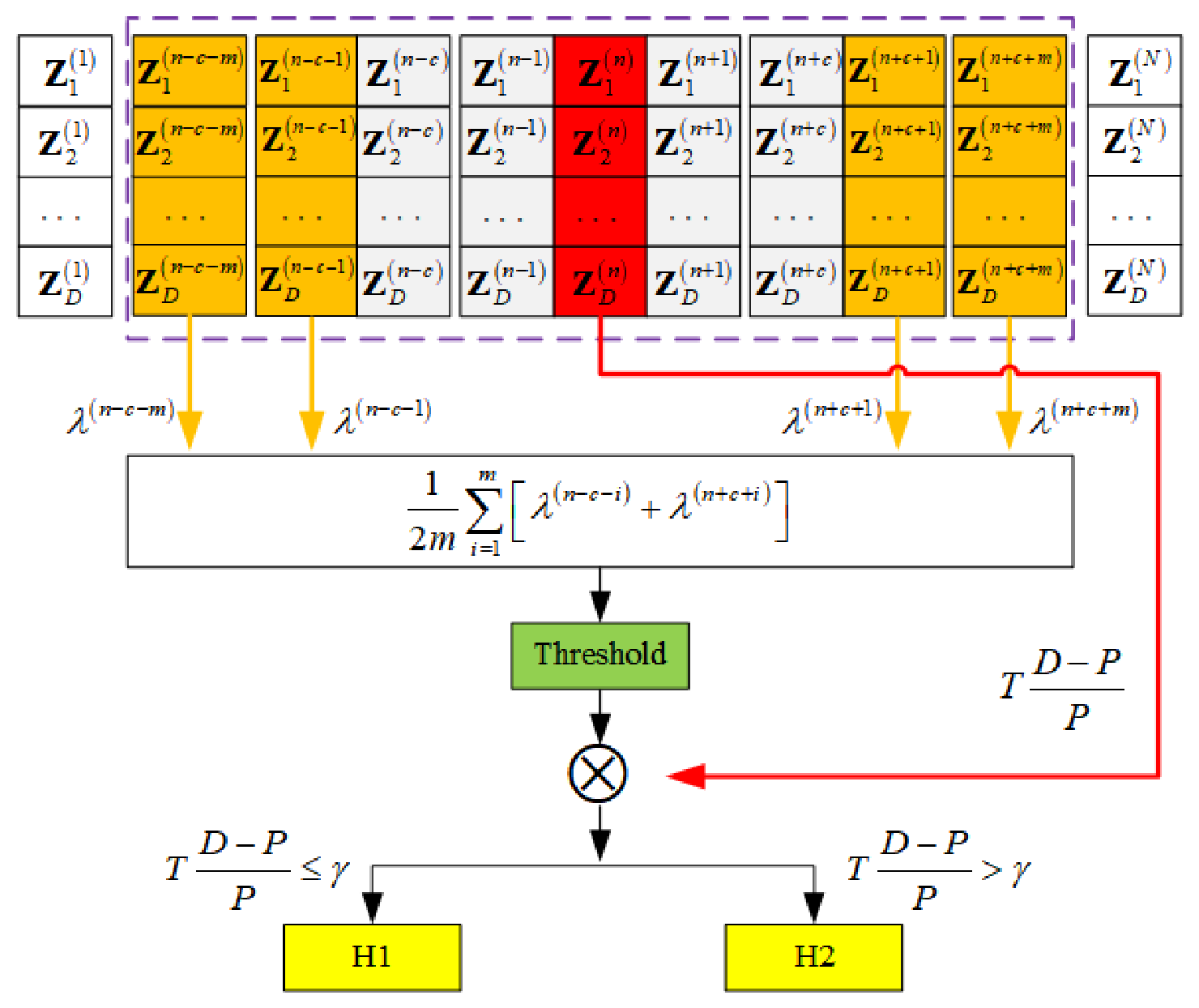
Figure 2.
The under homogeneous clutter with mean value of 0.
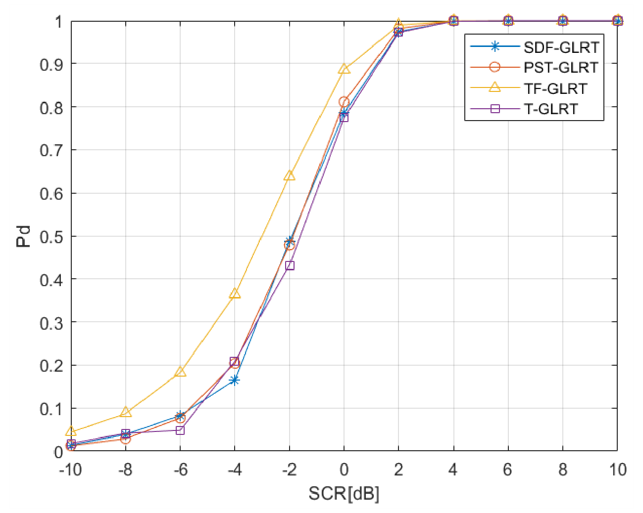
Figure 3.
The under homogeneous clutter with mean value of 0.
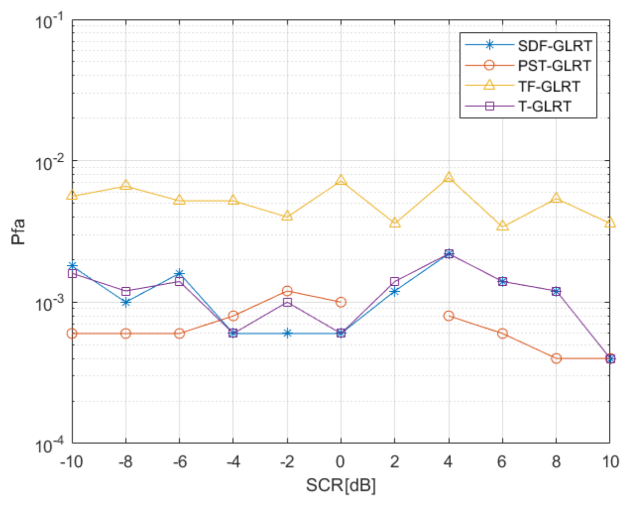
Figure 4.
The under homogeneous clutter with mean value not being 0.
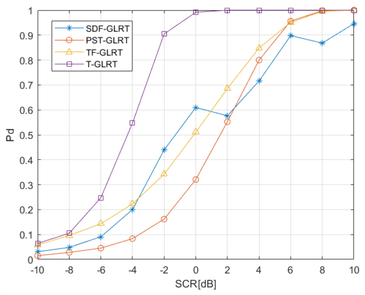
Figure 5.
The under homogeneous clutter with mean value not being 0.
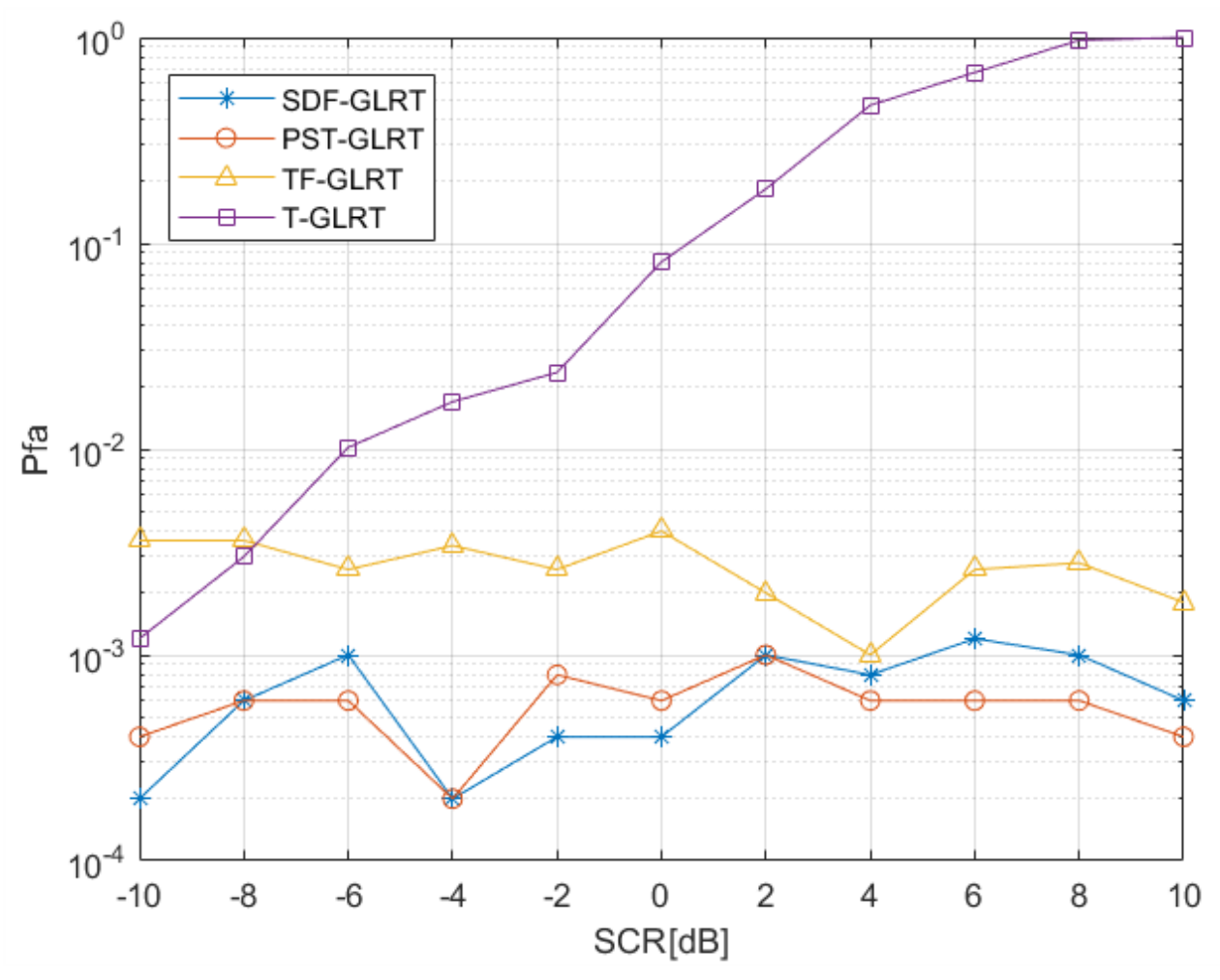
Figure 6.
The under inhomogeneous clutter with mean value not being 0.
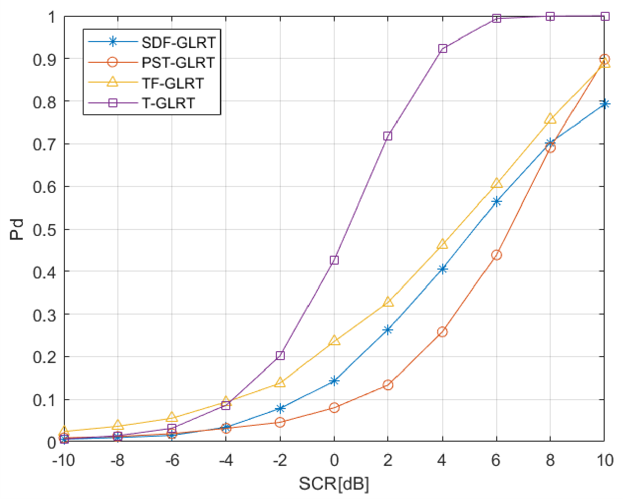
Figure 7.
The under inhomogeneous clutter with mean value not being 0.
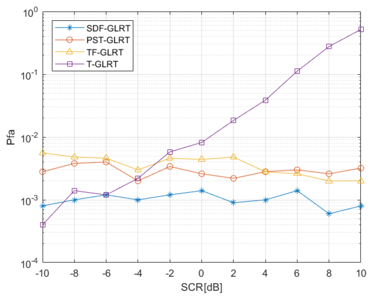
Figure 8.
The of different transmitted polarization.
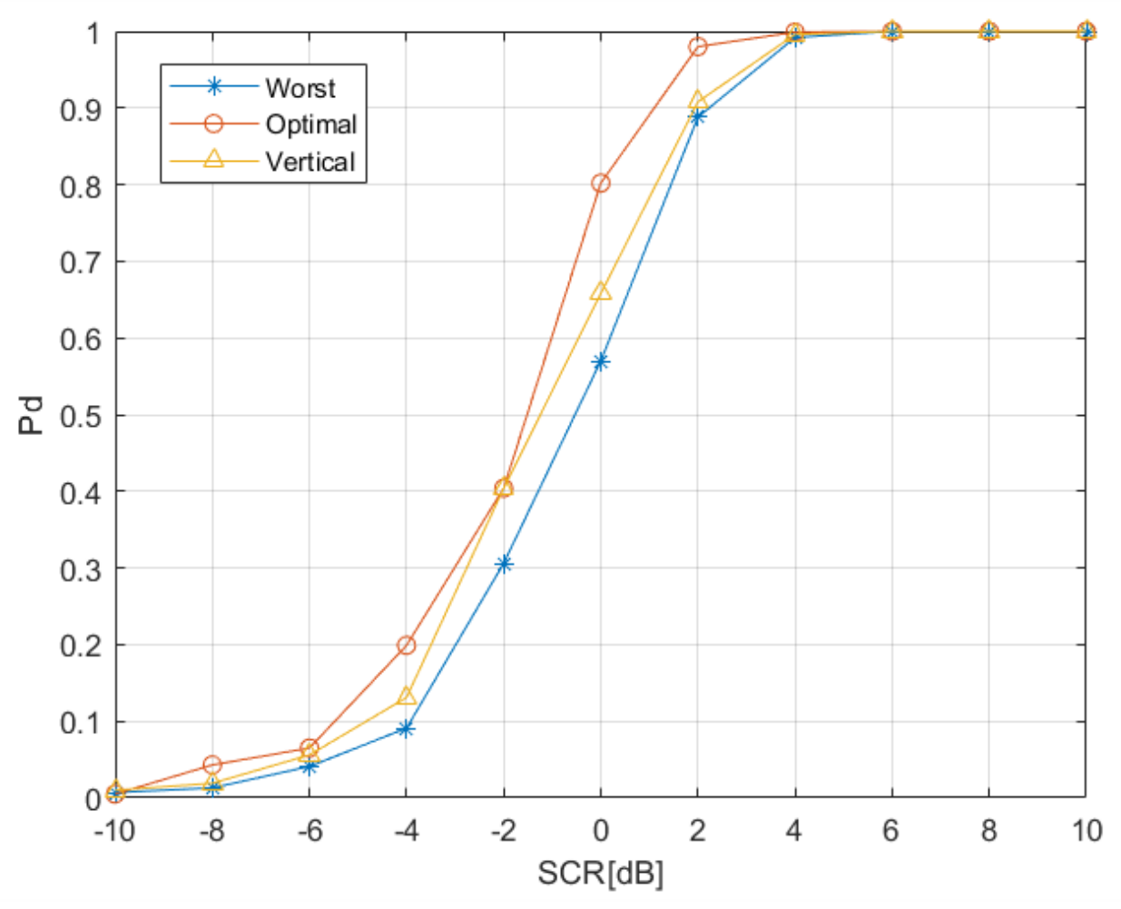
Figure 9.
IPIX radar data of No. 54.
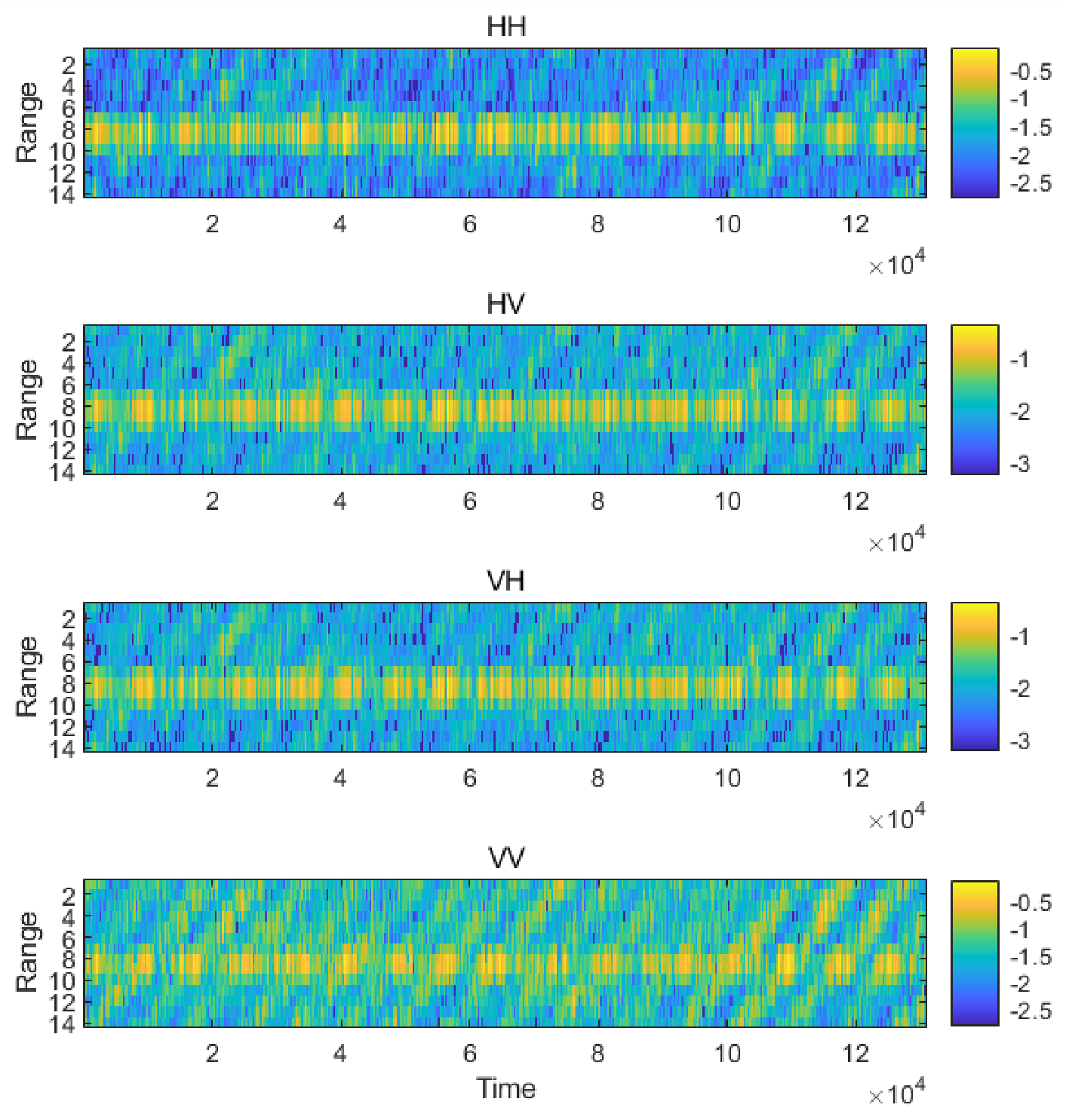
Figure 10.
IPIX radar data of No. 310.
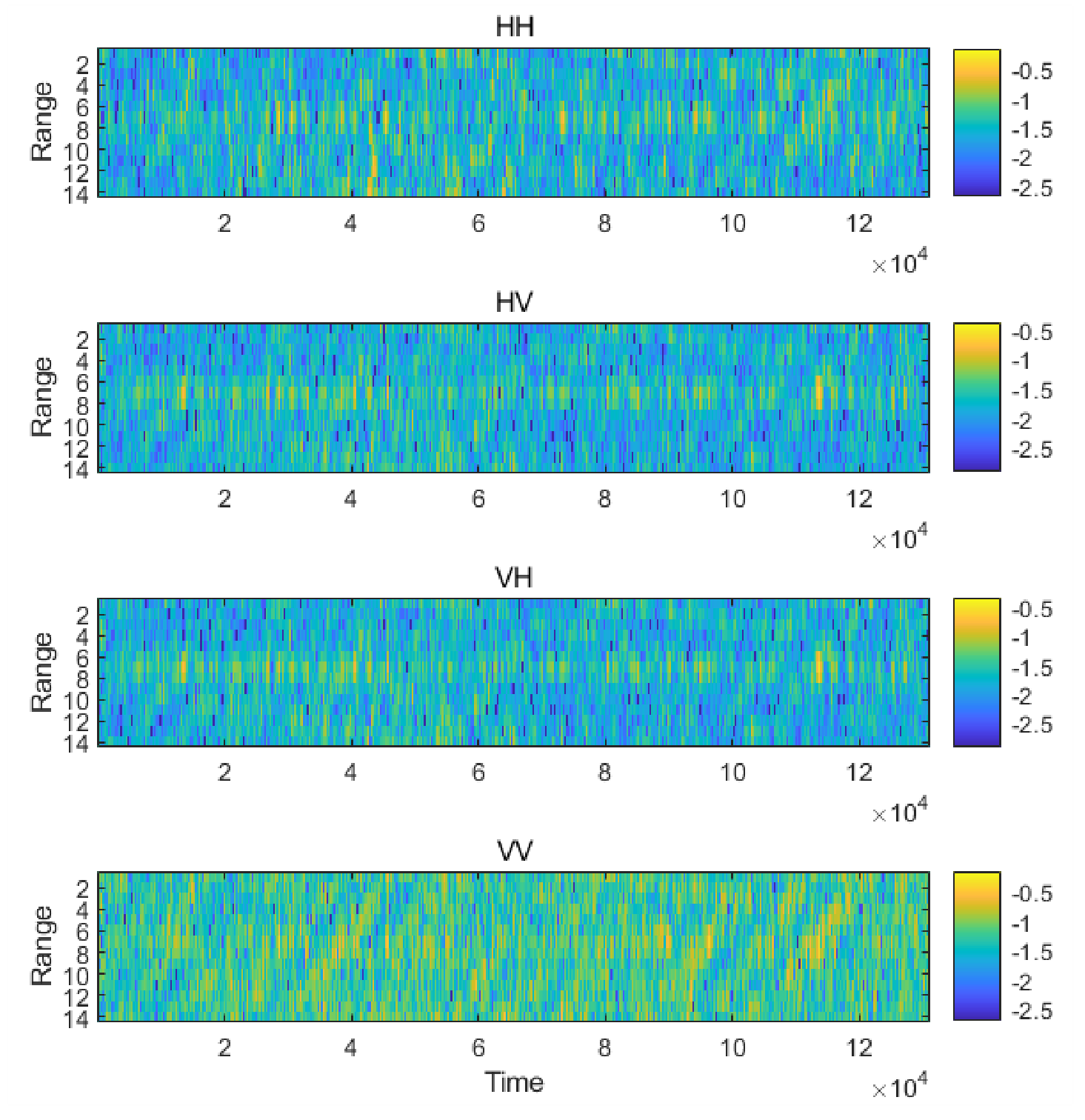
Figure 11.
Fitting results of different clutter distributions.
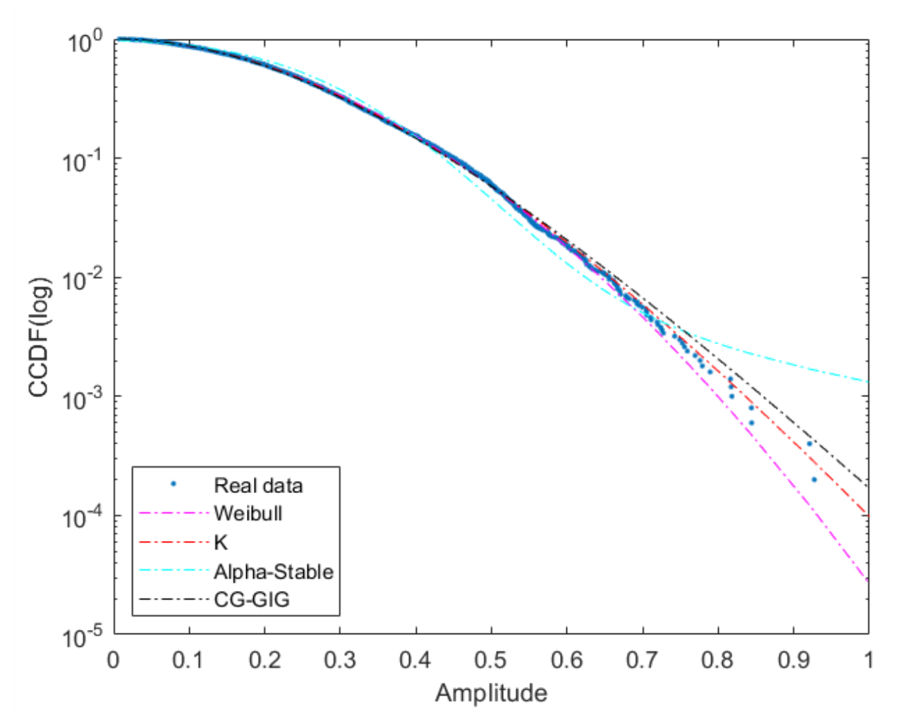
Figure 12.
Detection result of No. 54 data.
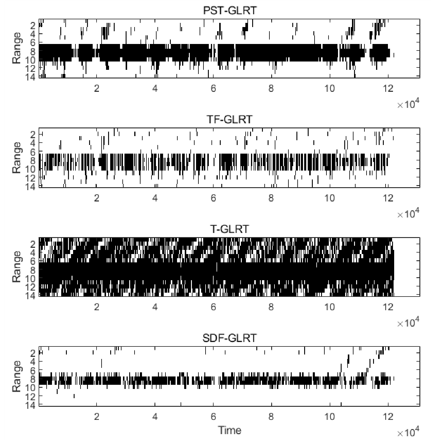
Figure 13.
Detection result of No. 310 data.
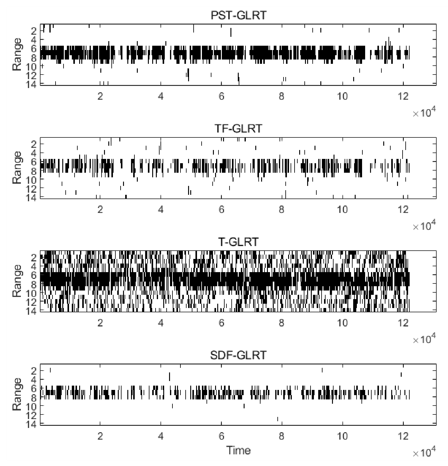

Table 1.
The execution time comparison.
| Data | Time | Number | Wave | Wind | Target Location |
|---|---|---|---|---|---|
| 11.11 | 16:36 | # 54 | 0.7 m | 21 | 8 |
| 11.18 | 16:21 | # 310 | 0.9 m | 33 | 7 |
Table 2.
The of different detectors.
| Data | PST-GLRT | TF-GLRT | T-GLRT | SDF-GLRT |
|---|---|---|---|---|
| 0.0646 | 0.0441 | 0.7405 | 0.0054 | |
| 0.0249 | 0.0242 | 0.3602 | 0.0026 |
Disclaimer/Publisher’s Note: The statements, opinions and data contained in all publications are solely those of the individual author(s) and contributor(s) and not of MDPI and/or the editor(s). MDPI and/or the editor(s) disclaim responsibility for any injury to people or property resulting from any ideas, methods, instructions or products referred to in the content. |
© 2026 by the authors. Licensee MDPI, Basel, Switzerland. This article is an open access article distributed under the terms and conditions of the Creative Commons Attribution (CC BY) license (http://creativecommons.org/licenses/by/4.0/).
Copyright: This open access article is published under a Creative Commons CC BY 4.0 license, which permit the free download, distribution, and reuse, provided that the author and preprint are cited in any reuse.