

Submitted:
16 July 2026
Posted:
16 July 2026
You are already at the latest version
Abstract
Prostate cancer is a primary cause of cancer-related deaths in men which requires its rapid and accurate identification to improve treatment outcomes. This research aimed to develop an innovative, accurate and non-invasive diagnostic framework for the early detection of prostate cancer by combining laser-induced breakdown spectroscopy (LIBS) with machine learning. Prostate cancer and healthy samples were examined using LIBS to analyze their spectra. Elements like calcium, nitrogen and sodium along with the CN-band showed a higher concentration in cancer samples as compared to healthy ones. Various machine learning models were trained to accurately discriminate between cancer and healthy samples. Among several machine learning models, a trilayered neural network achieved the highest training accuracy of 85.0% and the linear SVM model achieved the highest prediction accuracy of 80.0%. Compared to other traditional methods, LIBS emerged as a robust and reliable technique. This study demonstrated the strong potential of combining LIBS with machine learning for the detection of prostate cancer. The technique not only enhanced the diagnostic accuracy but also reduced the need for invasive procedures showing promise for broader medical use.
Keywords:
prostate cancer
; laser-induced breakdown spectroscopy
; elemental analysis
; trilayered neural network
; linear SVM
1. Introduction
Cancer occurs when cells grow uncontrollably and metastasize to other body regions. Prostate cancer is among the most frequently diagnosed cancers among men worldwide. The first instance of prostate cancer by histological analysis was discovered by Adams, a surgeon at The London Hospital in 1853. In 2024 with an expected 299,010 new cases and 35,250 mortality rates, this made prostate cancer (PC) the second most prevalent cancer diagnosed and ranked as the fifth most common cause of cancer-related death among men globally [1]. It is most common in men over the age of 65 or older, less common in the age group of 50 to 64 and rare in men under 50 [2]. The highest estimated rates of prostate cancer are reported in Australia or New Zealand, North America, Western and Northern Europe as well as the Caribbean. In contrast, the lowest rates are from Northern Africa, South-Central Asia, South-Eastern Asia and Eastern Asia. The Caribbean, South Africa and parts of the former Soviet Union have the highest projected mortality rates. In other words, mortality rates are lowest in Asia [3,4]. According to the Lancet commission, several new cases of prostate cancer will rise from 1·4 million in 2020 to 2·9 million by 2040 each year [5]. Prostate cancer diagnosis remains a key challenge in the field of medicine today. The U.S. National Cancer Institute estimates that the annual healthcare costs related to PSA levels detection and treatment of prostate cancer may exceed $275 million [6].
Prostate cancer develops in the prostate gland which is a small walnut-shaped organ situated below the bladder and in front of the rectum. It produces a fluid essential for nourishing and transporting sperm. It occurs when prostate cells begin to grow uncontrollably leading to the formation of abnormal cells. Prostate cancer cells that metastasize to bones or other body parts are called metastatic prostate cancer [7]. Several factors that increase the likelihood of developing prostate cancer include smoking, old age, family history, obesity, alcohol consumption, sexually transmitted infections, high intake of red meat, dairy and saturated fats can lead to an increased risk. A nutrient-dense diet consisting of vegetables, fruits, fish and whole grains offers protective and therapeutic benefits [8]. Regular exercise may also prove beneficial for health [9]. Symptoms include patients may feel difficulty in urinating, frequent urination, weak urinary stream, blood in the urine, chest pain and jaundice. However, backache, pelvis and ribs indicate that the cancer has spread to other parts of the body [10]. The above risk factors indicate the existence of cancer. Aggressive cancer cells spread and become worse and need to be found through prostate-specific antigen (PSA) level testing before it spread all over the body.
Prostate-specific antigen (PSA) is a glycoprotein released by both cancerous and normal cells in the prostate gland. This protein is predominantly found in semen where it plays an important role in liquefying the seminal fluid allowing for the better mobility of sperm. The trace elements of PSA make their way into the bloodstream which is measured during the PSA test. PSA is a basic blood test that measures PSA level in men’s blood. Doctors often utilize it as a primary screening procedure for the early detection of prostate cancer. Over the previous few years, the use of PSA testing has led to a significant improvement in the diagnosis of prostate cancer. It has also led to an understanding of the pathology of pre-cancerous lesions [11]. Recently, various methods have been used for prostate cancer screening and diagnosis, including Raman spectroscopy [12], magnetic resonance imaging [13], computed tomography [14], digital rectal examination [15], PSA testing [16], and biopsy [17]. For treatment, methods such as radiation therapy and hormonal therapy are commonly employed [18]. However, the diagnostic techniques mentioned above still face several challenges including high costs, limited resolution, exposure to discomfort, inadequate sensitivity and overall patient inconvenience [19]. It is important to clarify that infertility and related reproductive concerns are primarily associated with therapeutic interventions rather than diagnostic procedures. Therefore, to minimize patient burden and improve early detection there is a vital need to develop rapid, accurate and reliable diagnostic techniques for the early identification of prostate cancer ultimately helping to reduce mortality rates among men worldwide.
For the analysis of a variety of sample types including solids, liquids and gases, LIBS is a widely used technique that is advanced as well as a systematic analytical technique. The working principle of LIBS includes a highly energetic laser pulse is directed onto the surface of material [20]. LIBS is a reliable method for atomic emission spectroscopy that has gained significant attention in the biomedical sector due to its benefits, including minimal sample preparation, rapid detection and real-time analysis. Numerous studies have utilized LIBS for the detection of various types of diseases. For diabetes, LIBS was used to evaluate sodium and potassium in Ayurvedic anti-diabetic medicine [21] and to investigate the presence of heavy metals linked to the development of colon cancer by analyzing malignant and non-malignant tissue samples using LIBS [22]. In case of kidney stones, LIBS accurately determined the elemental concentrations of sodium, silicon, potassium, iron, magnesium and calcium [23], for identifying microbes causing infectious diseases [24].
Machine learning (ML) is a subset of artificial intelligence where algorithms are trained to analyze huge datasets, make predictions and inform decisions. To identify patterns within data and associate those patterns with specific categories and classes ML surrounds a variety of algorithms designed. ML model can classify individuals as healthy or diseased based on various features. The combination of LIBS and machine learning has shown significant potential in diagnosing various types of cancer like in the case of breast cancer, LIBS-based tissue biopsy analysis has shown high sensitivity in detecting abnormal elemental composition in malignant tissues [25], for the detection of oral cancer LIBS combined with peak area calculation and PCA was applied. It achieved a sensitivity of 95.51% and specificity of 98.64% by measuring intracellular concentrations of potassium and sodium [26], LIBS was applied to identify gastrointestinal stromal tumor tissues and when combined with chemometric-based models such as PLS-DA, k-NN and SVM, it achieved accuracies ranging from 99.44% to 100% [27]. LIBS combined with machine learning was also used for cervical cancer detection. Higher peaks of Na, K, and Mg were found in cancerous tissues while Ca peak was higher in healthy tissues. The chemometric methods of PCA and SVM were combined. They achieved accuracies of 94.44% and 93.06% respectively [28].
PSA elevation correlates with pathological changes in prostate tissue that alter systemic elemental concentrations particularly Ca, Na, N and CN-band. LIBS detects these elemental imbalances, which serves as indirect biomarkers. Therefore, while LIBS is not a replacement for PSA quantification, it provides complementary diagnostic information based on elemental signatures. The novelty in our work is that we did this research on whole blood human samples rather than tissue samples and identified it using LIBS combined with machine learning. Tissue and biopsy samples are significantly more difficult to use in experiments than blood samples because of their complex physical structure, high cellular variation, and strict collection requirements. Blood is a liquid that is easy to standardize, while solid tissue requires destructive processing and introduces many experimental variables. This preliminary research focused on detection of prostate cancer by analyzing elements including Ca, N, Na and CN-band in samples from both prostate cancer patients and healthy individuals. Various machine learning algorithms such as SVM, PCA, k-NN, LDA and DT were applied to classify the samples based on their LIBS spectral data. A trilayered neural network provided the highest training accuracy of 85.0% and the linear SVM model obtained the highest prediction accuracy of 80.0% for the discrimination of both types of samples. This demonstrates that LIBS assisted with machine learning could provide a valuable complementary approach to existing analytical methods for the diagnosis of prostate cancer.
2. Materials and Methods
2.1. Sample Collection and Preparation
The blood samples were taken from the Punjab Institute of Nuclear Medicine (PINUM) Cancer Hospital, Pakistan. Whole blood was selected because it provides a comprehensive elemental profile capturing both cellular and extracellular components that may be affected by prostate cancer. While serum and plasma are more uniform, they exclude information carried within cellular fractions, which may also reflect disease related biochemical changes. Blood sampling is minimally invasive which is why 20 whole blood samples from prostate cancer patients and 20 corresponding samples from healthy donors were taken; all obtained from different individuals in this study. All cancer cases were confirmed as stage III. Each prostate and healthy sample taken from different patients was examined by PINUM Hospital. All the diseased samples belong to stage III, as diagnosed by the pathological department. The Clinical Research Ethics Committee of PINUM Hospital, ensuring compliance with ethical standards, approved the clinical protocol for sample collection. Samples were whole blood withdrawn from a vein of hand vein, pipetted into Ethylenediaminetetraacetic acid (EDTA) tubes to stop clots formation. All samples were kept at 4 °C after their collection and analyzed by the laser-induced breakdown spectroscopy (LIBS) technique within 72 h after collection. Blood samples poured on the boric acid substrate were kept to dry under identical ambient conditions and multiple spectra were collected from different point to average out heterogeneity. Sample Preparation 50 µl of blood was placed on pellets from 99.7% pure boric acid made from 20 MPa pressure in a hydraulic press with a load by 40 mm in diameter. Figure 1 shows the sample preparation process. Each sample had been air-dried for 15 minutes. Laser-ablated spot-by-spot LIBS spectra of 25 spots per sample were acquired by moving the laser focus after each shot to avoid crater-related signal interferences.
2.2. Functionality and Libs Experimental Setup
In this study, a Q-switched Nd: YAG laser (Q-smart 850, Quantel) operating at a repetition rate of 10Hz was used and coupled with a second harmonic of wavelength 532nm with a pulse rate of energy 250 mJ per pulse and a pulse duration of 5 ns. The laser beam of diameter 6mm was precisely focused onto the blood samples using a biconvex lens of a focal length of 10.5 cm to generate laser-induced plasma. Each sample was ablated multiple times to minimize errors due to heterogeneity in blood composition and drying pattern. The emitted plasma light was captured and directed onto an optical fiber connected to a high-resolution spectrometer (AvaSpec 2048–2-USB2, Avantes) which covers a spectral range of 190nm to 770nm with a resolution capability of 0.08nm and it was detected by a charged-couple device (CCD). To synchronize the laser and the spectrometer a delay generator model DG535 from Stanford Research Systems was employed allowed fine adjustment of the trigger timing. The spectrometer trigger was delayed by 1µs to capture the relevant spectral data and the integration time of the CCD was set at 2 ms. A two-dimensional translational stage was incorporated into the setup to precisely position the laser spot on various regions of blood samples. The interference of the surrounding air also leads the fluctuation of spectral signal intensity of samples in the experiment. Therefore, the entire experiment was conducted under standard atmospheric conditions. Figure 2 shows the LIBS experimental setup for the detection of prostate cancer. LIBS generates a high dimensional dataset so machine learning techniques are essential for identifying subtle spectral differences. LIBS spectra were normalized to reduce spectral fluctuations caused by matrix effects and experimental variations thereby improving the reliability of the analysis. Meanwhile, feature lines were selected to serve as inputs for the classifiers, which weakened the influence of fluctuation within the class. The obtained spectra were then processed by using Origin 2021 software to identify the elements present in the sample.
2.3. Data Interpretation and Elemental Analysis
For each 20 cancers and 20 healthy samples, 25 raw spectra were collected. This led to the collection of 500 total raw spectra from the blood samples of cancer patients and 500 total raw spectra from healthy individuals. To reduce changes caused by unpredictable laser energy and different samples, an average was taken after every 5 laser shoots. This approach produced 5 refined spectra per sample across both sample types. As a result, 100 composite spectra of cancer and 100 composite spectra of healthy samples were obtained. The outputs from this process formed the finalized preprocessed spectral dataset. Normalization of every 100 averaged spectra was carried out using the total spectral intensity that is derived from integration across the whole spectral range this process is called normalization and the data is called preprocessed data. The flow chart of the proposed methodology is shown in Figure 3. The process started with blood sample collection, followed by sample preparation and LIBS spectral acquisition. The obtained spectra were preprocessed, and the atomic emission lines of Ca, Na, N, and CN-band were selected as features. These features were then analyzed using the machine learning model to classify the samples as either prostate cancer or healthy.
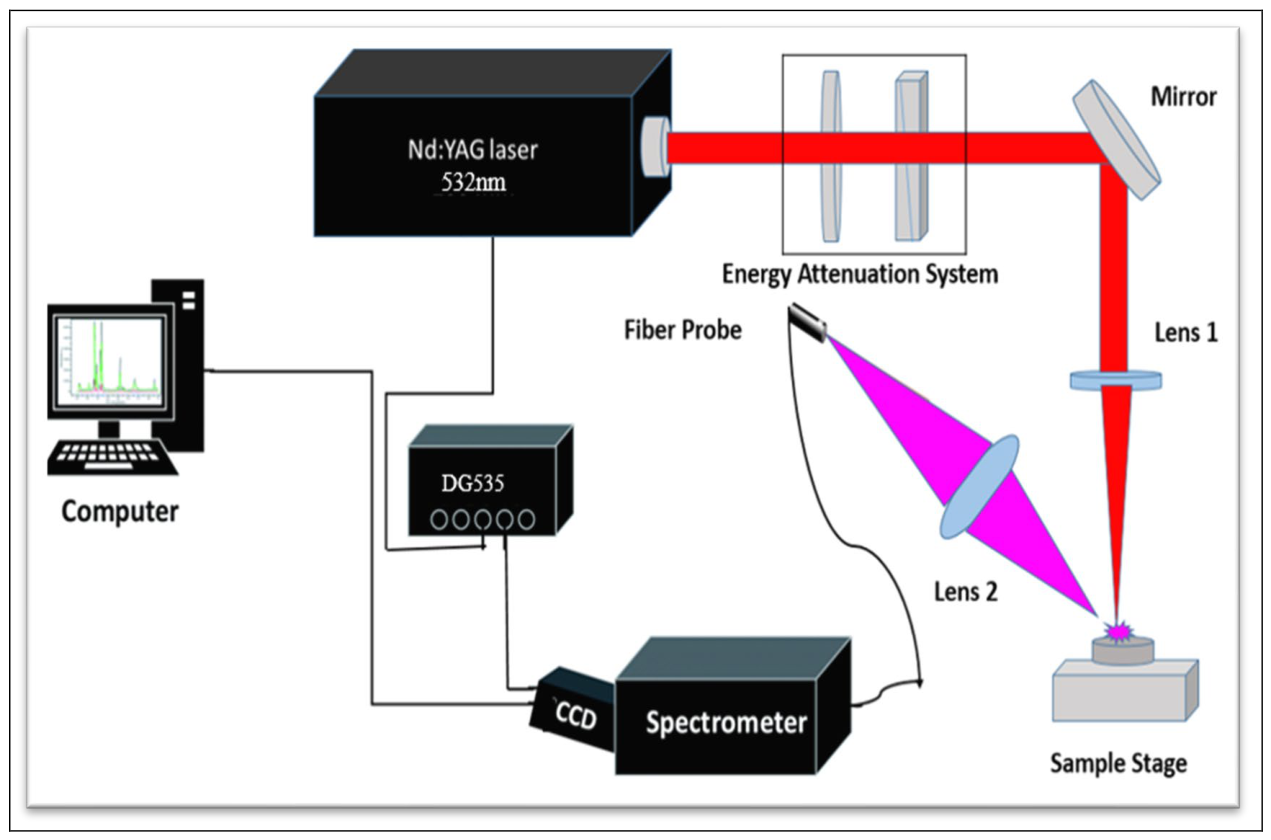
Figure 2.
Schematic of LIBS experimental setup for the analysis of blood samples of prostate cancer.
Figure 2.
Schematic of LIBS experimental setup for the analysis of blood samples of prostate cancer.
In our case, the objective was to compare relative spectral signatures not absolute quantification. Since the same normalization approach was consistently applied across all samples potential artifacts were minimized and class-based differences remained interpretable. Table 1 describes the allocation of samples and spectra for each type of sample.
Elements listed in Table 2 were selected as feature variables for LIBS spectra for further classification. These spectral lines were selected by keeping in mind on their highest intensity in both prostate cancer and healthy samples. The atomic emission lines of Ca, N, Na and the CN-band were seen easily. These atomic emission lines of cancer samples were more vigorous than those of healthy.
When comparing cancer samples to healthy samples, notable differences were observed in LIBS spectra. The substrate used in this work was boric acid. Boric acid was used as a substrate because of its single component and minimal or no interference to blood samples. All samples regardless of clinical status underwent identical preparation ensuring that any matrix effect was uniform across the dataset. It gives a very clean background so the signals from blood samples appear more clearly. It also provides a very smooth and stable surface for the spreading and drying of blood samples ensuring consistent laser interaction. Researchers also used boric acid as a substrate in their research [29]. The spectral lines of Ca, CN-band, N and Na were observed in both types of samples and peaks of B and C were observed from the empty boric acid substrate. In cancer samples the intensities of Ca, CN-band, N and Na increase relative to the healthy samples. Ca plays an important role in regulating cell division which is a process essential for tissue repair, growth and overall cellular health. It is the most common mineral found in human body. It is a primary component of bones and teeth and plays a crucial role in maintaining structural integrity and supporting biochemical processes. Beyond its structural role calcium is plays a vital role in numerous biochemical processes including muscle contraction, blood clotting, hormonal secretion and impulse transmission [30].
Sodium (Na) is a mineral that helps in the absorption of certain nutrients in the intestine. It helps in maintaining the body’s fluid balance, muscle contraction and nerve function. It assists in the active transport of glucose and amino acids across the intestinal lining into the bloodstream [31]. Nitrogen is a fundamental element found in every living cell and plays a central role in growth, repair and metabolic processes. It is a key part of amino acids which are building blocks of proteins. In DNA and RNA nitrogen is also present which carries genetic information and also present in biomolecules like ATP which provides energy for cellular process [32].
CN-band refers to the spectral feature caused by the cyanogen (CN) molecule which is compound consisting of both carbon atom and nitrogen atom. Their biological importance is due to their interaction with oxygen transport and enzyme activity. Figure 3 presents the LIBS spectra of the empty boric acid substrate along with the averaged normalized intensities of various atomic emission lines obtained from both healthy and prostate cancer blood samples. It also includes a combined spectrum that compares the average emission profiles of healthy and cancerous samples allowing for a comparison of spectral differences between the two sample types.
3. Results
3.1. Unsupervised Machine Learning
Principal component analysis (PCA) is an unsupervised machine learning algorithm which widely used in data analysis especially for handling complex data datasets like those from laser-induced breakdown spectroscopy. PCA aims to transform the initial dataset into a new and different set of variables which is known as principal components [33]. In this study, PCA was used on the spectral data matrix for dimensionality reduction and to differentiate between prostate cancer and healthy samples. Figure 4 shows the PCA-based clustering results obtained from both whole blood samples of prostate cancer and healthy individuals. The first three principal components (PCs) in which PC1, PC2 and PC3 together explained most of the variation in the dataset with PC1 alone accounting for 72.63% of the variance, PC2 for 19.49% and PC3 for 4.73%. PCA failed to distinctly classify whole blood samples of prostate cancer and healthy individuals.
3.2. Multivariate Analysis
3.2.1. Supervised Machine Learning
To enhance the ability of LIBS in classification between healthy and prostate cancer samples, machine learning models were applied. From a total of 20 prostate cancer samples, 14 samples with 70 averaged spectra from prostate cancer samples were randomly assigned to the training set while the remaining 6 samples with 30 averaged spectra were used for the prediction set. Similarly, out of 20 healthy samples 14 samples with 70 averaged spectra were randomly selected as training set and the remaining 6 samples with 30 averaged spectra were used for a prediction set. Each sample with their related spectra were selected for the training or prediction set. Therefore, there was no correlation between the spectra of the training and prediction set. The distribution of training and prediction datasets including the number of samples and corresponding spectra for both prostate cancer and healthy whole blood samples presented in Table 3.
In our study, the classification learner app available in MATLAB R2024a was employed to conduct supervised machine learning models on a dataset obtained through LIBS. The PC used for the calculations had an Intel Core i7-6600U processor unit at 2.60 GHz, Windows 10, and 16 GB of RAM. The primary objective was to accurately differentiate between healthy and those diagnosed with prostate cancer, aiming to support rapid detection in medical diagnostics. From the data, 31 models were used to ensure a comprehensive analysis and model comparison. The emission spectra graphs used in this current study were relatively simple compared to more complex biomedical datasets. However, intentionally applied a wide range of machine learning algorithms to evaluate their performance not only for this initial binary classification task for the presence or absence of prostate cancer, but also to identify models with strong generalization capabilities for future work. The long-term objective of this research was to transition from binary classification to a multi-class classification framework which will allow for more detailed preliminary diagnoses of different stages of prostate cancer in future. The current study serves as a foundational step toward that goal. Here, artificial neural network (ANN), support vector machine (SVM), ensemble classifier, decision trees, discriminant analysis, Naive Bayes classifiers and k-NN algorithm were used for the classification between healthy and cancer samples. Further research with large number of samples will provide strong potential of this technique for real-time medical diagnosis in clinical applications.
A decision tree performs its task by building a tree-like structure where each node splits the data based on certain rules. The tree a single root node and each internal node represents a decision node with leaf nodes considered as the final decision or class label. The tree is created by developed by splitting the dataset into many smaller parts called subsets using features that best separate the target classes based on measures like information gain or Gini impurity. If trained on labeled data a well-designed decision tree trained on labeled data can provide high prediction accuracy for classification tasks like disease detection. The quality of the input and the selection of parameters such as the number of splits and maximum depth depend heavily on the performance of the decision tree [34].
Binary logistic regression is a predictive analysis method used when the response or dependent variable is binary in nature like it takes only two possible outcomes healthy vs cancerous. It gives out output as a probability from values between 0 and 1 by taking in a probability function by using the logistic function as the function that estimates the likely output of the classification. It tests the relationship between one or more independent variables with the log odds of the outcome occurring. An essential advantage of the logistic regression is its interpretability, stability and robustness especially when the assumptions such as the absence of linearity in the logit are satisfied [35].
The statistical classification method which is discriminant analysis is a technique to classify two or more classes over the probability distributions. Linear discriminant analysis (LDA) supposes that the predictor variables follows a normal distribution and that all classes have equal variance as well as covariance matrix means that the difference between the classes is primarily due to differences in mean values. This give rise to the linear decision boundaries between the classes. In contrast, quadratic discriminant analysis (QDA) permits each class to have its covariance matrix providing greater flexibility. Rather than linear the resulting decision boundaries are quadratic enabling the model to handle more complex relationships. In both cases the model estimates the probability that a sample belongs to each class and assigns it to the one with the highest probability [36]. A probabilistic algorithm that is Naive Bayes is based on Bayes Theorem that describes the probability of a class given a set of features. The naive assumption is that all features are conditionally independent of each other given the class leading to simplification of computation. The values of continuous features are drawn from a normal distribution it is assumed in Gaussian Naive Bayes. By using kernel functions to estimate the probability distribution offering more flexibility when the feature distributions are not normal Kernel Naive Bayes applies a non-parametric approach at this point. For high-dimensional data Naive Bayes classifiers are especially efficient and require a relatively small amount of test data [37].
In the training dataset a simple non-parametric classification technique which is k-nearest neighbor (k-NN) is use to assign a class to new data point based on its proximity to the “k” nearest data points. Euclidean distance though other metrics such as cosine and Manhattan distance may also be used to calculate the distance between the points. By majority voting among the nearest neighbors the classification decision is made. The class label that appears more frequently among the 5 closest training samples is assigned to the test sample. k-NN is computationally expensive for large datasets but it is also simple to implement [38].
A powerful supervised learning algorithm is designed for classification and regression is the support vector machine (SVM). The primary objective of SVM is to determine the optimal hyperplane that maximally separates data points belonging to different classes. The margin between the closest data points and this hyperplane is maximized to improve generalization. SVM performs well in high-dimensional spaces and maintains strong resistance to overfitting especially in situations even where the number of features exceeds the number of observations. Different kernel functions can be applied to transform the input data into higher dimensions to handle non-linear classifications. A linear kernel is suitable to use when the dataset can be separated using linear line. Quadratic and cubic kernels handle more complex separations [39].
Artificial neural networks (ANN) are machine learning models inspired by the neural architecture of the human brain. They are composed of interconnected layers of nodes where each node processes input and passes it forward through the network. It also consists of an input layer that receives raw features, one or more hidden layers that perform non-linear transformations and an outer layer that provides final classification or prediction. To introduce non-linearity into neural networks and to help the network to learn complex pattern functions like ReLU are used as an activation mechanism. In a single hidden layer narrow neural network contains a small number of neurons. Medium and wide neural networks contain larger hidden layers offering greater representation power. Bilayer and Trilayer neural networks contain multiple hidden layers to record more abstract features [40].
3.2.2. Accuracy Assessment of Predictive Algorithms
A series of classification models were developed and rigorously evaluated using spectral data obtained from whole blood samples to effectively differentiate between the healthy and those diagnosed with prostate cancer. A robust validation strategy was implemented to ensure the reliability and generalizability of the models. Specifically, a 10-fold cross-validation technique was used throughout the training phase. This method consists of partitioning the training dataset into ten equal subsets. Allowing each subset to serve as a test set once, this process was repeated ten times. Thereby minimizing the chances of overfitting and ensuring the well-defined performance of model on unseen data the average performance across all folds provided a more accurate assessment of the model’s predictive capacity. In enhancing classification performance, the process of model optimization played a critical role. The main goal of optimization process was the identification of the combination of parameters that yielded the highest accuracy and consistency across all folds of the cross-validation. The performance of each optimized classification model along with the corresponding function parameters and configurations in comprehensively represented in Table 4.
The below table summarizes the key performance metrics such as accuracy, sensitivity, specificity and the area under the receiver operating characteristic curve (AUC) offering a comparative view of each model’s effectiveness. The model evaluated in this study demonstrated the performance of machine learning when combined with spectral analysis of whole blood to serve as an accurate and non-invasive diagnostic tool for the early diagnosis of prostate cancer. Through careful model training, validation and parameter tuning this research laid a foundation for future development of a clinically useful diagnostic system based on blood biomarkers.
The assessment of several classification algorithms showed differing degrees of efficiency in differentiating blood samples of cancer and healthy ones. Different models had varying training accuracies ranging from 47.1% to 85.0% and prediction accuracy ranging from 46.7% to 80.0%. Due to overfitting and certain amount of data overlap models provided lower accuracies. Evaluating the performance of classification models goes beyond overall accuracy it involves understanding how well the model can distinguish between healthy and cancer samples in the medical field. Specificity and sensitivity are two critical performance metrics used in this regard. The measure of a model’s capability to correctly detect cases that truly have prostate cancer is referred to as true positive rate (TPR) or sensitivity. A higher sensitivity means that the model is effective in reducing false negatives which means only a few actual cancer samples are mistakenly classified as healthy. On the other hand, the ability of a model to correctly identify healthy samples is called as specificity [41]. A model with high specificity successfully reduces false positives ensuring that healthy individuals are not incorrectly flagged as having cancer. To calculate and interpret these metrics a standard method known as a confusion matrix was applied. This matrix is a structured tabular representation that contrasts the model’s predicted classifications against the actual known outcomes. Each row in the matrix corresponds to the instances classified into a predicted class. While each column corresponds to the actual class depending on the convention used. The values that lie along the matrix’s main diagonal indicates the number of correct predictions where the predicted class matches the true class. These include both true positives and true negatives. On the other hand, values that appear outside the diagonal represents misclassifications either false positive where healthy samples are incorrectly predicted as cancerous and cancer samples are wrongly classified as healthy.
3.2.3. Confusion Matrix and ROC Curve Explanation
The model 2.32 which is a trilayered neural network achieved the highest training accuracy of 85.0%. Figure 5 illustrates the confusion matrix for a trilayered neural network model trained on prostate cancer classification data. The matrix represented the capability of the model to accurately classify instances as either healthy or having prostate cancer. The results indicated that the model correctly classified 86.7% of healthy samples which represents its specificity while 13.3% were incorrectly classified as cancer samples. On the other hand, 83.3% of the prostate cancer cases were correctly classified resulting in its sensitivity whereas 16.7% were misclassified as healthy. The model showed overall effective classification results. Further tuning may be required to improve sensitivity of the model without significantly compromising its specificity.
Figure 6 represents the receiver operating characteristics (ROC) curve for the trilayered neural network model. The curve represents the relationship between the true positive rate and the false positive rate and a steeper curve that reaches towards the top-left corner represents better model performance. The area under the curve (AUC) for this model represents an AUC value of 0.8735 for both healthy and prostate cancer samples. This means that the model was highly capable of differentiating healthy and cancer samples. Figure 7 illustrates the confusion matrix for a linear SVM model evaluated on the testing dataset. The model 2.11 which is a linear SVM achieved prediction accuracy of 80.0%. The matrix represents the ability of the model to correctly classify instances as either healthy or having prostate cancer. The results indicated that the model correctly classified 96.7% cancer samples which represents its sensitivity and 63.3% of healthy samples which represents its specificity. However, 36.7% of healthy samples were misclassified as cancer samples and only 3.3% of cancer samples as healthy. This represented that the model was highly sensitive in detecting cancer but less accurate in identifying healthy samples.
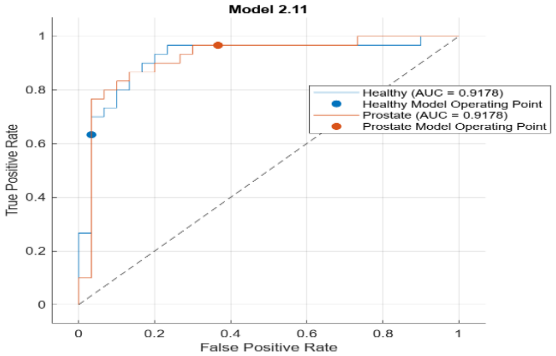
For the linear SVM model, the ROC curve is represented in Figure 8. The area under the curve (AUC) for this model represented an AUC value of 0.9178 for prostate cancer samples and 0.9178 for healthy samples. This means that the model was highly capable of discriminating cancer and healthy samples. The variation in the training and testing accuracy of the ANN is expected with a small dataset and can be overcome by using a large amount of dataset as an input.
Figure 9.
ROC curve of linear SVM evaluated on the testing dataset to discriminate cancer and healthy samples.
Figure 9.
ROC curve of linear SVM evaluated on the testing dataset to discriminate cancer and healthy samples.
4. Discussion
This study demonstrated that LIBS combined with machine learning effectively differentiated prostate cancer and healthy whole blood samples. Prostate cancer disrupts metabolic pathways and systemic homeostasis. This leads to altered mineral regulation particularly in Ca and Na due to inflammation, cell turnover and tumor-associated metabolic activity. These systemic changes are reflected in blood and thus detectable via LIBS. Atomic emission lines of Ca, Na, N, and the CN-band were observed with higher concentrations in cancer samples than in healthy ones. The principal components (PCs) like PC1, PC2 and PC3 together explained most of the variation in the dataset with PC1 alone accounting for 72.63% of the variance, PC2 for 19.49% and PC3 for 4.73%. PCA results of whole blood samples of prostate cancer and healthy individuals didn’t show good results. Several machine learning models including SVM, Ensemble Classifiers, and Neural Networks were evaluated. Among them, the Linear SVM demonstrated the highest testing accuracy (80.0%), while the Trilayer Neural Network achieved the highest training accuracy (85.0%). These results indicate that LIBS combined with machine learning can effectively differentiate prostate cancer and healthy blood samples. As these models has been already used in the identification of other types of diseases. However, we first conduct the test of these machine learning models, and have discussed the relevant results with the clinical doctors of the partner hospitals, and will jointly carry out the detection with other updated models with large number of samples in the future. To a certain extent, the impact of sample differences can be compensated through optimizing and selecting these machine learning models. Previous studies like LIBS combined with machine learning on prostate cancer were examined by using tissue samples. Working in burst mode an Nd: YAG laser with varying time delays for the spectrometer measurements made up the experimental setup. Multiple elemental peaks contributed to observed differences with Fe, Ca and Na. Being more prominent whose concentrations were significantly changed in cancer tissue as compared to healthy ones. At two different time delays of 10µs and 2µs the spectra were recorded. And it was noticed that the spectra were good at 10µs. To enhance classification performance principal component analysis was combined with neural analysis resulting in a high identification accuracy of 97% [42]. Compared to these studies however, we used whole blood samples offered a truly non-invasive and clinically practical approach. Although this introduced greater biological variability, it provided results that were more representative of real-world diagnostic challenges. However, LIBS also had some limitations including sensitivity to sample preparation, biological variability and environmental factors as well as the need for complex data processing to handle high-dimensional spectra. Future developments were suggested to focus on integrating deep learning for improved pattern recognition, creating portable LIBS devices for point-of-care diagnostics, combining LIBS with other spectroscopic methods to enhance diagnostic accuracy and expanding clinical trials for validation. Although the methodological framework employed in this study is similar to our previously reported LIBS-assisted machine learning approach for PCOS detection, the present work introduces a fundamentally different biomedical application. Unlike the PCOS study, which focused on female reproductive disorder screening, the current research investigates prostate cancer using whole blood samples from male patients. The novelty of this work lies in demonstrating that the same LIBS-machine learning framework can successfully identify spectral biomarkers associated with a completely different disease. This highlights the adaptability and broader clinical potential of the proposed methodology for non-invasive cancer diagnostics [43].
5. Conclusions
In this preliminary research, a rapid and efficient approach is introduced for the detection of prostate cancer using LIBS assisted with machine learning. The discrimination analysis was based on 10 atomic emission lines corresponding to four elements Ca, Na, N and CN-band were obtained from both types of samples, either cancer or healthy with higher concentration observed in cancer samples. Although PCA failed to discriminate the types of samples clearly, supervised machine learning significantly improved classification performance. Among the tested models a trilayered neural network achieved the highest training accuracy of 85.0% with a strong specificity of 86.7% and sensitivity of 83.3% while a linear SVM achieved the highest prediction accuracy of 80.0% and excellent sensitivity of 96.7% on the testing set. These results highlighted that different algorithm offer complementary strengths. Neural networks provided balanced classification performance while SVMs excel in detecting cancer cases. Overall, the findings confirm that LIBS coupled with machine learning can be an effective diagnostic approach for distinguishing prostate cancer samples from healthy ones quickly and reliably. With further optimization, larger datasets and clinical validation this technique has strong potential to enhance early screening practices and support decision-making in prostate cancer diagnosis.
Author Contributions
Conceptualization, Fiza Azam, Bushra Sana Idrees, Rabia Nawaz, Yasir Jamil, Shahwal Sabir and Amna Gulzar; Methodology, Fiza Azam, Bushra Sana Idrees, Ayesha Abbas, Shahwal Sabir and Amna Gulzar; Software, Rabia Nawaz, Ayesha Abbas, Shahwal Sabir and Amna Gulzar; Validation, Bushra Sana Idrees, Ejaz Khan, Yasir Jamil, Ayesha Abbas and Shahwal Sabir; Formal analysis, Amna Hameed, Rabia Nawaz and Ayesha Abbas; Investigation, Fiza Azam, Bushra Sana Idrees, Ejaz Khan, Yasir Jamil and Ayesha Abbas; Resources, Fiza Azam and Ejaz Khan; Data curation, Fiza Azam, Bushra Sana Idrees, Ejaz Khan, Rabia Nawaz and Amna Gulzar; Writing—original draft, Fiza Azam and Amna Hameed; Writing—review & editing, Bushra Sana Idrees and Amna Hameed; Visualization, Ejaz Khan and Amna Hameed; Supervision, Bushra Sana Idrees and Yasir Jamil; Project administration, Bushra Sana Idrees and Yasir Jamil; Funding acquisition, Yasir Jamil. All authors have read and agreed to the published version of the manuscript.
Funding
This research received no external funding.
Institutional Review Board Statement
This study was conducted using human blood samples, each obtained from a different patient or volunteer, and analyzed at the Punjab Institute of Nuclear Medicine (PINUM) Cancer Hospital, Pakistan. The clinical protocol was reviewed and approved by the Research Ethics Committee of University of Faisalabad, Pakistan (Reference No. TUF/IRB/459/24) and PINUM Hospital. Individual patient consent was not obtained specifically for this study; however, the PINUM Ethical Committee has an existing agreement with patients that allows the use of their blood samples for future research purposes. The ethics declaration is in accordance with the Declaration of Helsinki.
Data Availability Statement
The original contributions presented in this study are included in the article. Further inquiries can be directed to the corresponding author.
Acknowledgments
All authors are grateful to Prof. Dr. Yasir Jamil for providing access to their laboratory facilities and resources, which made this research possible.
Conflicts of Interest
The authors declare no conflict of interest.
References
- Raychaudhuri, R.; Lin, D.W.; Montgomery, R.B. Prostate cancer: a review. JAMA 2025. [Google Scholar] [CrossRef] [PubMed]
- Rawla, P. Epidemiology of prostate cancer. World J. Oncol. 2019, 10(2), 63. [Google Scholar] [CrossRef] [PubMed]
- Culp, M.B.; Soerjomataram, I.; Efstathiou, J.A.; Bray, F.; Jemal, A. Recent global patterns in prostate cancer incidence and mortality rates. Eur. Urol. 2020, 77(1), 38–52. [Google Scholar] [CrossRef] [PubMed]
- Giona, S. The epidemiology of prostate cancer. In Prostate Cancer; Exon Publications, 2021; pp. 1–15. [Google Scholar]
- James, N.D.; Tannock, I.; N’Dow, J.; Feng, F.; Gillessen, S.; Ali, S.A.; Xie, L.P. The Lancet Commission on prostate cancer: planning for the surge in cases. Lancet 2024, 403(10437), 1683–1722. [Google Scholar] [CrossRef] [PubMed]
- Kim, D.D.; Daly, A.T.; Koethe, B.C.; Fendrick, A.M.; Ollendorf, D.A.; Wong, J.B.; Neumann, P.J. Low-value prostate-specific antigen testing and subsequent health care utilization and spending. JAMA Netw. Open 2022, 5(11), e2243449. [Google Scholar] [CrossRef] [PubMed]
- Habib, A.; Jaffar, G.; Khalid, M.S.; Hussain, Z.; Zainab, S.W.; Ashraf, Z.; Habib, P. Risk factors associated with prostate cancer. J. Drug Deliv. Ther. 2021, 11(2), 188–193. [Google Scholar] [CrossRef]
- Gann, P.H. Risk factors for prostate cancer. Rev. Urol. 2002, 4 (Suppl 5), S3. [Google Scholar] [PubMed]
- Oczkowski, M.; Dziendzikowska, K.; Pasternak-Winiarska, A.; Włodarek, D.; Gromadzka-Ostrowska, J. Dietary factors and prostate cancer development, progression, and reduction. Nutrients 2021, 13(2), 496. [Google Scholar] [CrossRef] [PubMed]
- Gnanapragasam, V.J.; Greenberg, D.; Burnet, N. Urinary symptoms and prostate cancer—misconceptions affecting early presentation and survival. BMC Med. 2022, 20, 264. [Google Scholar] [CrossRef] [PubMed]
- Manji, M. Prostate-specific antigen (PSA): an overview. Ann. Saudi Med. 2002, 22(1–2), 1–3. [Google Scholar] [CrossRef] [PubMed]
- Correia, N.A.; Batista, L.T.; Nascimento, R.J.; Cangussú, M.C.; Crugeira, P.J.; Soares, L.G.; Pinheiro, A.L. Detection of prostate cancer by Raman spectroscopy: a multivariate study. J. Photochem Photobiol. B 2020, 204, 111801. [Google Scholar] [CrossRef] [PubMed]
- Fernandes, M.C.; Yildirim, O.; Woo, S.; Vargas, H.A.; Hricak, H. The role of MRI in prostate cancer: current and future directions. Magn. Reson Mater. Phy 2022, 35(4), 503–521. [Google Scholar] [CrossRef] [PubMed]
- Eissa, A.; Elsherbiny, A.; Coelho, R.F.; Rassweiler, J.; Davis, J.W.; Porpiglia, F.; Bianchi, G. Role of 68Ga-PSMA PET/CT in biochemical recurrence of prostate cancer. Minerva Urol. Nefrol. 2018, 70(5), 462–478. [Google Scholar] [CrossRef] [PubMed]
- Naji, L.; Randhawa, H.; Sohani, Z.; Dennis, B.; Lautenbach, D.; Kavanagh, O.; Profetto, J. Digital rectal examination for prostate cancer screening: a meta-analysis. Ann. Fam. Med. 2018, 16(2), 149–154. [Google Scholar] [CrossRef] [PubMed]
- Tikkinen, K.A.O.; Dahm, P.; Lytvyn, L.; Heen, A.F.; Vernooij, R.W.M.; Siemieniuk, R.A.C.; Agoritsas, T. Prostate cancer screening with PSA test: clinical practice guideline. BMJ 2018, 362, k3581. [Google Scholar] [CrossRef] [PubMed]
- Gravestock, P.; Shaw, M.; Veeratterapillay, R.; Heer, R. Prostate cancer diagnosis: biopsy approaches. In Urologic Cancers; Exon Publications, 2022; pp. 141–168. [Google Scholar] [CrossRef] [PubMed]
- Nomiya, T.; Tsuji, H.; Toyama, S.; Maruyama, K.; Nemoto, K.; Tsujii, H.; Kamada, T. Management of high-risk prostate cancer with radiation and hormonal therapy. Cancer Treat. Rev. 2013, 39(8), 872–878. [Google Scholar] [CrossRef] [PubMed]
- Xiao, J.; Zhang, M.; Wu, D. Side effects of prostate cancer therapies and their management. J. Biol. Methods 2024, 11(3), e99010018. [Google Scholar] [CrossRef] [PubMed]
- Jean-Noel, M.K.; Arthur, K.T.; Jean-Marc, B. LIBS technology and its applications: an overview. J. Env. Sci. Public Health 2020, 4(3), 134–149. [Google Scholar] [CrossRef]
- Kumari, R.; Kumar, R.; Rai, A.; Rai, A.K. Evaluation of Na and K in antidiabetic ayurvedic medicine using LIBS. Lasers Med. Sci. 2022, 37(1), 513–522. [Google Scholar] [CrossRef] [PubMed]
- Gondal, M.A.; Aldakheel, R.K.; Almessiere, M.A.; Nasr, M.M.; Almusairii, J.A.; Gondal, B. Determination of heavy metals in colon tissues using LIBS. J. Pharm. BioMed Anal. 2020, 183, 113153. [Google Scholar] [CrossRef] [PubMed]
- Raheem, S.A.; Habana, S.A.; Ali, A.H. Analysis of kidney stones using single-pulse LIBS. J. Opt. 2024. [Google Scholar] [CrossRef]
- Singh, V.K.; Sharma, J.; Pathak, A.K.; Ghany, C.T.; Gondal, M.A. LIBS for identifying microbes causing infectious diseases. Biophys. Rev. 2018, 10(5), 1221–1239. [Google Scholar] [CrossRef] [PubMed]
- Wei, H.; Zhao, Z.; Lin, Q.; Duan, Y. Elemental distribution in breast cancer tissues using LIBS. Biol. Trace Elem. Res. 2021, 199(5), 1686–1692. [Google Scholar] [CrossRef] [PubMed]
- Winnand, P.; Ooms, M.; Heitzer, M.; Lammert, M.; Holzle, F.; Modabber, A. Real-time detection of bone-invasive oral cancer using LIBS. Oral Oncol. 2023, 138, 106308. [Google Scholar] [CrossRef] [PubMed]
- Idrees, B.S.; Wang, Q.; Khan, M.N.; Teng, G.; Cui, X.; Xiangli, W.; Wei, K. Identification of gastrointestinal stromal tumors using LIBS. BioMed Opt. Express 2022, 13(1), 26–38. [Google Scholar] [CrossRef] [PubMed]
- Wang, J.; Li, L.; Yang, P.; Chen, Y.; Zhu, Y.; Tong, M.; Li, X. Identification of cervical cancer using LIBS and machine learning. Lasers Med. Sci. 2018, 33(6), 1381–1386. [Google Scholar] [CrossRef] [PubMed]
- Chu, Y.; Chen, F.; Sheng, Z.; Zhang, D.; Zhang, S.; Wang, W.; Guo, L. Blood cancer diagnosis using LIBS and ensemble learning. BioMed Opt. Express 2020, 11(8), 4191–4202. [Google Scholar] [CrossRef] [PubMed]
- Tandogan, B.; Ulusu, N.N. Importance of calcium in human health. Turk. J. Med. Sci. 2005, 35(4), 197–201. [Google Scholar]
- Kodintsev, V.V.; Lenda, I.V.; Ponomarev, A.V.; Naumov, N.A.; Salatov, Y.S. Sodium as a vital element in human life. Eur. J. Nat. Hist. 2022, 5, 4–7. [Google Scholar]
- Mullins, B. Nitrogen metabolism and excretion in the human body; 2014. [Google Scholar]
- Zhang, D.; Zhang, H.; Zhao, Y.; Chen, Y.; Ke, C.; Xu, T.; He, Y. Machine learning methods in LIBS data analysis. Appl. Spectrosc. Rev. 2022, 57(2), 89–111. [Google Scholar] [CrossRef]
- Charbuty, B.; Abdulazeez, A. Decision tree-based classification for machine learning. J. Appl. Sci. Technol. Trends 2021, 2(1), 20–28. [Google Scholar] [CrossRef]
- Feng, J.Z.; Wang, Y.; Peng, J.; Sun, M.W.; Zeng, J.; Jiang, H. Logistic regression versus machine learning for survival prediction. J. Crit. Care 2019, 54, 110–116. [Google Scholar] [CrossRef] [PubMed]
- Ha, D.H.; Nguyen, P.T.; Costache, R.; Al-Ansari, N.; Van Phong, T.; Nguyen, H.D.; Pham, B.T. Quadratic discriminant ensemble ML models. Water Resour. Manag 2021, 35(13), 4415–4433. [Google Scholar] [CrossRef]
- Patil, T.R.; Sherekar, S.S. Performance analysis of Naive Bayes and J48 algorithms. Int. J. Comput Sci. Appl. 2013, 6(2), 256–261. [Google Scholar]
- Zhang, Z. Introduction to machine learning: k-nearest neighbors. Ann. Transl. Med. 2016, 4(11), 218. [Google Scholar] [CrossRef] [PubMed]
- Akinnuwesi, B.A.; Olayanju, K.A.; Aribisala, B.S.; Fashoto, S.G.; Mbunge, E.; Okpeku, M.; Owate, P. SVM for early diagnosis of prostate cancer. Data Sci. Manag 2023, 6(1), 1–12. [Google Scholar] [CrossRef]
- Abbasi, A.A.; Hussain, L.; Awan, I.A.; Abbasi, I.; Majid, A.; Nadeem, M.S.A.; Chaudhary, Q.A. Prostate cancer detection using deep learning. Cogn. Neurodyn 2020, 14(4), 523–533. [Google Scholar] [CrossRef] [PubMed]
- Idrees, B.S.; Teng, G.; Israr, A.; Zaib, H.; Jamil, Y.; Bilal, M.; Wang, Q. LIBS-based comparison of blood and serum samples. BioMed Opt. Express 2023, 14(6), 2492–2509. [Google Scholar] [CrossRef] [PubMed]
- Ponce, A.; Flores, T.; Ponce, L. Fast detection of malignant prostate tissue using multipulsed LIBS. Rev. Cuba. Fis. 2022, 39(2). [Google Scholar]
- Nawaz, R.; Idrees, B.S.; Hameed, A.; Azam, F.; Jamil, Y.; Abbas, A.; Sabir, S.; Gulzar, A. Investigation of polycystic ovary syndrome using machine learning-assisted laser-induced breakdown spectroscopy. Opt. Contin. 2026, 5(5), 1663–77. [Google Scholar] [CrossRef]
Figure 1.
The process of sample preparation by depositing blood on boric acid pallet to laser ablation process.
Figure 1.
The process of sample preparation by depositing blood on boric acid pallet to laser ablation process.
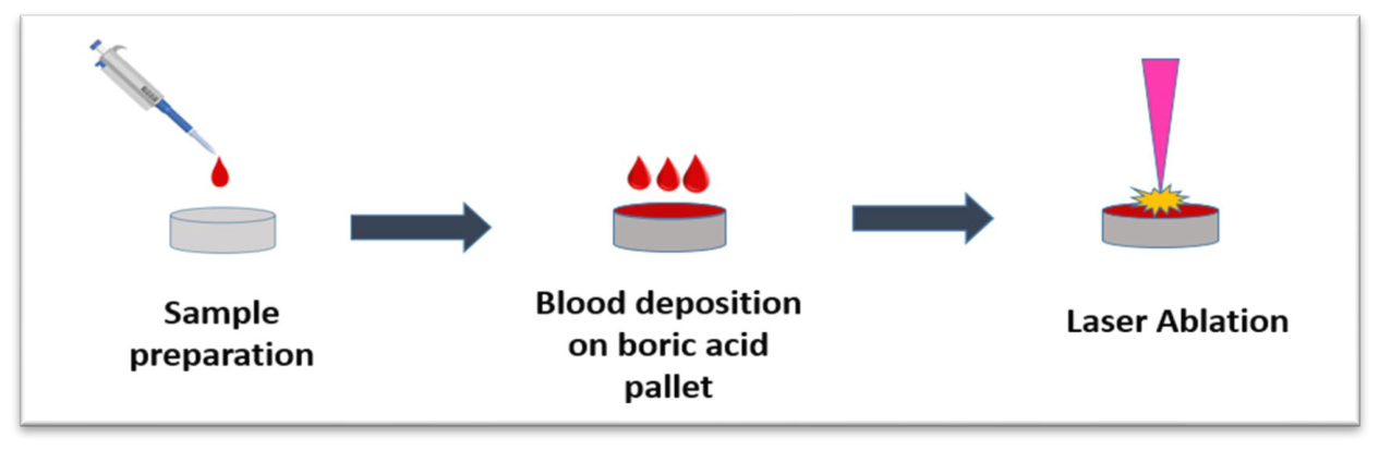
Figure 3.
Flow Chart of data analysis.
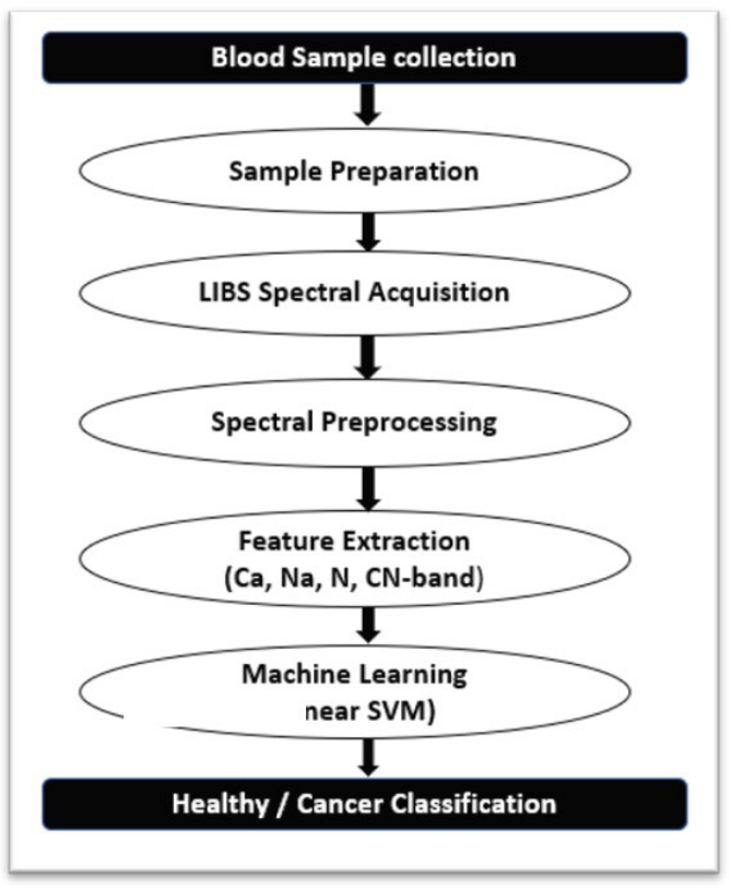
Figure 4.
(a) LIBS spectra representing average normalized intensities of multiple atomic emission lines of healthy samples (b) LIBS spectra representing average normalized intensities of multiple atomic emission lines of prostate cancer samples (c) Combined LIBS spectra representing average normalized intensities of several atomic emission lines of both cancer and healthy samples and (d) LIBS spectra of empty boric acid substrate.
Figure 4.
(a) LIBS spectra representing average normalized intensities of multiple atomic emission lines of healthy samples (b) LIBS spectra representing average normalized intensities of multiple atomic emission lines of prostate cancer samples (c) Combined LIBS spectra representing average normalized intensities of several atomic emission lines of both cancer and healthy samples and (d) LIBS spectra of empty boric acid substrate.
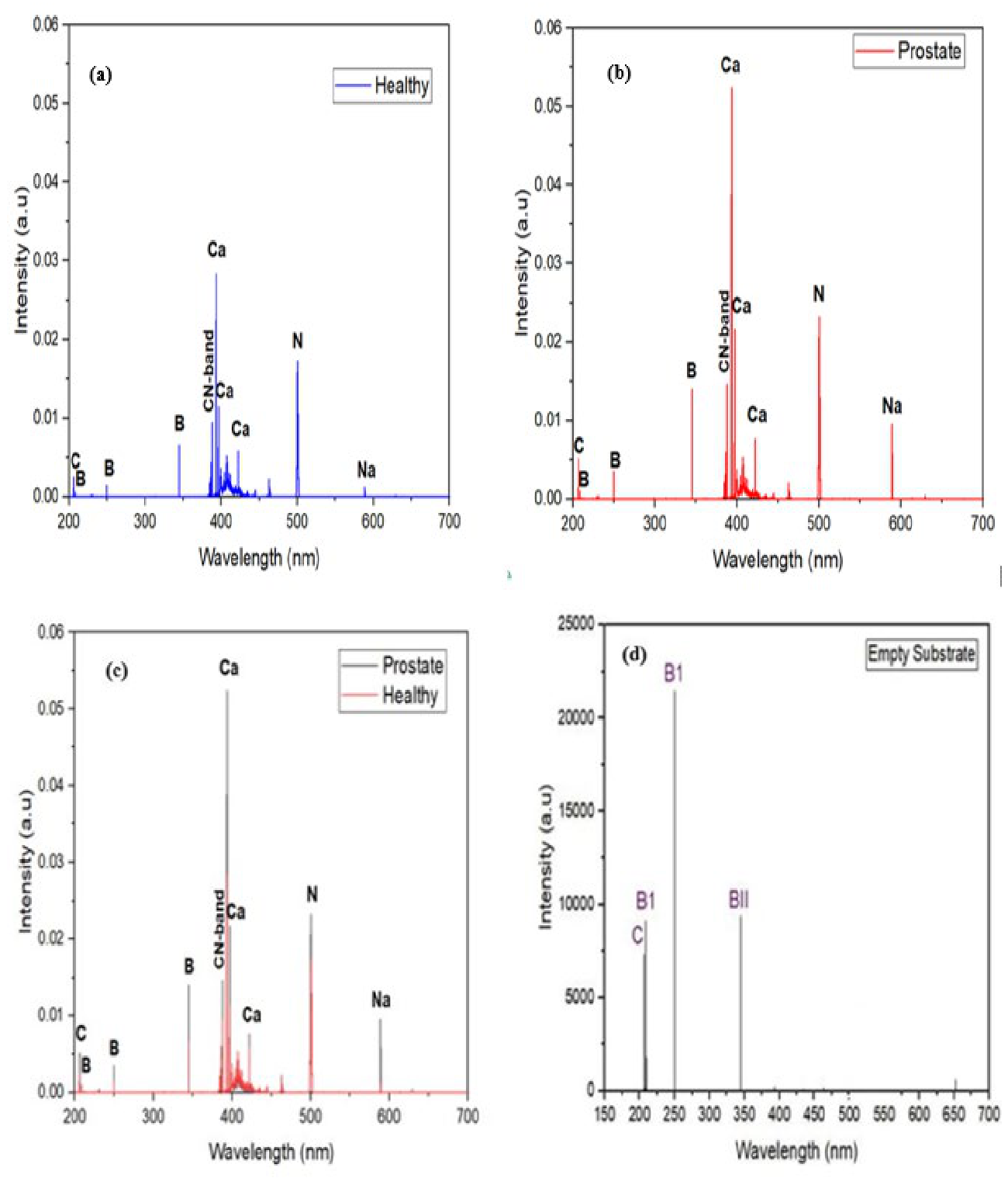
Figure 5.
PCA clustering analysis of whole blood samples of prostate cancer and healthy ones.
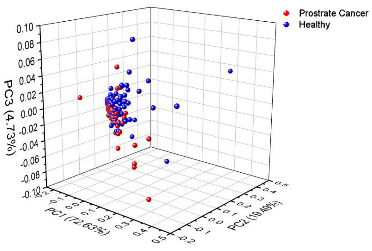
Figure 6.
Confusion matrix of a trilayered neural network evaluated on the training dataset to differentiate between healthy and cancer samples.
Figure 6.
Confusion matrix of a trilayered neural network evaluated on the training dataset to differentiate between healthy and cancer samples.
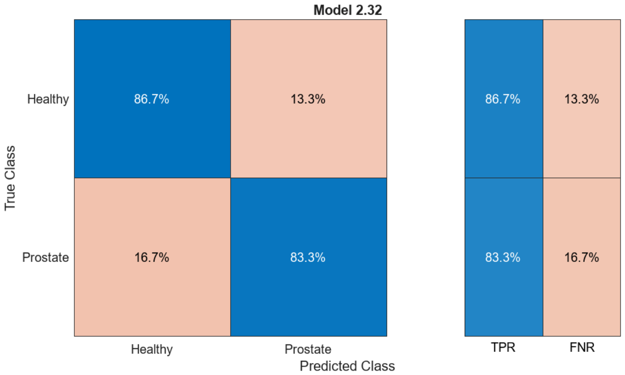
Figure 7.
ROC curve of trilayered neural network evaluated on the training dataset to differentiate between healthy and cancer samples.
Figure 7.
ROC curve of trilayered neural network evaluated on the training dataset to differentiate between healthy and cancer samples.
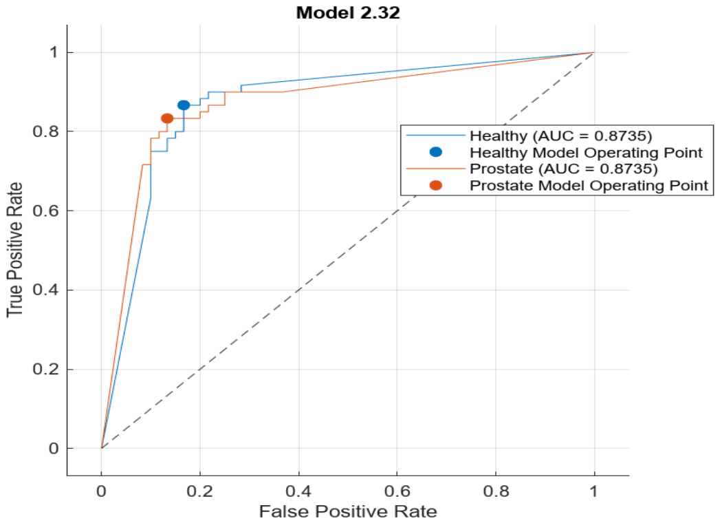
Figure 8.
Confusion matrix of linear SVM interpreted on the testing dataset to discriminate cancer and healthy samples.
Figure 8.
Confusion matrix of linear SVM interpreted on the testing dataset to discriminate cancer and healthy samples.
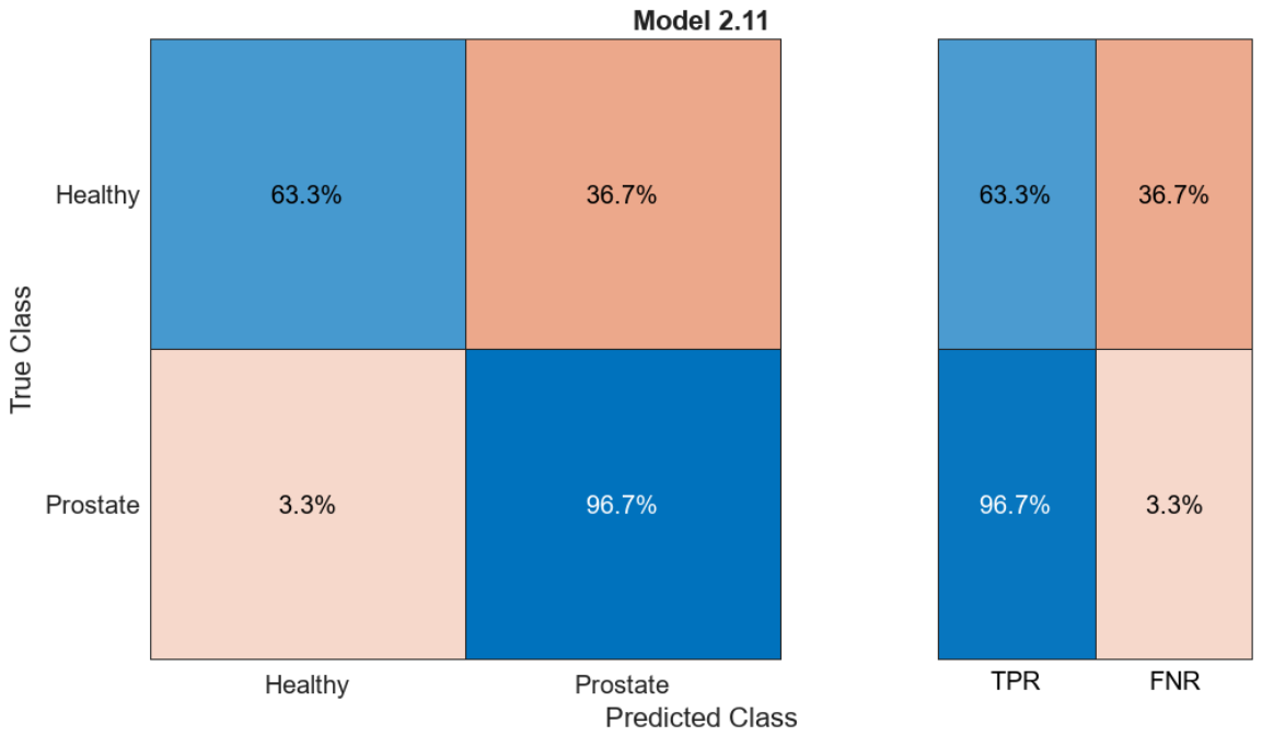

Table 1.
Description of the whole blood samples of both prostate cancer and healthy samples and their spectra.
Table 1.
Description of the whole blood samples of both prostate cancer and healthy samples and their spectra.
| Sample Type | No. of samples | Total no. of raw spectra | Total no. of averaged spectra |
| Healthy | 20 | 500 | 100 |
| Cancer | 20 | 500 | 100 |
Table 2.
Atomic emission lines with corresponding elements.
| Elements | Wavelength (nm) |
| CN-band | 385.7, 386.19, 387.1, 388.3 |
| Ca | 393.4, 396.8, 422.7 |
| N | 500.5 |
| Na | 588.9, 589.5 |
Table 3.
Distribution of training and prediction datasets.
| Data Separation | Samples Information | Cancer | Healthy |
| Training Set | No of samples | 14 | 14 |
| No of spectra | 70 | 70 | |
| Prediction Set | No of samples | 6 | 6 |
| No of spectra | 30 | 30 |
Table 4.
Classification results of various machine learning models for the differentiation of healthy and cancer samples.
Table 4.
Classification results of various machine learning models for the differentiation of healthy and cancer samples.
| Classifier | Classifier Type | Functions | Training Accuracy (%) | Testing Accuracy (%) |
| Binary GLM Logistic Regression |
Regression |
Linear |
72.3 |
60 |
| Efficient Logistic Regression | 70.0 | 59.3 | ||
| Efficient Linear SVM | 79.0 | 60 | ||
| Support Vector Machine (SVM) | Linear SVM | Linear | 72.1 | 80.0 |
| Quadratic SVM | Quadratic | 68.6 | 46.7 | |
| Cubic SVM | Cubic | 71.4 | 65.0 | |
| Fine Gaussian |
Gaussian |
68.6 | 63.3 | |
| Medium Gaussian | 64.3 | 76.7 | ||
| Coarse Gaussian | 57.9 | 51.7 | ||
| Ensemble Classifier | Boosted Trees | AdaBoost | 61.4 | 68.3 |
| Bagged Trees | Bag | 62.9 | 79 | |
| Subspace Discriminant |
Subspace |
77.1 | 61.7 | |
| Subspace k-NN | 63.6 | 60.0 | ||
| RUS Boosted Trees | RUS Boost Bag | 65.0 | 60.0 | |
| Neural Network (NN) | Narrow NN |
ReLU |
80.0 | 61.3 |
| Medium NN | 77.5 | 61.3 | ||
| Wide NN | 74.2 | 60.0 | ||
| Bilayer NN | 80.0 | 71.7 | ||
| Trilayer NN | 85.0 | 60.0 |
Disclaimer/Publisher’s Note: The statements, opinions and data contained in all publications are solely those of the individual author(s) and contributor(s) and not of MDPI and/or the editor(s). MDPI and/or the editor(s) disclaim responsibility for any injury to people or property resulting from any ideas, methods, instructions or products referred to in the content. |
© 2026 by the authors. Licensee MDPI, Basel, Switzerland. This article is an open access article distributed under the terms and conditions of the Creative Commons Attribution (CC BY) license (http://creativecommons.org/licenses/by/4.0/).
Copyright: This open access article is published under a Creative Commons CC BY 4.0 license, which permit the free download, distribution, and reuse, provided that the author and preprint are cited in any reuse.


