

Submitted:
10 July 2026
Posted:
16 July 2026
Read the latest preprint version here
Abstract
Abstract: Numerous studies on non-Hermitian physics have remained confined to isolated exceptional points (EPs) and relied on complex parameters to analyze their physical characteristics [1–20]. Because manipulating such complex variables poses significant engineering constraints in real-world applications, recent efforts have focused on shifting the operational framework towards pure real-parameter spaces or continuous regimes [21–23]. To overcome these limitations, a recent study investigated a purely real-parameter passive system, successfully elucidating an L-surface where innumerable loci of EPs cluster together [24]. To demonstrate that this phenomenon is not an accidental occurrence but a generalized physical trait, we applied this framework to a three-degree-of-freedom semi-definite damped system, thereby establishing its systemic universality. Importantly, we discovered that the inertia of this bare primary mass acts as a critical topological switch: varying its scale governs whether the system coalesces into the L-surface or branches into alternative physical regimes. By treating this ungrounded mass as a key scaling parameter, we define the exact boundaries that map these diverse topological states. Given its high configurability, this framework opens up new avenues for multi-functional wave guiding, adaptive energy harvesting, and highly sensitive topological sensors, expanding the practical utility of non-Hermitian systems previously explored [24].
Keywords:
exceptional point
; critical damping
; analytical exact solution
; purely real parameter
; passive system
; innumerable loci
; semi-definite 3DOF damped system
Main: In recent decades, non-Hermitian physics has fundamentally reshaped our understanding of open quantum and classical systems, driven largely by the exotic properties of exceptional points (EPs) [25,26,27,28,29,30,31,32,33,34,35,36,37,38,39,40,41,42,43,44,45,46,47]. Traditionally, research has focused on isolated EPs or discrete singularities where eigenvalues and eigenvectors coalesce. However, the continuous topological landscapes formed by these singularities, such as exceptional lines or surfaces, remain unexplored, particularly when constrained to purely real-parameter spaces.
The first major step towards expanding these continuous manifolds into reality was achieved by utilizing a purely real-parameter passive system, which unveiled the existence of an L-surface where infinite loci of EPs seamlessly coalesce [24]. However, because this foundational work was tied to a highly specific physical boundary, it remained unclear whether the L-surface was merely a mathematical artifact of that particular setup or a robust, universal phenomenon.
To bridge this gap, we herein transition the discussion to a discrete mechanical platform: a three-degree-of-freedom (3DOF) semi-definite damped system. This specific choice is mathematically and physically deliberate. In a standard two-degree-of-freedom (2DOF) damped system (fixed-free configuration), the topological map remains bounded by conventional boundary conditions. However, transitioning to a 3DOF semi-definite configuration introduces an ungrounded primary mass with singular inertia that fundamentally alters the underlying topological map. By leaving this primary mass entirely free from external constraints, its scale acts as a sovereign parameter. Varying this mass does not merely perturb the system but causes the continuous L-surface to collapse and transfigure into entirely different geometric configurations, representing a profound topological metamorphosis that can never occur in the fixed-free 2DOF framework.
The linear coupling manifold, originally introduced in previous literature [24] to elucidate the coupling dynamics between the primary and secondary systems, is herein expanded and rigorously redefined to accommodate the specific boundary physics of a 3DOF semi-definite damped system (Figure 1a). The free-vibration dynamics of the 3DOF semi-definite damped system are comprehensively governed by the characteristic equation . Here, represents the characteristic matrix, and the eigenvector is defined as =, where , , and indicate the amplitudes of the primary, secondary, and tertiary systems, respectively. The matrix is defined as follows:
In Eq. (1), is an eigenvalue; and are the damping ratio and natural frequency of the secondary system, respectively; and and are the ratios between primary and secondary masses and between secondary and tertiary masses, respectively. The linear coupling manifolds and can be defined as functions of the constant mass ratios (, ) and damping ratio of the secondary system.
In Eq. (2), the linear coupling manifolds, and , are constitutive coupling equations that mathematically and explicitly define the physical interaction among the masses of the primary, secondary, and tertiary systems. Without these manifolds that explicitly define the constitutive coupling relationships, it is virtually impossible to reduce the system’s dimensionality or characterize the existence of EPs within a purely real-parameter space through analytical exact solutions. Specifically, the stiffness and damping parameters of the tertiary system are deterministically formulated as functions of the secondary system’s parameters, represented as and , respectively (Figure 1a). From these constitutive relations, the tertiary damping ratio is rigorously defined as .
Although the manifolds and can be estimated through numerical approximations, such approximate values fail to capture or elicit the comprehensive topological characteristics and unique properties inherent to the EPs. Even a minor variation in the integer values defined in Eq. (2) causes the EPs to collapse abruptly, underscoring the extreme sensitivity and precise configuration required to sustain these topological singularities.
To rigorously establish the systemic universality of the proposed framework and map its topological transitions, we analyze the asymptotic behavior of the coupling relations under extreme mass-ratio limits. Remarkably, by taking the limit of within the functions and , the redefined manifold mathematically reduces exactly to the linear coupling manifold of the conventional 2DOF damped system [24], validating our model as a generalized upper-bound framework (Figure 1b). Conversely, as , the tertiary damping ratio becomes strictly undefined. This mathematical singularity marks the exact onset where the continuous L-surface loses its structural integrity and undergoes a catastrophic collapse.
Furthermore, the scale of acts as a secondary deterministic lever: taking simplifies the intertwined non-Hermitian landscape, causing the tertiary damping to asymptotically converge to . Finally, under the limit , the system recovers a profound topological symmetry where the damping ratios of the secondary and tertiary regimes perfectly equalize ().
In the - plane of Figure 1(b), the boundary of the topological phase transition defining the domain of the complex degenerate roots is determined by substituting various boundary conditions into the sixth-order characteristic equation of derived from Eq. (1). Crucially, because the proposed architecture is a semi-definite system, the rigid-body mode component, represented by , is naturally eliminated from the characteristic equation. Consequently, in the dimensionless domain , the governing formulation can be elegantly reduced to the following fourth-order polynomial equation:
The coefficients – in Eq. (3) are comprehensively detailed in the Methods section. The boundary that rigorously dictates the global topological phase transition of the semi-definite damped system is governed by an eighth-order polynomial within the parameter space of . Consequently, this polynomial serves as the ultimate mathematical engine that maps the entire non-Hermitian landscape and uncovers the hidden boundary physics of the semi-definite system, formulated as follows:
The explicit polynomial coefficients – in Eq. (4) are comprehensively detailed in the Methods section. Distinct from the topological phase transition boundaries of a fixed-free 2DOF damped system [24], the boundaries derived from Eq. (4) characteristically involve the coexistence of both valid physical roots and extraneous roots. In a high-dimensional parameter space, these extraneous roots emerge purely as mathematical artifacts of the polynomial expansion and possess no physical governance over the actual system dynamics. Consequently, to isolate the true deterministic boundaries and ensure that the topological map remains physically meaningful (Figure 2), these extraneous roots must be rigorously filtered and eliminated. The explicit elimination equation utilized to filter out and completely eradicate these spurious roots is formulated as follows:
The coefficients – and – in Eq. (5) are comprehensively defined in the Methods section, and the resulting topological phase transition boundaries (green curves), constructed exclusively from the valid physical roots after eliminating the extraneous ones, are illustrated in Figure 2.
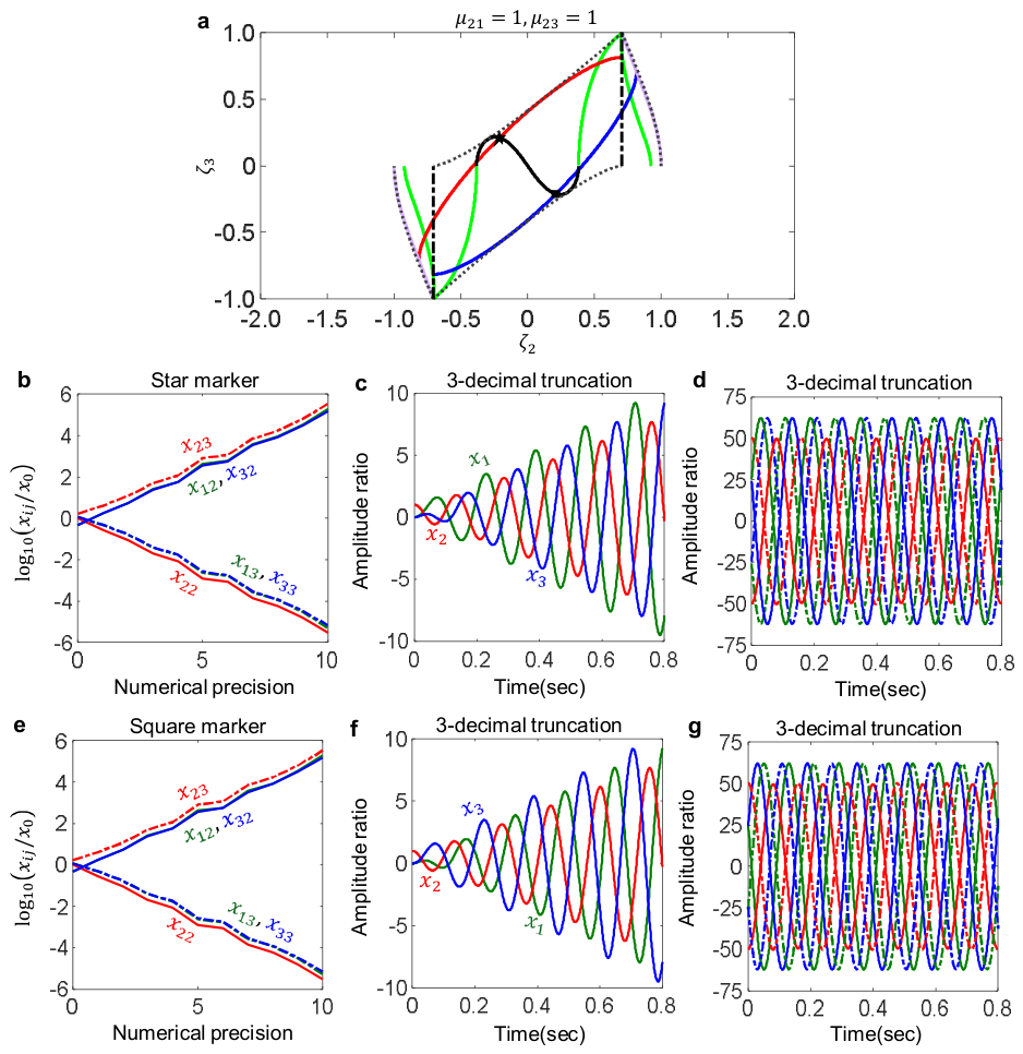
To precisely determine the purely imaginary degenerate roots of Eq. (3), we employ the depressed quartic equation by forcing the cubic coefficient to disappear. Within this continuous framework, these degenerate roots are rigorously defined by the concurrent constraints = 0, = 0, and = 0 (see Supplementary Information (SI)). The resulting continuous points are illustrated by the black curve in Figure 2, which delineates the mathematical nature of the complex double roots according to the following formulation:
Equation (6) yields exactly four analytical roots. To successfully distinguish the valid physical roots among these four candidates, we impose the constraints and ; under this condition, the isolated purely imaginary degenerate roots are determined as follows:
As established in our previous study [24], the loci of exceptional singularities under a constant mass ratio perfectly coincide with the loci of classical critical damping points (CCs). The boundary characterizing the cluster of CCs is rigorously defined as follows:
Consequently, both deterministic loci exhibit complete convergence with an elliptical profile; the continuous elliptic trajectory transitioning seamlessly between both loci can be rigorously defined through the following elliptical equation:
Demonstrating that the continuous trajectory exactly coincides with the two symmetric loci where numerous EPs and CCs cluster in Figure 2. To systematically elucidate the underlying boundary physics, the structural configuration and parameter mapping of the proposed 3DOF semi-definite damped system are schematically illustrated in Figure 1a. Here, the intrinsic parameters of the tertiary system, specifically the stiffness and damping , are rigorously projected onto the functional parameter space (, , and ) of the secondary system. This mathematical bridging is uniquely enabled by the newly expanded linear coupling manifolds and . Through this manifold-based formulation, the boundary effects of the semi-definite system can be comprehensively captured without losing the high-dimensional physical insights of the coupling dynamics.
The rigorous mathematical validity of this projection is topologically demonstrated through the asymptotic limit in Figure 1b. As the primary mass approaches infinity (), the high-dimensional topological map of the semi-definite system uniquely reduces and converges into that of the fixed-free 2DOF system [24]. This exact convergence establishes a definite proof of topological homomorphism, confirming the preservation of topological invariance across different structural dimensions. Consequently, the newly revealed boundary physics serves to encapsulate the classical degenerate states, effectively mapping the broader non-Hermitian landscape without discontinuity.
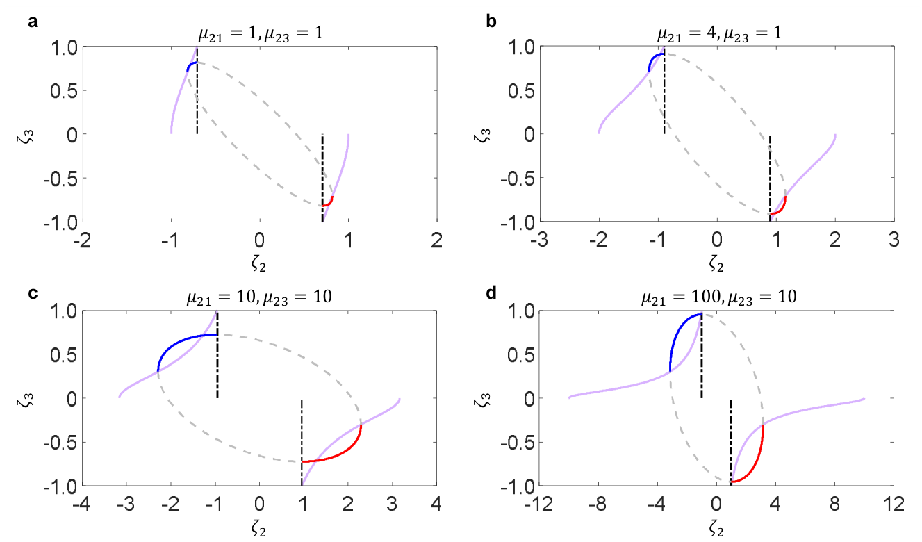
The structural evolution illustrated in Figure 2 demonstrates that the variation of the primary mass ratio () acts as a critical topological driver, completely transforming the geometric landscape of the phase maps and birthing entirely new boundary physics. As progressively scales down, the system deviates from its classical asymptotic baseline and undergoes abrupt, significant topological phase transitions, bifurcating the conventional boundaries into highly nonlinear manifold structures. This mass-driven scaling not only triggers the bifurcation of the continuous trajectories but also reconfigures the pre-existing non-Hermitian pathways into newly emergent topological boundaries. Ultimately, this clearly confirms that the primary mass inertia fundamentally rewrites the underlying topological governance of the semi-definite system. Additionally, the trajectories of CCs characterized by symmetric pairs of negative and positive real double roots are presented in Expanded Data Figure 1.
Figure 3 and Figure 4 present the time signals of the symmetric points for the EPs and CCs, respectively, residing on the identical trajectory. In the analyzed signals, the structural loss associated with complex degenerate roots having a purely negative real part is distinctly demonstrated, alongside the structural gain (Figure 3c and Figure 3e) and its corresponding purely positive real part (Figure 3d and Figure 3f). Figure 3b demonstrates that the amplitude characteristics of the EP increase linearly on a logarithmic scale with the increasing decimal precision of the purely real parameter, which implies that the signal undergoes exponential amplification as the parameter precision scales up.
In contrast to the EP, the signal remains constant at the CC regardless of the increasing decimal precision of the parameter, as verified in Figure 4b. Figure 4c and Figure 4e represent the CC characterized by purely negative real double roots, whereas Figure 4d and Figure 4f exhibit continuously diverging signal characteristics induced by purely positive real double roots. Conclusively, Figure 3 and Figure 4 confirm that the EPs and CCs reside precisely on an identical trajectory, being distinctly demarcated through the phase transition boundary. This pivotal finding rigorously establishes that the EP fundamentally originates from critical damping, successfully bridging the foundational principles of classical physics with the emergent landscapes of modern non-Hermitian physics.
The time-domain responses in Figure 5 elucidate the symmetry and linear divergence mechanism at the purely imaginary degenerate roots. The individual signals for each mass (Figure 5c and Figure 5f) exhibit linear amplification over time, with and maintaining a strict anti-phase relationship due to system symmetry. Conversely, the resulting relative signals (Figure 5d and Figure 5g) demonstrate sustained oscillations with a constant amplitude as the divergence components cancel out. Notably, these relative signals () also display an anti-phase relationship, proving that the intrinsic symmetric phase characteristics of the system are robustly preserved even after divergence cancellation.
Consequently, the algebraic formulations governing the co-existing trajectories of EPs and CCs, which were originally derived for the fixed-free 2DOF damped system [24], are not isolated properties of a specific configuration. Rather, their mathematically generalized universality is validated by the fact that the exact same algebraic derivation mechanism and structural principles consistently manifest in the analysis of a semi-definite 3DOF damped system. This fundamental consistency proves that the interlocking physics between topological singularities and critical dissipation boundary states represents an intrinsic, system-invariant framework rather than an artifact of reduced dimensionality. By establishing this generalized mathematical bridge, this work transcends traditional configuration-specific analysis and provides a robust, scalable paradigm for predicting and controlling stability transitions in higher-order non-Hermitian mechanical systems.
Methods: To accurately map the root trajectories, a variable precision arithmetic (VPA) framework was implemented via MATLAB R2021b with a precision of over 256 significant figures. Perfect degeneracy was verified by constraining the numerical solver until the disparity between the imaginary parts of paired roots disappeared beyond 100 decimal places, ensuring a 100-digit resolution for the governing parameters. This high-precision approach effectively suppressed numerical instabilities at sensitive singular boundaries, preventing artificial truncation errors. For mathematical consistency, a physics-informed tracking algorithm sorted non-real complex roots by their absolute magnitudes and real double roots by their algebraic real values. For computational reproducibility, two distinct parameter sets for the symmetric EPs and CCs are provided in the latter section of the SI.
Mathematical Formulations of System Coefficients
The explicit coefficients governing the characteristic equation in (Eq. (3)) are given as follows:
The explicit coefficients governing the topological phase transition boundary specified in Eq. (4) are defined as follows:
To eliminate the extraneous roots from Eq. (4), which delineates the topological phase transition boundary, the corresponding coefficients (, ) for Eq. (5) are defined as follows:
Author Contributions
Jung Woo Lee conceived the study and led the conceptualization of the framework. Jung Woo Lee and Jin Kim jointly performed the formal theoretical analysis to identify and characterize the properties of EPs and CCs. Jin Kim conducted the systematic investigation and performed the high-precision numerical computations. Jung Woo Lee wrote the manuscript and provided overall supervision of the project. All authors discussed the results and commented on the final manuscript.
Conflicts of Interest
Jung Woo Lee and Jin Kim are inventors on a patent application filed by Kyonggi University related to this work (Korean Patent Application No. 10-2026-0126742).
References
- Wang, C.; Sweeney, W. R.; Stone, A. D.; Yang, L. Coherent perfect absorption at an exceptional point. Science 2021, 373, 1261–1265. [Google Scholar] [CrossRef] [PubMed]
- Ergoktas, M. S.; et al. Topological engineering of terahertz light using electrically tunable exceptional point singularities. Science 2022, 376, 184–188. [Google Scholar] [CrossRef] [PubMed]
- Song, Q.; Odeh, M.; Zúñiga-Pérez, J.; Kanté, B.; Genevet, P. Plasmonic topological metasurface by encircling an exceptional point. Science 2021, 373, 1133–1137. [Google Scholar] [CrossRef] [PubMed]
- Yi, C.; et al. Creating topological exceptional point by on-chip all-dielectric metasurface. Light Sci. Appl. 2025, 14, 262. [Google Scholar] [CrossRef] [PubMed]
- Qin, H.; et al. Sphere of arbitrarily polarized exceptional points with a single planar metasurface. Nat. Commun. 2025, 16, 2656. [Google Scholar] [CrossRef] [PubMed]
- Zhang, M.; et al. Quantum noise theory of exceptional point amplifying sensors. Phys. Rev. Lett. 2019, 123, 180501. [Google Scholar] [CrossRef] [PubMed]
- Lu, Y. -W.; Li, W.; Wang, X. -H. Quantum and classical exceptional points at the nanoscale: Properties and applications. ACS Nano 2025, 19, 17953–17978. [Google Scholar] [CrossRef] [PubMed]
- Doppler, J.; et al. Dynamically encircling an exceptional point for asymmetric mode switching. Nature 2016, 537, 76–79. [Google Scholar] [CrossRef] [PubMed]
- Kononchuk, R.; Cai, J.; Ellis, F.; Thevamaran, R.; Kottos, T. Exceptional-point-based accelerometers with enhanced signal-to-noise ratio. Nature 2022, 607, 697–702. [Google Scholar] [CrossRef] [PubMed]
- Shi, C.; et al. Accessing the exceptional points of parity-time symmetric acoustics. Nat. Commun. 2016, 7, 11110. [Google Scholar] [CrossRef] [PubMed]
- Yoon, J. W.; et al. Time-asymmetric loop around an exceptional point over the full optical communications band. Nature 2018, 562, 86–90. [Google Scholar] [CrossRef] [PubMed]
- Lai, Y. -H.; Lu, Y. -K.; Suh, M. -G.; Yuan, Z.; Vahala, K. Observation of the exceptional-point-enhanced Sagnac effect. Nature 2019, 576, 65–69. [Google Scholar] [CrossRef] [PubMed]
- Hasanli, S.; Hasan, M.; Yoon, H.; Lee, S.; Kim, S. Exceptional points in a passive strip waveguide. Nanophotonics 2025, 14, 1301–1309. [Google Scholar] [CrossRef] [PubMed]
- Peng, B.; et al. Loss-induced suppression and revival of lasing. Science 2014, 346, 328–332. [Google Scholar] [CrossRef] [PubMed]
- Zhen, B.; et al. Spawning rings of exceptional points out of Dirac cones. Nature 2015, 525, 354–358. [Google Scholar] [CrossRef] [PubMed]
- Chen, D. -Y.; Dong, L.; Huang, Q. -A. Inductor-capacitor passive wireless sensors using nonlinear parity-time symmetric configurations. Nat. Commun. 2024, 15, 9312. [Google Scholar] [CrossRef] [PubMed]
- Chang, L.; et al. Parity–time symmetry and variable optical isolation in active–passive-coupled microresonators. Nat. Photonics 2014, 8, 524–529. [Google Scholar] [CrossRef]
- Zhang, J.; et al. A phonon laser operating at an exceptional point. Nat. Photonics 2018, 12, 479–484. [Google Scholar] [CrossRef]
- Wiersig, J. Prospects and fundamental limits in exceptional point-based sensing. Nat. commun. 2020, 11, 2454. [Google Scholar] [CrossRef] [PubMed]
- Suntharalingam, A.; Fernández-Alcázar, L.; Kononchuk, R.; Kottos, T. Noise resilient exceptional-point voltmeters enabled by oscillation quenching phenomena. Nat. Commun. 2023, 14, 5515. [Google Scholar] [CrossRef] [PubMed]
- Hodaei, H.; et al. Enhanced sensitivity at higher-order exceptional points. Nature 2017, 548, 187–191. [Google Scholar] [CrossRef] [PubMed]
- Chen, W.; Özdemir, Ş. K.; Zhao, G.; Wiersig, J.; Yang, L. Exceptional points enhance sensing in an optical microcavity. Nature 2017, 548, 192–196. [Google Scholar] [CrossRef] [PubMed]
- Zhou, H.; et al. Observation of bulk Fermi arc and polarization half charge from paired exceptional points. Science 2018, 359(6379), 1009–1012. [Google Scholar] [CrossRef] [PubMed]
- Kim, J.; Lee, J.W. Preprints ID: 222548; Clusters of loci of innumerable exceptional points in purely real-parameter passive systems: I. Fixed-free 2DOF model. 2026.
- Landers, S.; Tuxbury, W.; Vitebskiy, I.; Kottos, T. Noise-resilient exceptional point sensing with immunity to undesired perturbations. Sci. Adv. 2026, 12, eaeb7018. [Google Scholar] [CrossRef] [PubMed]
- Wang, H.; et al. Exceptional sensitivity near the bistable transition point of a hybrid quantum system. Nat. Phys. 2026, 22, 577–583. [Google Scholar] [CrossRef]
- Zhang, D.; Luo, X. -Q.; Wang, Y. -P.; Li, T. -F.; You, J. Q. Observation of the exceptional point in cavity magnon-polaritons. Nat. commun. 2017, 8, 1368. [Google Scholar] [CrossRef] [PubMed]
- Chen, Y. -Y.; et al. Quantum tomography of a third-order exceptional point in a dissipative trapped ion. Nat. Commun. 2025, 16, 7478. [Google Scholar] [CrossRef] [PubMed]
- Zhang, J.; et al. Exceptional point and hysteresis trajectories in cold Rydberg atomic gases. Nat. Commun. 2025, 16, 3511. [Google Scholar] [CrossRef] [PubMed]
- Patolsky, F.; Zheng, G.; Lieber, C. M. Nanowire sensors for medicine and the life sciences. Nanomedicine 2006, 1, 51–65. [Google Scholar] [CrossRef] [PubMed]
- Assawaworrarit, S.; Yu, X.; Fan, S. Robust wireless power transfer using a nonlinear parity–time-symmetric circuit. Nature 2017, 546, 387–390. [Google Scholar] [CrossRef] [PubMed]
- Miri, M. -A.; Alu, A. Exceptional points in optics and photonics. Science 2019, 363, eaar7709. [Google Scholar] [CrossRef] [PubMed]
- Lee, H.; et al. Chiral exceptional point enhanced active tuning and nonreciprocity in micro-resonators. Light Sci. Appl. 2025, 14, 45. [Google Scholar] [CrossRef] [PubMed]
- Okuma, N.; Sato, M. Non-Hermitian topological phenomena: A review. Annu. Rev. Condens. Matter Phys. 2023, 14, 83–107. [Google Scholar] [CrossRef]
- Ashida, Y.; Gong, Z.; Ueda, M. Non-hermitian physics. Adv. Phys. 2020, 69, 249–435. [Google Scholar] [CrossRef]
- El-Ganainy, R.; et al. Non-Hermitian physics and PT symmetry. Nat. Phys. 2018, 14, 11–19. [Google Scholar] [CrossRef]
- Lau, H. -K.; Clerk, A. A. Fundamental limits and non-reciprocal approaches in non-Hermitian quantum sensing. Nat. commun. 2018, 9, 4320. [Google Scholar] [CrossRef] [PubMed]
- Bender, C. M. Making sense of non-Hermitian Hamiltonians. Rep. Prog. Phys. 2007, 70, 947–1018. [Google Scholar] [CrossRef]
- Wu, Y.; et al. Observation of parity-time symmetry breaking in a single-spin system. Science 2019, 364, 878–880. [Google Scholar] [CrossRef] [PubMed]
- Guo, A.; et al. Observation of PT-symmetry breaking in complex optical potentials. Phys. Rev. Lett. 2009, 103 093902. [Google Scholar]
- Hussein, M. I. Theory of damped Bloch waves in elastic media. Phys. Rev. B 2009, 80, 212301. [Google Scholar] [CrossRef]
- Ding, K.; Fang, C.; Ma, G. Non-Hermitian topology and exceptional-point geometries. Nat. Rev. Phys. 2022, 4, 745–760. [Google Scholar] [CrossRef]
- Brandenbourger, M.; Locsin, X.; Lerner, E.; Coulais, C. Non-reciprocal robotic metamaterials. Nat. commun. 2019, 10, 4608. [Google Scholar] [CrossRef] [PubMed]
- Ghatak, A.; Brandenbourger, M.; Van Wezel, J.; Coulais, C. Observation of non-Hermitian topology and its bulk–edge correspondence in an active mechanical metamaterial. Proc. Natl. Acad. Sci. USA 2020, 117, 29561–29568. [Google Scholar] [CrossRef] [PubMed]
- Bergholtz, E. J.; Budich, J. C.; Kunst, F. K. Exceptional topology of non-Hermitian systems. Rev. Mod. Phys. 2021, 93, 015005. [Google Scholar] [CrossRef]
- Heiss, W. D. The physics of exceptional points. J. Phys. A Math. Theor. 2012, 45, 444016. [Google Scholar] [CrossRef]
- Cummer, S. A.; Christensen, J.; Alù, A. Controlling sound with acoustic metamaterials. Nat. Rev. Mater. 2016, 1, 1–13. [Google Scholar] [CrossRef]
Figure 1.
Topological Homomorphism. a. Schematic of the 3-DOF semi-definite damped system, where the parameters and of the tertiary system are mapped into , , and of the secondary system via the linear coupling manifolds and . b. In the asymptotic limit as , the topological map of the semi-definite system identically converges to that of the single ended 2-DOF system, thereby demonstrating topological invariance. Curve I in panel b represents the envelope of the ellipse and serves as the boundary of critical damping (CC) with purely negative (upper) and positive (lower) real roots; II denotes the boundary of critical damping with purely negative (upper) and positive (lower) real roots; and III indicates the topological phase transition boundary, where its upper boundary represents the threshold of complex degenerate roots (EP) with purely negative real parts, and its lower boundary denotes that of complex degenerate roots with purely positive real parts separated by the trajectory of purely imaginary degenerate roots (IV). The green curves represent the boundaries obtained by setting and in the present study, while the dotted curves indicate the results from the previous study [24].
Figure 1.
Topological Homomorphism. a. Schematic of the 3-DOF semi-definite damped system, where the parameters and of the tertiary system are mapped into , , and of the secondary system via the linear coupling manifolds and . b. In the asymptotic limit as , the topological map of the semi-definite system identically converges to that of the single ended 2-DOF system, thereby demonstrating topological invariance. Curve I in panel b represents the envelope of the ellipse and serves as the boundary of critical damping (CC) with purely negative (upper) and positive (lower) real roots; II denotes the boundary of critical damping with purely negative (upper) and positive (lower) real roots; and III indicates the topological phase transition boundary, where its upper boundary represents the threshold of complex degenerate roots (EP) with purely negative real parts, and its lower boundary denotes that of complex degenerate roots with purely positive real parts separated by the trajectory of purely imaginary degenerate roots (IV). The green curves represent the boundaries obtained by setting and in the present study, while the dotted curves indicate the results from the previous study [24].
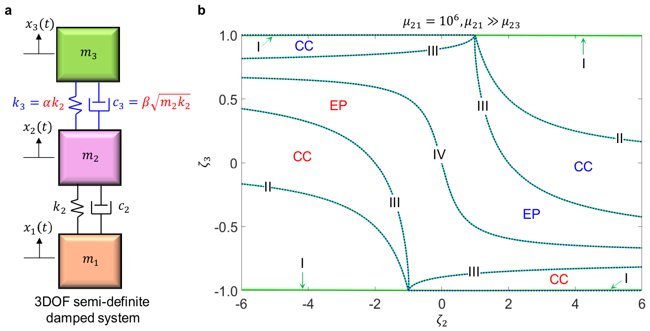
Figure 2.
Continuous Boundary Deformation. The topological phase transition boundaries evolve continuously as a function of the mass ratio (), converging to the L-surface of the fixed-free 2DOF system as the ratio increases (Figure 1b). The evolutionary pathways of several topological maps as a function of are presented in panels a–d. As decreases, the topological maps exhibit abrupt and significant transitions. In these topological maps, the black circular marks denote the discrete points of the purely imaginary complex degenerate roots that intersect with the symmetric pair loci of , while the red and blue circular marks represent the discrete points that define the boundaries of the topological phase transitions. Panel a illustrates the topological map under the conditions = 1 and = 1, where Curve I denotes the boundary of the topological phase transition, and Line II represents the locus satisfying , which serves as the starting point of the phase trajectory. In panel b, Curve III denotes the locus of the purely imaginary complex degenerate roots. In panel c, Curve IV indicates the boundary of the CCs, and in panel d, Curve V represents the envelope of the ellipse.
Figure 2.
Continuous Boundary Deformation. The topological phase transition boundaries evolve continuously as a function of the mass ratio (), converging to the L-surface of the fixed-free 2DOF system as the ratio increases (Figure 1b). The evolutionary pathways of several topological maps as a function of are presented in panels a–d. As decreases, the topological maps exhibit abrupt and significant transitions. In these topological maps, the black circular marks denote the discrete points of the purely imaginary complex degenerate roots that intersect with the symmetric pair loci of , while the red and blue circular marks represent the discrete points that define the boundaries of the topological phase transitions. Panel a illustrates the topological map under the conditions = 1 and = 1, where Curve I denotes the boundary of the topological phase transition, and Line II represents the locus satisfying , which serves as the starting point of the phase trajectory. In panel b, Curve III denotes the locus of the purely imaginary complex degenerate roots. In panel c, Curve IV indicates the boundary of the CCs, and in panel d, Curve V represents the envelope of the ellipse.
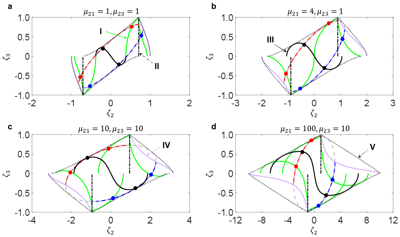
Figure 3.
Time signals at the EPs. a. The star and square markers indicate the exceptional singularities residing on the trajectory of under the conditions = 1 and = 1. b. The output-to-input ratio in response to a constant input at =0 is plotted on a logarithmic scale as a function of the number of decimal places of the real parameters; it demonstrates that the output value increases linearly on a logarithmic scale with the enhancement of numerical precision. Panels c and d present the time signals obtained under the excitation at with an initial displacement , while panels e and f show the time signals obtained under the excitation at . Panels c and e illustrate the structural loss behavior at the star marker (= 0.4), where the complex degenerate roots possess a purely negative real part. Conversely, panels d and f demonstrate the structural gain behavior at the square marker (= -0.4), characterized by a purely positive real part.
Figure 3.
Time signals at the EPs. a. The star and square markers indicate the exceptional singularities residing on the trajectory of under the conditions = 1 and = 1. b. The output-to-input ratio in response to a constant input at =0 is plotted on a logarithmic scale as a function of the number of decimal places of the real parameters; it demonstrates that the output value increases linearly on a logarithmic scale with the enhancement of numerical precision. Panels c and d present the time signals obtained under the excitation at with an initial displacement , while panels e and f show the time signals obtained under the excitation at . Panels c and e illustrate the structural loss behavior at the star marker (= 0.4), where the complex degenerate roots possess a purely negative real part. Conversely, panels d and f demonstrate the structural gain behavior at the square marker (= -0.4), characterized by a purely positive real part.
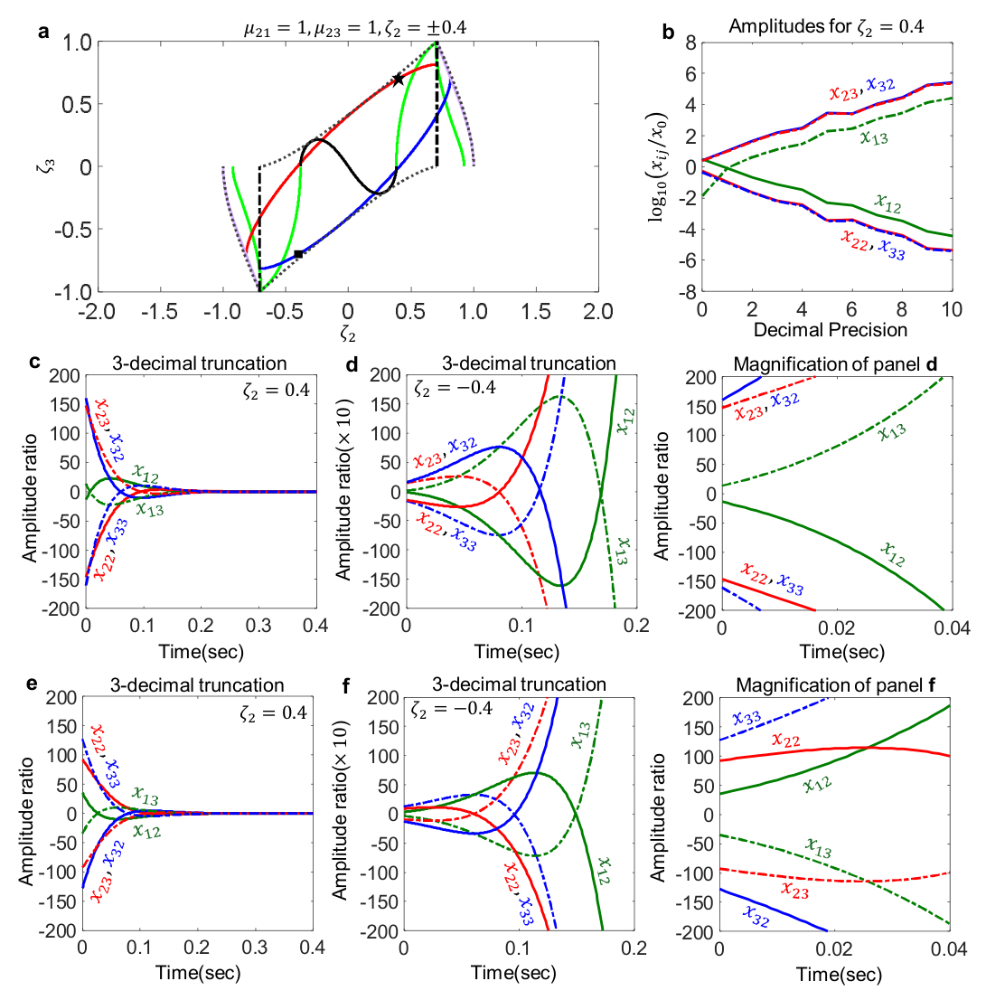
Figure 4.
Time signals at the CCs. a. The CCs (indicated by the star and square markers) located on the same trajectory as in Figure 3 correspond to the state where =0.6. b. The output amplitude relative to the input at =0, expressed as , is plotted on a logarithmic scale. Beyond a precision of three decimal places, the amplitude stabilizes completely, yielding identical values. Panels c–f present the time signals for the CCs obtained at a precision of three decimal places. Specifically, panels c and e correspond to the CCs possessing purely negative real double roots (star marker at = 0.6), while panels d and f represent those possessing purely positive real double roots (square marker at = -0.6). Panels c and d present the time signals obtained by applying an initial displacement to whereas panels e and f show the time signals captured by applying an initial displacement to .
Figure 4.
Time signals at the CCs. a. The CCs (indicated by the star and square markers) located on the same trajectory as in Figure 3 correspond to the state where =0.6. b. The output amplitude relative to the input at =0, expressed as , is plotted on a logarithmic scale. Beyond a precision of three decimal places, the amplitude stabilizes completely, yielding identical values. Panels c–f present the time signals for the CCs obtained at a precision of three decimal places. Specifically, panels c and e correspond to the CCs possessing purely negative real double roots (star marker at = 0.6), while panels d and f represent those possessing purely positive real double roots (square marker at = -0.6). Panels c and d present the time signals obtained by applying an initial displacement to whereas panels e and f show the time signals captured by applying an initial displacement to .
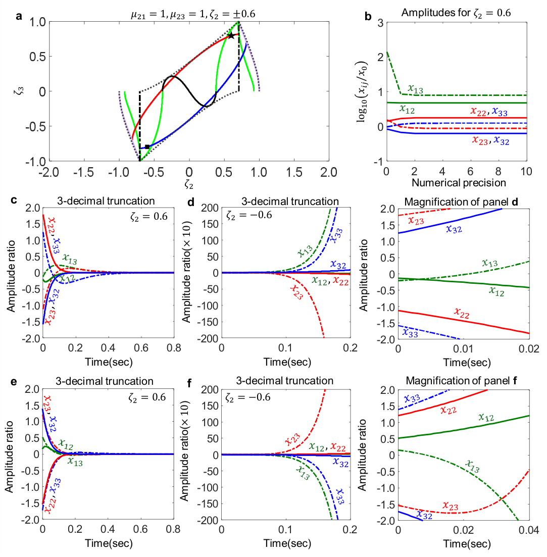
Figure 5.
Time signals at the purely imaginary degenerate roots. Time signals are presented for the two symmetric points where the purely imaginary and the complex degenerate root trajectories meet. Based on the purely imaginary degenerate roots, the lower part consists of complex degenerate roots with purely positive real parts, and the upper part consists of complex degenerate roots with purely negative real parts. a. The two points (the star and square markers) possess purely imaginary degenerate roots. Panels b, c, and d present the results for the star markers, while panels e, f, and g present the results for the square markers. Panels b and e show the signal amplification in terms of amplitude ratio on a logarithmic scale as the decimal precision of the real parameters increases. Panels c and f display the changes in time signals for each mass, and panels d and g present the time signals for the relative displacement . Under an initial excitation of applied to , while all other dynamic characteristics remain identical for both symmetric points, the resulting signals for and exhibit an anti-phase relationship.
Figure 5.
Time signals at the purely imaginary degenerate roots. Time signals are presented for the two symmetric points where the purely imaginary and the complex degenerate root trajectories meet. Based on the purely imaginary degenerate roots, the lower part consists of complex degenerate roots with purely positive real parts, and the upper part consists of complex degenerate roots with purely negative real parts. a. The two points (the star and square markers) possess purely imaginary degenerate roots. Panels b, c, and d present the results for the star markers, while panels e, f, and g present the results for the square markers. Panels b and e show the signal amplification in terms of amplitude ratio on a logarithmic scale as the decimal precision of the real parameters increases. Panels c and f display the changes in time signals for each mass, and panels d and g present the time signals for the relative displacement . Under an initial excitation of applied to , while all other dynamic characteristics remain identical for both symmetric points, the resulting signals for and exhibit an anti-phase relationship.
Expanded Data Figure 1.
Trajectories of paired real double roots at CC points: It is worth noting that while several closely associated trajectory branches are derived concurrently with the results in Figure 2, they have been intentionally isolated and presented in a separate figure. This deliberate omission in the current plot prevents excessive visual crowding and maintains the graphical clarity of the manifold’s core structures.
Expanded Data Figure 1.
Trajectories of paired real double roots at CC points: It is worth noting that while several closely associated trajectory branches are derived concurrently with the results in Figure 2, they have been intentionally isolated and presented in a separate figure. This deliberate omission in the current plot prevents excessive visual crowding and maintains the graphical clarity of the manifold’s core structures.
Disclaimer/Publisher’s Note: The statements, opinions and data contained in all publications are solely those of the individual author(s) and contributor(s) and not of MDPI and/or the editor(s). MDPI and/or the editor(s) disclaim responsibility for any injury to people or property resulting from any ideas, methods, instructions or products referred to in the content. |
© 2026 by the authors. Licensee MDPI, Basel, Switzerland. This article is an open access article distributed under the terms and conditions of the Creative Commons Attribution (CC BY) license (http://creativecommons.org/licenses/by/4.0/).
Copyright: This open access article is published under a Creative Commons CC BY 4.0 license, which permit the free download, distribution, and reuse, provided that the author and preprint are cited in any reuse.