
Submitted:
15 July 2026
Posted:
16 July 2026
You are already at the latest version
Abstract
Unmanned aerial vehicles (UAVs) equipped with lightweight gas sensors offer a promising means of monitoring localized pollutant emissions. However, airflow generated by multirotor propellers can disturb the surrounding atmosphere and affect measured gas concentrations. This study investigates the influence of rotor-induced downwash on vehicle exhaust plume measurements through a combined experimental and numerical approach. Experimental measurements were conducted using a stationary diesel vehicle operating at idle, while a propeller-based system reproduced UAV downwash at heights between 0.5 and 5.5 m above a fixed CO2 sensor. A low-cost Feather-based sensing platform was evaluated against a commercial IoTSens monitoring station. Complementary CFD simulations were performed in OpenFOAM using a compressible multi-species solver, Large Eddy Simulation (LES), and a Multiple Reference Frame (MRF) approach. Experimental measurements showed CO2 reductions of up to 52.7%, while CFD predicted reductions between 50.4% and 88.5%. Both approaches identified a transition in plume–wake interaction, with the strongest effects occurring below approximately 2–3 m. These findings demonstrate that UAV height is a critical parameter affecting gas-sensing accuracy and should be considered when designing UAV-based environmental monitoring missions.
Keywords:
UAV-based sensing
; CO2 monitoring
; vehicle exhaust plume
; rotor-induced flow
; air pollution monitoring
; computational fluid dynamics
; environmental sensing
1. Introduction
Air pollution remains one of the most significant environmental and public health challenges worldwide because it is associated with numerous diseases and accounts for millions of premature deaths each year [1].
Poor air quality has been associated with numerous adverse health outcomes, establishing air pollution as one of the most pressing public health challenges worldwide while atmospheric pollutants such as methane and other greenhouse gases play a crucial role in climate change dynamics [2,3]. In this context, accurate monitoring of gaseous pollutants is essential not only for understanding emission sources but also for supporting mitigation strategies and policy decisions [3].
Despite its importance, environmental monitoring still faces significant technological limitations. Traditional air quality monitoring systems rely on fixed ground stations or manual sampling, which cannot provide continuous measurements across all locations and time periods and are often costly to install, operate, and maintain leading to insufficient spatial and temporal resolution [2,3]. Furthermore, these stationary systems are limited in their ability to capture vertical distributions of pollutants, leaving a sampling gap between ground level and low-altitude atmospheric layers [3]. As a result, capturing the highly dynamic behavior of pollutant plumes, especially in urban environments or near emission sources, remains a challenging task.
In recent years, unmanned aerial vehicles (UAVs) have emerged as a promising solution to overcome these limitations. Advances in UAV technology, have created new opportunities for quantifying atmospheric emissions enabling flexible, high-resolution measurements at different locations and altitudes [3]. UAV-based systems provide high operational flexibility and maneuverability and allow access to hazardous or hard-to-reach environments, while enabling three-dimensional mapping and real-time monitoring of pollutant dispersion [2,4]. These capabilities make UAV platforms particularly suitable for applications such as industrial emissions monitoring, urban air quality assessment, and emergency response scenarios.
At the same time, the development of gas sensing technologies has evolved toward compact, low-cost, and energy-efficient solutions. Miniaturized sensors—including MOS, electrochemical, and nondispersive infrared (NDIR) devices—have enabled the integration of multi-gas sensing platforms into lightweight UAV systems [3,5,6,7]. This evolution has significantly expanded the accessibility of air quality monitoring, allowing the deployment of distributed sensing systems at reduced cost. However, the adoption of low-cost sensors also introduces new challenges, as low-cost sensors typically exhibit reduced accuracy and require careful calibration due to environmental sensitivities and cross-interference effects [4,8,9].
A critical challenge in UAV-based gas sensing arises from the interaction between the drone and the surrounding airflow. The concentration measured by a UAV-mounted gas sensor is not determined solely by the characteristics of the emission source but is also influenced by the aerodynamic interaction between the rotor wake and the surrounding gas plume. Rotor-induced airflow alters plume transport by modifying entrainment, turbulent mixing, and dilution processes, potentially causing the concentration measured by the sensor to differ significantly from the actual concentration field surrounding the emission source. Previous studies have shown that measurements obtained by in situ sensors are highly sensitive to atmospheric turbulence and that sampling accuracy can be degraded due to gas dilution and mixing effects caused by the propellers [7,10]. These disturbances complicate the interpretation of measurements and highlight the importance of both sensor placement and flight configuration in ensuring reliable data acquisition. [11]. Despite growing interest in UAV-based atmospheric monitoring, relatively few studies have quantitatively combined controlled experimental measurements and CFD simulations to investigate how rotor-induced downwash modifies measured gas concentrations near localized emission sources. Most previous investigations have focused on UAV aerodynamics, sensor placement, or platform design rather than on the direct quantification of measurement bias caused by rotor–plume interactions.
More recently, several researchers have employed Computational Fluid Dynamics (CFD) to investigate the aerodynamic effects of UAV operation on atmospheric sampling systems. Roldán et al. [12] combined CFD simulations and experimental measurements to identify optimal sensor locations on a quadrotor platform, demonstrating that rotor-induced airflow can influence environmental measurements if sensors are positioned within regions of elevated velocity. Similarly, Yilmaz and Hu [13] used CFD to characterize the aerodynamic behavior of quadcopters under hovering conditions and reported the formation of strong velocity gradients and recirculation structures beneath the propellers. More recently, Kong et al. [14] employed CFD simulations to evaluate airflow disturbances around a rotary-wing UAV used for air-pollutant monitoring, identifying substantial differences in the airflow field depending on the operational state of the aircraft. These studies consistently indicate that rotor-induced flow may significantly influence the quality and representativeness of atmospheric measurements.
Despite these advances, the interaction between UAV downwash and gas plumes remains only partially understood. Marturano et al. [15] demonstrated through multiphase CFD simulations that the turbulence generated by drone propellers can strongly affect gas detection performance and measured concentrations. Likewise, Schuyler and Guzman [16] highlighted that only a limited number of studies have explicitly investigated the influence of rotor turbulence on trace-gas measurements, despite the growing adoption of UAV-based atmospheric sensing systems. More recently, Park et al. [17] showed that rotor-induced recirculation can either enhance or suppress the detection of gaseous pollutants depending on the hovering altitude and the interaction between the downwash and the target plume. Their results suggest that rotor wash does not merely act as a source of measurement uncertainty but actively modifies plume transport, mixing, and dilution.
Although UAV-based gas sensing systems offer unique capabilities for real-time, high-resolution spatial monitoring, their performance remains constrained by payload limitations, flight time, and measurement uncertainties arising from rotor-induced airflow and environmental conditions. The central challenge is therefore not only the integration of lightweight, low-power, and high-precision sensors, but also the development of reliable sampling strategies that minimize measurement bias. In practical environmental monitoring, this issue is particularly important because measured gas concentrations are frequently used to estimate pollutant emissions, identify leak locations, and assess environmental impacts. Consequently, understanding when rotor-induced mixing becomes the dominant mechanism affecting measured concentrations is essential for developing reliable UAV-based sensing methodologies.
In parallel, UAV-mounted greenhouse-gas sensors have demonstrated considerable potential for environmental monitoring applications. Kahn et al. [18] developed lightweight laser-based sensors capable of measuring carbon dioxide (CO2), CH4, and H2O (as water vapor) with sub-percent precision from UAV platforms, enabling high-spatial-resolution observations of atmospheric trace gases. Similarly, Berman et al. [19] integrated a compact atmospheric gas analyzer into a UAV platform and demonstrated reliable measurements of greenhouse gases at low altitudes and in remote environments. As UAV-based gas sensing systems have matured, increasing attention has been directed toward the influence of sensor placement and rotor-induced airflow on measurement quality. Several studies have identified regions above or laterally offset from the airframe as preferable sensor locations because they experience lower aerodynamic disturbance than locations directly beneath the rotors [20,21,22]. Likewise, experimental and numerical investigations have shown that propeller wake can significantly modify gas transport by dispersing plumes, altering the concentration reaching the sensor, and generating strong turbulence gradients around the platform [22,23,24]. These findings suggest that the measured concentration may depend not only on the emission source itself but also on the relative position of the sensor within the UAV-induced flow field. Consequently, uncertainty remains regarding the minimum separation distances required to avoid measurement distortion when monitoring localized emission sources.
Given the difficulty of directly observing rotor–plume interactions experimentally, numerical modeling techniques such as CFD have become valuable tools for investigating the mechanisms responsible for measurement bias in UAV-based sensing systems. CFD enables detailed visualization of plume transport, turbulent mixing, recirculation regions, and rotor-induced entrainment, providing information that is often inaccessible through field measurements alone. Recent studies have successfully employed CFD to identify low-disturbance sensor locations, characterize UAV wake structures, and evaluate the influence of different flight conditions on atmospheric sampling performance [21,22,25,26]. However, several authors have emphasized the importance of validating CFD predictions using experimental observations because concentration transport and near-body flow structures remain challenging to reproduce accurately using numerical models alone [22,26,27]. Despite these advances, relatively few investigations have combined controlled experiments with CFD simulations to quantitatively assess how rotor-induced flow modifies gas concentration measurements near localized vehicle exhaust sources. Consequently, an important research question remains unresolved: to what extent does UAV-induced downwash alter the concentration measured by a gas sensor positioned near a localized emission source, and at what separation distance does rotor-induced mixing become the dominant mechanism controlling plume dilution?
Motivated by these challenges, this work investigates the performance of a low-cost Feather-based gas sensing system for UAV-assisted environmental monitoring. CO2 was selected as the target species in the present study because it is continuously emitted by combustion engines, can be measured accurately using compact nondispersive infrared (NDIR) sensors, and behaves as a suitable tracer gas for investigating plume transport and dilution processes. Moreover, the widespread use of CO2 monitoring in environmental studies facilitates direct comparison with previous investigations of UAV-based gas sensing. To assess the reliability of the proposed platform, its measurements are validated against those obtained with a commercial IoTSens gas sensing system, which serves as a reference instrument. Measurements are conducted using the exhaust plume of a diesel vehicle as a controlled pollution source, enabling a direct comparison between the low-cost and commercial systems under realistic conditions. To evaluate the influence of UAV-induced airflow on sensor readings, experiments are performed at multiple drone–sensor separation distances (50–550 cm). Additionally, three of the experimental configurations (50, 150, and 250 cm) are reproduced, and three additional configurations (100, 200, and 300 cm) are investigated using CFD simulations in OpenFOAM to provide a detailed characterization of rotor-induced plume transport. Accordingly, this study addresses the following research questions:
- How does UAV height influence the CO₂ concentration measured near a vehicle exhaust plume?
- Can Large Eddy Simulation (LES) reproduce the principal concentration reductions observed experimentally?
- Which flow mechanisms govern rotor-induced plume dilution and entrainment?
- What UAV operating distances minimize measurement distortion while preserving sensing capability?
To answer these questions, the main contributions of this work are fourfold:
- Experimental quantification of UAV-induced measurement bias during vehicle exhaust monitoring under controlled operating conditions.
- Validation of a low-cost Feather-based sensing platform against a commercial IoTSens monitoring station.
- Application of LES-based CFD simulations to visualize and explain rotor–plume interactions that cannot be directly observed experimentally.
- Identification of UAV operating conditions under which rotor-induced mixing becomes the dominant mechanism controlling measured CO2 concentrations.
To address the identified research questions, this study combines controlled experiments with LES to investigate how rotor-induced downwash influences CO2 concentrations measured near a vehicle exhaust plume. The proposed methodology provides both quantitative measurements and detailed flow-field information, enabling a comprehensive assessment of plume–wake interactions relevant to UAV-based environmental monitoring.
Although the present study focuses on vehicle exhaust emissions, the proposed methodology is applicable to a broader range of UAV-based environmental monitoring scenarios involving localized gaseous emissions, including industrial sources, fugitive emissions, and leak detection applications.
2. Materials and Methods
This study employed a combined experimental and numerical methodology to investigate the influence of UAV-induced downwash on the transport and detection of vehicle exhaust emissions. Controlled experiments were conducted using the exhaust plume of a stationary diesel passenger vehicle operating at idle conditions as a reproducible CO2 source. CO2 concentrations were measured using both a low-cost Feather-based sensing platform and a commercial IoTSens air-quality monitoring station. Complementary CFD simulations based on LES were subsequently performed to characterize the flow structures governing rotor–plume interactions and to support the interpretation of the experimental observations.
2.1. Experimental Setup
An experimental campaign was conducted to investigate the influence of UAV-induced airflow on the dispersion and detection of vehicle exhaust emissions. The experiments were performed using a stationary Hyundai i30 passenger vehicle equipped with a 1.6 L CRDi diesel engine operating under constant idle conditions as a controlled CO2 emission source. A propeller-driven aerial system was positioned at different heights above a fixed sensing location to reproduce the aerodynamic effects of UAV downwash.
Under idle operating conditions, diesel engines of this class typically exhibit exhaust mass flow rates between 0.02 and 0.05 kg s⁻¹, exhaust temperatures ranging from 120 to 180 °C, and tailpipe diameters of approximately 55–60 mm. These representative operating conditions were used to define the inlet boundary conditions for the CFD simulations. The vehicle remained stationary and operated under constant idle conditions throughout the experimental campaign to ensure repeatable measurements.
To minimize the influence of ambient wind and external disturbances, all experiments were conducted in a parking area surrounded by buildings of the Institute of Physical and Information Technologies (ITEFI) of the Spanish National Research Council, which provided effective shielding from large-scale atmospheric currents. The gas sensor was positioned 1 m downstream of the tailpipe outlet and approximately 5 cm above the ground, and this location was maintained for all experiments to enable direct comparison between the different UAV operating heights. Figure 1 illustrates the experimental setup for two representative rotor positions (1.5 and 5.5 m) together with a close-up of the sensing systems.
2.1.1. Propeller System
To reproduce the aerodynamic effects generated by a hovering UAV, a custom-built dual-propeller system was constructed. The setup consisted of two brushless electric motors (A2212-13T, 1000 KV) driving a pair of 25.4 cm-diameter propellers through electronic speed controllers. Motor speed was regulated using a 33-step throttle controller, yielding an estimated maximum rotational speed of approximately 11,100 rpm when supplied at 11.1 V. The entire system was managed by an Arduino Uno R4 Wi-Fi board, which coordinated throttle commands and ensured synchronized operation of both motors.
Three operating conditions were investigated:
- Low speed (Throttle level 18): approximately 6,500 rpm;
- Medium speed (Throttle level 22): approximately 8,000 rpm;
- High speed (Throttle level 28): approximately 10,000 rpm.
These values were selected to represent the range of rotor speeds typically encountered in hovering multirotor UAVs, where propeller rotational velocities commonly approach 10,000 rpm.
2.1.2. Sensor Instrumentation
Two independent sensing systems were used during the experimental campaign.
The primary measurement system consisted of an Adafruit Feather M0 WiFi - ATSAMD21 board equipped with a Sensirion (Sensirion AG, Stäfa, Switzerland) SCD41-D-R2 sensor operating in single-shot mode [28]. The sensor measures CO₂ concentrations between 400 and 5,000 ppm with an accuracy of ±(50 ppm + 2.5%) and a repeatability of ±10 ppm. In addition to CO2, the sensor records ambient temperature and relative humidity.
To provide an independent reference measurement, a commercial IoTsens Air Quality Monitor (IoTsens, Grupo Gimeno, Castellón, Spain) was simultaneously deployed. This instrument measures CO2, CO, NO, NO2, SO2, O3, H2S, particulate matter (PM1, PM2.5 and PM10), total volatile organic compounds (TVOC), temperature, and relative humidity. The IoTsens device was not used to calibrate the Feather-based sensor; rather, it served as an independent reference instrument for comparison and validation of the recorded CO2 trends. Using both systems simultaneously allowed assessment of the influence of sensor exposure conditions and housing design on the measured concentrations.
The Feather-based system was directly exposed to the surrounding air, whereas the IoTsens station operated inside a weather-protected enclosure designed for long-term outdoor deployment. This difference in sensor exposure was considered when interpreting the recorded concentration levels.
2.1.3. Experimental Matrix and Procedure
The influence of rotor-induced airflow on exhaust-plume detection was investigated by positioning the propeller system directly above the sensing location. Six vertical separation distances between the propeller system and the sensor were evaluated: 0.5, 1.5, 2.5, 3.5, 4.5, and 5.5 m. At each height, measurements were performed at propeller rotational speeds of approximately 6,500 rpm and 10,000 rpm. To investigate the effect of an intermediate operating condition, additional measurements at approximately 8,000 rpm were conducted for the highest (5.5 m) and lowest (0.5 m) rotor positions. Reference measurements were also acquired without rotor operation to characterize the undisturbed exhaust plume and establish baseline CO2 concentrations.
The experimental campaign was conducted sequentially, beginning with the highest rotor elevation and progressively reducing the separation distance between the propeller system and the sensing location. Each test condition was maintained for approximately 20 min, allowing the CO2 sensors to reach stable readings while capturing the temporal variability associated with both the vehicle exhaust plume and the rotor-induced airflow. Between consecutive tests, the propellers were switched off and background CO2 measurements were recorded to allow ambient conditions to recover and minimize potential interference between successive operating conditions. Table 1 summarizes the experimental matrix.
2.1.4. Data Processing
Data from the IoTsens monitoring station were transmitted through a LoRaWAN communication network and stored on the ThingSpeak cloud platform. The Feather-based sensing system transmitted data via Wi-Fi to the same platform, allowing synchronized storage and subsequent analysis.
The collected time-series data were segmented according to the experimental schedule. Periods associated with changes in rotor height, motor speed adjustments, and preliminary equipment checks were excluded from further analysis. In addition, at every transition between operating conditions, the first 20 recorded values (approximately 150 s) were removed. This exclusion period allowed the sensors to clear residual concentrations, avoid transient saturation effects, and stabilize before data were used for quantitative comparison.
The primary variables analyzed were:
- Mean CO2 concentration;
- Maximum CO2 concentration;
- Temporal concentration variability;
- Relative concentration changes with respect to the no-drone condition.
These experimental measurements were subsequently compared with the CFD simulations to evaluate whether the numerical model was capable of reproducing the observed effects of rotor-induced airflow on CO2 plume dispersion and dilution.
2.2. Numerical Framework
The numerical simulations were performed using OpenFOAM v12 (OpenCFD Ltd., UK), an open-source finite-volume CFD framework. The transient multicomponentFluid solver was employed to simulate the transient transport of a compressible gas mixture composed of atmospheric air and CO2. The solver is based on the finite-volume discretization of the governing conservation equations and uses the PIMPLE algorithm, a hybrid PISO–SIMPLE approach, to achieve stable pressure–velocity coupling in transient simulations [29].
The objective of the numerical study was to investigate the influence of UAV-induced downwash on the dispersion of a CO2 plume. Consequently, no combustion, chemical reactions, or species generation mechanisms were considered. Carbon dioxide was therefore treated as a passively transported species, with its concentration evolving solely through advection, diffusion, and turbulent mixing within the flow field.
Turbulence was resolved using a LES approach. The one-equation kEqn subgrid-scale model was selected to represent the effects of unresolved turbulent structures on the resolved scales [30]. This approach enables the direct resolution of the dominant flow structures generated by the interaction between the exhaust plume and the rotor-induced airflow while modelling only the smallest turbulent scales.
The UAV propellers were represented using the Multiple Reference Frame (MRF) approach. Two independent rotating zones were defined, each corresponding to one propeller, each operating at a rotational speed of 6500 rpm (ω=680.68 rad s−1). The MRF methodology provides a computationally efficient representation of the rotor-induced flow field while maintaining reasonable accuracy for the prediction of plume–downwash interactions.
2.2.1. Governing Equations
The multicomponentFluid solver computes the conservation equations of mass, momentum, and species transport for compressible multicomponent fluids [29]. Since chemical reactions were not considered in this work, the species source terms were set to zero and the transport of CO2 was governed solely by convection and diffusion.
The governing equations solved by the multicomponentFluid solver include:
Continuity equation
Momentum equation
where ρ is density, u is velocity, p is pressure, τ is the viscous stress tensor, SMRF represents source terms associated with the rotating reference frames used to model the UAV propellers.
The viscous stress tensor is defined as:
where μ is the dynamic viscosity and I is the identity tensor.
Species transport equation
For each transported species, the conservation equation is:
where Yi is the mass fraction of species i and Vi is the diffusion velocity. Since no chemical reactions were included, the species production term is equal to zero.
The diffusion velocity follows Fick's law:
where Di,mix is the mixture-averaged diffusion coefficient and Xi is the mole fraction of species i.
The transported species considered in this work were atmospheric air and CO2. The resulting concentration field was used to evaluate the influence of UAV downwash on exhaust-plume dispersion and the concentration measured at the sensor location.
2.2.2. Computational Domain and Geometry
The computational domain consisted of a three-dimensional rectangular enclosure representing a semi-open atmospheric environment surrounding the vehicle exhaust plume and the UAV. The domain dimensions were 3.0 m × 3.5 m × 3.0 m (length × height × width), providing sufficient space for plume development while limiting computational cost. Figure 2 shows the computational domain.
A simplified UAV geometry was employed, consisting of the drone frame and two 25.4 cm propellers represented as triangulated STL surfaces. The propellers were modelled using Multiple Reference Frame (MRF) zones to reproduce the rotor-induced airflow.
The exhaust source was modeled using a square inlet positioned 30 cm above the ground at the center of the domain. A square geometry was selected to simplify the meshing process, as it minimizes mesh-quality issues—such as excessive skewness, non-orthogonality, and abrupt cell-transition gradients—between the inlet patch and the surrounding internal mesh. Through this inlet, an air– CO2 mixture (0.92 and 0.08 by volume, respectively) was injected to emulate the exhaust plume produced by a diesel passenger vehicle operating at idle. To represent the rear section of the vehicle and its influence on the local flow field, a fixed wall measuring 1.5 m in height and 1.5 m in width was placed upstream of the exhaust outlet.
To investigate the influence of UAV downwash on plume dispersion and sensor measurements, the drone was positioned at six different heights above the sensor location: 0.5, 1.0, 1.5, 2.0, 2.5, and 3.0 m, hereafter referred to as H1–H6, respectively. The sensor position was maintained fixed throughout all simulations, corresponding to the location used during the experimental campaign.
Although the experimental campaign investigated UAV heights up to 5.5 m, the numerical analysis was limited to heights between 0.5 and 3.0 m because LES simulations are computationally expensive and the strongest experimentally observed concentration reductions occurred within this range. Consequently, the CFD simulations focused on the operating conditions where rotor-induced plume disturbance was expected to be most significant. The highest simulated configuration maintained approximately 0.5 m of clearance between the UAV and the upper boundary of the computational domain.
The numerical campaign focused on the 0.5–3.0 m range because experimental measurements showed that the most significant CO2 concentration reductions occurred at lower UAV heights, whereas the higher-altitude cases exhibited substantially weaker downwash effects. Consequently, the simulations were designed to investigate the region where plume disturbance was expected to be most pronounced.
2.2.3. Boundary Conditions
Boundary conditions were selected to reproduce an isolated vehicle exhaust plume under quiescent atmospheric conditions while allowing free exchange of mass, momentum, and species at the open boundaries.
The boundary conditions used in this study are listed in Table 2.
The exhaust outlet was prescribed as a velocity inlet representing the tailpipe of a diesel vehicle operating at idle conditions. A constant inlet velocity of 3 m s⁻¹ was imposed along the streamwise direction, together with an elevated CO₂ concentration and temperature (324° K) representative of exhaust gases. The injected mixture consisted of air and CO2 with mass fractions of 0.92 and 0.08, respectively, reproducing typical idle-condition exhaust composition.
The top and lateral boundaries of the computational domain were treated as atmospheric openings using the inletOutlet boundary condition for velocity, temperature, turbulent kinetic energy and species concentrations. This treatment behaves as a zero-gradient outlet whenever the flow leaves the domain and imposes prescribed ambient values during reverse flow. Consequently, the plume and the rotor wake were allowed to freely enter and exit the computational domain without requiring specification of an external wind field.
Ambient conditions were prescribed at the open boundaries as Tamb=304° K and YCO2,amb=4.2×10⁻⁴, corresponding to an background atmospheric concentration of approximately 420 ppm CO₂. A static pressure of p=101.6 kPa was imposed at the open boundaries. The remaining surfaces employed a fixedFluxPressure condition to ensure consistency between pressure and momentum conservation.
All solid surfaces, including the rear vehicle wall, UAV frame and propeller surfaces, were modelled using no-slip velocity conditions. Temperature and species concentrations at these surfaces were prescribed using zero-gradient boundary conditions, assuming negligible heat transfer and species generation from the solid boundaries. Figure 3 shows the computational geometry and boundary conditions.
2.2.4. Turbulence Modelling
The interaction between the vehicle exhaust plume and the UAV-induced downwash was simulated using a LES approach. LES explicitly resolves the large, energy-containing turbulent structures while modelling only the unresolved sub-grid scales. Compared with Reynolds-Averaged Navier–Stokes (RANS) approaches, LES provides a more detailed representation of transient flow structures and turbulent mixing, making it particularly suitable for plume dispersion, wake development, and rotor–flow interaction studies [31,32].
The simulations employed the one-equation kEqn sub-grid scale (SGS) model available in OpenFOAM [29]. This model solves a transport equation for the sub-grid turbulent kinetic energy and calculates the corresponding turbulent viscosity from the local SGS energy content [30]. The kEqn formulation offers a suitable balance between computational cost and predictive capability for highly turbulent environmental flows involving plume transport and wake interactions.
Turbulence conditions at the exhaust inlet were prescribed through a fixed turbulent kinetic energy of k=0.09 m2 s−2 together with a characteristic turbulence mixing length of L=0.003 m.
These parameters were selected to represent the turbulent nature of the exhaust flow and were used to initialize the turbulence field leaving the emission source. The prescribed mixing length corresponds to the characteristic scale of the turbulent structures generated at the exhaust outlet and promotes realistic turbulent diffusion during the initial stages of plume development.
Near-wall turbulence was represented using the standard OpenFOAM LES wall treatments nutkWallFunction and kqRWallFunction [29]. These wall functions model the unresolved turbulence within the near-wall region while avoiding the extremely fine mesh requirements needed to fully resolve the viscous sublayer. Consequently, they provide an efficient and widely adopted approach for LES simulations of engineering flows involving solid boundaries.
In addition, the turbulent thermal diffusivity at solid surfaces was modelled using the compressible::alphatWallFunction with a turbulent Prandtl number of Prt=0.85 to account for turbulent heat transfer between the fluid and solid surfaces and to ensure consistency between the momentum and thermal transport models employed throughout the simulations.
2.2.5. Rotating Propeller Representation
The aerodynamic influence of the UAV propellers was represented using the Multiple Reference Frame (MRF) approach [33]. Among the available CFD techniques for modelling rotating machinery, the two methodologies most commonly employed to reproduce the three-dimensional flow generated by rotating blades are the MRF and sliding mesh approaches [34].
In the MRF approach, the rotational motion of the propeller is introduced through a rotating reference frame, allowing the effects of blade rotation to be incorporated directly into the governing equations without physically moving the mesh. Consequently, the flow field is solved as a steady rotating problem, resulting in a significantly lower computational cost than transient moving-mesh techniques. Previous studies have successfully applied the MRF formulation to propeller aerodynamics, demonstrating good agreement with experimental measurements while maintaining reasonable computational requirements [35,36].
By contrast, the sliding mesh method explicitly models the relative motion between rotating and stationary regions through dynamic mesh updates and non-conformal interfaces. Although this approach can provide a more detailed representation of transient blade–flow interactions, it requires substantially greater computational resources because the mesh must be updated at every timestep and the flow solution must be obtained in a fully transient manner. Consequently, sliding mesh techniques are typically employed in studies focused on detailed blade aerodynamics or rotor performance prediction [37,38].
For the present study, the primary objective was to evaluate the influence of rotor-induced downwash on exhaust-plume dispersion rather than to predict propeller thrust or blade aerodynamic performance. Therefore, the MRF methodology was selected because it provides an efficient and sufficiently accurate representation of the mean rotor wake while avoiding the considerable computational expense associated with transient moving-mesh approaches.
Two cylindrical rotating regions were created around the propellers and defined as independent MRF zones. Within these regions, additional source terms were introduced into the momentum equations to account for rotational effects.
The rotational speed was prescribed as N=6500 rpm, which corresponds to ω=680.7 rad s−1. CFD simulations were restricted to the 6500 rpm condition because it provided the best overlap with the investigated height range while reducing computational cost.
2.2.6. Mesh Generation
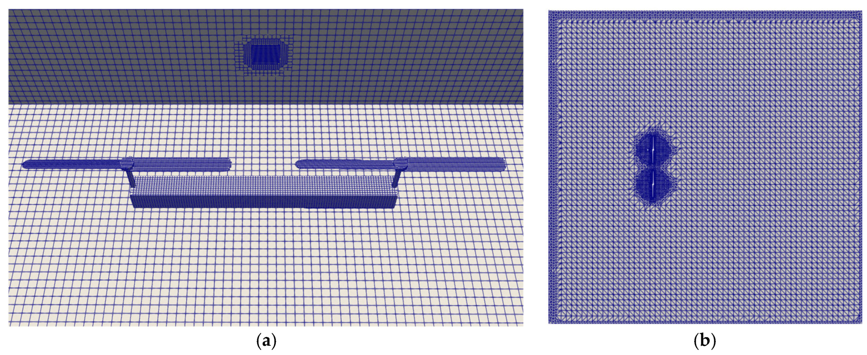
The computational mesh was generated using a hybrid meshing strategy based on the OpenFOAM utilities blockMesh and snappyHexMesh. Initially, a structured hexahedral background mesh was created using blockMesh. This hybrid meshing strategy combines the robustness of a structured background mesh with local body-fitted refinement around complex geometries, providing accurate resolution of the rotor and exhaust regions while maintaining computational efficiency. Subsequently, local refinements were introduced using snappyHexMesh to accurately represent the UAV geometry, exhaust inlet, and rotating regions associated with the propellers.
Surface feature extraction was disabled because the STL geometries contained open and non-manifold surfaces. Local refinement was applied in regions expected to exhibit strong velocity gradients and significant plume–flow interactions, including the exhaust outlet (simulation inlet); the UAV frame; the propeller regions; the MRF zones surrounding the propellers.
To reduce computational cost, progressively coarser cells were employed away from the regions of interest. Two cylindrical cell zones were generated to define the Multiple Reference Frame (MRF) regions associated with the rotating propellers.
The final mesh of the reference configuration contained approximately 457,000 control volumes. Figure 3 illustrates the generated mesh and the location of the MRF zones.
Figure 4.
Mesh (a) Propellers and inlet in the back (b) Plane view of MRF zone.
2.2.7. Mesh Independency Study
A mesh independence study was conducted to evaluate the sensitivity of the numerical solution to mesh resolution and to ensure that the predicted results were not significantly affected by discretization errors [39]. Such studies are a standard verification procedure in CFD and provide confidence that the numerical solution is sufficiently independent of the computational grid. To reduce computational cost, the analysis was performed using the base geometry without the MRF zones while maintaining the same inlet, outlet, and wall boundary conditions used in the production simulations.
Four progressively refined meshes were generated and simulated for 5 s of physical time. Figure 5 presents the lower region of each mesh, highlighting the refinement strategy applied around the exhaust inlet.
To evaluate convergence, the velocity magnitude was sampled along a line extending from the exhaust inlet toward the opposite wall. The first velocity peak along this profile, located in the region most strongly influenced by the developing flow, was selected as the comparison metric. Figure 6 illustrates the velocity profile and the location of the extracted peak.
A refinement level (r) of 1.2 was utilized between successive meshes. Table 3 summarizes the characteristics of each mesh, including total cell count, maximum skewness, and the velocity magnitude extracted from the first peak.
To quantify discretization uncertainty, the velocity values from the first three meshes were used to compute the order of convergence and the Richardson-extrapolated solution. The extrapolated value was then compared with the finest-mesh result to obtain the RDE, which measures the deviation of the numerical solution from the exact Richardson-extrapolated value.
The observed order of convergence (also referred to as order of accuracy) was calculated using the first three mesh levels according to [39]:
where M1, M2, and M3 denote the extracted velocity magnitudes from the coarse, medium, and fine meshes, respectively, and r is the refinement ratio.
The order of accuracy (p) equals 4.31. Richardson extrapolation [41] was subsequently applied to estimate the asymptotic solution:
The extrapolated value was subsequently compared with the solution obtained on the finest mesh, allowing calculation of the RDE, a measure of how far the numerical prediction lies from the exact solution [40]:
The obtained value for M0 was 3.01157, and comparison with mesh 4 (3.02585) yielded a Relative Discretization Error of 0.47%. This low RDE indicates that discretization errors were negligible for meshes larger than approximately 4×10⁵ cells. In addition, only minor variations in the extracted velocity magnitude were observed across the four mesh levels, confirming mesh-independent behavior. Accordingly, the mesh resolution adopted for the production simulations was deemed sufficiently accurate for the objectives of the present study.
2.2.8. Final Simulation Meshes
Following the mesh independence analysis, snappyHexMesh was used to generate the meshes for all UAV-height configurations. Owing to slight geometric differences introduced by the displacement of the UAV and its associated MRF zones, the final cell count varied slightly between cases. Nevertheless, all meshes satisfied OpenFOAM quality criteria, with maximum skewness values below 4 and maximum non-orthogonality values below 65. The final meshes utilized in this study are shown in Table 4.
2.2.9. Numerical Schemes and Solver Settings
The governing equations were discretized using the finite-volume method implemented in OpenFOAM v12. Temporal derivatives were discretized using the localEuler scheme, while spatial gradients were evaluated using the Gauss linear formulation. Diffusive terms were discretized using the Gauss linear corrected scheme, and bounded second-order limitedLinear schemes were employed for the convective terms to ensure numerical stability while minimizing numerical diffusion.
Pressure–velocity coupling was achieved using the PIMPLE algorithm, consisting of one outer correction loop and three pressure-correction iterations per timestep. Adaptive time stepping was employed throughout the simulations [29]. The timestep was automatically adjusted to maintain a maximum Courant number of Comax=3 while the maximum allowable timestep was limited to Δtmax=5×10⁻⁵ s [42].
These settings provided a stable solution while maintaining sufficient temporal resolution to capture the transient interaction between the UAV-induced downwash and the exhaust plume.
Pressure, momentum, turbulence, and species equations were solved using the standard iterative linear solvers available in OpenFOAM with convergence tolerances ranging from 10−6 to 10−4. A relaxation factor of 0.7 was applied to all equations to improve numerical robustness during the highly transient simulations.
Particular attention was given to the solution of the species transport equations governing the air and CO2 mass fractions. Preliminary simulations showed that the residual-based convergence criteria could, under certain conditions, be satisfied without producing an effective update of the scalar fields, resulting in unrealistically limited CO2 transport and plume dispersion. To prevent this behavior, a minimum of one solver iteration per timestep was enforced for all species transport equations through the OpenFOAM parameter minIter 1. This ensured that the species equations were actively solved at every timestep, allowing physically realistic advection, diffusion, and mixing throughout the computational domain.
2.2.10. Post-Processing
Post-processing of the numerical results was performed using the OpenFOAM postProcess utility and ParaView. The analysis aimed to quantify the influence of UAV-induced downwash on exhaust-plume transport and dilution, while providing detailed visualization of the flow structures responsible for the observed concentration changes.
The monitoring probe was positioned at the same location as the gas sensor used in the experimental campaign, (0.47, 0.165, 0) m, enabling direct comparison between the measured and simulated CO2 concentrations. Time-resolved values of CO2 concentration and velocity magnitude were extracted throughout each simulation. Static pressure was also recorded to characterize the local flow field, although it was not used for direct comparison with the experimental data. The probe measurements were subsequently analyzed to quantify the influence of UAV height on the CO2 concentration reaching the sensing location.
To investigate the spatial evolution of the plume, a sampling line extending from (1.47, 0.345, −0.025) m to (−1.53, 0.345, −0.025) m was defined along the plume centerline. Profiles of CO2 concentration, velocity magnitude, and static pressure were extracted along this line to evaluate plume transport, dilution, and the interaction between the rotor-induced downwash and the exhaust gases for the different UAV configurations.
Qualitative analysis was performed in ParaView using contour plots and streamline visualizations. Velocity-magnitude contours were used to identify the extent of the rotor-induced downwash and its interaction with the exhaust plume. Streamlines were generated to characterize the rotor wake and illustrate the mechanisms responsible for plume entrainment and displacement. CO2 concentration contours were used to visualize plume evolution and pollutant dispersion throughout the computational domain.
The combined use of probe measurements, centerline profiles, and flow-field visualizations enabled both quantitative and qualitative assessment of the influence of UAV operation on exhaust-plume transport. These analyses were subsequently compared with the experimental measurements to identify the flow mechanisms responsible for the observed reductions in CO2 concentration as the UAV approached the sensing location.
3. Results
3.1. Experimental Assessment of Downwash Effects on CO₂ Measurements
During the experimental campaign, CO2 concentrations were monitored over approximately eight hours under a wide range of operating conditions. Measurements were acquired at sensor heights ranging from 0 to 5.5 m while varying the operating condition of both the vehicle and the propeller system. Figure 7 presents the complete CO2 time series obtained during the campaign with the Feather-Sensirion SCD41-D-R2 system. The drone was operated at three rotor speeds (6,500 rpm, 8,000 rpm and 10,000 rpm), and additional measurements were taken with both the vehicle and the drone switched on and off to assess their individual and combined influence on CO2 distribution. For clarity, the legend in Figure 7 uses the format Car_Drone_Height_Velocity, where “Car” indicates 0 = off and 1 = on, “Drone” indicates 0 = off and 1 = on, “Height” corresponds to the measurement elevation in meters, and “Velocity” to the rotor speed in rpm.
The baseline condition corresponded to the vehicle operating at idle without drone-induced airflow. Under these conditions, the measured CO2 concentrations ranged from approximately 1190 to 1720 ppm, while ambient background concentrations were approximately 440 ppm. These measurements confirmed that the selected sensor location was consistently exposed to the vehicle exhaust plume under quiescent conditions. Although the experiments were conducted in a sheltered parking area surrounded by buildings, small wind currents occasionally developed during the 8-hour period, introducing natural fluctuations in plume transport. These variations were minor but contributed to part of the observed spread in the time-series data.
Figure 8 summarizes the experimental data through boxplots representing the statistical distribution of CO2 concentrations for each test condition. The results reveal a clear reduction in measured concentration as the rotor system approaches the sensing location. While substantial overlap exists due to natural fluctuations in plume transport and atmospheric mixing, the median values show a systematic decrease with decreasing rotor height.
To complement the time-series CO2 measurements, Figure 8 presents a set of boxplots summarizing the distribution of results for each experimental configuration captured by the Feather-Sensirion SCD41-D-R2 system. These configurations follow the same Car_Drone_Height_Velocity naming structure described previously, allowing direct comparison across vehicle states (on/off), drone operation (on/off), sensor height, and rotor speed. The boxplots highlight variability, median behavior, and the influence of each operating condition on CO2 concentration, providing a concise overview of how the different scenarios compare.
When the propeller system was located at 5.5 m above the sensing location and operated at 6500 rpm, measured concentrations remained comparable to the no-drone condition. Concentrations between 1400 and 1700 ppm indicate that the rotor wake had little influence on the plume at this distance. However, as the rotor system was progressively lowered, the plume became increasingly distorted and diluted.
At intermediate heights of 4.5 and 3.5 m, CO2 concentrations decreased to approximately 750–1400 ppm and 675–1000 ppm, respectively. The strongest reductions were observed at the lowest tested heights. At 1.5 m, measured concentrations ranged from approximately 615 to 970 ppm, while at 0.5 m concentrations were reduced further to approximately 625–712 ppm.
These results directly demonstrate that UAV height is a primary factor governing the measured CO2 concentration. As the UAV approaches the sensing location, rotor-induced airflow progressively enhances plume dilution, leading to concentration reductions exceeding 50% at the lowest tested heights.
3.2. Comparison of Measurement Systems
Table 5 presents the statistical comparison between the Feather-based SCD41 sensor and the commercial IoTsens monitoring station, reporting the minimum, first quartile (Q1), median (second quartile), third quartile (Q3), and maximum CO2 concentrations. Across all indicators except the minimum, the Feather-based system consistently measured higher CO2 levels than the IoTsens station. In addition, the mean concentrations obtained from both platforms were 824 ppm for the Feather sensor and 622 ppm for IoTsens, corresponding to an average increase of approximately 25%.
The relative differences shown in Table 5 represent the ratio between Feather and IoTsens measurements. When expressed as percentage changes, these correspond to −28% at the minimum, +19% at the first quartile, +46% at the median, +29% at the third quartile, and +38% at the maximum. These results indicate that the Feather-based SCD41 sensor tends to overestimate CO2 levels relative to the commercial station.
The observed differences are likely attributable to installation conditions rather than intrinsic sensor performance. The SCD41 sensor was directly exposed to the surrounding airflow, whereas the IoTsens station operated inside a weather-protected enclosure designed for long-term outdoor monitoring. As a commercial device, the IoTsens unit is factory-calibrated and optimized for stable environmental measurements, but its protective housing likely dampened short-term concentration peaks and increased the effective response time of the system, resulting in lower reported values.
Despite the discrepancy in absolute concentrations, both sensing platforms reproduced the same overall trend: a reduction in CO2 levels with decreasing drone height. This agreement supports the robustness of the experimental observations and confirms that both systems captured the underlying physical behavior of the plume.
3.3. CFD Visualization of CO₂ Plume Development
To investigate the mechanisms responsible for the experimentally observed concentration reductions, transient CFD simulations were performed for the six UAV heights at 6500 rpm. This rotor speed was selected because it was the only operating condition for which the downwash did not reach the 5.5 m sensing height, making it the most appropriate case for comparison with the CFD height range of 0.5–3 m (cases H1–H6). Figure 9 compares the evolution of the CO₂ plume during the first 5.5 s of simulation for all investigated UAV heights and the no-drone reference case.
At 0.5 s, the exhaust plume remains confined near the source in all configurations. As the simulation progresses, distinct differences emerge between the cases.
At heights of H5–H6, the plume initially develops similarly to the no-drone condition. However, at lower UAV heights the rotor-induced airflow rapidly interacts with the plume. By approximately 1.5 s, significant distortion is observed in the H1–H4 cases, indicating the onset of entrainment and plume displacement caused by the downwash.
At 5.5 s, all UAV configurations exhibit some degree of interaction between the rotor wake and the exhaust plume. The strongest effect is observed for H1 and H2, where the plume is rapidly dispersed and redirected before reaching the region corresponding to the sensor location.
These results qualitatively reproduce the concentration reductions observed experimentally and suggest that plume dilution is primarily driven by enhanced mixing with ambient air induced by the rotor wake.
Figure 10 presents the CO2 concentration field after 20 s of simulation for all investigated UAV heights. At this time, the plume has reached a quasi-developed state, allowing direct comparison of the long-term influence of UAV downwash on plume structure. In the absence of rotor-induced flow, the exhaust gas forms a coherent plume that remains concentrated near the source region. As the UAV approaches the plume, increasing levels of entrainment and mixing are observed. The lowest UAV heights (H1 and H2) produce the greatest dispersion, resulting in a broader plume with lower peak concentrations. In contrast, the higher UAV positions (H5 and H6) produce only moderate modifications to the plume structure, retaining characteristics closer to the undisturbed case. These observations are consistent with the experimental measurements, which showed progressively lower CO₂ concentrations at the sensor location as the UAV altitude decreased.
3.4. Velocity Field Analysis
The mechanisms responsible for plume distortion become evident when examining the velocity field. Figure 11 presents the velocity magnitude during the first 5.5 s of simulation for all configurations. In the no-drone case, the exhaust plume develops within a relatively quiescent environment and remains dominated by the initial exhaust momentum. Additional snapshots at 15, 20, and 25 s are included to illustrate the development of eddies and vorticity over time. Although these later timesteps reveal increasing small-scale turbulent structures, the regions of highest velocity remain largely unchanged, and localized velocity fluctuations appear only far from the propellers.
When the UAV is introduced, localized regions of elevated velocity are generated beneath the propellers. As expected, the location of these regions varies according to UAV height. At low heights, the downwash penetrates directly into the plume development region, generating strong vertical momentum that promotes entrainment of ambient air and displacement of the exhaust gases.
The strongest velocity gradients are observed for H1 and H2, where the downwash directly intersects the plume shortly after leaving the exhaust outlet. As UAV height increases, the plume experiences less direct interaction with the rotor wake and retains characteristics increasingly similar to those of the no-drone case
The combined analysis of CO2 concentration and velocity fields indicates that rotor-induced plume dilution is governed by three coupled mechanisms: (i) direct interception of the exhaust plume by the rotor wake, (ii) entrainment of surrounding ambient air into the plume, and (iii) increased turbulent mixing generated by the downwash. Together, these mechanisms reduce the concentration reaching the sensing location.
3.5. CO2 Concentration at the Sensor Location
To quantitatively evaluate plume dilution, probe data were extracted at the sensor position located 1 m downstream of the exhaust source and 0.05 m above the ground. Table 6 summarizes the average CO2 concentrations predicted by the CFD model for each UAV height.
The simulations predict a progressive decrease in CO2 concentration as the UAV approaches the plume. This behavior is consistent with the experimental observations and indicates that rotor-induced mixing enhances dilution before the exhaust gases reach the sensor.
Although H1 corresponds to the smallest UAV–sensor separation, the maximum concentration reduction was obtained at H3. This suggests that plume dilution is not governed solely by UAV height, but also by the interaction between the developing exhaust plume and the evolving rotor wake. As the wake propagates away from the propellers, both its velocity field and turbulent characteristics change, potentially creating conditions that enhance entrainment and mixing at intermediate heights. Consequently, the strongest concentration reduction was observed at H3 rather than at the shortest separation distance.
Figure 12 presents the distribution of CO2 concentrations predicted at the probe location for each UAV operating height. The boxplots illustrate both the reduction in the central concentration values and the variability associated with the plume–wake interaction, providing a more comprehensive assessment of rotor-induced dilution than the mean values alone.
Figure 13 presents the distribution of CO2 concentrations extracted at the probe location for each UAV operating height. The boxplots provide additional information beyond the average values reported in Table 6 by illustrating the variability of the predicted concentrations throughout the simulation.
As expected, the no-drone (ND) configuration exhibits the highest concentrations, with values primarily ranging between approximately 3,400 and 4,500 ppm and isolated peaks exceeding 5,100 ppm. These results indicate that, in the absence of rotor-induced airflow, the exhaust plume reaches the probe with minimal dilution, producing consistently elevated CO2 concentrations.
The introduction of the UAV substantially shifts the concentration distributions toward lower values. For H1 through H5, both the median and interquartile range decrease markedly relative to the no-drone configuration, demonstrating that the rotor downwash effectively entrains the exhaust plume and enhances mixing with the surrounding air before the gases reach the sensor. Among these configurations, H3 exhibits the lowest central concentration and the narrowest distribution, indicating that this operating height provides the most effective and stable plume dilution. This observation is consistent with the highest concentration reduction reported in Table 5 (88.53%).
Although H2, H4, and H5 also produce significant reductions in CO2 concentration, their distributions show a slightly larger spread than H3, suggesting greater temporal variability in the interaction between the rotor wake and the exhaust plume. In particular, the H4 case exhibits an isolated high-concentration event, reflected by the upper outlier, indicating that plume fragments can occasionally reach the probe despite the overall dilution produced by the rotor wake.
A different behavior is observed for H6. While the median concentration remains below the no-drone case, the distribution shifts toward substantially higher values than those observed for H1–H5 and includes several high-concentration outliers approaching the no-drone levels. This behavior indicates that, at this greater separation distance, the rotor-induced downwash no longer interacts effectively with the exhaust plume. As a result, the plume retains a larger fraction of its original concentration when reaching the probe, reducing the overall dilution efficiency to approximately 50%.
Overall, the boxplots reinforce the conclusions drawn from the mean concentrations by demonstrating that the UAV not only reduces the average CO2 concentration measured at the sensing location but also modifies the temporal distribution of the plume. The results indicate that intermediate UAV heights, particularly H3, provide the most effective and consistent plume dilution, whereas larger separation distances diminish the influence of the rotor wake and allow higher concentrations to persist at the sensor location. The predicted concentration reductions were subsequently compared with the experimental observations, as discussed in Section 3.6, to evaluate the capability of the numerical model to reproduce the measured influence of UAV downwash.
3.6. Comparison Between Experimental and Numerical Results
Table 7 compares the percentage reduction in CO2 concentration relative to the no-drone configuration obtained experimentally and numerically for the three sensor heights reproduced in the CFD simulations. Both the experimental measurements and the CFD results correspond to the 6500 rpm operating condition.
Although the CFD simulations predicted larger concentration reductions than those measured experimentally, both approaches consistently identified the same physical behavior. In all cases, the presence of the UAV significantly reduced the CO2 concentration reaching the sensing location compared with the no-drone configuration, confirming that the rotor-induced downwash drags the exhaust plume, enhances mixing with the surrounding air, and promotes plume dilution. Furthermore, both datasets exhibit the same trend with sensor height, namely that the influence of the rotor wake is strongest near the UAV and gradually decreases as the separation distance increases. Taken together, these observations indicate that, although the CFD simulations over-predict the magnitude of concentration reduction, they successfully reproduce the experimentally observed plume-disturbance mechanism and the progressive decrease in downwash influence with increasing UAV height.
The quantitative differences between the experimental and numerical reductions are expected because the two approaches represent different measurement environments and sampling methodologies. The CFD simulations were performed under idealized operating conditions, including constant exhaust flow rate, fixed rotor speed, and no ambient air, thereby isolating the aerodynamic interaction between the rotor wake and the exhaust plume. In contrast, the experimental measurements were conducted under real operating conditions, where unavoidable variations in engine operation, atmospheric turbulence, and low-level ambient air motions introduce additional variability in the plume trajectory and the concentration measured at the sensor. The model should therefore be considered qualitatively validated rather than quantitatively validated.
An additional source of discrepancy arises from the different sampling methodologies. The experimental results correspond to concentrations recorded by a physical CO2 sensor over extended sampling periods, inherently incorporating the sensor's response characteristics and temporal averaging of a fluctuating plume. By contrast, the numerical simulations evaluate the concentration at a precisely defined probe location within the computational domain, providing values with much higher spatial and temporal resolution than is achievable experimentally. Consequently, perfect quantitative agreement between both datasets is not expected, even when the underlying flow physics are correctly represented.
Despite these differences, the CFD simulations successfully reproduce the qualitative behavior observed during the experiments. Both approaches demonstrate that reducing the separation between the UAV and the exhaust plume increases the interaction with the rotor wake, resulting in greater entrainment, enhanced dilution, and lower CO2 concentrations at the sensing location. The numerical results therefore provide a physically consistent explanation for the concentration reductions observed experimentally and reinforce the conclusion that rotor-induced downwash is the dominant mechanism governing plume dilution during UAV-based gas sensing.
Finally, the CFD results should be interpreted as a mechanistic model rather than an exact predictor of the measured concentrations. Their primary value lies in isolating and explaining the aerodynamic processes responsible for plume dilution under controlled conditions, thereby complementing the experimental observations and improving the understanding of UAV–plume interactions.
4. Discussion
The combined experimental and numerical results demonstrate that rotor-induced downwash is a major source of measurement bias in UAV-based gas sensing. Both approaches showed that the airflow generated by the propellers can substantially modify the concentration field surrounding a localized emission source, causing the measured CO2 concentration to differ from that of the undisturbed plume. The CFD analysis further revealed that this reduction is primarily driven by plume interception, entrainment of surrounding air, and enhanced turbulent mixing generated by the rotor wake.
The numerical simulations indicate that the interaction between the rotor wake and the exhaust plume varies significantly within the investigated height range (0.5–3.0 m). For all simulated configurations, the rotor-induced downwash interacted with the developing plume and promoted dilution of the exhaust gases before they reached the sensing location. However, the intensity of this interaction was not uniform. The strongest concentration reductions were predicted for the intermediate-height configurations, particularly H3 (1.5 m), rather than for the shortest (H1) UAV–sensor separation. This observation suggests that plume dilution is governed not only by distance but also by the interaction between the developing exhaust plume and the evolving rotor wake. As the wake propagates away from the propellers, its velocity field and turbulent structures change, potentially creating conditions that enhance entrainment and mixing at intermediate heights. Nevertheless, the experimental measurements indicate that the influence of the rotor wake progressively decreases for heights above the range investigated numerically, becoming substantially weaker between approximately 3.5 and 5.5 m.
Although the CFD model predicted larger concentration reductions than those measured experimentally, both approaches consistently identified the same physical trends. The discrepancies are expected because the simulations represent an idealized environment with fixed operating conditions and quiescent ambient air, whereas the experiments were affected by atmospheric variability, engine fluctuations, and sensor response characteristics. Furthermore, the numerical probe records the concentration at an exact point in space, whereas the physical sensors provide temporally averaged measurements over a finite sensing volume. Consequently, the CFD model should be interpreted primarily as a mechanistic representation of plume–wake interactions that provides qualitative rather than quantitative validation of the observed behavior. Additional improvements in predictive accuracy could be achieved through the use of higher-fidelity moving-mesh techniques, such as Arbitrary Mesh Interface (AMI) formulations, as well as adaptive mesh refinement strategies and finer computational grids. While these approaches would significantly increase computational requirements, they may better resolve rotor-generated turbulence and the resulting plume–wake interactions.
The present findings are consistent with previous studies showing that rotor-induced downwash can modify the local flow field surrounding UAV-mounted sensors and consequently influence measurement quality [15,21,22]. However, unlike these investigations, which primarily focused on rotor aerodynamics, sensor placement, or sampling-system performance, the present study directly evaluates how downwash alters the concentration field generated by a localized vehicle-exhaust source. By combining controlled field measurements with transient LES simulations, the present work links the observed concentration reductions to the underlying flow structures responsible for plume dilution. The CFD visualizations demonstrate that the regions of highest velocity beneath the propellers coincide with the greatest distortion of the exhaust plume, confirming that rotor-induced mixing is the dominant mechanism responsible for the observed concentration reductions.
From an operational perspective, the results indicate that UAV height is a critical parameter controlling measurement quality. Operating too close to a source may increase plume dilution and lead to underestimation of pollutant concentrations, whereas larger stand-off distances reduce aerodynamic disturbance but may decrease plume interception probability. Experimental measurements suggest that downwash effects become progressively weaker above approximately 3.5 m and are nearly negligible at 5.5 m, while the numerical simulations indicate strong plume–wake interactions below approximately 2–3 m. Together, these observations suggest the existence of a transition region between approximately 3 and 5.5 m where the influence of the rotor wake changes from dominant to secondary. This region is therefore of particular importance when defining flight procedures that balance measurement accuracy and plume interception capability.
Despite the insights provided by the CFD simulations, several limitations should be acknowledged. Due to the high computational cost associated with Large Eddy Simulation (LES) and the availability of the required multicomponentFluid solver only in OpenFOAM v12 and later, all simulations were performed on local computing hardware. Consequently, the numerical analysis was restricted to the range of UAV heights where the strongest plume disturbances were observed experimentally. In addition, the simulations were conducted under quiescent atmospheric conditions to isolate the influence of rotor-induced airflow and did not account for ambient wind effects. The CFD model should therefore be interpreted primarily as a mechanistic tool for investigating plume–wake interactions rather than as an exact predictor of measured concentrations under real atmospheric conditions. Future work should extend the numerical framework to include atmospheric wind effects, additional rotor operating conditions, and a more detailed assessment of the transition region between approximately 3.5 and 5.5 m in order to further refine operational guidelines for UAV-based environmental monitoring.
5. Conclusions
This study combined controlled experiments and Large Eddy Simulation (LES) CFD modelling to investigate the influence of UAV-induced downwash on CO2 measurements obtained near a vehicle exhaust plume.
The experimental results demonstrated that UAV operation can significantly alter the concentration measured at the sensing location. Compared with the no-drone condition, concentration reductions exceeding 50% were observed at the lowest investigated heights, confirming that rotor-induced airflow introduces a measurable bias in gas-sensing applications.
Comparison between the low-cost Feather/SCD41 sensing platform and the commercial IoTSens monitoring station showed differences in absolute concentration values but consistent concentration trends. Both systems detected the same reduction in CO2 concentration with decreasing UAV height, supporting the reliability of the experimental observations.
The CFD simulations successfully reproduced the qualitative behavior observed experimentally and provided insight into the governing flow mechanisms. The results demonstrated that plume dilution is primarily caused by direct interception of the exhaust plume by the rotor wake, entrainment of ambient air, and enhanced turbulent mixing beneath the propellers.
The numerical analysis further revealed the existence of two distinct interaction regimes. For UAV heights below approximately 2–3 m, strong plume–wake interaction occurs and substantial concentration reductions are observed. At larger heights, the influence of the rotor wake progressively decreases and plume behavior approaches the undisturbed condition. Experimental measurements suggest that downwash effects become weak between approximately 3.5 and 5.5 m.
Overall, the results demonstrate that rotor-induced airflow can significantly modify the concentration field being measured and should therefore be considered when designing UAV-based environmental monitoring missions. The combined experimental–CFD methodology provides a useful framework for identifying flight configurations that minimize measurement bias while maintaining effective plume interception.
Future work should investigate additional rotor speeds, UAV geometries, and ambient wind conditions, with particular focus on the transition region between 3.5 and 5.5 m where the influence of rotor downwash rapidly decreases.
Author Contributions
Conceptualization, F.R., L.A., J.J.A; methodology, F.R., L.A., J.J.A., V.S.; software, F.R., L.A., and V.S.; validation, F.R., L.A., J.J.A., and S.A.; formal analysis, F.R., L.A., J.J.A., V.S., J.O., D.S. and S.A.; investigation, F.R., L.A., J.J.A., V.S., D.S. and S.A.; resources, J.J.A. and S.A.; data curation, F.R., L.A.; writing—original draft preparation, F.R., L.A., J.J.A., V.S., D.S. and S.A.; writing—review and editing, F.R., L.A., J.J.A., V.S., D.S. and S.A.; visualization, F.R. and L.A.; supervision, J.J.A., and S.A.; project administration, S.A.; funding acquisition, S.A. All authors have read and agreed to the published version of the manuscript.
Funding
This work has been supported by the ARGUS EU project (Grant Agreement No. 101132308), funded by the European Union. The views and opinions expressed are, however, those of the author(s) only and do not necessarily reflect those of the European Union or of the European Research Executive Agency (REA). Neither the European Union nor the granting authority can be held responsible for them.
Data Availability Statement
Data will be made available upon request.
Use of Artificial Intelligence
During the preparation of this publication, the authors used Microsoft Copilot (M365 Copilot, GPT-5) and ChatGPT (v 5.5) to assist with language refinement, English language phrasing and reduction of text length. The authors have reviewed and edited the output and take full responsibility for the content of this publication.
Conflicts of Interest
The authors declare no conflicts of interest.
References
- Arroyo, P.; Gómez-Suárez, J.; Herrero, J.L.; Lozano, J. Electrochemical gas sensing module combined with unmanned aerial vehicles for air quality monitoring. Sens. Actuators B Chem. 2022, 364, 131815. [Google Scholar] [CrossRef]
- Motlagh, N.H.; Kortoçi, P.; Su, X.; Lovén, L.; Hoel, H.K.; Haugsvær, S.B.; Tarkoma, S. Unmanned aerial vehicles for air pollution monitoring: A survey. IEEE Internet Things J. 2023, 10, 21687–21704. [Google Scholar] [CrossRef]
- Shaw, J.T.; Shah, A.; Yong, H.; Allen, G. Methods for quantifying methane emissions using unmanned aerial vehicles: A review. Philos. Trans. R. Soc. A 2021, 379, 20200450. [Google Scholar] [CrossRef] [PubMed]
- Bakirci, M. Efficient air pollution mapping in extensive regions with fully autonomous unmanned aerial vehicles: A numerical perspective. Sci. Total Environ. 2024, 909, 168606. [Google Scholar] [CrossRef] [PubMed]
- Cheng, L.; Meng, Q.H.; Lilienthal, A.J.; Qi, P.F. Development of compact electronic noses: A review. Meas. Sci. Technol. 2021, 32, 062002. [Google Scholar] [CrossRef]
- Ragbir, P.; Kaduwela, A.; Lan, X.; Watts, A.; Kong, Z. A control-theoretic spatio-temporal model for wildfire smoke propagation using UAV-based air pollutant measurements. Drones 2024, 8, 169. [Google Scholar] [CrossRef]
- Kaliszewski, M.; Włodarski, M.; Młyńczak, J.; Jankiewicz, B.; Auer, L.; Bartosewicz, B.; Kopczyński, K. The multi-gas sensor for remote UAV and UGV missions—Development and tests. Sensors 2021, 21, 7608. [Google Scholar] [CrossRef] [PubMed]
- Fosco, D.; De Molfetta, M.; Renzulli, P.; Notarnicola, B. Progress in monitoring methane emissions from landfills using drones: An overview of the last ten years. Sci. Total Environ. 2024, 945, 173981. [Google Scholar] [CrossRef] [PubMed]
- Brady, J.M.; Stokes, M.D.; Bonnardel, J.; Bertram, T.H. Characterization of a quadrotor unmanned aircraft system for aerosol-particle-concentration measurements. Environ. Sci. Technol. 2016, 50, 1376–1383. [Google Scholar] [CrossRef] [PubMed]
- Leitner, S.; Feichtinger, W.; Mayer, S.; Mayer, F.; Krompetz, D.; Hood-Nowotny, R.; Watzinger, A. UAV-based sampling systems to analyse greenhouse gases and volatile organic compounds encompassing compound-specific stable isotope analysis. Atmos. Meas. Tech. 2023, 16, 513–527. [Google Scholar] [CrossRef]
- Abad, L.; Ramonet, F.; Ortega, J.; Sanz-Honrado, P.; Gonzalez, M.; Anaya, J.J. Sensor calibration in drone-based environmental monitoring: A machine learning approach. In Proceedings of the 2025 IEEE International Conference on Cyber Humanities (IEEE-CH), September 2025; IEEE: Florence, Italy, 2025; pp. 1–6. [Google Scholar] [CrossRef]
- Roldán, J.J.; Joossen, G.; Sanz, D.; Cerro, J.D.; Barrientos, A. Mini-UAV based sensory system for measuring environmental variables in greenhouses. Sensors 2015, 15, 3334–3350. [Google Scholar] [CrossRef]
- Yilmaz, E.; Hu, J. CFD study of quadcopter aerodynamics at static thrust conditions. In Proceedings of the ASEE Northeast 2018 Annual Conference, West Hartford, CT, USA, April 2018; pp. 27–28. Available online: https://www.researchgate.net/publication/328007354_CFD_Study_of_Quadcopter_Aerodynamics_at_Static_Thrust_Conditions.
- Kong, X.; Dou, X.; Liu, H.; Shi, G.; Xiang, X.; Tan, Q.; Yang, F. A monitoring and sampling platform for air pollutants on a rotary-wing unmanned aerial vehicle: Development and application. Atmosphere 2025, 16, 613. [Google Scholar] [CrossRef]
- Marturano, F.; Martellucci, L.; Chierici, A.; Malizia, A.; Di Giovanni, D.; D’Errico, F.; Ciparisse, J.F. Numerical fluid dynamics simulation for drones’ chemical detection. Drones 2021, 5, 69. [Google Scholar] [CrossRef]
- Schuyler, T.J.; Guzman, M.I. Unmanned aerial systems for monitoring trace tropospheric gases. Atmosphere 2017, 8, 206. [Google Scholar] [CrossRef]
- Park, Y.; Park, S.; Lee, J.; Jang, J.; Jeong, H.; Shin, M.; Yoo, J.; Kang, K. Rapid detection of hazardous chemical leaks in industrial facilities using a UAV–IMS system: Optimization of flight parameters for emergency response. PSEP 2026, 210, 108691. [Google Scholar] [CrossRef]
- Khan, A.; Schaefer, D.; Tao, L.; Miller, D.J.; Sun, K.; Zondlo, M.A.; Harrison, W.A.; Roscoe, B.; Lary, D.J. Low-power greenhouse gas sensors for unmanned aerial vehicles. Remote Sens. 2012, 4, 1355–1368. [Google Scholar] [CrossRef]
- Berman, E.S.F.; Fladeland, M.; Liem, J.; Kolyer, R.; Gupta, M. Greenhouse gas analyzer for measurements of carbon dioxide, methane, and water vapor aboard an unmanned aerial vehicle. Sens. Actuators B Chem. 2012, 169, 128–135. [Google Scholar] [CrossRef]
- Villa, T. F.; Salimi, F.; Morton, K.; Morawska, L.; Gonzalez, F. Development and validation of a UAV based system for air pollution measurements. Sensors 2016, 16, 2202. [Google Scholar] [CrossRef] [PubMed]
- Ghirardelli, M.; Kral, S. T.; Müller, N. C.; Hann, R.; Cheynet, E.; Reuder, J. Flow structure around a multicopter drone: A computational fluid dynamics analysis for sensor placement considerations. Drones 2023, 7, 467. [Google Scholar] [CrossRef]
- Shen, Z.; Ding, T.; Jiang, X.; Li, J.; Hu, L.; Mu, J. Analysis of gas sensors installation position optimization for multi-rotor unmanned aerial vehicles. SIMULATION 2025, 101, 705–720. [Google Scholar] [CrossRef]
- Hedworth, H.; Page, J.; Sohl, J.; Saad, T. Investigating errors observed during UAV-based vertical measurements using computational fluid dynamics. Drones 2022, 6, 253. [Google Scholar] [CrossRef]
- Sato, R.; Tanaka, K.; Ishida, H.; Koguchi, S.; Ramos-Ramirez, P.; Matsukura, H.; Ishida, H. Detection of gas drifting near the ground by drone hovering over: Using airflow generated by two connected quadcopters. Sensors 2020, 20, 1397. [Google Scholar] [CrossRef] [PubMed]
- Jońca, J.; Pawnuk, M.; Bezyk, Y.; Arsen, A.; Sówka, I. Drone-assisted monitoring of atmospheric pollution—A comprehensive review. Sustainability 2022, 14, 11516. [Google Scholar] [CrossRef]
- Jin, L.; Ghirardelli, M.; Mann, J.; Sjöholm, M.; Kral, S. T.; Reuder, J. Rotary-wing drone-induced flow–comparison of simulations with lidar measurements. Atm. Meas. Techn. 2024, 17, 2721–2737. [Google Scholar] [CrossRef]
- Pätzold, F.; Bauknecht, A.; Schlerf, A.; Sotomayor Zakharov, D.; Bretschneider, L.; Lampert, A. Flight experiments and numerical simulations for investigating multicopter flow field and structure deformation. Atmosphere 2023, 14, 1336. [Google Scholar] [CrossRef]
- Aparicio, S.; Ramonet, F.; Abad, L.; Sánchez, D.; Cruz, A. D. L.; Yin, T.; Zhang, R.; Anaya, J. J. Sensor System Design and Deployment for Environmental and Visitor Monitoring in Cultural Heritage Sites. Preprints 2026, 2026061352. [Google Scholar] [CrossRef]
- Greenshields, C.J. OpenFOAM User Guide; OpenFOAM Foundation Ltd.: London, UK, 2024; Available online: https://doc.cfd.direct/openfoam/user-guide-v12.
- Yoshizawa, A.; Horiuti, K. A statistically-derived subgrid-scale kinetic energy model for the large-eddy simulation of turbulent flows. J. Phys. Soc. Jpn. 1985, 54, 2834–2839. [Google Scholar] [CrossRef]
- Pope, S.B. Turbulent Flows; Cambridge University Press: Cambridge, UK, 2000. [Google Scholar]
- Sagaut, P. Large eddy simulation for incompressible flows: an introduction; Berlin Heidelberg,: Springer Berlin Heidelberg, Germany: Berlin Heidelberg, Germany, 2006. [Google Scholar]
- Wilhelm, D. Rotating flow simulations with OpenFOAM. Int. J. Aeronaut. Aerosp. Res. S. 2015, 1, 1–7. Available online: https://digitalcollection.zhaw.ch/server/api/core/bitstreams/ea999ed4-1aea-489c-a4ef-2a48d500de88/content. [CrossRef]
- Paz, C.; Suárez, E.; Gil, C.; Vence, J. Assessment of the methodology for the CFD simulation of the flight of a quadcopter UAV. J. Wind Eng. Ind. Aerodyn. 2021, 218, 104776. [Google Scholar] [CrossRef]
- Stajuda, M.; Karczewski, M.; Obidowski, D.; Jóźwik, K. Development of a CFD model for propeller simulation. Mech. Mech. Eng. 2016, 20, 579. Available online: https://kdm.p.lodz.pl/sites/k13/files/manual/articles/2016/4/20_4_15.pdf.
- Kutty, H. A.; Rajendran, P. 3D CFD simulation and experimental validation of small APC slow flyer propeller blade. Aerospace 2017, 4, 10. [Google Scholar] [CrossRef]
- Joo, S.; Choi, H.; Lee, J. Aerodynamic characteristics of two-bladed H-Darrieus at various solidities and rotating speeds. Energy 2015, 90, 439–451. [Google Scholar] [CrossRef]
- Zhang, T.; Wang, Z.; Huang, W.; Ingham, D.; Ma, L.; Pourkashanian, M. A numerical study on choosing the best configuration of the blade for vertical axis wind turbines. J. Wind Eng. Ind. Aerodyn. 2020, 201, 104162. [Google Scholar] [CrossRef]
- Roache, P. J. Verification of codes and calculations. AIAA J. 1998, 36, 696–702. [Google Scholar] [CrossRef] [PubMed]
- Roy, C.J. Review of Code and Solution Verification Procedures for Computational Simulation. J. Comput. Phys. 2005, 205, 131–156. [Google Scholar] [CrossRef]
- Richards, S.A. Completed Richardson extrapolation in space and time. Commun. Numer. Meth. Eng. 1997, 13, 573–582. [Google Scholar] [CrossRef]
- Courant, R.; Friedrichs, K.; Lewy, H. On the partial difference equations of mathematical physics. IBM J. Res. Dev. 1967, 11, 215–34. [Google Scholar] [CrossRef]
Figure 1.
Experimental setup showing the propeller-driven system positioned at (a) 1.5 m and (b) 5.5 m above the sensing location, and (c) close-up view of the low-cost Feather-based sensor and the commercial IoTSens monitoring station.
Figure 1.
Experimental setup showing the propeller-driven system positioned at (a) 1.5 m and (b) 5.5 m above the sensing location, and (c) close-up view of the low-cost Feather-based sensor and the commercial IoTSens monitoring station.
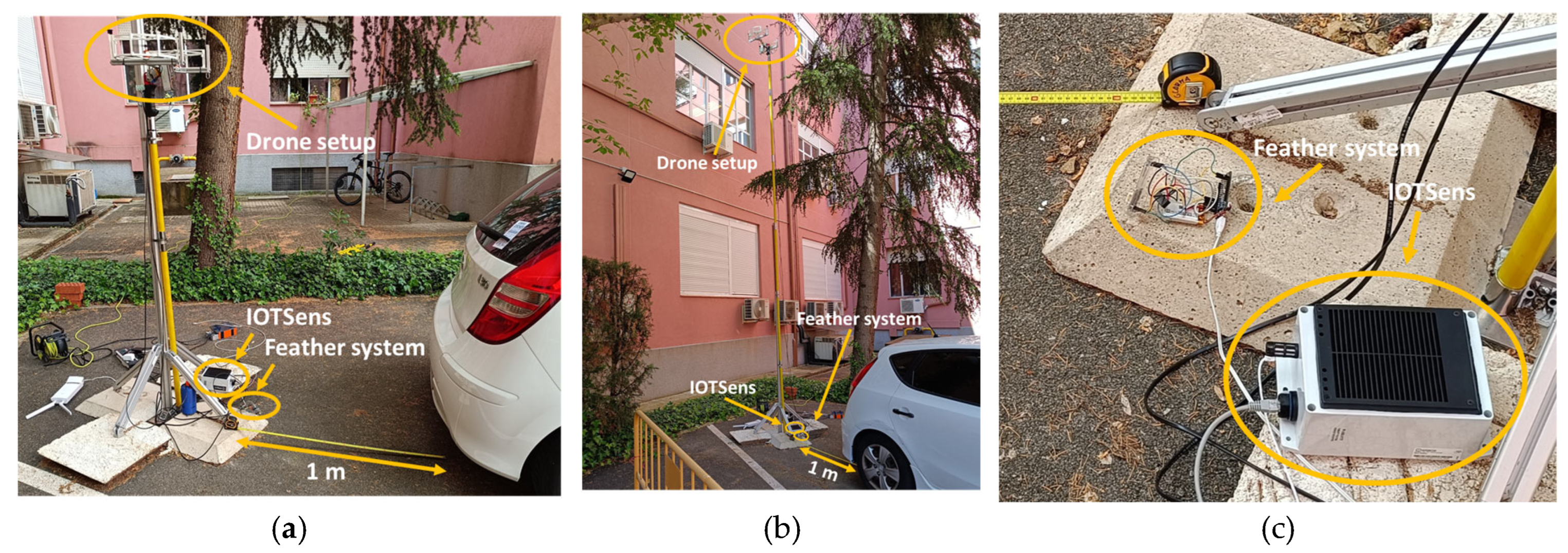
Figure 2.
Overview of the computational domain. (a) Side view illustrating the spacing between the inlet, the drone, and the back wall. (b) Drone height levels (H1–H6) and the geometry of the car’s rear surface, modeled as a fixed wall.
Figure 2.
Overview of the computational domain. (a) Side view illustrating the spacing between the inlet, the drone, and the back wall. (b) Drone height levels (H1–H6) and the geometry of the car’s rear surface, modeled as a fixed wall.
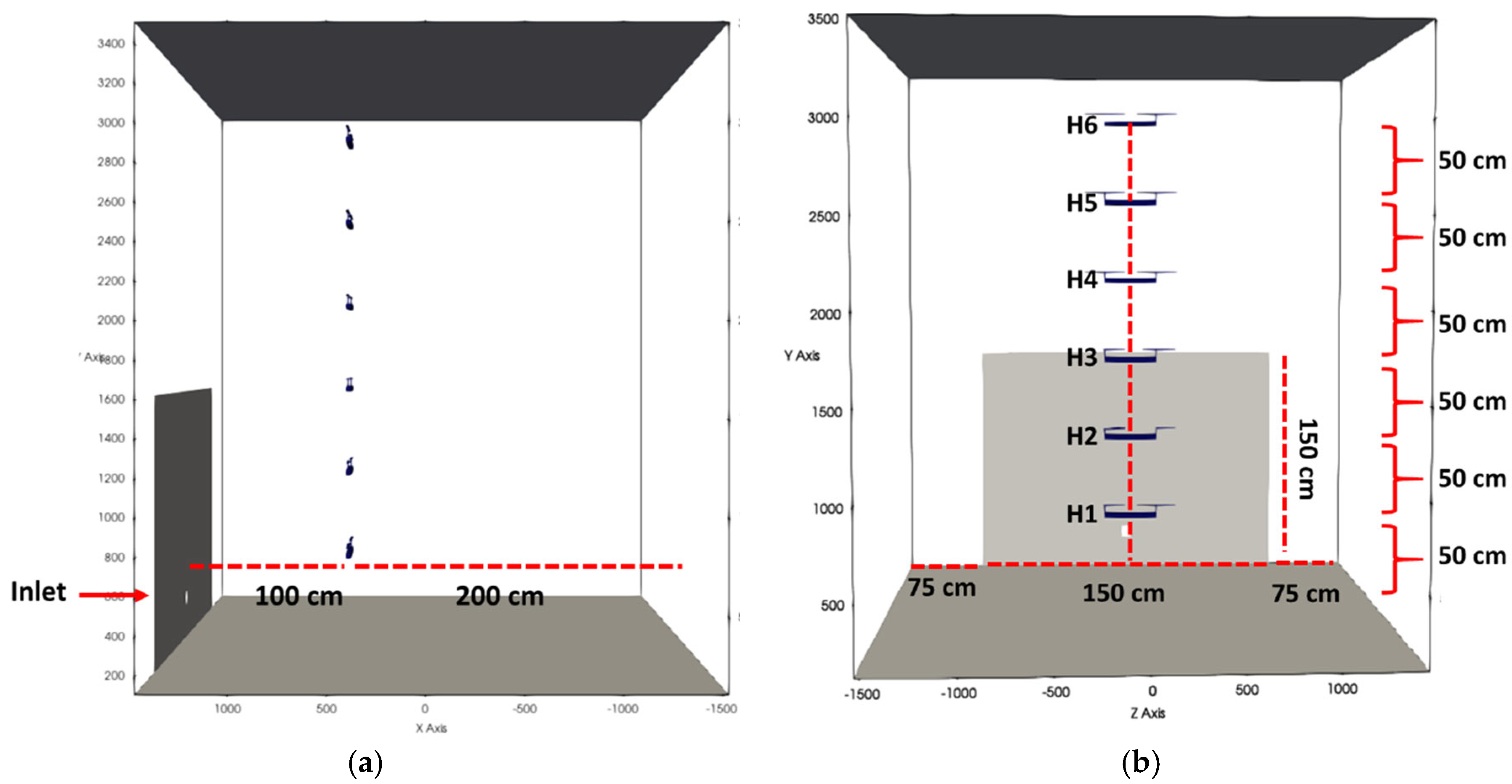
Figure 3.
Computational domain and applied boundary conditions, including exhaust inlet, MRF zones, open boundaries, and no-slip walls.
Figure 3.
Computational domain and applied boundary conditions, including exhaust inlet, MRF zones, open boundaries, and no-slip walls.
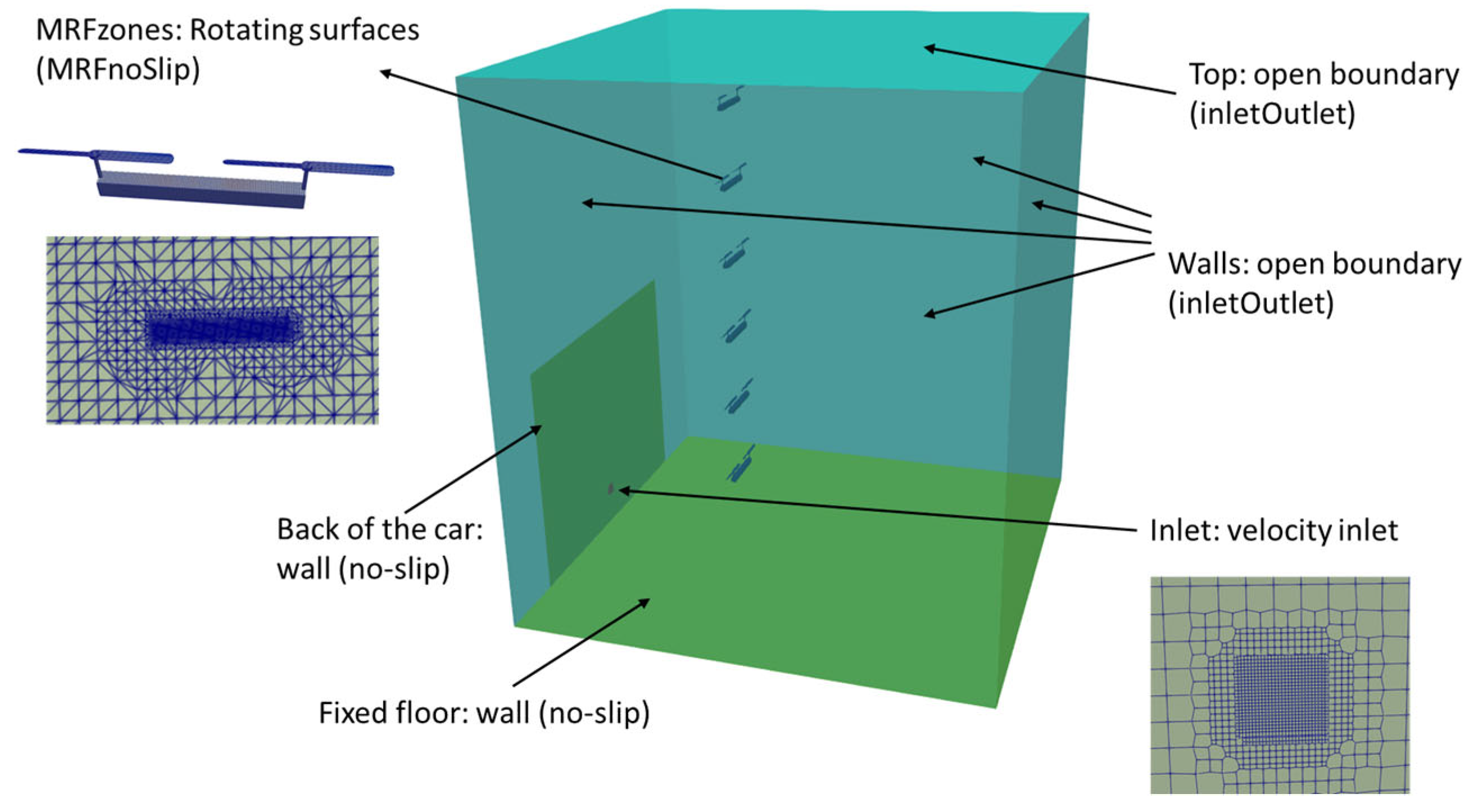
Figure 5.
Bottom right part of the meshes used for the independency study: (a) Base mesh, (b) Finex1, (c) Finerx2 and (d) Finerx3.
Figure 5.
Bottom right part of the meshes used for the independency study: (a) Base mesh, (b) Finex1, (c) Finerx2 and (d) Finerx3.
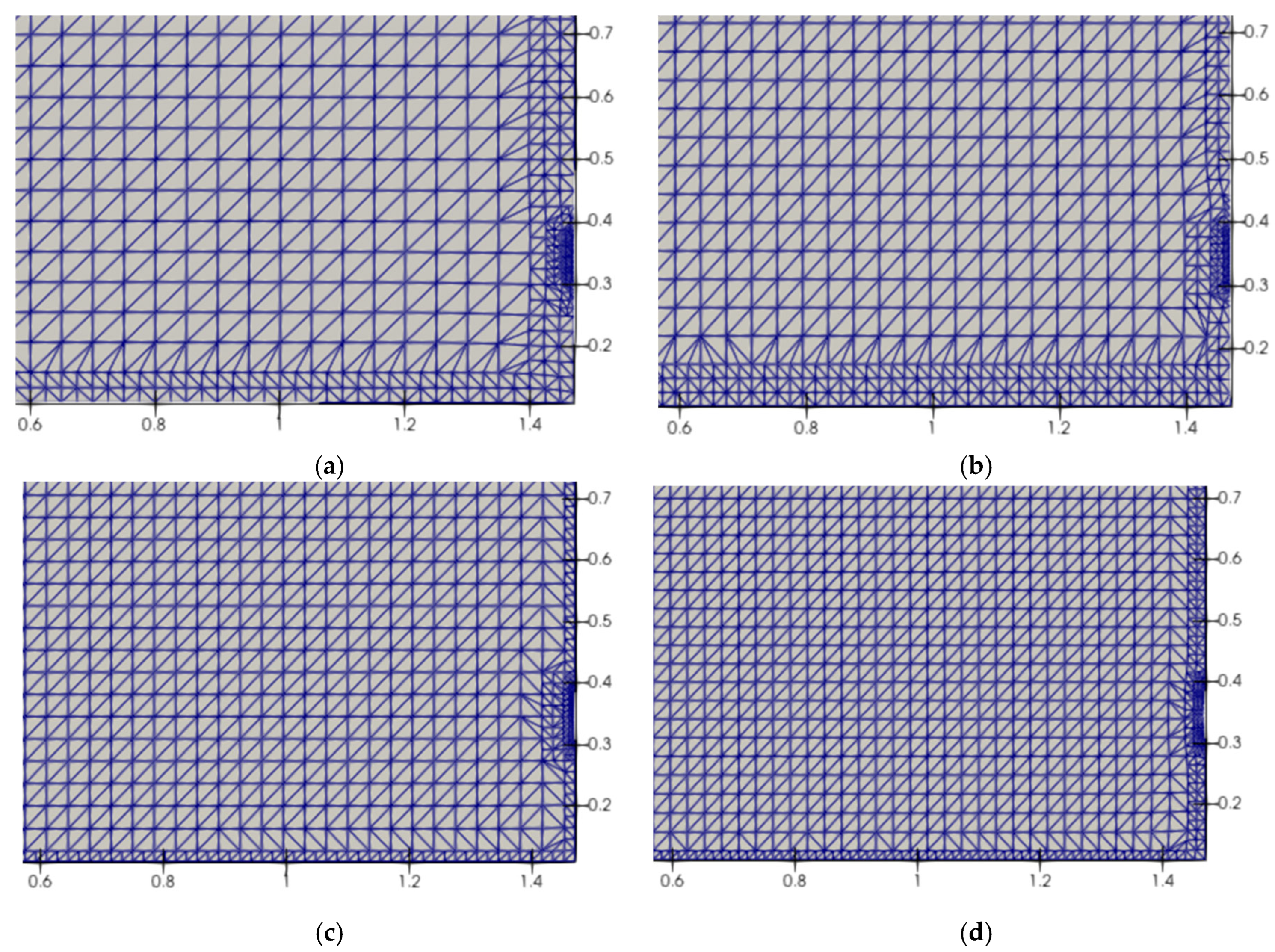
Figure 6.
Velocity magnitude profile used for the mesh independence analysis. The first velocity peak, highlighted by the dotted box, was selected as the comparison metric.
Figure 6.
Velocity magnitude profile used for the mesh independence analysis. The first velocity peak, highlighted by the dotted box, was selected as the comparison metric.
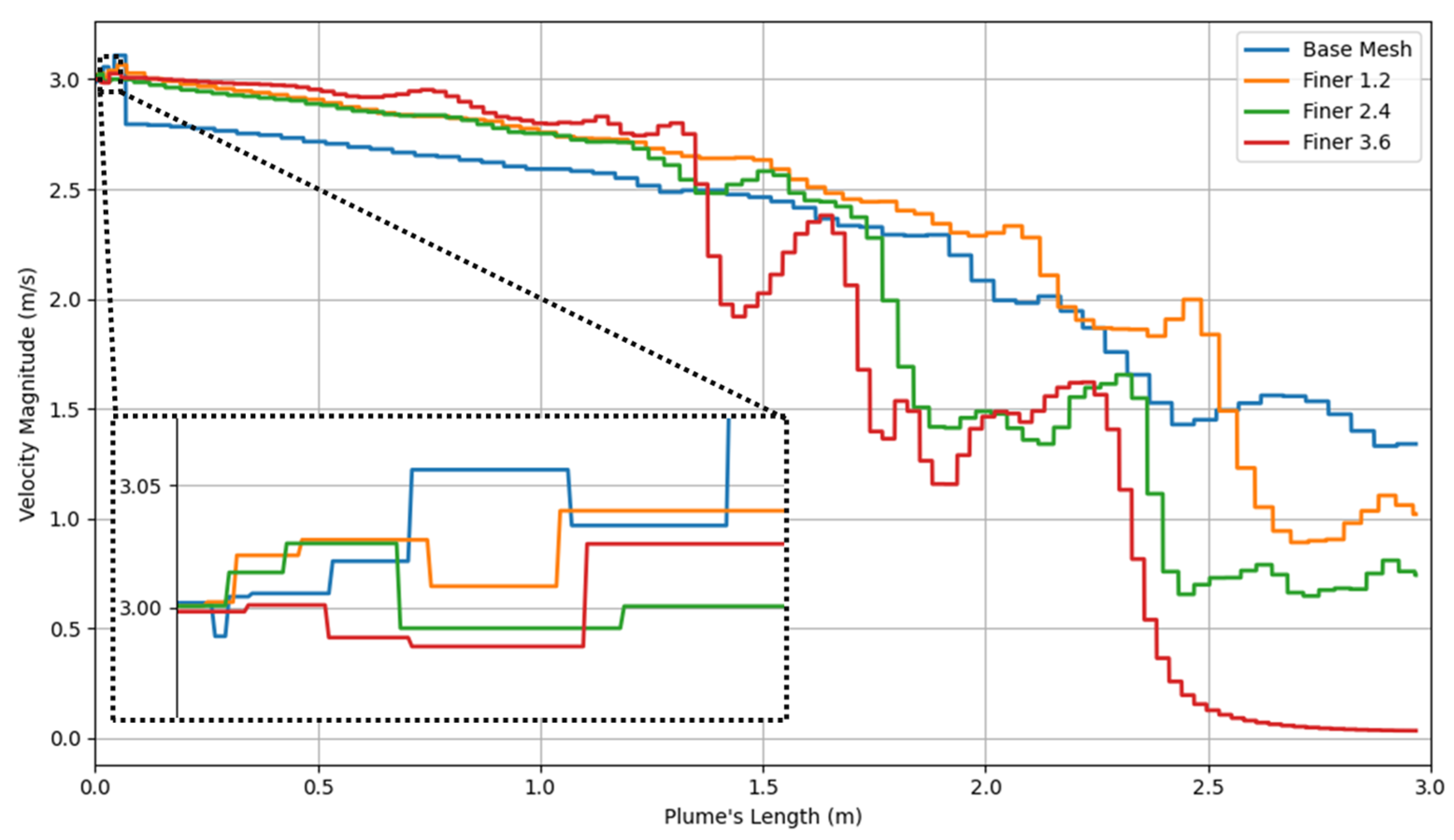
Figure 7.
Time-series of CO2 measurements obtained during the 8-hour experimental campaign at multiple heights and drone operating conditions. Legend format: Car_Drone_Height_Velocity.
Figure 7.
Time-series of CO2 measurements obtained during the 8-hour experimental campaign at multiple heights and drone operating conditions. Legend format: Car_Drone_Height_Velocity.
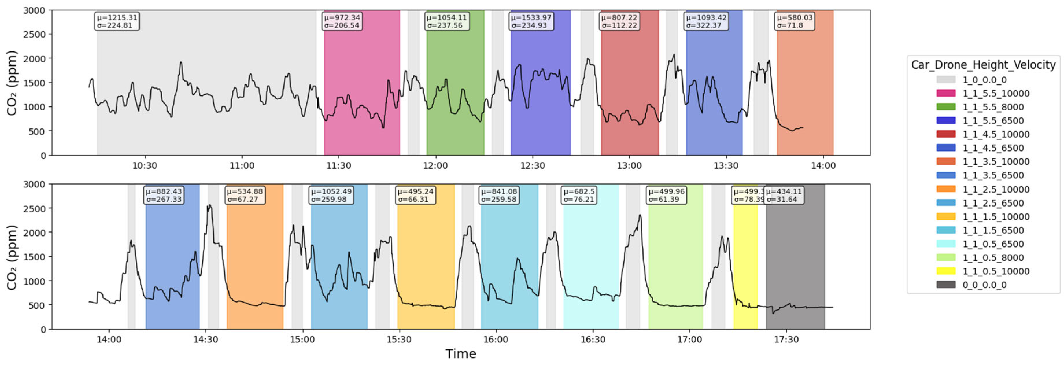
Figure 8.
Boxplots summarizing CO2 concentrations for all experimental configurations (Car_Drone_Height_Velocity).
Figure 8.
Boxplots summarizing CO2 concentrations for all experimental configurations (Car_Drone_Height_Velocity).
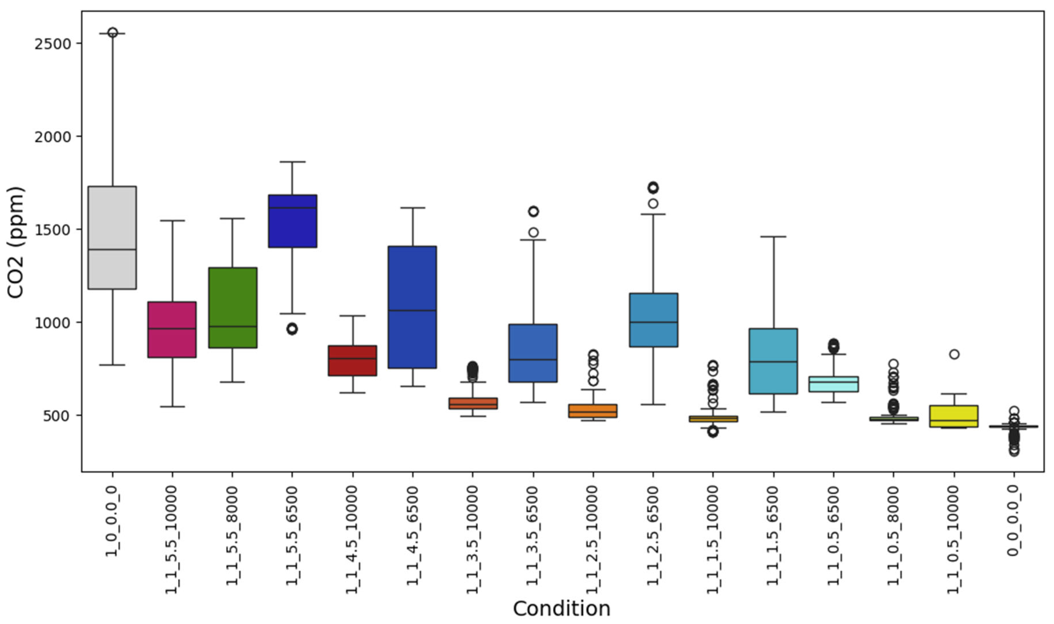
Figure 9.
CO2 plume development in first 5.5 s of simulation. All heights (H1-H6) compared without drone (ND).
Figure 9.
CO2 plume development in first 5.5 s of simulation. All heights (H1-H6) compared without drone (ND).
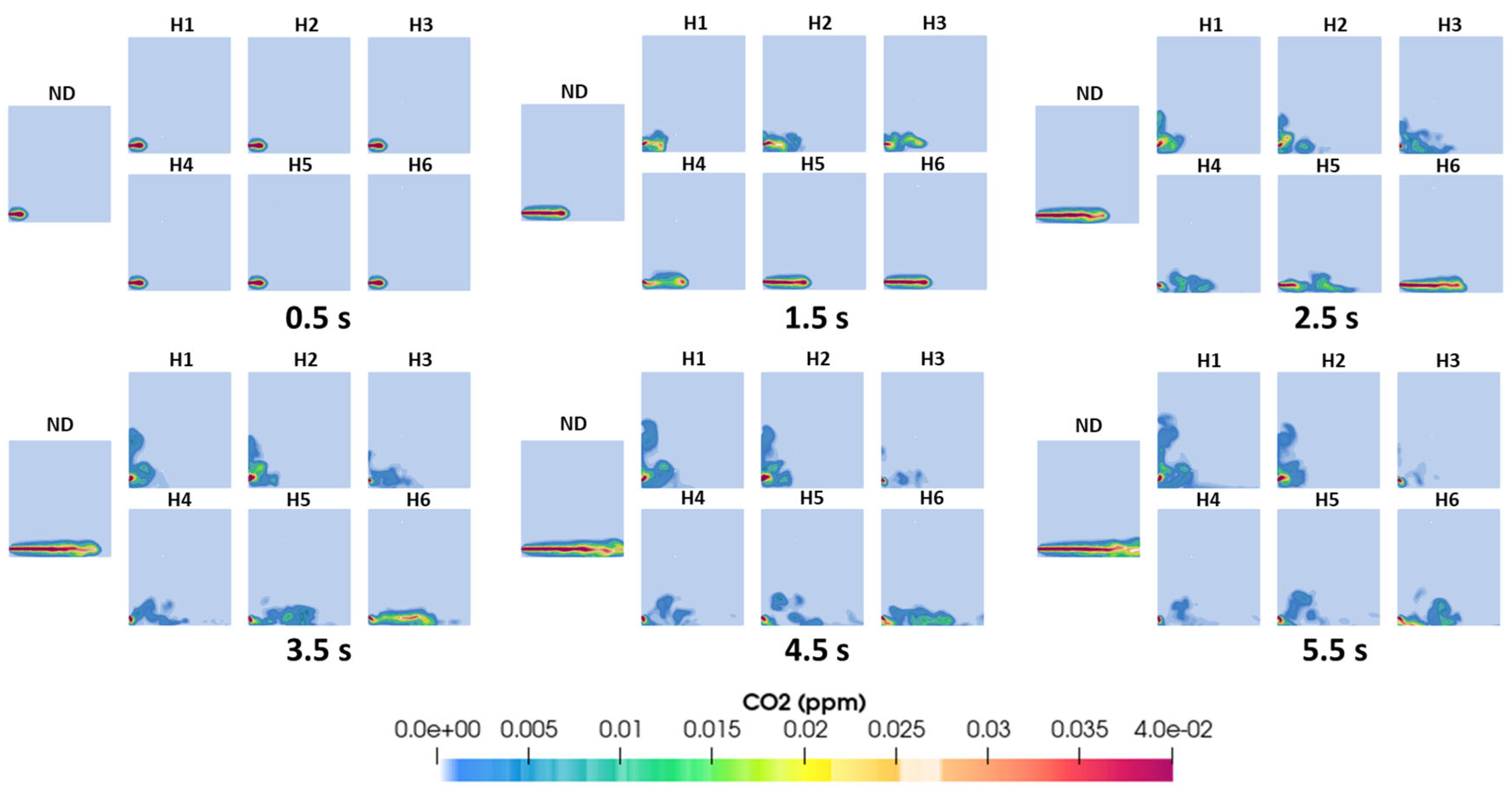
Figure 10.
CO2 concentration distribution in the computational domain after 25 s for all simulated UAV heights (H1–H6).
Figure 10.
CO2 concentration distribution in the computational domain after 25 s for all simulated UAV heights (H1–H6).
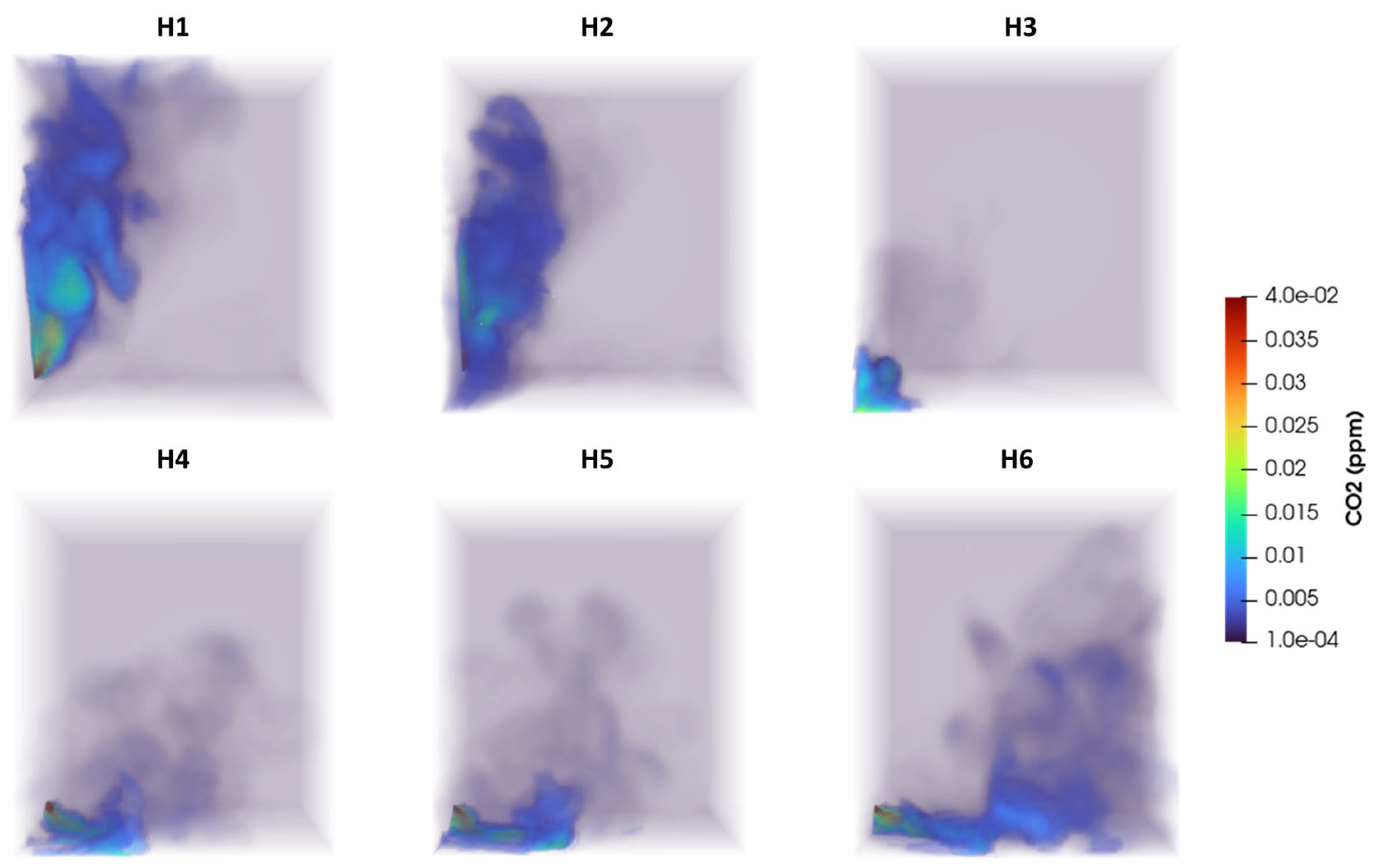
Figure 11.
Velocity magnitude during the transient evolution of the flow field at timesteps 0–5.5, 15, 20, and 25 s. All UAV heights (H1–H6) are compared with the no-drone (ND) reference case. Velocity is colored from 0 to 3 m/s (CO2 inlet velocity).
Figure 11.
Velocity magnitude during the transient evolution of the flow field at timesteps 0–5.5, 15, 20, and 25 s. All UAV heights (H1–H6) are compared with the no-drone (ND) reference case. Velocity is colored from 0 to 3 m/s (CO2 inlet velocity).
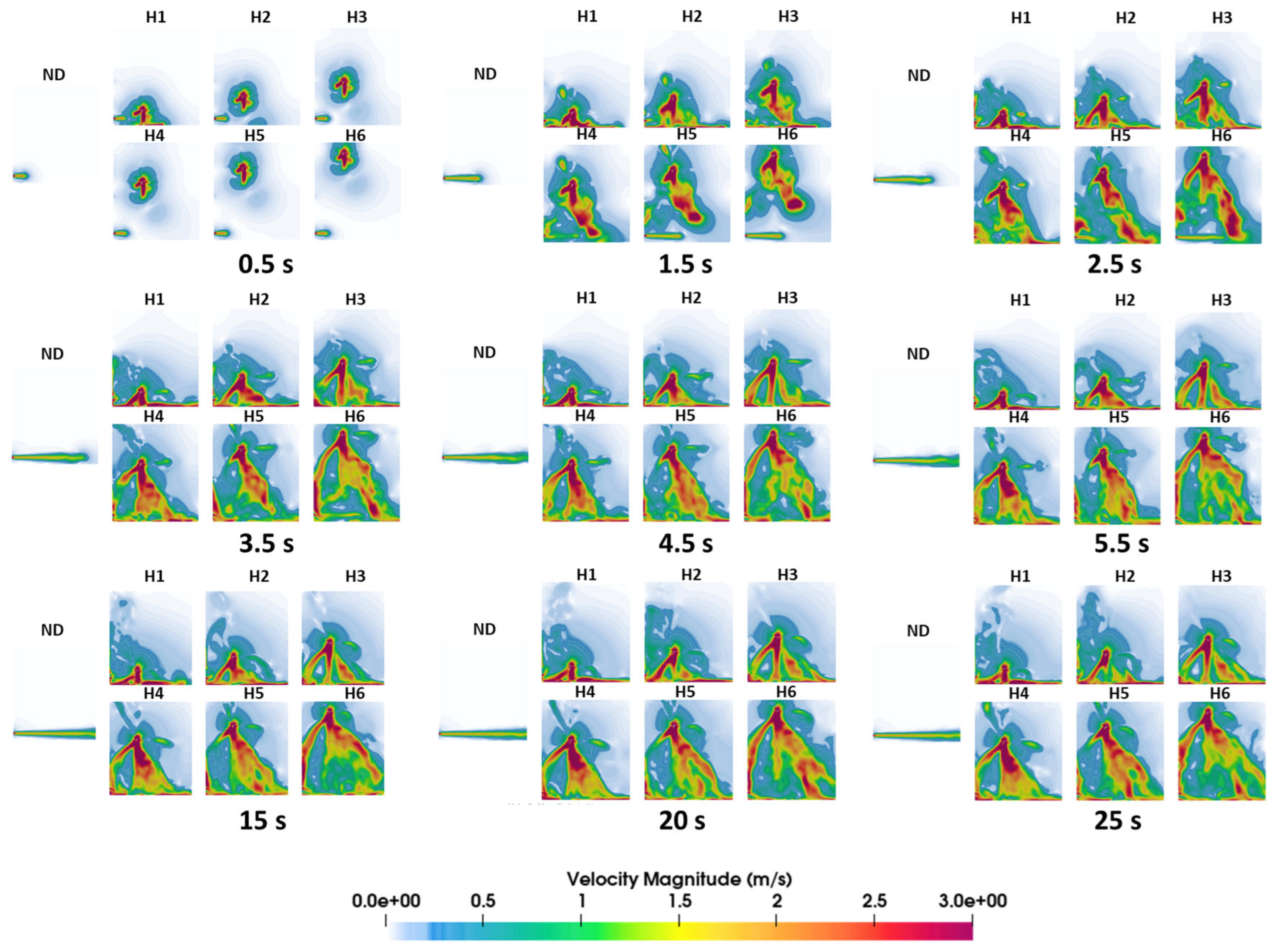
Figure 12.
Distribution of simulated CO2 concentrations at the probe location for different UAV heights.
Figure 12.
Distribution of simulated CO2 concentrations at the probe location for different UAV heights.
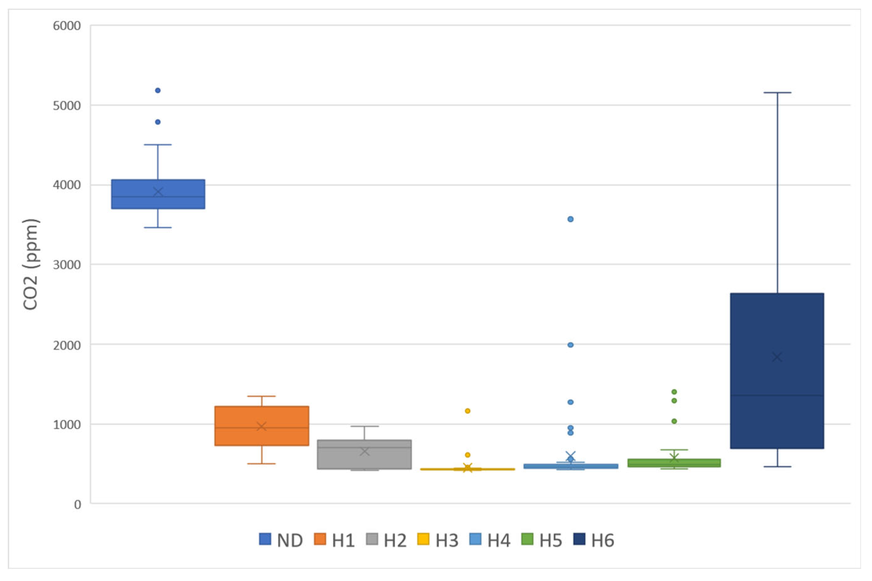

Table 1.
Experimental matrix.
| Rotor height (m) | Rotor speed (rpm) | Duration (min) |
|---|---|---|
| ND | 0 | 20 |
| 0.5 | 6500, 8000, 10000 | 20 |
| 1.5 | 6500, 10000 | 20 |
| 2.5 | 6500, 10000 | 20 |
| 3.5 | 6500, 10000 | 20 |
| 4.5 | 6500, 10000 | 20 |
| 5.5 | 6500, 8000, 10000 | 20 |
Table 2.
Boundary conditions applied in the simulations.
| Variable | Exhaust inlet | Open boundaries | Solid surfaces |
|---|---|---|---|
| Velocity (U) | Fixed value (−3,0,0) m s-1 |
inletOutlet | noSlip / MRFnoSlip |
| Pressure (p) | fixedFluxPressure | Fixed value (101.6 kPa) |
fixedFluxPressure |
| Temperature (T) | 324° K | inletOutlet (304° K) | zeroGradient |
| CO2 mass fraction | 0.08 | inletOutlet (0.00042) | zeroGradient |
| Air mass fraction | 0.92 | inletOutlet (0.99958) | zeroGradient |
| Turbulent kinetic energy (k) | 0.09 m2 s-2 | inletOutlet | kqRWallFunction |
| Turbulent viscosity (νt) | Calculated | Calculated | nutkWallFunction |
Table 3.
Mesh independency study.
| Mesh | Cell count | Maximum skewness | Air velocity magnitude (m/s) |
|---|---|---|---|
| 1 | 405,994 | 3.07 | 3.0189 |
| 2 | 655,029 | 1.25 | 3.0277 |
| 3 | 992,239 | 2.99 | 3.0262 |
| 4 | 1,710,536 | 2.08 | 3.0258 |
Table 4.
Final meshes used in the numerical campaign.
| Configuration | Cell number (x 103) |
Max. skewness | Max. Non-orthogonality |
|---|---|---|---|
| No MRF | 406 | 3.07 | 36.84 |
| H1 (0.5 m) | 457 | 3.59 | 64.89 |
| H2 (1.0 m) | 457 | 3.60 | 64.97 |
| H3 (1.5 m) | 457 | 3.56 | 64.84 |
| H4 (2.0 m) | 457 | 3.56 | 64.92 |
| H5 (2.5 m) | 457 | 3.56 | 64.91 |
| H6 (3.0 m) | 457 | 3.55 | 64.90 |
Table 5.
Comparison of CO2 concentrations measured by the two sensing platforms.
| System | Min (ppm) | Q1 (ppm) | Median (ppm) | Q3 (ppm) | Max (ppm) |
|---|---|---|---|---|---|
| IOTSENS | 427 | 450 | 506 | 783 | 1349 |
| Feather | 309 | 534 | 740 | 1012 | 1861 |
| Percentage Difference | -28% | +19% | +46% | +29% | +38% |
Table 6.
Simulated CO2 concentrations at the sensor location.
| Height (m) | CO2 concentration (ppm) | Reduction (%) |
|---|---|---|
| No drone | 3,659 | - |
| H1 | 904 | 75.20% |
| H2 | 665 | 81.80% |
| H3 | 506 | 88.53% |
| H4 | 612 | 83.26% |
| H5 | 670 | 85.36% |
| H6 | 1,816 | 50.37% |
Table 7.
Comparison Between Experimental and Numerical Results.
| Height (m) | Experimental reduction (%) | CFD Reduction (%) |
|---|---|---|
| 0.5 (H1) | 52.67% | 75.20% |
| 1.5 (H3) | 41.92% | 88.53% |
| 2.5 (H5) | 30.70% | 85.36% |
Disclaimer/Publisher’s Note: The statements, opinions and data contained in all publications are solely those of the individual author(s) and contributor(s) and not of MDPI and/or the editor(s). MDPI and/or the editor(s) disclaim responsibility for any injury to people or property resulting from any ideas, methods, instructions or products referred to in the content. |
© 2026 by the authors. Licensee MDPI, Basel, Switzerland. This article is an open access article distributed under the terms and conditions of the Creative Commons Attribution (CC BY) license (http://creativecommons.org/licenses/by/4.0/).
Copyright: This open access article is published under a Creative Commons CC BY 4.0 license, which permit the free download, distribution, and reuse, provided that the author and preprint are cited in any reuse.


