

Submitted:
13 July 2026
Posted:
16 July 2026
You are already at the latest version
Abstract
A current interest in lunar exploration led by Artemis program pushes scientists to search for lunar water deposits directly on the surface of the Moon with small robotic rovers. The Institute of Experimental and Applied Physics, Czech Technical University in Prague (IEAP CTU) is developing a miniature Timepix3-based detector Neutron HardPix capable of mapping the water deposits using non-invasive detection of neutrons created underground by cosmic rays and thermalized by hydrogen. This neutron spectrometer measures count rate variations of thermal, epithermal and fast neutrons attributed to the hydrogen abundance in lunar subsurface, while monitoring cosmic radiation as a natural source of neutrons. Neutron HardPix is based on the miniature (< 0.1 U, 130 g) radiation monitor HardPix with multiple space heritage.
Keywords:
neutron spectrometer
; Timepix
; HardPix
; hydrogen
; lunar water ice
; cosmic radiation
; albedo neutrons
1. Introduction
The hypothesis that water may exist as ice at the lunar poles was first advanced several decades ago [1,2]. Permanently shadowed regions (PSRs) near the lunar poles are characterized by extremely low temperatures, which are estimated to have remained below approximately 100 K for much of the Moon’s geological history, thereby providing conditions favorable for the long-term stability of water ice [3,4]. Subsequent lunar orbital investigations provided further indirect evidence supporting this hypothesis. Measurements from the bistatic radar experiment aboard NASA’s Clementine mission and from the neutron spectrometer onboard Lunar Prospector (Figure 1) indicated enhanced hydrogen concentrations in the polar regions, consistent with the presence of hydrogen-bearing volatiles such as water ice [5,6]. More recent observations from the Lunar Exploration Neutron Detector onboard NASA’s Lunar Reconnaissance Orbiter have reinforced the interpretation that significant quantities of water ice may be present within lunar PSRs [7,8,9].
In addition, orbital imaging and analyses of lunar samples suggest the presence of hydrogen-rich material in localized areas near the poles, potentially associated with water ice deposits. However, the spatial resolution of existing remote sensing remains insufficient to constrain the physical state, distribution, and concentration of these hydrogen-bearing materials. As a consequence, current knowledge of lunar water resources does not yet support reliable assessment or planning for resource extraction. These limitations underscore the necessity of future exploratory missions capable of conducting in-situ measurements at local scales to perform detailed hydrogen mapping and to directly characterize potential subsurface and surface volatile deposits.
1.1. Hydrogen Detection Using Neutrons
Neutron-based techniques have long been employed for the determination of moisture content in large volumes of geological materials. These methods exploit the strong interaction between neutrons and hydrogen, which is abundant in water molecules. Hydrogen is particularly effective at moderating fast neutrons through elastic scattering, thereby converting them into epithermal and ultimately thermal neutrons. Measurements of the resulting thermalized neutron flux therefore provide the fundamental observational basis for estimating the water or hydrogen content within a target material.
On the Moon, high-energy neutrons are continuously generated in the subsurface as a result of interactions between galactic cosmic rays (GCRs) and regolith nuclei. Once produced, these neutrons propagate through the lunar regolith, where they undergo multiple scattering events and may be removed from the neutron population through capture reactions. The presence of hydrogen in the subsurface significantly enhances neutron moderation efficiency.
1.2. Neutron Spectrometers
To date, the majority of flight-qualified neutron spectrometers have relied on 3He gas-filled proportional counters. Representative examples include the Dynamic Albedo of Neutrons (DAN) instrument onboard the Curiosity rover [10], the Neutron Spectrometer on Lunar Prospector [11] (Figure 1), the High Energy Neutron Detector (HEND) aboard Mars Odyssey [12], the Fine Resolution Epithermal Neutron Detector (FREND) onboard ESA’s Trace Gas Orbiter (TGO) [13], the Mercury Gamma-ray and Neutron Spectrometer (MGNS) on BepiColombo [14], and the Lunar Exploration Neutron Detector (LEND) aboard the Lunar Reconnaissance Orbiter [15].
Despite their proven scientific performance and extensive flight heritage, a significant fraction of the existing instruments has been developed by the Space Research Institute of the Russian Academy of Sciences (IKI), while many of the remaining non-Russian instruments originate from U.S. national laboratories, making them subject to export control regulations such as the International Traffic in Arms Regulations (ITAR). These factors complicate access to such technologies for international and commercial space missions. In addition, the integration of 3He gas proportional counters onto small spacecraft platforms presents non-negligible engineering challenges. These detectors operate with pressurized gas volumes and require high-voltage biasing for charge collection, both of which introduce potential risks in terms of mechanical safety, system reliability, and mission qualification.
In recent years, semiconductor detectors have gained increasing popularity in space applications owing to their compact size, low power consumption, and reduced cost. When coupled with an appropriate neutron conversion layer, such detectors can function effectively as neutron spectrometers. An example of this approach is the Lunar Lander Neutron and Dosimetry (LND) experiment aboard the Chang’E-4 lander [16].
1.3. HardPix Neutron Spectrometer
IEAP CTU has extensive experience in the development of silicon detectors optimized for the detection of both thermal and fast neutrons. The use of technologically advanced pixel detectors of the Timepix family, adapted for neutron detection through the application of suitable neutron conversion layers, has been proposed and systematically investigated in a number of publications. References [17,18,19] provide comprehensive information on these developments, including their deployment within the ATLAS experiment at the Large Hadron Collider (LHC) at CERN. These works also report on extensive experimental campaigns conducted at the Los Alamos Neutron Science Center (LANSCE), where detailed performance tests of the detectors were carried out under well-characterized neutron fields.
IEAP CTU, in collaboration with partner institutions, has also developed a number of radiation tracking instruments based on Timepix chips that have been successfully deployed in space applications. Timepix is a hybrid active pixel detector developed within the Medipix Collaboration at CERN. Its core component is a semiconductor sensor layer segmented into a matrix of 256 × 256 pixels with a pixel pitch of 55 µm, corresponding to an active area of approximately 1.4 × 1.4 cm². This sensor layer is bump-bonded to the readout application-specific integrated circuit (ASIC). The detector operates without the need for active cooling, relying solely on passive heat dissipation.
Timepix detectors can record detailed tracks of ionizing particles, corresponding to their trajectories within the solid-state pixel sensor. Track shapes can differ between particle types, energy, and angle, allowing discrimination of particle species, determination of incident direction, and measurement of ionization energy loss in the detector. By exploiting the Time-of-Arrival (ToA), three-dimensional track reconstruction can be achieved [20]. Particle identification is performed using a combination of track morphology and stopping-power information, enabling effective separation of electrons, protons, and heavier ions—particle species that are of primary relevance in the space radiation environment [21].
Since 2012, several of IEAP CTU miniature radiation monitors have been deployed aboard the International Space Station (ISS) in collaboration with the University of Houston and NASA [22,23,24]. A key milestone in demonstrating the suitability of Timepix technology for space applications was the Space Application of Timepix-based Radiation Monitor (SATRAM) project [25,26]. SATRAM operates as a remotely controlled spacecraft radiation monitor aboard the ESA Proba-V satellite, which has been in a near-polar Earth orbit at an altitude of approximately 820 km since its launch in May 2013.
Building on the heritage of the SATRAM project, several follow-up missions and developments were realized [27,28,29]. As a direct result of this accumulated experience with space radiation monitoring, IEAP CTU developed the HardPix detector (Figure 2), a next-generation radiation monitor based on the Timepix3 chip. HardPix incorporates onboard data processing and is designed as a versatile, universal radiation monitoring instrument for future space applications. The device has already acquired space heritage through its deployment aboard D-Orbit ION satellites launched in 2023 and 2025, as well as during the Heki ISS mission launched in 2025.
The HardPix instrument comprises two Timepix3 chipboards and an integrated data processing unit. The overall dimensions of the device are 81 × 40 × 22 mm³, with a total mass of approximately 130 g. The power consumption during measurement and onboard processing is typically in the range of 3–4 W.
IEAP CTU’s experience in developing Timepix-based neutron spectrometers, combined with the proven space heritage of the HardPix platform, has been consolidated into Neutron HardPix—a proposed neutron spectrometer for space missions, specifically targeted at mapping lunar water deposits aboard rovers, hoppers, and other surface or near-surface vehicles. This study addresses the suitability of Timepix3-based detectors as neutron spectrometers for use on the lunar surface. In the next phase, we will address the modification of the HardPix design for the actual mission.
2. Lunar Surface Neutron Count Rate Models
The essential task to assess the feasibility of Neutron HardPix for mapping lunar water deposits is modelling the expected neutron fluence rates in dependence on the water content of regolith. This modelling was performed by the Institute of Aerospace Medicine at the German Aerospace Center (DLR).
2.1. Models Used and Input Parameters/Assumptions
The radiation environment on the lunar surface caused by primary galactic cosmic radiation (GCR) was calculated for different fractions of water in the regolith with the PLANETOCOSMICS tool [30], which is an application to the Monte-Carlo framework Geant4 [31,32,33]. For the calculation Geant4 version 11.02 was used and the “Shielding” physics list was selected, which is recommended for applications for neutron transport (https://geant4-userdoc.web.cern.ch/UsersGuides/PhysicsListGuide/html/reference_PL/Shielding.html), in combination with the “EMZ” electromagnetic physics list option. Monte-Carlo calculations are a common tool to estimate the radiation environment from cosmic radiation on the lunar surface, e.g. [34] and references therein.
The primary radiation environment consisted of galactic cosmic radiation nuclei with charge number Z=1-28 (H to Ni) with energies between 10 MeV/nucleon and 200 GeV/nucleon as described by the DLR GCR model [35] for solar activity minimum and solar activity maximum conditions. The lunar surface was modelled as a box of regolith with a thickness of 50 m and a side length of 1000 km, the composition of the water-free regolith was taken from the elemental composition for Mare soils (Table 6.3 in [36]) and the corresponding amount of H and O was added for the different fractions of water (Table 1). The primary radiation source was a point source above the lunar surface with a cosine weighting in the zenith angle of the primary particles and the resulting particle flux was registered in the plane on top of the regolith. This setup is equivalent to an isotropic primary GCR flux and a point measurement on the lunar surface.
2.2. Calculated Spectra
The particles registered on top of the lunar regolith comprised protons, neutrons, photons, e-/e+, µ-/µ+, π-/π+, deuterons, tritons, 3He and nuclei from He to Fe. The calculations describe the response of the secondary neutron field as well as the background field of charged and uncharged particles. The calculated neutron spectra for different mass fractions of water (0%, 1%, 2%, 5%, 10% for solar minimum and 0%, 5%, and 10% for solar maximum) are illustrated in Figure 3 and numerical values of the thermal, epi-thermal and total neutron fluence rate are given in Table 2 (solar minimum) and Table 3 (solar maximum).
The calculated epi-thermal and total neutron fluence rates decrease monotonically with increasing water content; the epi-thermal neutron fluence is reduced by up to approximately 85% for both solar minimum and maximum for the maximum 10% H2O mass fraction, and the total neutron fluence by approximately 60%. The calculated thermal neutron fluence increases by approximately 20% for 1% H2O mass fraction and is also at an increased level at 2% H2O mass fraction. The thermal neutron fluence is reduced by about 30% (solar minimum) and 40% (solar maximum) for the maximum 10% H2O mass fraction. Between solar minimum and solar maximum, the neutron fluence decreases by 50% to 60%.
In order to estimate variations in the calculated neutron fluence rates caused by the selection of physics lists in Geant4, a number of physics lists were selected and the model calculations were re-run with otherwise unchanged setup (solar minimum case). The following additional physics lists were considered:
- QGSP_INCLXX_HP_EMZ
- FTFP_INCLXX_HP_EMZ
- FTFP_BERT_HP_EMZ
For the QGSP_INCLXX_HP_EMZ all five values for the water content were modelled, for the other two only the minimum (0% H2O) and maximum (10% H2O) were used. Table 4 (Appendix) contains the results for the fluence rate of thermal and epi-thermal neutrons and the total neutron fluence rate. The relative differences with respect to the previous physics list Shielding_EMZ are summarized in Table 5 (Appendix). The two physics lists using the INCLXX model in the intermediate energy range (20 MeV to 20 GeV) are very similar within a few percent and between 25% to 33% lower compared with Shielding_EMZ and FTFP_BERT_HP. It should be noted that the latter two both apply the BERT model for the intermediate energy range. The high precision (HP) model is part of all the listed physics lists for the neutron energy range below 20 MeV.
To investigate the expected variation of the neutron fluence rate for an alternative choice of regolith, a composition which is considered typical for lunar highlands was also applied (ferroan anorthosite, FAN, Table 6 in Appendix).
Using the FAN regolith composition, the neutron fluence rates were calculated with the Shielding_EMZ physics list for solar minimum conditions (Table 7). For low water content, the thermal neutron fluence is considerably higher (~70%) than previously calculated for the mare regolith. These differences disappear with increasing water content and are reduced to 2% for 10% water content. The epi-thermal neutron fluence is only slightly affected by the regolith composition and a few percent lower for the FAN regolith compared to the mare regolith.
In a layered setup, the impact of a potentially dry layer above the wet layer was investigated. The dry layer corresponded to 50 g/cm2 (~16.7 cm at a density of 3 g/cm3) FAN regolith on top of the wet layer of FAN regolith with either 5% or 10% water content. Using the layered geometry for 5% and 10% water content reduced the thermal neutron fluence by about 30% and 20% and increased the epi-thermal neutron fluence by about 40% and 60%, respectively (Table 7, Figure 4).
2.3. Comparison to Literature Data
The expected signal in the Lunar Prospector Neutron Spectrometer to varying amounts of water in the lunar regolith was estimated by [37,38,39]. Although most of their results include a detector response function and a transport function to the orbit and thus represent the detector count rate and not the thermal and epi-thermal neutron fluence on the lunar surface, a qualitative comparison can be made. For FAN regolith [38] calculated a maximum increase of 70% in thermal neutron counts with increasing water content up to a few percent and a steep decrease at higher values. A similar but less pronounced pattern shows in the calculations for the mare regolith (Table 2, Figure 4) with a maximum increase of about 20% at 1% water content. This pattern is, however, absent in the calculations for the FAN regolith (Table 7, Figure 4). The reason for this discrepancy is unknown but could be caused by different energy ranges or detector sensitivity and orbital transport function used by [38].
For epi-thermal count rates [38] calculated a monotonically decreasing count to about 70% of the initial count at 1% water content and about 20% of the initial count at 10% water. This is comparable to the results for FAN regolith (Table 7, Figure 4) which show a reduction to about 60% and 15% of the initial fluence rate at 1% and 10% water content, respectively.
[38] also presented in their Figure 1 differential neutron spectra on the lunar surface calculated for a number of regolith compositions. The peak neutron flux in the thermal energy range was between 5∙105 cm-2s-1MeV-1 and 5∙106 cm-2s-1MeV-1 at approximately 0.5∙10-7 MeV to 1∙10-7 MeV which is agreement with the results in Figure 3.
3. Neutron HardPix Converter Design
Semiconductor neutron detectors offer a compact solution for neutron detection and imaging applications. Owing to the absence of electric charge, neutrons cannot be detected directly through conventional ionization mechanisms; therefore, their detection in semiconductor devices generally relies on secondary effects. A common approach involves the deposition of neutron-reactive films onto semiconductor charged-particle detectors, where neutron capture reactions generate charged particles that can subsequently be detected.
3.1. Basic Concept of Thermal Neutron Detection
Among the neutron interactions most frequently exploited in thermal neutron detection are the 10B(n,α)7Li reaction and the 6Li(n,α)3H reaction (see [41] and the discussion therein). Thin-film neutron detectors typically consist of semiconductor detectors coated with one or more neutron-reactive conversion layers. Neutron absorption within the converter produces charged particles emitted in opposite directions, one of which may penetrate the semiconductor and deposit its energy, thereby enabling neutron detection.
3.2. Converter Material
The 10B(n,α)7Li reaction has a higher interaction probability than 6Li(n,α)3H for neutron energies below about 100 keV because of its larger absorption cross-section. However, the higher kinetic energies of the charged particles produced in the 6Li(n,α)3H reaction improve their detectability. This advantage is especially important in mixed-radiation environments, such as space, where neutron-induced events must be distinguished reliably from background. In Timepix detectors, 6Li(n,α)3H reaction products generate well-defined track signatures that support effective event discrimination. Therefore, 6Li-based conversion layers are considered particularly suitable for thermal and epithermal neutron detection in the Neutron HardPix instrument. While pure 6Li converters may provide thermal neutron detection efficiencies exceeding about 11% [41], their high chemical reactivity complicates fabrication and limits long-term stability. As a result, lithium fluoride (LiF), which is chemically more stable, is more commonly used in practice.
3.3. Converter Thickness
Neutron capture may take place at any position within the conversion layer. The charged reaction products generated in the neutron-reactive film lose part of their energy while traversing the converter material before they can reach the semiconductor sensor. This energy loss reduces the amount of energy ultimately deposited in the detector and thus affects the amplitude of the measurable signal.
The finite stopping power of the converter material sets a practical upper limit on the useful thickness of the conversion layer. Although a thicker layer increases the probability of neutron capture, this improvement is only beneficial up to the point at which the reaction products can still escape the converter and enter the semiconductor. Beyond that thickness, the charged particles are fully absorbed within the conversion layer and no longer contribute to detectable events. Additional increases in converter thickness therefore do not improve the detector response.
IEAP CTU has an extensive experience with LiF converter films applied to Timepix sensors [42,43,44] and used at Czech Metrology Institute (CMI), Los Alamos Neutron Science Center (LANSCE), ATLAS LHC and other facilities. However, we never had to worry about very low fluence rates, so the detection efficiency was not an issue, and we opted for very thin LiF layer of about 5-6 µm providing thermal neutron detection efficiency of around 1% (Figure 5).
McGregor et al. [41] claimed maximum efficiency of the LiF converter layer to be close to 4.5% using thickness of around 25 µm on a silicon diode. To confirm this efficiency with our pixelated sensor and perform a trade-off between detection efficiency and signal to noise ratio, we tested several thicknesses of LiF film and describe the results in the next chapter.
3.4. Epithermal Neutrons Conversion Layer
As discussed in the previous section, Li absorption cross section follows a 1/v dependence. Therefore, the energy dependent efficiency of the 6LiF decreases with energy as ε ∼ (see Figure 5). This means that LiF converter is sensitive to epithermal neutrons as well, though with significantly reduced efficiency compared to thermal neutrons. In order to precisely separate fluence rates of thermal and epithermal neutrons, and to assess whether Neutron HardPix can use also epithermal neutrons fluence rate to map water deposits, we included a cut-off filter in the form of Cadmium foil.
This is a similar method used by gas-proportional counters with two tubes like LEND where one tube is equipped with Cd foil which blocks thermal neutrons, making this tube sensitive to epithermal neutrons only. The second tube detects both thermal and epithermal energies. Thermal neutron fluence rate is then obtained by deducting the epithermal rate from the total one. We used an identical method and wrapped the thermal neutron setup in Cd foil to obtain epithermal neutron fluence rate and assess the feasibility of such solution for Neutron HardPix.
3.5. Fast Neutrons Conversion Layer
Fast neutrons conversion layer have a form of a thin (~1 mm) polyethylene (PE) layer in front of the Timepix3 sensor. Fast neutrons are detected by recoil protons created by fast neutrons interactions with the hydrogenous material.
Figure 6.
Example of the PE conversion mask on the Timepix detector.
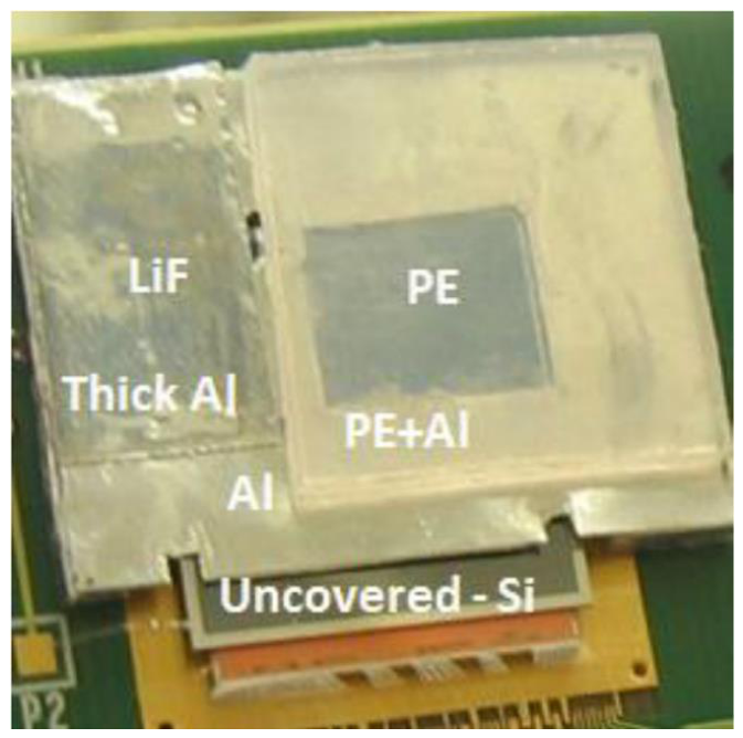
We experimented with PE converters for as long as with LiF, running a network of neutron detectors in the ATLAS LHC cavern and measuring at LANSCE facility where we obtained a peak detection efficiency for fast neutrons of 0.3 % at ~16 MeV (see Figure 5).
4. Neutron HardPix Breadboard Efficiency Measurements
4.1. Measurements Using AmBe Source at Van de Graaff Accelerator
The laboratory of the Van de Graaff (VdG) accelerator is devoted to basic and applied research in experimental nuclear physics. Besides serving as a source of light ions the facility serves namely as tuneable source of mono-energetic neutrons in relatively wide energy range (100 keV - 19 MeV).
Besides the accelerator, the facility is equipped with the Americium-Beryllium (AmBe) source producing a continuous spectrum of neutrons with energies in range ∼0.5–10 MeV. To slow down the neutrons, the AmBe source was inserted inside a hole in a polyethylene (PE) box with 8 cm of PE between the source and the Timepix3 detector (Figure 7). First, we made a comparison between four manufactured LiF layers of different thicknesses: 6.09 mg cm−2, 4.88 mg cm−2, 3.08 mg cm−2, and 1.44 mg cm−2, which correspond to approximately 6, 12, 18 and 24 µm. These LiF layers were spray-coated onto aluminium foils which are interchangeable so that an identical Timepix3 chipboard can be used for testing different layers.
Foils with LiF films have an area of 1x1 cm2 and cover half of the Timepix3 sensor area. An uncovered region (Si) is used for the background subtraction from high energy transfer particles leaving similar signatures in the sensor as conversion products. In this case, the background is given by the non-neutron field as well as neutron interactions in silicon, such as neutron elastic and inelastic scattering, 28Si(n,α)25Mg-reactions, 28Si(n,p)28Al reactions, more complex processes, and spallation reactions with thresholds 2.75 MeV, 4 MeV, and ≥20 MeV, respectively.
The lithium isotopic composition contained 96% of 6Li. The LiF layer was placed as close above the sensor as possible (Figure 7) so that the tritium and helium nuclei need to cross a minimum distance through the air. Although the exact neutron field was not known, it was the same for all 4 tested LiF layers, therefore allowing us to make a relative comparison.
Tritium and helium nuclei with energies in the order of ~2 MeV from the 6Li(n,α)3H reaction create clusters of shape called “heavy blob”1 in Timepix3 (Figure 8). The region under the area covered with LiF. The region of the sensor under LiF contains these heavy blobs as well as background heavy blobs and other ionizing particles. To remove background, we subtract heavy blobs in the control region without LiF and filter out particles (e.g. electrons, minimum ionizing particles), that create clusters of different shapes. Since the maximum detectable energy of the 6Li + n products is 2.73 MeV for the tritium nucleus, the deposited energy spectra of heavy blobs under LiF and in the control region have the same shape at higher energies. The spectra for the four different LiF layer thicknesses are shown in Figure 9.
The difference in spectra between different LiF converter thicknesses is clearly visible and demonstrates the effect of conversion products losing energy while traversing the converter layer itself, broadening the spectrum. While the thinnest layer has the lowest detection efficiency (as discussed later) it has a sharp peak in the energy spectrum which can be exploited in filtering the heavy blobs coming from the neutron conversion from the background with similar cluster shape.
By integrating the spectrum in energy, we get the total rate of tritium and helium nuclei giving us the relative detection efficiency of each layer. Figure 10 shows that the 4.88 mg cm−2 LiF layer was the most efficient of the four layers tested, achieving the rate of tritium and helium nuclei (8.85 ± 0.27) cm−2 s−1. The thicker layer has a similar rate which is in agreement with the McGregor [41] sensitivity curve where the rate enters a slowly declining plateau after an initial rise due to conversion products not penetrating the LiF layer from larger distances from the sensor.
The different rate of 4.88 mg cm−2 LiF layer between the first and second measurement was caused most probably by different proximity of the LiF converter layer to the sensor. Aluminium foils with different converter thicknesses were attached by hand and even a few microns of air gap difference will have a measurable effect on the remaining energy of tritons and alphas. Another difference from the idealistic models is the aluminium conductive layer on top of the Timepix3 chip needed for bias, which is discussed later.
After measuring that the 4.88 mg cm−2 thick LiF layer is the most efficient for neutron conversion, we decided to perform further experiments only with this layer. First, we tested the effect of cadmium shielding, which captures thermal neutrons but allows more energetic neutrons to pass.
Figure 11 shows a side view of a Timepix3 detector with cadmium metal sleeve wrapped around it. Although there were openings in the cadmium shielding, the excess of the cadmium shielding was ∼1 cm on both sides of the sensor with openings. Some thermal neutrons may have diffused through these openings and reached the LiF converter, but we consider this number negligible given the AmBe source was located in front of the sensor. Measured rate of heavy blobs with this shielding under the area with the LiF convertor was (0.633 ± 0.027) cm−2 s−1. We can compare this to the (8.85 ± 0.27) cm−2 s−1 rate from the previous measurement and calculate that after we subtract the epithermal neutrons rate behind Cadmium shield, the thermal neutrons accounted for (8.22 ± 0.27) cm−2 s−1 hits.
A small uncertainty comes from the fact that while most of the thermal neutrons came from the polyethylene box, some were thermalized elsewhere, for example in the wooden table on which the experiment sits. Some helium and tritium nuclei were possibly created directly by the fast neutrons (the cross section of 6Li + n → 3H + 4He reaction for fast neutrons is orders of magnitude smaller compared to slow neutrons, but non-zero).
Next, we performed measurements without the PE moderator to see the response in a field dominated by fast neutrons, which is a scenario expected on lunar surface. This gives us an upper estimate of how many heavy blobs in previous measurements were created by neutrons other than those moderated by the polyethylene box. The measured rates of heavy blobs were (0.111 ± 0.010) cm−2 s−1 under LiF and (0.028 ± 0.010) cm−2 s−1 under LiF covered with Cadmium shielding, which represent the systematic error of the thermal and epithermal neutron measurements with LiF converter.
This exercise represents the realistic scenario during the lunar rover mission where we can expect to detect not only thermal and epithermal neutrons moderated in the lunar regolith but also those moderated by the materials of the rover. This background can be mitigated by placing the detectors at the bottom of the spacecraft as close to the surface as possible though not entirely eliminated.
4.2. Calibration Using AmBe Source at the Czech Metrology Institute
Czech Metrology Institute (CMI) in Prague is equipped with the calibrated field of slow neutrons. It is created by inserting 6 AmBe sources in a graphite pile (Figure 12). Graphite serves as a moderator and in its centre the neutron field is close to isotropic with fluence rate (2.896 ± 0.035) × 104 cm−2 s−1, of which 92% neutrons are below 0.5 eV kinetic energy, i.e. thermal. The fluence rate is defined as the number of neutrons hitting a sphere divided by the cross-section area of the sphere. Therefore, the number of neutrons hitting a flat square area (such as the LiF converter) from all sides is half of the fluence rate (1.448 ± 0.018) × 104 cm−2 s−1.
Measurements with all 4 LiF layers of thicknesses 6.09 mg cm−2, 4.88 mg cm−2, 3.08 mg cm−2, and 1.44 mg cm−2 were repeated in this neutron field. Results are shown in Figure 13. The background at CMI was negligibly low. The most efficient convertor giving the highest heavy blobs count rate was the 6.09 mg cm−2 one with the rate of (397±4) cm−2 s−1. Within error bars, it was equalled by the 4.88 mg cm−2 converter with (389 ± 11) cm−2 s−1 heavy blobs under LiF. Dividing by the neutron fluence rate (1.448 ± 0.018) × 104 cm−2 s−1, we arrive at efficiency of detection (2.74 ± 0.04)% and (2.68 ± 0.08)% for the 6.09 mg cm−2 and 4.88 mg cm−2 converters, respectively. This is a calculation assuming a constant efficiency over all energies produced at CMI. We know that the efficiency depends on neutron kinetic energy as ε ∝ E−1/2, thus the peak efficiency for low energies of thermal neutrons will be slightly higher.
For 6.09 mg cm−2 and 4.88 mg cm−2 converters, we performed also measurements with the cadmium shielding. However, the rate of heavy blobs under the LiF converter was not uniform (see Figure 14). These were likely thermal neutrons diffusing through the side opening in the cadmium shielding (see Figure 11). We did not see such an effect in the measurements performed at VdG probably due to VdG source being placed in front of the sensor vs. the CMI neutron field being isotropic with thermal neutrons coming also from the sides.
This was the first reason why we were unable to reliably obtain detector efficiency for epithermal neutrons. The second was the fact that CMI doesn’t provide fluence rate for epithermal neutrons, only for thermal ones. And while they claim 92% of neutrons being thermal, the exact portion of epithermal ones in the remaining 8% is unknown. Nevertheless, we can estimate it using the LiF efficiency being directly proportional to Ek−1/2.
4.3. Fast Neutrons Calibration at LANSCE Facility
We performed measurements at VdG with the Timepix3 sensor and polyethylene converter which showed an excess of heavy blobs under the converter. However, given that we did not know the neutron field at VdG facility, and we had no other measurements to compare this relative measurement to, we rely on our previous measurement with Timepix3 at the Weapons Neutron Research (WNR) facility of the Los Alamos Neutron Science Center (LANSCE). The fast neutrons converter was a ∼1 mm thick polyethylene layer in front of the Timepix3 sensor serving the purpose of detecting recoil protons generated from fast neutron interactions with the hydrogen-rich material. Details of the setup at LANSCE are described in [42]
Neutron detection efficiency is shown as a function of the neutron energy in Figure 5. An increased response below the PE layer becomes visible above a neutron energy of 1 MeV. With increasing neutron energy, the range of recoil protons increases, so that the efficiently used thickness of the converter increases. At higher energy, however, the recoils receiving a large energy from the neutrons become penetrating, leaving only part of their energy in the silicon sensor until eventually, the energy is not enough to create the required neutron signature of a heavy blob or track. Thus, a maximal efficiency for detection of fast neutrons εmax = 0.3% was found at ∼16MeV.
4.4. Calibration Summary
We calibrated the Neutron HardPix detector at different facilities and obtained thermal neutron detection efficiency of 2.7 % average. While McGregor et al. [41] claims maximum efficiency close to 4.5 % in ideal scenario, there are some aspects of our measurement which will reduce the efficiency to values observed by us. The first is a small air gap between the Timepix3 sensor and the converter layer where Helium and tritium nuclei lose some of their energy reducing the number of conversion products which reach the sensor and deposit enough energy to be detected. This will of course not be an issue in the vacuum of space.
The second aspect is the 0.1 micron thick layer of aluminium on top of the Timepix3 sensor which serves as a conductor for distribution of the BIAS voltage across the sensor. It has the same effect as the air gap above, reducing the number of detected conversion products. Both issues can be in principle eliminated by applying the LiF converter layer directly on the sensor. LiF being conductive can perform as the BIAS conductor in place of Al, this option will be further investigated.
5. Acquisition Times Estimation
Lunar neutron fluxes simulated by DLR with Geant4 were used as input spectra. To improve our understanding of the lunar environment, we ordered the neutron fluence rates based on the physics lists and water percentages. Figure 15 shows the lethargy flux of neutrons from thermal to fast neutrons for different physics lists and water percentage. We observe that the shape of the neutron spectra is similar for all physics list used during the computation.
Considering that the shapes are similar for all physics lists (and thus the ratios between thermal, epithermal and fast neutrons) we tried to define the physics lists for the best and the worst-case scenario, representing the highest and lowest fluence rates respectively.
Next, we integrated the spectra of neutrons in 4 different ways: the entire spectra, the thermal neutron spectra, the epithermal neutron spectra and the fast neutron spectra, to compute, respectively, fluence rates of neutrons in total and in each energy band. Figure 16 shows the fluence rates of all, thermal, epithermal and fast neutrons based on the water content and on the physics list used.
We observe that the FTFP_BERT_HP_EMZ physics list gives the highest fluxes, but only slightly exceeding the results of the “Shielding” physics list, which is the recommended physics list for neutron transport. We use Shielding_EMZ as the best-case scenario since it has the second highest fluence rate. The QGSP_INCLXX_HP_EMZ physics lists gives the lowest fluence rates so it will represent the worst-case scenario.
It is important to note that fluence rates of the best-case scenario are at maximum 50 % higher than those of the worst case and physics list selection does not change fluence rate ratios between different energy bands, meaning that fluence rates of each physics list translate into acquisition times in a predictable way – higher fluence rate equals proportionally shorter acquisition times.
For the following calculations, we will be using the best-case scenario of Shielding_EMZ physics list.
5.1. Instrument Sensitivity Area and Detection Efficiency
Two units of Neutron HardPix detectors with two Timepix3 sensors each were used as input for detector surface area. One Timepix3 sensor (2 cm2) was used for detection of thermal neutrons, one for epithermal neutrons, one for fast neutrons, and one as a reference of the charged particles environment and to subtract the background. Figure 17 shows the neutrons detection efficiencies according to the energy, efficiencies measured in the previous section are shown as full curves, while efficiencies simulated using detector response functions are shown as markers with the associated Monte Carlo uncertainties.
The simulated LiF layer is sensitive to thermal and epithermal neutrons with an efficiency very similar to the measured efficiency. The LiF layer with Cd shielding is sensitive to epithermal neutrons but blocks the thermal ones. It also shows a small reaction to fast neutrons at very high energies (>50 MeV). Finally, the simulated PE conversion layer is sensitive to fast neutrons with a slightly lower efficiency than the measured one.
Flux of fast neutrons does not change as radically with hydrogen abundance as the flux of thermal and epithermal neutrons, but we use it to overcome the behaviour of thermal neutron flux which increases at first with rising hydrogen abundance and then decreases with higher abundance making it difficult to distinguish between 0 and 3-5% water ratio using just thermal neutron flux alone. Based on the flux of cosmic ray albedo neutrons calculated for the lunar surface, we estimated the number of neutrons detected by two Neutron HardPix units’ sensors. Based on the counts and ratio of thermal, epithermal and fast neutrons measured in a given time, we can estimate the relative change in the water ratio in the local lunar regolith.
5.2. Estimated Count Rates
5.3. Estimated Acquisition Times
Based on the count rates estimated in Figure 18 we estimated the time needed to predict the water content using with a surface area of 2 cm2 for each energy bin as described above. This estimation is presented in Figure 19 for 0, 1, 2, 5 and 10 % water mass ratio at 3σ. It shows that it should be possible to differentiate 5% water mass ratio change, i.e. between the 0% and 5%, and between 5% and 10%, in roughly 20 minutes. Detecting 3% difference between 2% and 5% water mass ratio takes around 50 minutes, while detecting 2% difference between 0% and 2% takes roughly 80 minutes. Detecting low difference of 1% between 0% and 1%, or 1% and 2% then takes in the order of several (>2) hours, nicely representing increasing acquisition times needed to detect smaller changes in lunar regolith water mass ratio. However, these calculations were made just considering the number of neutrons detected not their weight in the prediction nor the ratio in between them.
6. Neutron HardPix Hydrogen Detection Measurements
6.1. Phantom Materials and Setup
Possible materials for lunar regolith simulants available at VdG facility included pure silica sand SiO2 in 25L barrels and PE sheets. The goal of these simulants was to recreate neutron radiation environment on lunar surface above regolith with different water mass ratios as closely as possible. The best setups were designed based on simulations of the effects of simulants on VdG monoenergetic neutron field. During these simulations limitations of the VdG possibilities became apparent.
- In order to simulate thermal and epithermal neutron field within the VdG chamber, we had to use the lowest practical beam settings, i.e. 1 MeV neutrons. Moderating enough fast neutrons in higher settings to simulate thermal and epithermal spectra shape representative of lunar surface would require large amounts of material, mainly sand, which would be difficult within the timeframe of this project.
- To properly model the fast neutron part of lunar spectra, we would need neutrons of energies of at least 10 MeV, ideally up to 1 GeV, though from simulations it seems that neutrons from 10 MeV to 1 GeV are not influenced by hydrogen so 10 MeV might be enough. For this reason, fast neutron count rates were not used in the analysis of VdG measurements with Neutron HardPix breadboard (BB) even though we did measure them.
- Simulations showed that spectra representative of very low water mass ratios (~0-1%) are very difficult to simulate with the setup available at VdG and thus these were not tested, which is unfortunate as the difference in count rates between the dry regolith and small water mass ratios promised to be much larger than between different water mass ratios and it would have been very interesting to experimentally validate this.
6.2. Experimental Setup
Two HDPE barrels with dimensions of 28 x 28 x 15 cm3 and filled with SiO2 with density of 1.5 g/cm3 were placed in the neutron beam and followed by PE sheets with dimensions of 32 x 32 x 1 cm3 with density of 0.960 g/cm3 (Figure 20). Measurements were performed with total PE thickness of 2, 3, 4 and 5 cm, where HDPE barrels add an extra 2 mm per each wall thickness, i.e. 8 mm of PE total.
Detectors were placed behind these simulants. Neutron HardPix BB with LiF converter layer was used for thermal+epithermal neutrons detection. The same detector was later covered with 1 mm Cd foil to block thermal neutrons and measure epithermal neutron count rate. Two detectors with PE converter from the MICADO project (https://www.utef.cvut.cz/micado_en) were used to detect fast neutrons, though as stated above, these measurements were not used in the end as the count rate of fast neutrons in the VdG lowest settings was not high enough for a meaningful analysis.
The following experimental setups were modelled and measured at VdG neutron beam, all using 1 MeV neutrons as a source. The neutron spectra calculated for the lunar surface were normalized to the expected neutron flux at the accelerator at 0.05 eV to facilitate the comparison of the shape of the spectra:
Figure 21.
Neutron spectra calculated for the VdG accelerator setup (cyan) compared to the results of the model for the lunar surface with dry FAN regolith (black) and H2O contents in legends (blue). VdG spectra were calculated for simulants with 30 cm SiO2 + 2.8 cm PE (upper left), 30 cm SiO2 + 3.8 cm PE (upper right) and 30 cm SiO2 + 4.8 cm PE (lower left).
Figure 21.
Neutron spectra calculated for the VdG accelerator setup (cyan) compared to the results of the model for the lunar surface with dry FAN regolith (black) and H2O contents in legends (blue). VdG spectra were calculated for simulants with 30 cm SiO2 + 2.8 cm PE (upper left), 30 cm SiO2 + 3.8 cm PE (upper right) and 30 cm SiO2 + 4.8 cm PE (lower left).
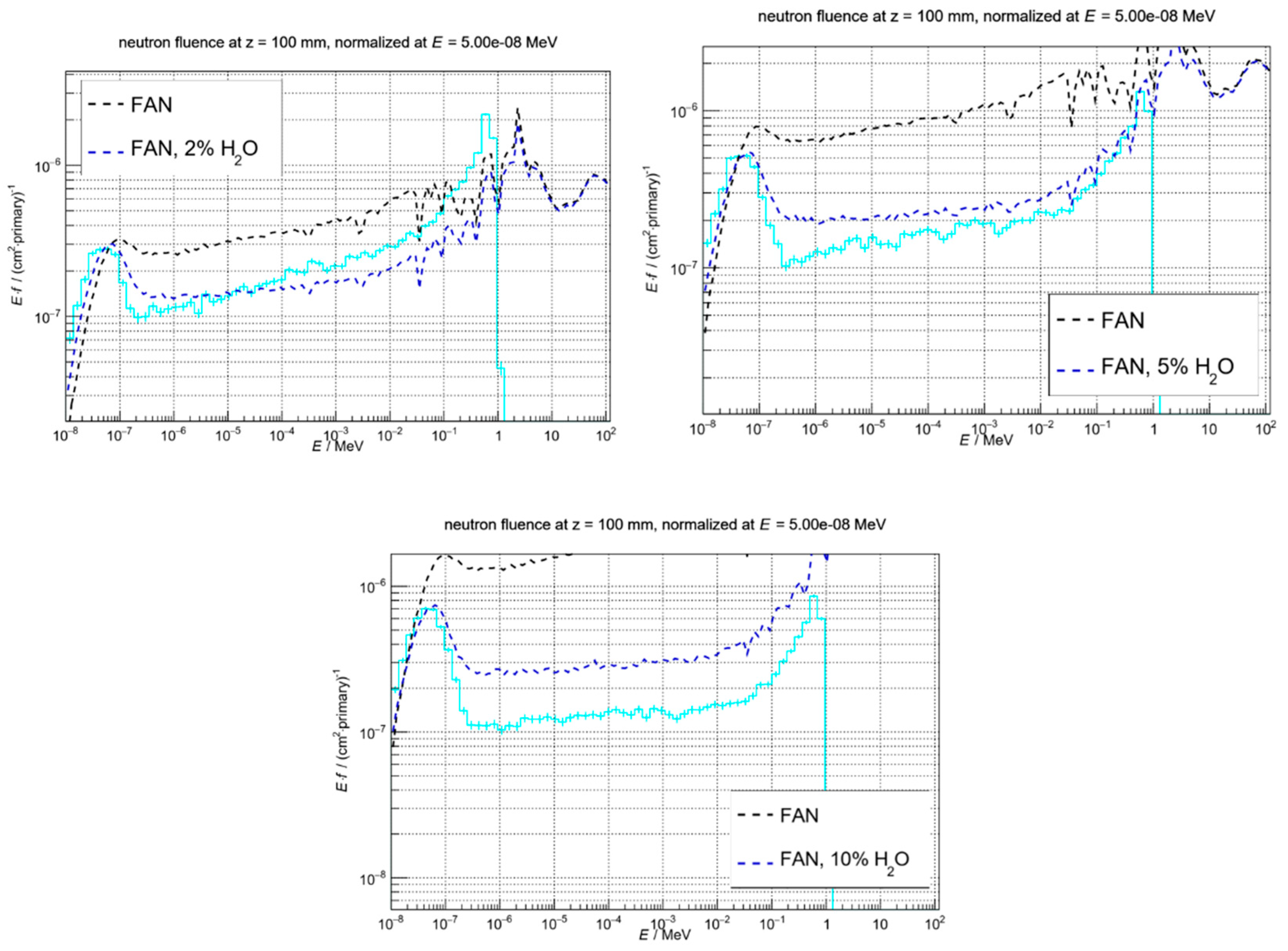
The measurements were done with 1-hour cycles and then normalized with respect to the dose measured by Berthold LB6411 neutron counter/dosemeter. The result of measurement is summarized in Figure 22, showing measured count rates representing water mass ratios compared to simulations of VdG spectra. These measurements are in good agreement with simulations, some differences could be explained by the thermal background from walls and surrounding material increasing with larger amounts of PE.
While we were unable to precisely reproduce neutron spectra on top of the lunar regolith at our VdG facility, produced neutron environments were sufficiently similar to verify the performance of tested neutron spectrometers in thermal and epithermal neutron regions. Differences were caused mainly by the low quantity of material to sufficiently thermalize fast neutrons, forcing us to use the lowest setting for VdG, but also backscattering as well as idealistic modelling of the VdG source. Despite these approximations, Neutron HardPix breadboard measurements showed very good agreement with simulations, validating its performance as a neutron spectrometer in the environment expected on the lunar surface. Next steps will include repeating such verification with a mechanically representative prototypes of a multilayer Neutron HardPix to validate the setup described above.
7. Conclusions
Secondary cosmic ray neutron spectra on the lunar surface on top of the regolith were calculated with Geant4 and the dependence of thermal, epithermal and fast neutron fluence rates on the regolith water content was estimated for different physics lists, solar cycle phases and layered regolith scenarios. These calculations show that the fluence rate change between dry and wet regolith is much more pronounced than those between different mass ratios of hydrogen, implying that searching for any water ice in an otherwise dry regolith will be easier and quicker than searching for water content fluctuations. They also show strong influence of GCR flux on the resulting neutron field, demonstrating the significance of a radiation monitor for a lunar mission.
Neutron converters for semiconductor detectors were presented and their detection efficiency simulated and verified by measurements at calibrated neutron facilities. While efficiencies are relatively low, the advantages of using COTS sensor with LiF and PE converter layers are the availability of these components, our long-term experience using them in mixed neutron environments and no gamma-ray background since the converter products are very specific and easily recognizable in a mixed radiation field. There should be no problem in modifying this solution for space application with the exception of the Cadmium shield, which has problems with outgassing and whiskers. However, we are currently exploring options of using Gadolinium instead.
Estimated count rates expected on lunar surface show that for dry regolith the best option would be dedicating one sensor for each neutron energy bin plus one “naked” sensor for reference and neutron background subtraction. The easiest baseline from the engineering standpoint would thus be 2 HardPix units with 2 sensors each. For low water mass ratios between 1-5% the change of epithermal neutron fluence rate is higher than the change of fast neutron fluence rate but this effect is reversed for higher mass ratios >5% where epithermal neutron fluence rate is already minimal and hardly detectable. Unless the water content at the landing site of the mission is known, the safe option would be to measure all neutron energies.
Acquisition times for the neutron spectrometer setup described above was calculated and showed duration in the order of ~1 hour to detect fluctuations of neutron count rates representing water mass ratio change of 2-3% in the range between 0 and 10%. While these times favor missions with longer still periods like hoppers, they are sufficiently low even for fast rovers. In these cases, high precision measurements can be performed during charging stops and measurement during roving can provide maps of hydrogen distribution with <1 km resolution, significantly improving maps obtained by orbital probes.
Funding
The development of HardPix was carried out under a programme of, and funded by, the European Space Agency Contract No. 4000135884/21/NL/CRS. Study of Neutron HardPix scientific performance was carried out under a programme of, and funded by, the European Space Agency Purchase Order No. 5001039803. CTU team acknowledges support by a grant from the Programme Johannes Amos Comenius under the Ministry of Education, Youth and Sports of the Czech Republic [CZ.02.01.01/00/22_008/0004590].
Acknowledgments
Authors acknowledge support of VdG and CMI facilities staff.
Appendix

Table 4.
Absolute values of the neutron fluence rates on the lunar surface from primary GCR calculated for solar minimum conditions and different water content in the regolith and Geant4 with different physics lists.
Table 4.
Absolute values of the neutron fluence rates on the lunar surface from primary GCR calculated for solar minimum conditions and different water content in the regolith and Geant4 with different physics lists.
| Solar minimum | ||||||
| E < 0.48 eV | 0.48 eV ≤ E < 0.1 MeV | total | ||||
| f / (cm2∙s)-1 | uncertainty | f / (cm2∙s)-1 | uncertainty | f / (cm2∙s)-1 | uncertainty | |
| H2O mass fraction | Geant4 physics list: Shielding_EMZ | |||||
| 0.00 | 0.409 | 0.002 | 4.410 | 0.008 | 10.977 | 0.014 |
| 0.01 | 0.490 | 0.002 | 2.615 | 0.006 | 8.719 | 0.011 |
| 0.02 | 0.476 | 0.002 | 1.907 | 0.004 | 7.582 | 0.010 |
| 0.05 | 0.376 | 0.002 | 1.125 | 0.003 | 5.931 | 0.008 |
| 0.10 | 0.270 | 0.001 | 0.697 | 0.002 | 4.709 | 0.007 |
| H2O mass fraction | Geant4 physics list: QGSP_INCLXX_HP_EMZ | |||||
| 0.00 | 0.276 | 0.002 | 3.007 | 0.006 | 7.823 | 0.010 |
| 0.01 | 0.337 | 0.002 | 1.799 | 0.004 | 6.319 | 0.009 |
| 0.02 | 0.328 | 0.002 | 1.334 | 0.003 | 5.551 | 0.008 |
| 0.05 | 0.267 | 0.001 | 0.799 | 0.002 | 4.386 | 0.006 |
| 0.10 | 0.194 | 0.001 | 0.499 | 0.002 | 3.514 | 0.005 |
| H2O mass fraction | Geant4 physics list: FTFP_INCLXX_HP_EMZ | |||||
| 0.00 | 0.281 | 0.002 | 3.054 | 0.008 | 7.968 | 0.014 |
| 0.10 | 0.193 | 0.001 | 0.504 | 0.002 | 3.554 | 0.007 |
| H2O mass fraction | Geant4 physics list: FTFP_BERT_HP_EMZ | |||||
| 0.00 | 0.414 | 0.002 | 4.494 | 0.008 | 11.226 | 0.014 |
| 0.10 | 0.275 | 0.001 | 0.716 | 0.002 | 4.833 | 0.006 |
Table 5.
Relative differences of the neutron fluence rates on the lunar surface from primary GCR calculated for solar minimum conditions and different water content in the regolith and Geant4 for different physics lists with respect to Shielding_EMZ.
Table 5.
Relative differences of the neutron fluence rates on the lunar surface from primary GCR calculated for solar minimum conditions and different water content in the regolith and Geant4 for different physics lists with respect to Shielding_EMZ.
| Solar minimum | |||
| E < 0.48 eV | 0.48 eV ≤ E < 0.1 MeV | total | |
| % difference wrt. Shielding_EMZ | % difference wrt. Shielding_EMZ | % difference wrt. Shielding_EMZ | |
| H2O mass fraction | Geant4 physics list: QGSP_INCLXX_HP_EMZ | ||
| 0.00 | -32.5 | -31.8 | -28.7 |
| 0.01 | -31.2 | -31.2 | -27.5 |
| 0.02 | -31.1 | -30.0 | -26.8 |
| 0.05 | -28.8 | -29.0 | -26.1 |
| 0.10 | -28.3 | -28.3 | -25.4 |
| H2O mass fraction | Geant4 physics list: FTFP_INCLXX_HP_EMZ | ||
| 0.00 | -31.3 | -30.7 | -27.4 |
| 0.10 | -28.5 | -27.6 | -24.5 |
| H2O mass fraction | Geant4 physics list: FTFP_BERT_HP_EMZ | ||
| 0.00 | 1.5 | 1.9 | 2.3 |
| 0.10 | 1.7 | 2.8 | 2.6 |
Table 6.
Elemental mass fractions used in the model calculations for the different water content. The first line represents the FAN regolith without water [38,40].
| Elemental mass fraction in FAN regolith | |||||||||
| H2O mass fraction | H | O | Na | Mg | Al | Si | Ca | Ti | Fe |
| 0.00 | 0.0000 | 0.4560 | 0.0045 | 0.0051 | 0.1763 | 0.2066 | 0.1359 | 0.0008 | 0.0148 |
| 0.01 | 0.0011 | 0.4603 | 0.0045 | 0.0050 | 0.1745 | 0.2045 | 0.1345 | 0.0008 | 0.0147 |
| 0.02 | 0.0022 | 0.4646 | 0.0044 | 0.0050 | 0.1728 | 0.2025 | 0.1332 | 0.0008 | 0.0145 |
| 0.05 | 0.0056 | 0.4776 | 0.0043 | 0.0048 | 0.1675 | 0.1963 | 0.1291 | 0.0008 | 0.0141 |
| 0.10 | 0.0112 | 0.4992 | 0.0041 | 0.0046 | 0.1587 | 0.1859 | 0.1223 | 0.0007 | 0.0133 |
| 1 |
A "heavy blob" cluster satisfies all of these conditions:
|
References
- Watson, K.; Murray, B.C.; Brown, H. On the possible presence of ice on the Moon. J. Geophys. Res. 1961, 66, 3033–3045. [Google Scholar] [CrossRef]
- J. Arnold, J. Ice in the lunar polar regions. Geophys. Res. 1979, 84(B10), 5659–5668. [Google Scholar] [CrossRef]
- Lucey, P. Elements 2009, 5, 41–46. [CrossRef]
- M., Anand, Lunar Water: A Brief Review. Earth Moon Plan. 2010, 107, 65–73. [CrossRef]
- Nozette, S.; Lichtenberg, C. L.; Spudis, P.; Bonner, R.; Ort, W.; Malaret, E.; Robinson, M.; Shoemaker, E. M. The Clementine bistatic radar experiment. Science 1996, 274(5292), 1495–1498. [Google Scholar] [CrossRef] [PubMed]
- Feldman, W. C.; Maurice, S.; Binder, A. B.; Barraclough, B. L.; Elphic, R. C.; Lawrence, D. J. Fluxes of Fast and Epithermal Neutrons from Lunar Prospector: Evidence for Water Ice at the Lunar Poles. Science 1998, vol. 281, 1496. [Google Scholar] [CrossRef]
- Colaprete, A.; Schultz, P.; Heldmann, J.; Wooden, D.; Shirley, M.; Ennico, K.; Hermalyn, B.; Marshall, W.; Ricco, A.; Elphic, R. C.; Goldstein, D.; Summy, D.; Bart, G. D.; Asphaug, E.; Korycansky, D.; Landis, D.; Sollitt, L. Detection of water in the LCROSS ejecta plume. Science 2010, 330(6003), 463–468. [Google Scholar] [CrossRef] [PubMed]
- Spudis, P. D.; et al. Evidence for water ice on the Moon: Results for anomalous polar craters from the LRO Mini-RF imaging radar. J. Geophys. Res. Plan. 2013, 118, 2016–2029. [Google Scholar] [CrossRef]
- Hayne, P. O.; et al. Evidence for exposed water ice in the Moon’s south polar regions from Lunar Reconnaissance Orbiter ultraviolet albedo and temperature measurements. Icarus 2015, 255, 58–69. [Google Scholar] [CrossRef]
- Mitrofanov, I.G.; Litvak, M.L.; Varenikov, A.B.; et al. Dynamic Albedo of Neutrons (DAN) Experiment Onboard NASA’s Mars Science Laboratory. Space Sci. Rev. 2012, 170, 559–582. [Google Scholar] [CrossRef]
- Feldman, W.C.; Barraclough, B.L.; Fuller, K.R.; Lawrence, D.J.; Maurice, S.; Miller, M.C.; Prettyman, T.H.; Binder, A.B. The Lunar Prospector gamma-ray and neutron spectrometers. Nuclear Instruments and Methods in Physics Research Section A: Accelerators, Spectrometers, Detectors and Associated Equipment 1999, Volume 422, Issues 1–3. [Google Scholar]
- Hurley, K.; Mitrofanov, I.; Kozyrev, A.; Litvak, Maxim; Grinkov, A.; Charyshnikov, S.; Boynton, William; Fellows, Chuck; Harshman, K.; Hamara, Dave; Shinohara, Christopher; Starr, R.; Cline. Mars Odyssey Joins The Third Interplanetary Network. Astrophys. J. Suppl. Ser. 2008, 164, 124. [Google Scholar] [CrossRef] [PubMed]
- Mitrofanov, I.; Malakhov, A.; Golovin, D.; Litvak, M.; Sanin, A.; Semkova, J. “FREND experiment on ESA's TGO mission: science tasks, initial space data and expected results”. 2017, 14685. [Google Scholar]
- Mitrofanov, I.G.; Kozyrev, A.S.; Konovalov, A.; Litvak, M.L.; Malakhov, A.A.; Mokrousov, M.I.; Sanin, A.B.; Tret’ykov, V.I.; Vostrukhin, A.V.; Bobrovnitskij, Yu.I.; Tomilina, T.M.; Gurvits, L.; Owens, A. The Mercury Gamma and Neutron Spectrometer (MGNS) on board the Planetary Orbiter of the BepiColombo mission. In Planetary and Space Science; 2010; Volume 58, pp. Issues 1–2. [Google Scholar]
- Mitrofanov, I.; Sanin, A.; Golovin, D.D.; Litvak, Maxim; Konovalov, A.A.; Kozyrev, A.; Malakhov, A.V.; Mokrousov, M.; Tretyakov, V.; Troshin, V.; Uvarov, V.; Varenikov, A.B.; Vostrukhin, A.A.; Shevchenko, V.; Valery, Shvetsov; Krylov, A.R.; Timoshenko, Gennady; Bobrovnitsky, Y.I.; Tomilina, T.; Evans, Larry. Experiment LEND of the NASA Lunar Reconnaissance Orbiter for High-Resolution Mapping of Neutron Emission of the Moon. Astrobiology 2008, 8, 793–804. [Google Scholar] [CrossRef] [PubMed]
- Wimmer-Schweingruber, R.; Yu, Jia; Böttcher, Stephan; Zhang, Shenyi; Burmeister, Soenke; Lohf, Henning; Guo, Jingnan; Xu, Zigong; Schuster, Björn; Seimetz, Lars; von Forstner, Johan; Ravanbakhsh, Ali; Knierim, Violetta; Kolbe, Stefan; Woyciechowsky, Hauke; Kulkarni, S.; Yuan, Bin; Shen, Guohong; Wang, Chunqing; Fu, Qiang. The Lunar Lander Neutron and Dosimetry (LND) Experiment on Chang'E 4. 2020. [Google Scholar] [CrossRef]
- Bergmann, B.; Caicedo, I.; Leroy, C.; Pospisil, S.; Vykydal, Z. ATLAS-TPX: a two-layer pixel detector setup for neutron detection and radiation field characterization. J. Instrum. 2016, 11, P10002. [Google Scholar] [CrossRef]
- Burian, P.; Broulim, P.; Bergmann, B.; Georgiev, V.; Pospisil, S.; Pusman, L.; Zich, J. Timepix3 detector network at ATLAS experiment. J. Instrum. 13, C11024 2018. [CrossRef]
- Bergmann, B.; Nelson, R.O.; O'Donnell, J.M.; Pospisil, S.; Solc, J.; Takai, H.; Vykydal, Z. Time-of-flight measurement of fast neutrons with Timepix detectors. J. Instrum. 2014, 9, C05048. [Google Scholar] [CrossRef]
- Bergmann, B.; Pichotka, M.; Pospisil, S.; et al. 3D track reconstruction capability of a silicon hybrid active pixel detector. Eur. Phys. J. C 2017, 77, 421. [Google Scholar] [CrossRef]
- Gohl, Stefan; Bergmann, Benedikt; Evans, Hugh; Nieminen, Petteri; Owens, Alan; Pospisil, Stanislav. Study of the radiation fields in LEO with the Space Application of Timepix Radiation Monitor (SATRAM). Adv. Space Res. 2018. [Google Scholar] [CrossRef]
- Kroupa, M.; et al. A semiconductor radiation imaging pixel detector for space radiation dosimetry. In Life Sciences in Space Research; 2015; Volume 6, pp. 69–78. [Google Scholar]
- Stoffle, N.; et al. Timepix-based radiation environment monitor measurements aboard the International Space Station. Nucl. Instrum. Methods Phys. Res. Sect. A Accel. Spectrom. Detect. Assoc. Equip. 2015, 782, 143–148. [Google Scholar] [CrossRef]
- Turecek, D.; Pinsky, L.; Jakubek, J.; Vykydal, Z.; Stoffle, N.; Pospisil, S. Small Dosimeter based on Timepix device for International Space Station, 2011, December. J. Instrum. 6, C12037. [CrossRef]
- Granja, C.; Polansky, S.; Vykydal, Z.; Pospisil, S.; Owens, A.; Kozacek, Z.; Mellab, K.; Simcak, M. The SATRAM Timepix spacecraft payload in open space on board the Proba-V satellite for wide range radiation monitoring in LEO orbit. Planet. SPACE Sci. 2016, Volume: 125, Pages: 114–129. [Google Scholar]
- Gohl, St.; Bergmann, B.; Granja, C.; Owens, A.; Pichotka, M.; Polansky, S.; Pospisil, S. Measurement of particle directions in low earth orbit with a Timepix. J. Instrum. 2016, 11, C11023. [Google Scholar] [CrossRef]
- Filgas, R. Space radiation monitoring with Timepix. Astron. Nachr. 2018, 339, 386–390. [Google Scholar] [CrossRef]
- Filgas, R.; Malich, M.; Kuwahara, T.; et al. RISEPix—A Timepix-based radiation monitor telescope onboard the RISESAT satellite. Astron. Nachr. 2019, 340, 674–680. [Google Scholar] [CrossRef]
- Wu, X.; Ambrosi, G.; Azzarello, P.; et al. "Penetrating particle ANalyzer (PAN). Adv. SPACE Res. 2019, Volume: 63(Issue: 8), Pages: 2672–2682. [Google Scholar]
- Desorgher, L.; Flückiger, E. O.; Gurtner, M. The PLANETOCOSMICS Geant4 application. 36th COSPAR Sci. Assem. 2006, 36, 2361–2361. [Google Scholar]
- Agostinelli, S.; Allison, J.; Amako, K.; Apostolakis, J.; Araujo, H.; Arce, P.; et al. GEANT4-a simulation toolkit. Nuclear Instruments & Methods in Physics Research Section a-Accelerators Spectrometers Detectors and Associated Equipment 2003, 506(3), 250–303. [Google Scholar] [CrossRef]
- Allison, J.; Amako, K.; Apostolakis, J.; Araujo, H.; Dubois, P. A.; Asai, M.; et al. Geant4 developments and applications. IEEE Trans. Nucl. Sci. 2006, 53, 270–278. [Google Scholar] [CrossRef]
- Allison, J.; Amako, K.; Apostolakis, J.; Arce, P.; Asai, M.; Aso, T.; et al. Recent developments in GEANT4. Nuclear Instruments & Methods in Physics Research Section a-Accelerators Spectrometers Detectors and Associated Equipment 2016, 835, 186–225. [Google Scholar] [CrossRef]
- Matthiä, D.; Berger, T. Radiation exposure and shielding effectson the lunar surface. Space Weather 2024, 22, e2024SW004095. [Google Scholar] [CrossRef]
- Matthiä, D.; Berger, T.; Mrigakshi, A. I.; Reitz, G. A ready-to-use galactic cosmic ray model. Adv. Space Res. 2013, 51, 329–338. [Google Scholar] [CrossRef]
- Lindsay, J. F. Lunar stratigraphy and sedimentology; Elsevier, 1976. [Google Scholar]
- Feldman, W. C.; Maurice, S.; Binder, A. B.; Barraclough, B. L.; Elphic, R. C.; Lawrence, D. J. Fluxes of Fast and Epithermal Neutrons from Lunar Prospector: Evidence for Water Ice at the Lunar Poles. Science 1998, 281(5382), 1496–1500. [Google Scholar] [CrossRef] [PubMed]
- Lawrence, D. J.; Feldman, W. C.; Elphic, R. C.; Hagerty, J. J.; Maurice, S.; McKinney, G. W.; Prettyman, T. H. Improved modeling of Lunar Prospector neutron spectrometer data: Implications for hydrogen deposits at the lunar poles. J. Geophys. Res. Plan. 2006, 111(E8). [Google Scholar] [CrossRef]
- Lawrence, D. J.; Peplowski, P. N.; Wilson, J. T.; Elphic, R. C. Global Hydrogen Abundances on the Lunar Surface. J. Geophys. Res. Plan. 2022, 127(7), e2022JE007197. [Google Scholar] [CrossRef]
- Haskin, L.; Warren, P. Lunar Chemistry. In Lunar Sourcebook, A User's Guide to the Moon; Heiken, G. H., Vaniman, D. T., French, B. M., Eds.; 1991; pp. 357–474. [Google Scholar]
- McGregor, D.S.; Hammig, M.D.; Yang, Y.-H.; Gersch, H.K.; Klann, R.T. Design considerations for thin film coated semiconductor thermal neutron detectors—I: basics regarding alpha particle emitting neutron reactive films. Nuclear Instruments and Methods in Physics Research Section A: Accelerators, Spectrometers, Detectors and Associated Equipment 2003, Volume 500(Issues 1–3), Pages 272–308. [Google Scholar] [CrossRef]
- Smolyanskiy, P.; et al. A two-layer Timepix3 stack for improved charged particle tracking and radiation field decomposition. 2024 JINST 19 C02016. [Google Scholar] [CrossRef]
- Biskup, Bartolomej; Bergmann, Benedikt; Broulim, Pavel; Burian, Petr; Malich, Milan; Manek, Petr; Meduna, Lukas; Mora, Yesid; Pichotka, Martin; Pusman, Lukas; Rubovic, Peter; Slavicek, Tomas; Smolyanskiy, Petr. EPJ Web Conf. 253 07010; Timepix3 detector network for nuclear waste monitoring. 2021. [CrossRef]
- Rubovič, Peter; Ekendahl, Daniela; Vykydal, Zdeněk; Hůlka, Jiří; Bergmann, Benedikt; Pospíšil, Stanislav; Štekl, Ivan. Dosimetry in mixed neutron-gamma fields with a Timepix detector. Radiat. Meas. Vol. 2018, Volume 119, Pages 22–26. [Google Scholar] [CrossRef]
Figure 1.
The dark blue and purple areas at the Moon's poles indicate neutron emissions that are consistent with hydrogen rich deposits. These hydrogen signatures are possible indications of water in the form of ice or hydrated minerals. From Feldman et al., 1998 [6].
Figure 1.
The dark blue and purple areas at the Moon's poles indicate neutron emissions that are consistent with hydrogen rich deposits. These hydrogen signatures are possible indications of water in the form of ice or hydrated minerals. From Feldman et al., 1998 [6].
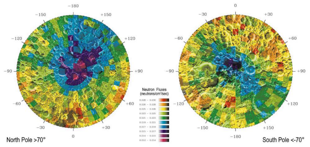
Figure 2.
HardPix with TimePix3 sensor visible in the entrance window.
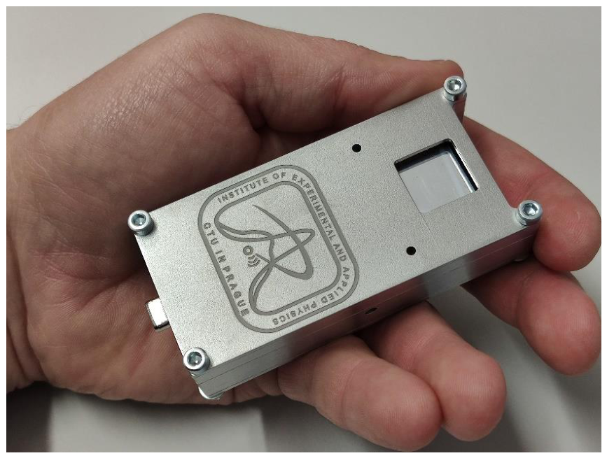
Figure 3.
Neutron flux on the lunar surface for different water mass fractions calculated with Geant4/PLANETOCOSMICS for primary GCR nuclei (Z=1-28) for a) solar minimum conditions, i.e. GCR intensity maximum, and b) solar maximum conditions, i.e. GCR intensity minimum. Figures c) and d) contain the identical neutron flux as a) and b) respectively but in lethargy representation.
Figure 3.
Neutron flux on the lunar surface for different water mass fractions calculated with Geant4/PLANETOCOSMICS for primary GCR nuclei (Z=1-28) for a) solar minimum conditions, i.e. GCR intensity maximum, and b) solar maximum conditions, i.e. GCR intensity minimum. Figures c) and d) contain the identical neutron flux as a) and b) respectively but in lethargy representation.
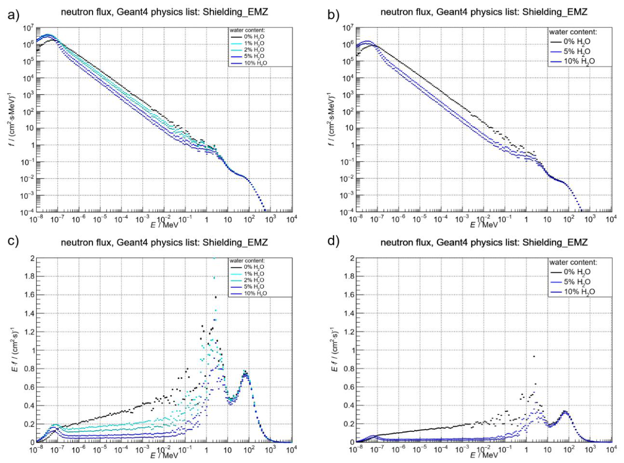
Figure 4.
Thermal (left) and epi-thermal (right) neutron fluence rates calculated for average mare regolith and FAN regolith in dependence on the water content of the regolith. In the layered setup, the wet regolith is covered with a 50 g/cm2 layer of dry regolith.
Figure 4.
Thermal (left) and epi-thermal (right) neutron fluence rates calculated for average mare regolith and FAN regolith in dependence on the water content of the regolith. In the layered setup, the wet regolith is covered with a 50 g/cm2 layer of dry regolith.
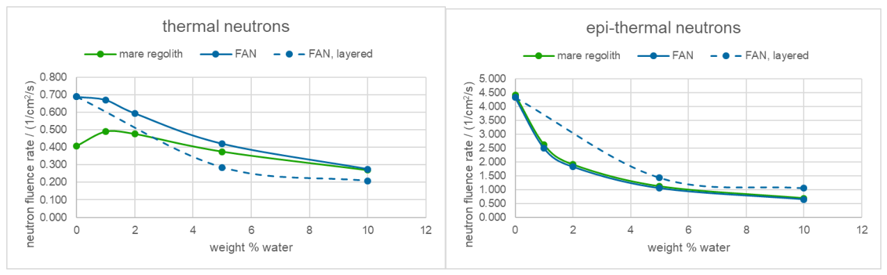
Figure 5.
Thermal and fast neutron detection efficiencies of LiF and PE converter layers used with the Timepix3 detector (from [42]).
Figure 5.
Thermal and fast neutron detection efficiencies of LiF and PE converter layers used with the Timepix3 detector (from [42]).
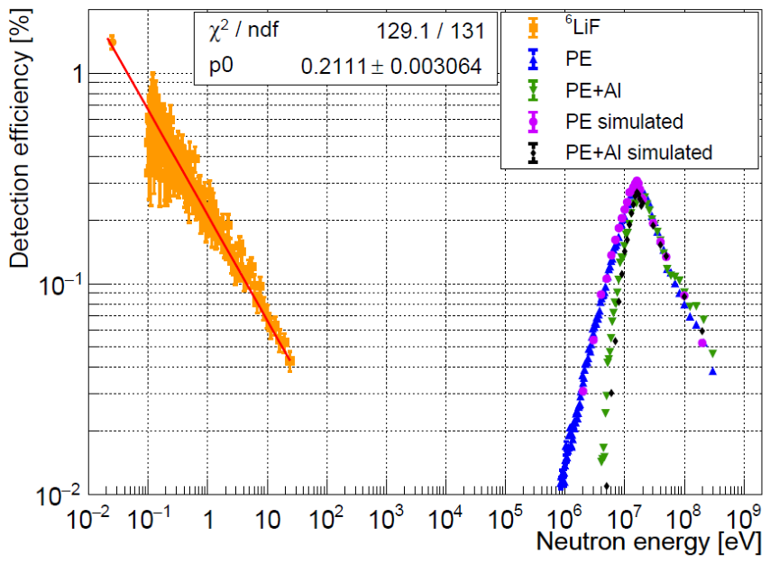
Figure 7.
Pictures of the experimental setup in the AmBe measurement. (Left) Timepix3 detector located under a layer of white polyethylene bricks that moderate the neutrons from the AmBe source. The AmBe source itself is not visible. (Right) A thin 100 μm thick aluminium foil placed on top of the Timepix3 sensor. Bottom side of the aluminium foil carries the LiF converter layer.
Figure 7.
Pictures of the experimental setup in the AmBe measurement. (Left) Timepix3 detector located under a layer of white polyethylene bricks that moderate the neutrons from the AmBe source. The AmBe source itself is not visible. (Right) A thin 100 μm thick aluminium foil placed on top of the Timepix3 sensor. Bottom side of the aluminium foil carries the LiF converter layer.
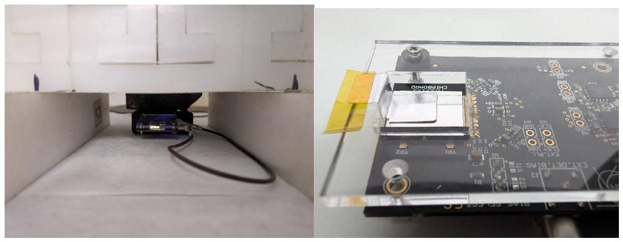
Figure 8.
Clusters of shape "heavy blob" in the 256 × 256 pixel matrix of Timepix3. Color scale shows energy in keV deposited in pixels. The top right region inside the red rectangle shows higher density of heavy blobs – it is where the LiF converter was located, and most of these heavy blobs were created by tritium and helium nuclei from the conversion. Heavy blobs in the region without LiF converter come from the background (e.g. alpha particles from radon gas).
Figure 8.
Clusters of shape "heavy blob" in the 256 × 256 pixel matrix of Timepix3. Color scale shows energy in keV deposited in pixels. The top right region inside the red rectangle shows higher density of heavy blobs – it is where the LiF converter was located, and most of these heavy blobs were created by tritium and helium nuclei from the conversion. Heavy blobs in the region without LiF converter come from the background (e.g. alpha particles from radon gas).
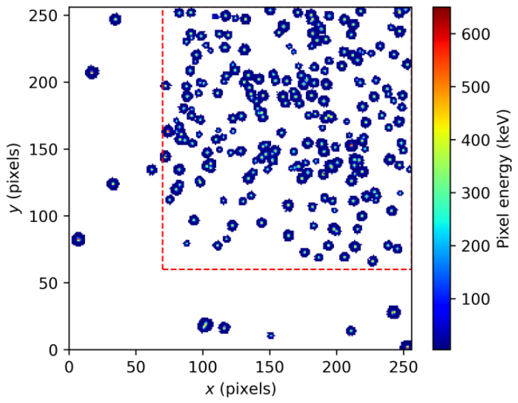
Figure 9.
Energy spectrum of heavy blobs under LiF region (red) compared to the energy spectrum of heavy blobs in the control region (blue). The blue spectrum was scaled by a constant to match the red spectrum at high energies.
Figure 9.
Energy spectrum of heavy blobs under LiF region (red) compared to the energy spectrum of heavy blobs in the control region (blue). The blue spectrum was scaled by a constant to match the red spectrum at high energies.
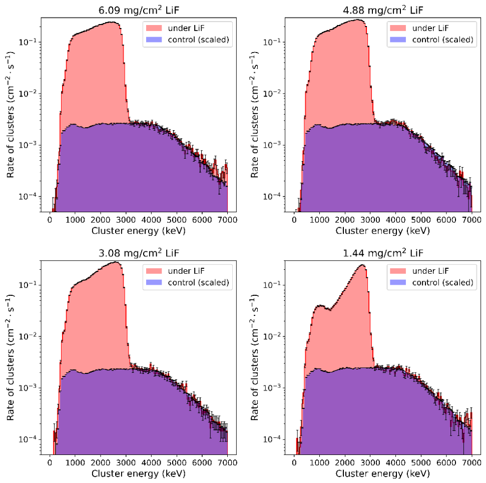
Figure 10.
Comparison of the rate of tritium and helium products of 6Li + n interactions under LiF layers of different thicknesses. Red data points show results from measurements taken at the beginning of October 2024. The blue data points are from the end of October 2024, when we repeated a few measurements to prove that we can consistently reproduce the same conditions. Errors were estimated by dividing the sensor area under the LiF converter into 9 distinct areas of roughly the same size, calculating the rate of tritium and helium heavy blobs in each of them, and calculating the standard deviation of these nine rates. The 4.88 mg cm−2 LiF layer gives the highest rate of tritium and helium nuclei (8.85 ± 0.27) cm−2 s−1, given by the weighted average of the two measurements.
Figure 10.
Comparison of the rate of tritium and helium products of 6Li + n interactions under LiF layers of different thicknesses. Red data points show results from measurements taken at the beginning of October 2024. The blue data points are from the end of October 2024, when we repeated a few measurements to prove that we can consistently reproduce the same conditions. Errors were estimated by dividing the sensor area under the LiF converter into 9 distinct areas of roughly the same size, calculating the rate of tritium and helium heavy blobs in each of them, and calculating the standard deviation of these nine rates. The 4.88 mg cm−2 LiF layer gives the highest rate of tritium and helium nuclei (8.85 ± 0.27) cm−2 s−1, given by the weighted average of the two measurements.
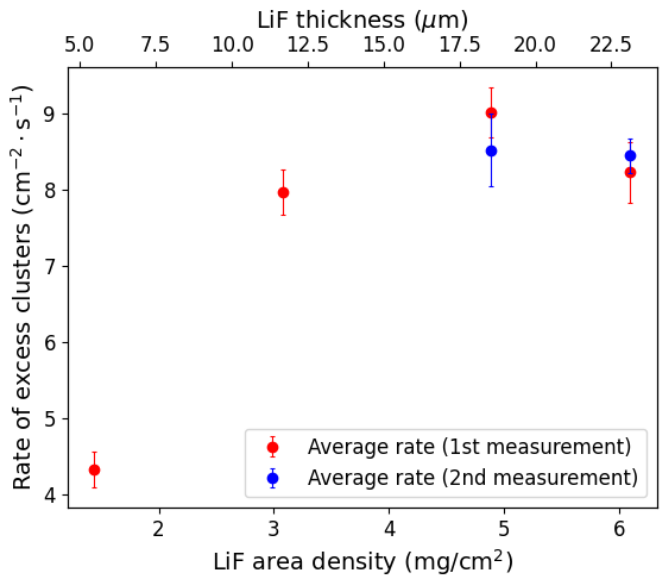
Figure 11.
Timepix3 detector with 1 mm thick cadmium metal shielding wrapped around the sensor. There were openings on sides of the sensor, but the sleeve had ∼1 cm excess on both sides of the openings.
Figure 11.
Timepix3 detector with 1 mm thick cadmium metal shielding wrapped around the sensor. There were openings on sides of the sensor, but the sleeve had ∼1 cm excess on both sides of the openings.
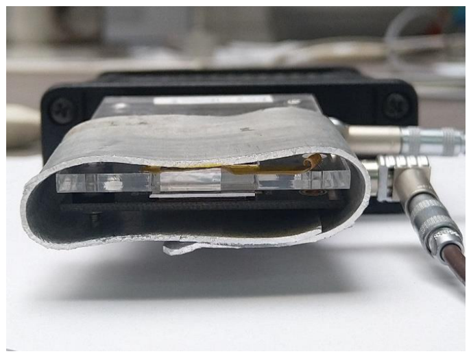
Figure 12.
A graphite pile at CMI with 6 AmBe sources inserted around the detector in the middle.
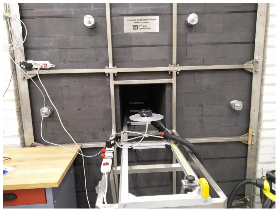
Figure 13.
The plot of the average rate of heavy clusters under the LiF converter as a function of the converter thickness measured at CMI. Left vertical axis shows the absolute flux of heavy blobs while the right axis shows the flux as a percentage of the total neutron fluence rate (1.448 ± 0.018) × 104 cm−2 s−1. The blue points measurements with cadmium shielding were likely contaminated by some thermal neutrons that passed through the openings in the shielding. The blue points are thus only upper estimates. The error bars were calculated in the same way as in Figure 10.
Figure 13.
The plot of the average rate of heavy clusters under the LiF converter as a function of the converter thickness measured at CMI. Left vertical axis shows the absolute flux of heavy blobs while the right axis shows the flux as a percentage of the total neutron fluence rate (1.448 ± 0.018) × 104 cm−2 s−1. The blue points measurements with cadmium shielding were likely contaminated by some thermal neutrons that passed through the openings in the shielding. The blue points are thus only upper estimates. The error bars were calculated in the same way as in Figure 10.
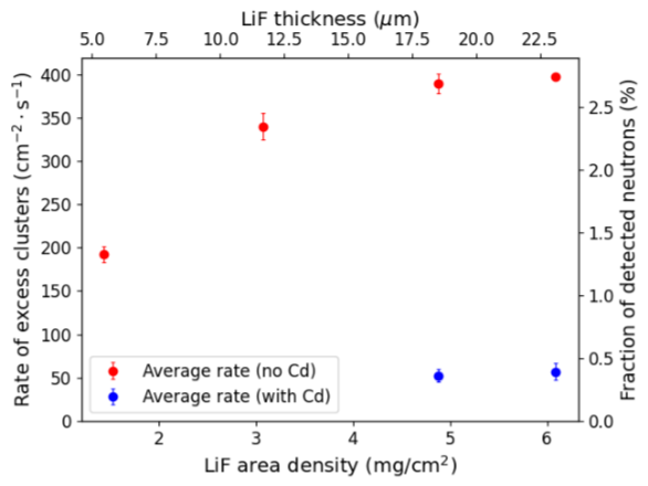
Figure 14.
Density of heavy blobs in the measurement at CMI with the cadmium shielding. The LiF converter was placed in the upper right corner of the sensor. The density of heavy blobs under LiF is ∼1.5 higher in the upmost region compared to the lowest region.
Figure 14.
Density of heavy blobs in the measurement at CMI with the cadmium shielding. The LiF converter was placed in the upper right corner of the sensor. The density of heavy blobs under LiF is ∼1.5 higher in the upmost region compared to the lowest region.
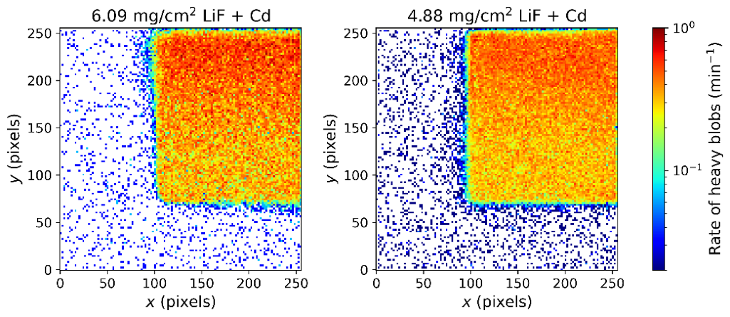
Figure 15.
Lethargy fluxes of neutrons based on physic list and water composition extracted from Figure 3.
Figure 15.
Lethargy fluxes of neutrons based on physic list and water composition extracted from Figure 3.
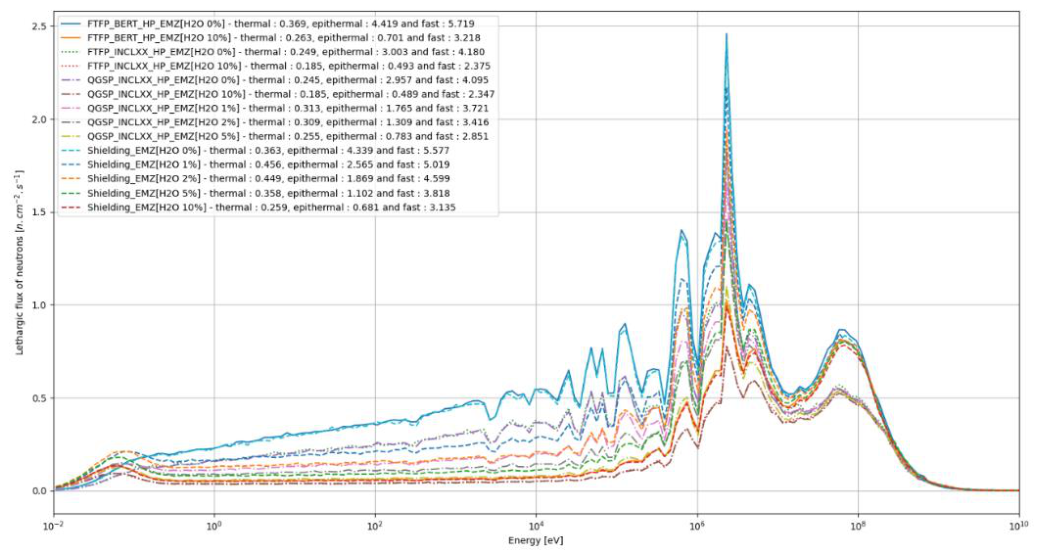
Figure 16.
Comparison of the total fluence rate of neutrons (upper left), fluence rate of thermal neutrons (upper right), epithermal neutrons (lower left) and fast neutrons (lower right) according to the water content and the physics list used.
Figure 16.
Comparison of the total fluence rate of neutrons (upper left), fluence rate of thermal neutrons (upper right), epithermal neutrons (lower left) and fast neutrons (lower right) according to the water content and the physics list used.
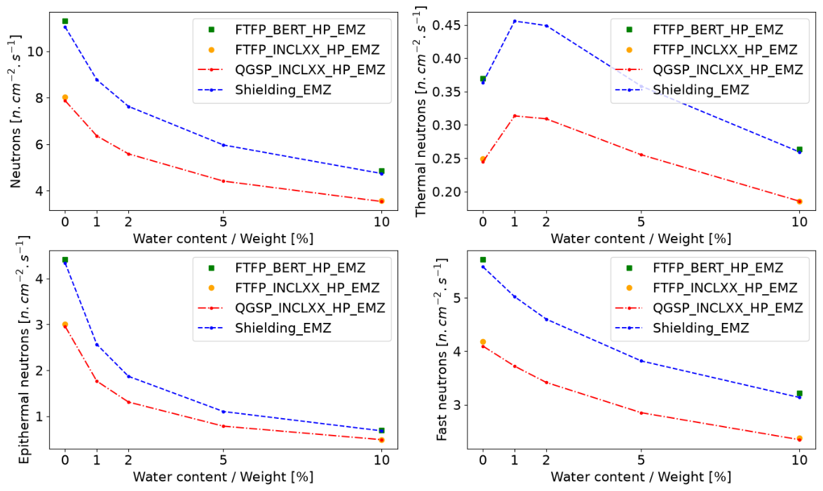
Figure 17.
Neutrons detection efficiencies measured (full lines) versus simulated conversion layers (markers) in percentage of water mass ratio in regolith according to the neutron energy: blue for thermal, red for epithermal and green for fast neutrons. The small shift in fast neutron simulation vs measurement might be explained by the fact that simulations used 2 mm of PE converter while the measurements were done using 1 mm of PE.
Figure 17.
Neutrons detection efficiencies measured (full lines) versus simulated conversion layers (markers) in percentage of water mass ratio in regolith according to the neutron energy: blue for thermal, red for epithermal and green for fast neutrons. The small shift in fast neutron simulation vs measurement might be explained by the fact that simulations used 2 mm of PE converter while the measurements were done using 1 mm of PE.
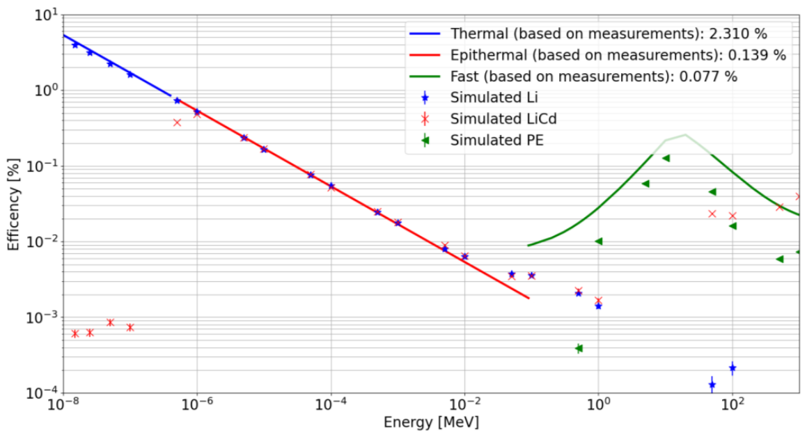
Figure 18.
Estimated count rates detected by the Neutron HardPix based on the water content and the measured efficiency.
Figure 18.
Estimated count rates detected by the Neutron HardPix based on the water content and the measured efficiency.
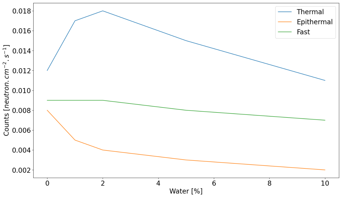
Figure 19.
Water content predictions at 3σ precisions according to the number of detected neutrons over measurement time.
Figure 19.
Water content predictions at 3σ precisions according to the number of detected neutrons over measurement time.
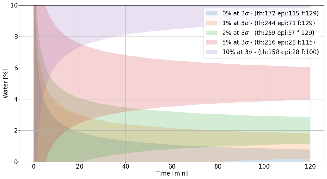
Figure 20.
1 MeV neutron beam moderated by 30 cm of SiO2 and 1 cm thick sheets of PE. Detectors with Timepix3 sensor are visible on the left.
Figure 20.
1 MeV neutron beam moderated by 30 cm of SiO2 and 1 cm thick sheets of PE. Detectors with Timepix3 sensor are visible on the left.
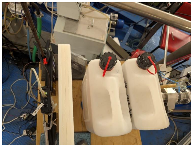
Figure 22.
Measured count rates of epithermal (left) and thermal+epithermal (right) neutrons showed as blue dots vs simulated count rates for each setup - 30 cm SiO2 + 1.8, 2.8, 3.8 and 4.8 cm PE represented by the regolith with 1, 2, 5 and 10 % of water content.
Figure 22.
Measured count rates of epithermal (left) and thermal+epithermal (right) neutrons showed as blue dots vs simulated count rates for each setup - 30 cm SiO2 + 1.8, 2.8, 3.8 and 4.8 cm PE represented by the regolith with 1, 2, 5 and 10 % of water content.
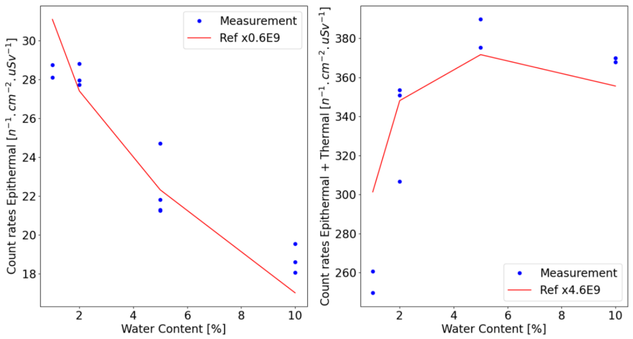
Table 1.
Elemental mass fractions used in the model calculations for the different water content. The first line represents the regolith without water and was calculated from Table 6.3 (Mare) in [36].
| Elemental mass fraction in regolith | |||||||||
| H2O mass fraction | H | O | Na | Mg | Al | Si | Ca | Ti | Fe |
| 0.00 | 0.0000 | 0.4317 | 0.0041 | 0.0555 | 0.0785 | 0.2124 | 0.0843 | 0.0236 | 0.1100 |
| 0.01 | 0.0011 | 0.4363 | 0.0041 | 0.0549 | 0.0777 | 0.2103 | 0.0834 | 0.0233 | 0.1089 |
| 0.02 | 0.0022 | 0.4408 | 0.0040 | 0.0544 | 0.0769 | 0.2082 | 0.0826 | 0.0231 | 0.1078 |
| 0.05 | 0.0056 | 0.4545 | 0.0039 | 0.0527 | 0.0745 | 0.2018 | 0.0801 | 0.0224 | 0.1045 |
| 0.10 | 0.0112 | 0.4773 | 0.0037 | 0.0499 | 0.0706 | 0.1912 | 0.0759 | 0.0212 | 0.0990 |
Table 2.
Neutron fluence rates on the lunar surface from primary GCR calculated for solar minimum conditions and different water content in the regolith and Geant4 physics list Shielding_EMZ.
Table 2.
Neutron fluence rates on the lunar surface from primary GCR calculated for solar minimum conditions and different water content in the regolith and Geant4 physics list Shielding_EMZ.
| Solar minimum | ||||||
| E < 0.48 eV | 0.48 eV ≤ E < 0.1 MeV | total | ||||
| H2O mass fraction | f / (cm2∙s)-1 | Δ wrt. 0% H2O / % | f / (cm2∙s)-1 | Δ wrt. 0% H2O / % | f / (cm2∙s)-1 | Δ wrt. 0% H2O / % |
| 0.00 | 0.409 | 0.0 | 4.410 | 0.0 | 10.977 | 0.0 |
| 0.01 | 0.490 | 19.9 | 2.615 | -40.7 | 8.719 | -20.6 |
| 0.02 | 0.476 | 16.5 | 1.907 | -56.8 | 7.582 | -30.9 |
| 0.05 | 0.376 | -8.0 | 1.125 | -74.5 | 5.931 | -46.0 |
| 0.10 | 0.270 | -33.9 | 0.697 | -84.2 | 4.709 | -57.1 |
Table 3.
Neutron fluence rates on the lunar surface from primary GCR calculated for solar maximum conditions and different water content in the regolith and Geant4 physics list Shielding_EMZ.
Table 3.
Neutron fluence rates on the lunar surface from primary GCR calculated for solar maximum conditions and different water content in the regolith and Geant4 physics list Shielding_EMZ.
| Solar maximum | ||||||
| E < 0.48 eV | 0.48 eV ≤ E < 0.1 MeV | total | ||||
| H2O mass fraction | f / (cm2∙s)-1 | Δ wrt. 0% H2O / % | f / (cm2∙s)-1 | Δ wrt. 0% H2O / % | f / (cm2∙s)-1 | Δ wrt. 0% H2O / % |
| 0.00 | 0.197 | 0.0 | 2.022 | 0.0 | 4.782 | 0.0 |
| 0.05 | 0.164 | -16.9 | 0.472 | -76.7 | 2.459 | -48.6 |
| 0.10 | 0.112 | -43.2 | 0.280 | -86.1 | 1.912 | -60.0 |
Table 7.
Neutron fluence rates on the lunar surface from primary GCR calculated for solar minimum conditions and different water content in the FAN regolith and the layered geometry.
Table 7.
Neutron fluence rates on the lunar surface from primary GCR calculated for solar minimum conditions and different water content in the FAN regolith and the layered geometry.
| Solar minimum | ||||||
| E < 0.48 eV | 0.48 eV ≤ E < 0.1 MeV | total | ||||
| f / (cm2∙s)-1 | uncertainty | f / (cm2∙s)-1 | uncertainty | f / (cm2∙s)-1 | uncertainty | |
| H2O mass fraction | FAN regolith: Geant4 physics list:Shielding_EMZ | |||||
| 0.00 | 0.6902 | 0.0032 | 4.3183 | 0.0082 | 10.6359 | 0.0138 |
| 0.01 | 0.6717 | 0.0028 | 2.4882 | 0.0055 | 8.3086 | 0.0110 |
| 0.02 | 0.5950 | 0.0025 | 1.8234 | 0.0043 | 7.2253 | 0.0095 |
| 0.05 | 0.4207 | 0.0019 | 1.0552 | 0.0030 | 5.6163 | 0.0076 |
| 0.10 | 0.2754 | 0.0014 | 0.6511 | 0.0022 | 4.4625 | 0.0065 |
| Layered FAN regolith: Geant4 physics list:Shielding_EMZ | ||||||
| H2O mass fraction | f / (cm2∙s)-1 | uncertainty | f / (cm2∙s)-1 | uncertainty | f / (cm2∙s)-1 | uncertainty |
| 0.05 | 0.2854 | 0.0016 | 1.4364 | 0.0037 | 6.4639 | 0.0085 |
| 0.10 | 0.2078 | 0.0013 | 1.0633 | 0.0029 | 5.8167 | 0.0075 |
Disclaimer/Publisher’s Note: The statements, opinions and data contained in all publications are solely those of the individual author(s) and contributor(s) and not of MDPI and/or the editor(s). MDPI and/or the editor(s) disclaim responsibility for any injury to people or property resulting from any ideas, methods, instructions or products referred to in the content. |
© 2026 by the authors. Licensee MDPI, Basel, Switzerland. This article is an open access article distributed under the terms and conditions of the Creative Commons Attribution (CC BY) license (http://creativecommons.org/licenses/by/4.0/).
Copyright: This open access article is published under a Creative Commons CC BY 4.0 license, which permit the free download, distribution, and reuse, provided that the author and preprint are cited in any reuse.