

Submitted:
14 July 2026
Posted:
15 July 2026
You are already at the latest version
Abstract
Simple memristive circuits are attractive chaos sources for secure communication, random-number generation, and chaotic sensing. Reliable operation, however, requires knowing where in parameter space the chaos persists and where periodic windows or coexisting attractors make it fragile. This paper constructs an operating map for an improved memristive diode-bridge band-pass-filter circuit in its two accessible tuning parameters, set by the filter capacitance and the feedback resistance ratio. Two-parameter bifurcation maps and Lyapunov exponent fields give the global layout of the plane; numerical continuation traces the stable and unstable periodic-orbit branches that organise it; and phase portraits, power spectra, component-level SPICE simulation, and prototype measurements characterise representative regimes. The plane separates into broad chaotic regions, higher-period windows, a period-adding window, and a multistability zone. A chaotic interval is reported as robust chaos only when the tracked periodic branches are all unstable, the Lyapunov exponent is positive throughout, and initial-condition scans detect no coexisting attractor; the continuation shows the same period-doubling mechanism bounding the chaotic regions in both parameters. Mapping the dimensionless results to component values yields design guidance for reaching candidate robust-chaos regions and avoiding fragile and multistable zones, including a hardware-confirmed limit on inductor loss beyond which the chaotic band collapses.
Keywords:
memristive circuit
; diode bridge
; bifurcation analysis
; numerical continuation
; period-doubling locus
; Lyapunov exponent
; period-adding
; robust chaos
; multistability
; Poincaré map
1. Introduction
Chaotic signals generated by simple analogue electronic circuits remain attractive for secure communication, entropy and random-number generation, chaotic sensing, and related low-complexity signal-generation tasks [1,2]. For these applications, chaos at an isolated parameter value is not sufficient: the chaotic regime should persist over a useful component range and tolerate drift, manufacturing spread, and noise. Periodic windows and coexisting attractors make a nominally chaotic source unreliable, because a small parameter change or a different initial condition can switch the observed response to another mode. The property a designer needs is therefore robust chaos — chaos that persists over an open parameter range without embedded periodic windows or coexisting attractors [3], the operating counterpart of the unstable-periodic-orbit description used in complete-bifurcation-group analyses of related oscillators [1]. We make this notion precise in Section 2.3 and use it as the criterion for separating dependable from fragile operating regions.
Memristive and memristor-inspired circuits are a particularly rich source of such dynamics, because the memristive element supplies a strong nonlinear memory effect in compact form [4,5,6]. The improved memristive diode-bridge band-pass-filter circuit is a representative third-order example and a useful benchmark topology: it has a simple component-level realisation, an established mathematical model, a known nominal route containing period-1 (P1), period-2 (P2), chaotic, and period-3 (P3) behaviour, and reported coexisting attractors [7]. Related band-pass, Chua, jerk, hyperjerk, and filter topologies based on diode-bridge memristive elements have likewise shown period-doubling cascades, Lyapunov-positive chaos, bursting, coexisting bifurcation modes, basins of attraction, and circuit-level or hardware-oriented multistability [5,6,8,9,10,11,12,13,14,15,16]. These studies make clear that neither chaos nor multistability alone is new in this circuit family.
What is missing is an operating map that tells a designer where chaotic behaviour is likely to persist and where periodic or multistable windows make operation fragile. Existing two-parameter diode-bridge results demonstrate the value of sampled periodicity maps, but sampled maps alone do not identify the stable and unstable periodic branches that organise the observed structure.
The main contribution is a continuation-supported operating map for the memristive diode-bridge band-pass-filter circuit. The paper combines sampled bifurcation maps, Lyapunov estimates, periodic-orbit continuation, and representative time-domain and spectral views to distinguish broad chaotic regions from narrow periodic and multistable ones. The parameter-to-component mapping, a component-level SPICE check, and hardware measurements on a prototype board then connect the numerical structure to practical circuit choices.
The rest of the paper is organised as follows. Section 2 describes the circuit, dimensionless model, equilibrium properties, and numerical workflow. Section 3 presents the results in the following order: maps, continuation-supported branch structure, cross-sections, representative regimes, multistability, SPICE simulation, and hardware measurements. Section 4 discusses practical operating guidance and limitations, and Section 5 summarises the conclusions.
2. Materials and Methods
2.1. Circuit Model and Dimensionless Parameters
The circuit is a second-order active band-pass filter in which one series resistor is replaced by an improved memristive diode-bridge emulator — a diode bridge cascaded with a single inductor — which supplies the system's nonlinearity [7]. Figure 1 shows the schematic: the operational-amplifier band-pass stage, the feedback resistors Ri and Rf that set the filter gain, the matched filter capacitors C1 = C2 = C, and the diode-bridge emulator connected between port +1 and the op-amp inverting port -1'. The two capacitor voltages and the emulator inductor current form a third-order autonomous system.
With the dimensionless state (x, y, z) proportional to the two capacitor voltages and the emulator inductor current, the governing equations are
with dimensionless parameters
where a is the primary bifurcation parameter, c sets the diode-bridge scale, and k is the band-pass feedback ratio. Here C denotes the matched filter capacitance varied as C1 = C2 = C, as in the original circuit sweep [7]. The remaining symbols are physical quantities of the emulator carried over from the original model [7]: R is the band-pass series resistance that the diode-bridge emulator replaces, IS is the reverse saturation current of the four bridge diodes, and ρ = 1 / (2 n VT) is fixed by their emission coefficient n and thermal voltage VT. The 1N4148 diode values used by Xu et al. are IS = 5.84 nA, n = 1.94, and VT = 25 mV, giving ρ ≈ 10.31 V-1; with R = 50 Ω this reproduces the nominal c = 2 ρ R IS ≈ 6.02 × 10⁻⁶. Throughout this work c was held fixed at this nominal value, and the analysis focused on the (a, k) plane. For hardware interpretation with R = 50 Ω and L = 10 mH, the capacitance-controlled parameter maps to component values as
so that the dimensionless windows identified numerically correspond to concrete matched-capacitor selections. For other inductor values the mapping follows from a = R2 C/L.
The model is invariant under the reflection (x, y, z) → (-x, -y, z): the hyperbolic terms satisfy tanh(-(y-x)) = -tanh(y-x) and cosh(-(y-x)) = cosh(y-x), so the two in-plane equations change sign together while the z equation is unchanged. Coexisting attractors are therefore either self-symmetric or occur as mirror pairs, a fact used in the interpretation of multistability below.
2.2. Equilibrium and Local Stability
Setting the right-hand sides to zero shows that the origin O = (0, 0, 0) is the only equilibrium: since c + z > 0, the first equation forces y = x, the third then forces z = 0, and the second finally forces x = 0. Linearising about the origin gives the block-diagonal Jacobian
The inductor-current direction z decouples with the real eigenvalue -a/c, while the in-plane block has trace k - 2c and determinant c, so that
For the parameter ranges studied here (c = 6.02 × 10⁻⁶, k ∈ [0.02, 0.08], a ∈ [0.001, 0.08]), the decoupled eigenvalue -a/c is large and negative — of order -102 to -104, the origin of the system's numerical stiffness — while λ1,2 are real and positive. The origin is therefore an index-2 saddle with a two-dimensional unstable manifold and a one-dimensional, very fast stable manifold; no stable equilibrium exists. The attractors reported below are reached from initial conditions near this saddle's unstable manifold and are in that sense self-excited rather than hidden, in the terminology of Leonov and Kuznetsov [17]. The absence of a stable equilibrium does not by itself rule out hidden attractors elsewhere in the state space.
2.3. Numerical Analysis Workflow
The Poincaré section was the hyperplane y = 0, sampled on upward crossings and projected to the (x, z) plane. The resulting return map is the object used by both the brute-force and continuation stages. Global maps were computed first, continuation was then applied to the organising periodic branches, and local simulations illustrated selected regimes. A subset of the identified regimes was additionally checked with component-level SPICE simulation of the diode-bridge/op-amp circuit (Section 3.12) and with measurements on a prototype board (Section 3.13).
Two-parameter bifurcation maps were computed in the (a, k) plane by detecting the periodicity of the Poincaré return points on dense parameter grids. Each grid point was integrated from two fixed initial conditions placed symmetrically about the origin: a positive seed (x0, y0, z0) = (0, +0.01, 0) and a negative seed (0, -0.01, 0). Because of the reflection symmetry (Section 2.1), the two seeds can reach different coexisting attractors; retaining both exposes the symmetry-organised multistability and guards against seed-dependent artefacts in the periodicity patterns. The largest Lyapunov exponent of the Poincaré return map was estimated by the two-trajectory method with periodic renormalisation [18], both as a field over the (a, k) plane and as a one-parameter diagram along the nominal slice k = 0.05. The two-seed maps serve as the survey layer of the analysis; statements about coexistence rest on the continued branches, on a recomputation of the map from a wider seed set, and on initial-condition censuses at selected operating points (Section 3.1).
Stable and unstable periodic branches were obtained by pseudo-arclength continuation of the Poincaré return map [19,20], combined with an automated reconnaissance-and-seeding stage that discovers candidate branches and a targeted refinement stage applied to the organising families. Continuation follows each branch through fold and period-doubling bifurcations and along its unstable segments, recovering the unstable orbits and narrow stable windows that brute-force sampling misses, so that the orbits organising each region can be overlaid on the sampled clouds. Floquet multipliers of the return map were tracked to locate period-doubling bifurcations, whose loci were continued across k where branch coverage was reliable. Dense one-parameter brute-force cross-sections provided the background clouds for the continuation-supported diagrams. Branch overlays were accepted only when consistent with the brute-force cloud and, for narrow structures such as the nominal mixed region, with direct period validation at representative parameter values. Finally, power spectra, time series, and phase portraits of representative regimes were computed from uniformly sampled trajectories.
We use robust chaos in an operational sense, not as a synonym for a single positive Lyapunov estimate. Following the robust-chaos concept of Banerjee, Yorke, and Grebogi [3] and the complete-bifurcation-group description applied to related oscillators [1], a chaotic parameter interval is called robust when it forms an unstable periodic infinitium (UPI): an interval bounded by a period-doubling cascade whose periodic skeleton — the set of periodic orbits embedded in the attractor — contains only unstable orbits, so that the chaotic motion is not interrupted by stable periodic windows; the label UPI-n identifies the period-n cascade from which the interval grows. In practice an interval is reported as robust chaos only when three conditions, all readable from the cross-sections and the representative attractors, hold together: (i) the largest Lyapunov exponent is positive throughout the interval; (ii) the continued periodic branches over the interval carry no stable segment, so there is no embedded periodic window; and (iii) the regime is a single attractor with no coexisting partner, ideally a wide one-piece (single-band) attractor. Conditions (i) and (ii) are read from the Lyapunov diagrams and the continued branches; condition (iii) is tested with the wider-seed map probe and the initial-condition censuses of Section 3.1. Where the coexistence test rests on the sampled maps alone, the interval is reported as a candidate robust-chaos region. Intervals that are chaotic by the Lyapunov criterion alone but contain embedded periodic windows, coexisting attractors, or narrow higher-period islands are reported as fragile or mixed regions, not as robust chaos.
2.4. Implementation and Reproducibility
All computations were carried out in Julia (https://julialang.org/). The stiff behaviour near the origin saddle was handled with a stiffness-aware adaptive solver — the auto-switching AutoTsit5(Rosenbrock23()) integrator — and a floor of 10-12 on c + z guarded the logarithm against transient integrator overshoot. Across the representative regimes of Section 3 the integrated trajectories keep c + z above 4 × 10⁻⁶ and never engage the guard, and repeating the computations with the floor moved between 10-15 and 10-8, or removed entirely, leaves the detected periods and Lyapunov exponents unchanged. Parameter sweeps and map computations were parallelised across cores. Unless otherwise stated, integrations used tolerances reltol = abstol = 10-8. Each figure is tied to a recorded parameter configuration; the principal numerical settings are collected in Table 1, and the software versions used are listed beneath it.
Software: Julia 1.12.6; DynamicsKit.jl 0.1.2 (analysis library; openly archived at https://doi.org/10.5281/zenodo.21327846); BifurcationKit.jl 0.7.3 (continuation); OrdinaryDiffEq.jl 7.1.0 / DifferentialEquations.jl 8.0.1 (integration); ForwardDiff.jl 1.4.1 (Jacobians); JLD2.jl 0.6.4 (artefact storage); Plots.jl 1.41.6 with the GR 0.73.26 backend (figures).
3. Results
3.1. Global Organisation and Behaviour Regions of the (a, k) Plane
Figure 2 gives the global two-parameter overview, pairing the bifurcation maps (top row) with the corresponding largest Lyapunov exponent fields (bottom row) for both seeds. Comparable maps and Lyapunov fields exist for related diode-bridge circuits [8,12]; here, these maps serve as the substrate for the continuation-traced branch structure of Section 3.2. The period counts and spatial patterns agree closely between the positive and negative seeds.
Four kinds of regions organise the plane. First, a low-period backbone: period-1 motion (orange) fills a large region at high capacitance, with the high-a P1 boundary moving from a ≈ 0.045 at k = 0.02 to a ≈ 0.067 at k = 0.05 and a ≈ 0.079 near k = 0.07; at the top of the plotted k range the high-a edge has already entered the period-2 stripe rather than remaining P1. Further low-period zones also occur at small a. These low-period regions coincide with the negative-exponent (blue) parts of the Lyapunov field. Second, a broad chaotic belt runs diagonally across the centre of the plane, 0.02 ≲ a ≲ 0.05 and widening as k increases; it carries the strongest positive exponents (largest exponent reaching 0.75-1.0, deep red) and is the principal robust-chaos candidate. Third, the boundary between them is a period-doubling cascade: the high-a period-1 region is separated from the chaotic belt by a narrow period-2 stripe (green) edged by a thin period-4 sliver (magenta), so that crossing from high toward lower a follows a P1 → P2 → P4 → chaos sequence, and this boundary coincides with the zero-exponent contour of the Lyapunov field. Fourth, periodic windows interrupt the chaotic belt — most visibly the brown period-3 tongues near a ≈ 0.025-0.05 — while a qualitatively distinct period-adding corner of coherent period-5 with period-3, -7, and -9 substructure occupies the low-a, high-k corner (a ≈ 0.005-0.013, k ≳ 0.055).
The dependence of this organisation on the mapping seeds was checked by recomputing the map at reduced resolution (101 × 101) from eight additional initial conditions spread across the attractor region, with the classification settings of Table 1. Every seed reproduces the class shares and region boundaries of Figure 2; about 5% of individual cells change class between seeds, falling to 2% when boundary-adjacent cells are excluded, and re-detection with extended transients confines the persistent differences to structures treated below: the multistability zone of Section 3.10, the period-adding corner, and the borders of the period-3 tongues. The tongue borders carry genuine coexistence — at a ≈ 0.024, k ≈ 0.030-0.033 three of the additional seeds converge to a stable period-3 orbit that persists through 104-return transients while the mapping seeds follow chaotic motion — so the tongue basins extend beyond the tongues' footprint in the two-seed map. Initial-condition censuses at four anchors of the central belt (k = 0.05, a = 0.034-0.052, 41 × 41 grids in (x0, z0) at both signs of y0) complete the check. At a = 0.034, 0.040, and 0.046 every census cell that initially reports a periodic class unlocks to the chaotic attractor under extended transients (all within 104 returns); the period-4 patches at a = 0.046 are trajectories locking temporarily near the unstable period-4 branch recovered by the continuation of Section 3.3 before joining the chaotic attractor, with the longest locking episodes exceeding 3000 returns. At a = 0.052, next to the period-3 window edge, the flagged cells concentrate in the period-3 family (about 9% of initial conditions at the census budget); under extended transients most of these read chaotic, and the few that still read period-3, -6, or -9 at 104 returns shift their detected period between budgets — intermittent locking episodes near the adjacent window, which already shapes the dynamics at this anchor.
A substantial part of the studied region has a positive Lyapunov exponent. The robust-chaos candidates in the sense of Section 2.3 are the interior of the central belt — the deep-red zone away from the embedded period-3 tongues and from the period-doubling boundary — whereas the narrow periodic stripes, the embedded tongues, and the period-adding corner are the fragile regions to be avoided for a chaos source. The following sections take these regions in turn, using a one-parameter cross-section through each as evidence for the branch structure that produces it.
3.2. Branch Structure Underlying the Map
Figure 3 overlays the two principal period-doubling loci — P1 → P2 and P2 → P4 — on the Lyapunov field. Each locus is traced across k by finding where a Floquet multiplier of the return map crosses the unit circle. The two loci follow the lower-a boundary of the broad chaotic band and move toward larger a as the feedback ratio is increased. This lower-a doubling boundary is separate from the high-a P1 edge described from the global map in Section 3.1. The loci show that the entry into chaos across most of the plane is organised by a period-doubling cascade; they are traced over the range where they remain single-valued.
In the one-parameter continuation-supported diagrams below, pale-cyan dots show the brute-force cross-section, stable periodic branches are blue, and unstable branches are red. A bifurcation group nT denotes the set of interconnected stable and unstable regimes originating from period n [1]; the diagrams are continuation-supported, so group and UPI labels mark the recovered branch structure only. Where the same period appears more than once in a figure, the period label carries an instance subscript: in the seed-paired diagrams of Section 3.3 and Section 3.5, and 3.7 the subscript indexes the coexisting family, with P2₁ belonging to the negative-seed family and P2₂ to the positive-seed family, while in the feedback-ratio diagrams of Section 3.4, where both coexisting sheets appear in every panel, it indexes the sheet.
3.3. Cross-Section at k = 0.05 — the Nominal Route
The first cross-section is the nominal slice k = 0.05, along which the published route was originally reported [7]. Figure 4 makes that route quantitative: the upper panels overlay the continued P1, P2, P3, and P4 branches on the one-parameter brute-force diagram in a for both seeds, and the lower panels show the corresponding largest Lyapunov exponent with the representative operating points marked on both diagrams. The continuation shows the stable P1 branch losing stability and the P2 and P4 branches doubling and then continuing as unstable orbits (red) through much of the chaotic band: where the positive-exponent interval contains no recovered stable low-period segment, the tracked periodic skeleton has the branch-level signature of the robust-chaos (UPI) criterion of Section 2.3, and the initial-condition censuses of Section 3.1 support the single-attractor condition at anchors inside this band. The exponent is non-positive in the low-a periodic regime and becomes positive across the broad chaotic band, while higher-period windows appear as sharp returns toward non-positive values. This route reproduces the P1 → P2 → chaos → P3 sequence reported originally [7] and provides the quantitative backbone for the rest of the study.
At very small a, finite-time exponent estimates near the origin saddle are unreliable because of stiffness; this region is periodic and the exponent is not displayed there. The narrow structures away from the broad chaotic band are examined in the focused windows of Section 3.5, Section 3.6, Section 3.7 and Section 3.8. The P3 pieces in Figure 4 are fold-bounded, continuation-supported branch segments; nearby branches outside these segments may remain unrecovered. On the high-a side of the UPI-1 interval the recovered P3 arcs carry no seed-observed stable segment: recomputed multiplier checks and direct integrations over a = 0.045-0.056 classify the responses from both seeds as high-period or chaotic.
3.4. Cross-Sections in k (a = 0.05, 0.06) — the Feedback-Ratio Route
The maps and Lyapunov field show strong k-dependence, so Figure 5 presents the complementary cross-section: continuation-supported bifurcation diagrams in the feedback ratio k at two fixed capacitance-controlled values, a = 0.05 and a = 0.06. As k increases from the low-feedback side, the circuit follows the same qualitative sequence as in the a direction: a stable P1 branch loses stability, a stable P2 branch appears, and a further period doubling leads toward chaotic motion. All three coexisting P1 instances are drawn in every panel of Figure 5 and are distinguished by the instance subscript: the doubling-cascade sheet P1₁ → P2₁ → P4₁, the lower sheet P1₂, P2₂, and a third P1 orbit, P1₃, which lies between the two sheets and is unstable over the entire plotted range. At a = 0.05 and k = 0.025, for example, the negative seed settles on the lower-sheet P1₂ orbit near x = -4.49 and the positive seed on the cascade-sheet P1₁ orbit near x = -4.01, and direct integrations confirm that each continued branch is reached from the matching seed. The intervals marked UPI-1 in Figure 5 are candidate robust-chaos intervals: the longest intervals whose continued branches carry no stable low-period segment — k = 0.0449-0.0770 (negative seed) and k = 0.0449-0.080 (positive seed) at a = 0.05, and k = 0.060-0.0728 (negative seed) and k = 0.0589-0.0698 (positive seed) at a = 0.06. They satisfy the branch condition of Section 2.3, but the coexisting seed sheets mean the single-attractor condition is not established there, and the positive-seed interval at a = 0.05 is truncated by the plotted range. At the larger capacitance value, the cascade is shifted to larger k and additional periodic windows are embedded inside the chaotic region. The band-pass feedback ratio is therefore itself a route-to-chaos parameter and provides a resistor-set design knob complementary to capacitance.
3.5. Cross-Section at k = 0.026 — Low-a P4 Window
The first focused window is the low-a window of Figure 6. Along the selected slice, both seeds show a progression from low-period behaviour into a P4-centred window, followed by narrower higher-period and mixed structures. Continuation recovers several accompanying period families, but the refined P4 branch is the dominant organising family. The P2 families are continued from parent P1 branches whose period-doubling points lie just left of the plotted window, at a = 0.0156 for both seeds; the unstable parent P1 continues through the window between the P2 arms in Figure 6c,d. Direct integrations at a = 0.0175-0.0190 reproduce the displaced clouds at larger a: the negative-seed attractor widens across the window, while the positive-seed attractor remains on the coexisting sheet centred near x = -4.36.
3.6. Cross-Section at k = 0.05 — Nominal Mixed P3/P6 Region
Figure 7 shows the nominal mixed window. This region is centred on the transition from the broad P3 response of the nominal route into much narrower higher-period pockets. The branch overlay shows only the portions recovered by continuation and confirmed by direct period detection: a broad P3 window over a = 0.0299-0.03195, a much narrower P6 window immediately beyond it over a = 0.03198-0.03211, and a very local P9 window over a = 0.03243-0.03249, with high-period or chaotic behaviour at a ≥ 0.0325. Disconnected pieces in Figure 7 are locally recovered branches embedded in a mixed region.
3.7. Cross-Section at k = 0.044 — High-a P4 Window
The second higher-period region is shown in Figure 8. The window again contains mixed behaviour and narrow higher-period fragments organised around a P4 family. As in Figure 6, each family's unstable parent P1 branch threads the window between its P2 arms; here the continuation places the parent's return to stability at a = 0.062, just beyond the plotted range, matching the P1 region of the map. This second P4-centred window is separated from the low-a one and not visible from the nominal route alone. At still larger capacitance the dynamics simplify toward low-period oscillation, so these higher-period structures occupy a finite intermediate part of the operating plane.
3.8. Cross-Section at k = 0.078 — P5 Period-Adding Region
A region qualitatively distinct from the period-doubling structure above is found at low capacitance and high feedback ratio. The top row of Figure 9 shows a large coherent P5 region interleaved with P3 and smaller higher-period islands. The continuation-supported slice in the bottom row shows that the P5 response is reached from P3 by a period-adding transition [21] rather than by the period-doubling cascade that organises the main chaotic boundary. This makes the window qualitatively different from the two P4-centred windows. The same region also contains secondary P7 and P9 substructure; P7 is branch-supported in part of the region, while P9 and the narrow P10 island remain local, map-supported features.
3.9. Representative Regimes: Phase Portraits and Spectra
The cross-sections above identify where each regime lives; Figure 10 and Figure 11 show what selected regimes look like in the state plane, time domain, and frequency domain. The chaotic example at a = 0.028 is an anchor point on the published route, not a recommended operating point (Section 4.1).
3.10. Multistability and Coexisting-Attractor Geometry
Symmetry-organised multistability is a hallmark of memristive diode-bridge circuits [9,11,12,22]; Figure 12 shows a representative coexistence of low-period attractors near the nominal route. Consistent with the (x, y, z) → (-x, -y, z) symmetry of Section 2.1, one attractor appears together with its reflection partner while the other is self-symmetric. The basin plot shows that the selected attractor depends on the initial condition in the (x0, z0) section at fixed y0 = 0.01.
3.11. The Published Route as a Single Cross-Section of the Plane
The nominal characterisation of this circuit [7] corresponds to the single slice k = 0.05 of the parameter plane, recovered here in Figure 2 and Figure 4 as a benchmark for the workflow. The two-parameter view shows how much lies beyond that slice: the chaotic band continues across the plane, further higher-period windows lie away from it, and the feedback ratio opens a second route to chaos (Section 3.4).
3.12. Component-Level SPICE Simulation
To check that the numerically identified regimes survive a device-level time-domain solver, the circuit of Figure 1 was implemented directly in ngspice using four 1N4148 diode models, the bridge inductor, matched filter capacitors, and a finite-bandwidth single-pole op-amp macromodel. The macromodel is a differential transconductance stage with open-loop DC gain AOL = 105 and gain-bandwidth product 325 MHz (single pole at GBW/AOL), followed by a soft output-saturation stage Vout = Vrail tanh(v/Vrail) with Vrail = 14 V; input bias current, input offset, and finite input impedance are not modelled. The gain-bandwidth product is set high enough that the macromodel contributes no dynamics of its own in the circuit's kilohertz operating band; re-running the deck with the TL082's 3 MHz value leaves the anchor regimes and the boundaries of the chaotic band unchanged. The diodes use the full SPICE junction model with IS = 5.84 nA, n = 1.94, series resistance 0.568 Ω, junction capacitance Cj0 = 2 pF, and transit time 4 ns, and the bridge inductor carries a 0.1 Ω series resistance. The component deck used the Xu et al. component set [7]: R = 50 Ω, Ri = 50 Ω, Rf = 1 kΩ (k = 0.05), and L = 10 mH. Because diode capacitance, series resistance, and op-amp bandwidth shift the transition points, the capacitance was then swept to locate the same qualitative anchor regimes.
Figure 13 shows the resulting component-level SPICE phase portraits. Period-1, period-2, chaotic, and period-3 responses are recovered at C = 56, 90, 105, and 126 nF, respectively, corresponding to dimensionless values a = R2 C/L of 0.014, 0.0225, 0.02625, and 0.0315. These values track the experimentally reported Xu et al. capacitance sweep (56 nF period-1, 94 nF period-2, 105-115 nF chaos, 126 nF period-3) while allowing for the simplified op-amp macromodel used in ngspice. The result supports the practical circuit interpretation directly: the same regime sequence appears in the realisable diode-bridge/op-amp topology. The netlist and sweep script are provided with the supporting material.
3.13. Hardware Measurements
The circuit of Figure 1 was realised as a prototype board following the component-level deck and Xu et al. [7]: a four-diode 1N4148 bridge feeding the inductor (L = 10 mH; measured winding resistance 27.2 Ω at DC and 29-32 Ω over the operating band, self-resonant frequency 0.7 MHz), R = 50 Ω, Ri = 50 Ω, ±10 V supply rails, a socketed TL082 operational amplifier, and trimmer-set feedback resistance Rf (Figure 14). The capacitor voltages v1 and v2 were recorded differentially with a digital oscilloscope, and the measured waveforms are provided with the supporting material. The mode labels used below were verified against the recorded waveforms with an autocorrelation period test; captures below C = 2 nF, where the oscillation frequency reaches tens of kilohertz and board-level stray capacitance becomes a noticeable fraction of the filter capacitance, are excluded from the model comparison.
Two measured sweeps cover the two routes of the operating map. The capacitance route at Rf = 1 kΩ (k = 0.05) was measured from 0.33 to 690 nF: a structured low-capacitance zone — chaotic responses at 2.2-15 nF, coexisting P2 and P4 attractors at 22 nF, and a P7 window at 26.7 nF — is followed by period-1 (28.8-100 nF), a period-2 window (122-190 nF), and period-1 again up to 690 nF. The feedback-ratio route at fixed C = 100 nF, obtained by reducing Rf from 1 kΩ to 150 Ω (raising k = Ri/Rf), passes through P3 (472 Ω), a period-4 candidate (407 Ω), P2 (346 and 300 Ω), period-11 locking (270 Ω), P3 (250 Ω), chaos (232.3 Ω), P2 (202 Ω), and back to P1 (181 and 150 Ω). Figure 15 shows measured phase portraits of the P1, P2, chaotic, and P3 regimes; their shapes correspond to the component-level SPICE portraits of Figure 13.
The measured capacitance route reproduces the model's entry — the P1 → P2 doubling occurs between C = 100 and 122 nF, above the 88-90 nF anchors of the ideal model and the ideal-inductor SPICE deck — but beyond the period-2 window the board returns to period-1 instead of entering the chaotic band that both predict for C ≈ 96-220 nF. The dominant cause is the inductor's series loss, acting together with the smaller parasitics that every board component contributes. Sweeping the inductor series resistance in the component-level deck collapses the mid-band chaos through a reverse period-doubling: at C = 105 nF chaos persists only below ≈ 10-20 Ω, at C = 160 nF below ≈ 30-45 Ω, and with an effective series resistance of 45 Ω the deck reproduces the measured route almost point-by-point — period-1 at 56-105 nF, a period-2 window at 122-168 nF, and period-1 from 190 nF (the lossy-inductor row of Figure 16a). A Bode 100 impedance sweep of the inductor (100 Hz-1 MHz, impedance adapter; sweep data in the supporting material) measures the loss directly: the series resistance is 27.2 Ω at 100 Hz, matching the DC reading, and rises to 29-32 Ω across the 3-8 kHz operating band, so the inductor alone exceeds the 10-20 Ω collapse threshold. The remaining share of the point-by-point 45 Ω value is a fitted branch-level allowance for losses outside the inductor: wiring and contact resistance, and any amplitude-dependent loss beyond the small-signal sweep. The same argument predicts that chaos survives at low capacitance, where the higher operating frequency raises the inductor's reactance relative to its losses — and the board shows chaos at 2.2-15 nF, together with window structure that the lossy deck reproduces in kind (P2-P4 and P7 windows against the deck's P3, P2, and chaotic pockets at 4.7-33 nF).
Figure 16b applies the same comparison to the feedback-ratio route at C = 100 nF, using brute-force and Lyapunov cross-sections in k at the nominal a = 0.025 and at the effective a = 0.0195 matched to the measured P1 → P2 boundary (Table 1 settings), together with Rf sweeps of the ideal- and lossy-inductor decks. All four prediction rows agree on the gross structure of the route — a low-period entry, a transition zone near k ≈ 0.09-0.12, and a wide stable P3 window above k ≈ 0.1 — and the SPICE classification at the measured settings is unchanged when the macromodel bandwidth is reduced to the TL082's 3 MHz. The lossy deck reproduces the measured entry (P1 at Rf = 1 kΩ, where the ideal deck is chaotic); the board reaches P3 at Rf = 472 Ω at the onset of the predicted window; the measured P2 at 300 Ω falls on the ideal deck's P2 island; and the board returns to P1 at 181-150 Ω, where the model window closes (k ≈ 0.26-0.28) and the ideal deck returns to low-period responses. Inside the window the fine structure differs between the board and the two deck variants: the board passes through the period-4 candidate, P2, the period-11 locking, P3, chaos, and P2, while each deck shows its own window sequence; initial-condition sweeps at these points recover only the P3 attractor in the ideal model, ruling out coexisting-attractor selection, so the differences reflect window-level sensitivity. This part of the route runs through the fragile higher-period window region of the operating map, and the mode sensitivity observed there — in hardware and between deck variants — matches that classification. The measurements confirm that the mode variety predicted by the operating map is reachable in hardware through the two accessible tuning elements, the filter capacitance and the feedback resistance.
4. Discussion
The results show that the memristive diode bridge has a richer bifurcation organisation than is apparent from the original nominal sweep [7]. The nominal route remains an accurate baseline, but it is only one cross-section through a broader operating plane containing chaotic regions, embedded periodic windows, and multistable regimes, all classified quantitatively by the Lyapunov fields.
The central contribution is the continuation-supported organisation of the plane. Previous diode-bridge studies classify behaviour by sampling trajectories, and some report two-parameter maps or sequential continuation-style diagrams [5,6,8,9,10,11,12,13,14]; here the main sampled structures are tied to stable and unstable periodic-orbit branches of the Poincaré return map. The period-doubling loci of Figure 3 are multiplier-crossing loci of the periodic orbits, computed independently of the map, and they fall on the chaotic-region boundary of the Lyapunov field. The same type of cascade is recovered when the feedback ratio k is used as the bifurcation parameter (Figure 5).
Narrow structures are reported at the level of evidence that supports them: in the nominal mixed region, P6 is continuation-supported and directly observed, while the nearby P9 island is only locally branch-supported and remains very narrow. The symmetry-organised P1/P3 multistability near a = 0.0155, although consistent with earlier reports for related diode-bridge circuits [9,11,12,22], also matters in practice: it dictates the two-seed mapping used throughout and determines whether a continued branch is reached from representative initial conditions.
4.1. Implications for Applications
These findings translate directly into guidance for using the circuit as a chaos source. Through a = R2 C/L and k = Ri / Rf, every region identified above corresponds to a concrete choice of filter capacitance and feedback-resistor ratio. For applications that require robust chaos — chaos-based secure communication [2], random-number and entropy generation, and chaotic sensing — the desirable operating points are the robust-chaos candidates in the sense of Section 2.3: well inside the large-positive-exponent region of the Lyapunov field (Figure 2), away from the embedded periodic tongues and from the higher-period windows of Figure 6, Figure 7 and Figure 8. The broad chaotic band around a ≈ 0.033-0.055 at the nominal k — above the stable windows of Section 3.6 — is the most attractive candidate region. The continuation-supported period-doubling loci of Figure 3 make this margin explicit: a robust-chaos operating point should sit on the high-a, high-exponent side of both the P1 → P2 and P2 → P4 loci, with enough distance to reduce the chance that drift carries it back across them into a periodic window. The feedback ratio, set by resistors alone, provides a second means of placing the circuit in the chaotic regime (Section 3.4).
The resulting component-level guidance is summarised in Table 2. The capacitor values assume the original R = 50 Ω, L = 10 mH scaling C[nF] = 4000 a; the resistor guidance is expressed as the dimensionless ratio k, with the equivalent example Ri = k Rf if Rf is fixed. The most conservative robust-chaos choice is an interior point of the candidate band, separated from the P1 → P2 and P2 → P4 loci and from the narrow periodic windows. At the nominal feedback ratio, the ideal-model default design target is therefore a ≈ 0.04-0.05 (C ≈ 160-200 nF) rather than the transition edge near a ≈ 0.024.
The hardware measurements add a component-quality condition to this guidance. The chaotic band requires low damping in the memristive branch: in the component-level deck the band collapses through a reverse period-doubling once the inductor series resistance reaches ≈ 10-20 Ω at C = 105 nF (≈ 30-45 Ω at 160 nF), and the prototype's winding — measured at 29-32 Ω across the operating band — places it beyond the collapse, so its capacitance route is periodic across the nominal band (Section 3.13). Robust-chaos set points therefore also require an inductor whose DC and AC series losses stay well below these thresholds, with margin left for the smaller wiring and contact losses of the rest of the branch.
The multistability results carry the opposite message. Near a = 0.0155, and more generally wherever coexisting attractors are present, noise and parameter fluctuation can cause unpredictable jumps between modes — between P1 and P3 here — which would compromise a chaos-based security scheme [1]. Such regions should be avoided for robust-chaos use, although the same coexistence could be exploited deliberately in a reconfigurable, mode-selectable oscillator where the operating mode is set by initialisation. In both cases the practical recommendation is the same: select operating points using the two-parameter map and Lyapunov field rather than a single nominal sweep, because only the two-parameter view reveals how close a chosen point sits to a bifurcation boundary or a coexistence region.
The limitations of the present work follow from its numerical focus. The maps are finite-resolution classifications, the Lyapunov exponents are finite-time estimates, and the continuation branches are reported as continuation-supported families rather than exhaustive complete bifurcation groups. The hardware measurements reproduce the predicted mode variety and attractor shapes, and the dominant deviation — the loss of the mid-band chaotic belt — is accounted for chiefly by the inductor's measured series loss, which alone exceeds the chaos-collapse threshold at the operating frequencies, with the remaining board parasitics absorbed in the fitted allowance (Section 3.13); placing a physical build at a specific point of the operating map still requires calibration of the component values and losses around the predicted windows.
5. Conclusions
This paper combined two-parameter bifurcation maps, largest Lyapunov exponent fields, continuation-supported branch analysis, dense cross-sections, spectra, phase portraits, SPICE simulation, and hardware measurements to study a memristive diode-bridge chaotic circuit beyond its standard nominal route. The main conclusions are:
1. The nominal route is recovered as one slice of a wider two-parameter operating plane, not as the full dynamical picture. 2. The main chaotic boundary is organised by continuation-traced period-doubling loci, and the same mechanism appears when the feedback ratio is used as the bifurcation parameter. 3. The wider plane contains higher-period windows of different character, including P4-centred windows and a low-capacitance, high-feedback period-adding window. 4. Narrow high-period structures and multistable regimes are fragile operating regions: they introduce embedded periodic windows or coexisting attractors, fall outside the robust-chaos (UPI) criterion, and act as operating constraints. 5. Component-level SPICE simulation of the diode-bridge/op-amp circuit reproduces representative periodic and chaotic regimes, and measurements on a prototype board reproduce the period-doubling entry, higher-period windows, coexisting attractors, and chaotic operation across the two tuning routes; including the measured inductor losses in the deck accounts for the collapse of the mid-band chaos observed on the board. 6. Translating the dimensionless parameters into capacitance and resistor-ratio values gives practical guidance: robust-chaos operation should be selected inside the broad candidate regions, away from narrow periodic or multistable windows, and with the memristive branch's inductor losses kept below the chaos-collapse threshold.
Author Contributions
Conceptualization, V.C.I.; methodology, V.C.I.; software, V.C.I.; validation, S.T. and K.G.; formal analysis, V.C.I.; investigation, V.C.I.; resources, V.C.I.; data curation, V.C.I. and M.K.K.; writing—original draft preparation, V.C.I.; writing—review and editing, D.P., D.C., R.B. and V.C.I.; visualization, V.C.I. and M.K.K.; supervision, D.P.; project administration, D.P.; funding acquisition, D.P. All authors have read and agreed to the published version of the manuscript.
Funding
This research was funded by the Latvian Council of Science, grant No. lzp-2024/1-0429, "Chaotically Encrypted Wireless Power Transmission".
Institutional Review Board Statement
Not applicable.
Informed Consent Statement
Not applicable.
Data Availability Statement
The analysis library used to produce the numerical results, DynamicsKit.jl v0.1.2, is openly archived at https://doi.org/10.5281/zenodo.21327846. The analysis scripts, recorded parameter configurations, component-level SPICE deck, measured hardware data, and figure-generation code that reproduce the reported results are openly available in a Zenodo deposit at https://doi.org/10.5281/zenodo.21328488.
Conflicts of Interest
The authors declare no conflicts of interest.
References
- Ipatovs, A.; Victor, I.C.; Pikulins, D.; Tjukovs, S.; Litvinenko, A. Complete Bifurcation Analysis of the Vilnius Chaotic Oscillator. Electronics 2023, 12, 2861. [CrossRef]
- Pecora, L.M.; Carroll, T.L. Synchronization in Chaotic Systems. Physical Review Letters 1990, 64, 821-824. [CrossRef]
- Banerjee, S.; Yorke, J.A.; Grebogi, C. Robust Chaos. Physical Review Letters 1998, 80, 3049-3052. [CrossRef]
- Chua, L.O. Memristor—The Missing Circuit Element. IEEE Transactions on Circuit Theory 1971, 18, 507-519. [CrossRef]
- Bao, B.; Wang, N.; Xu, Q.; Wu, H.; Hu, Y. A Simple Third-Order Memristive Band Pass Filter Chaotic Circuit. IEEE Transactions on Circuits and Systems II: Express Briefs 2017, 64, 977-981. [CrossRef]
- Chen, M.; Yu, J.; Yu, Q.; Li, C.; Bao, B. A Memristive Diode Bridge-Based Canonical Chua's Circuit. Entropy 2014, 16, 6464-6476. [CrossRef]
- Xu, Q.; Zhang, Q.; Wang, N.; Wu, H.; Bao, B. An Improved Memristive Diode Bridge-Based Band Pass Filter Chaotic Circuit. Mathematical Problems in Engineering 2017, 2017, 2461964. [CrossRef]
- Sadecki, J.; Marszalek, W. Complex Oscillations and Two-Parameter Bifurcations of a Memristive Circuit with Diode Bridge Rectifier. Microelectronics Journal 2019, 93, 104636. [CrossRef]
- Njitacke, Z.T.; Kengne, J.; Fotsin, H.B.; Negou, A.N.; Tchiotsop, D. Coexistence of Multiple Attractors and Crisis Route to Chaos in a Novel Memristive Diode Bridge-Based Jerk Circuit. Chaos, Solitons & Fractals 2016, 91, 180-197. [CrossRef]
- Bao, B.; Wu, P.; Bao, H.; Wu, H.; Zhang, X.; Chen, M. Symmetric Periodic Bursting Behavior and Bifurcation Mechanism in a Third-Order Memristive Diode Bridge-Based Oscillator. Chaos, Solitons & Fractals 2018, 109, 146-153. [CrossRef]
- Xu, Q.; Cheng, S.; Ju, Z.; Chen, M.; Wu, H. Asymmetric Coexisting Bifurcations and Multi-Stability in an Asymmetric Memristive Diode-Bridge-Based Jerk Circuit. Chinese Journal of Physics 2021, 70, 69-81. [CrossRef]
- Kamdjeu Kengne, L.; Mboupda Pone, J.R.; Fotsin, H.B. On the Dynamics of Chaotic Circuits Based on Memristive Diode-Bridge with Variable Symmetry: A Case Study. Chaos, Solitons & Fractals 2021, 145, 110795. [CrossRef]
- Rong, X.; Chedjou, J.C.; Yu, X.; Shukhratovich, M.O.; Jiang, D.; Kengne, J. A Special Memristive Diode-Bridge-Based Hyperchaotic Hyperjerk Autonomous Circuit with Three Positive Lyapunov Exponents. Chaos, Solitons & Fractals 2024, 189, 115704. [CrossRef]
- Laskaridis, L.; Volos, C.; Stouboulos, I. Analysis of a 4th-Order Autonomous Chaotic Circuit with an Active Memristive Diode Bridge. In 2024 13th International Conference on Modern Circuits and Systems Technologies (MOCAST), 2024; pp. 1-4. [CrossRef]
- Bao, B.; Wu, P.; Bao, H.; Chen, M.; Xu, Q. Chaotic Bursting in Memristive Diode Bridge-Coupled Sallen-Key Lowpass Filter. Electronics Letters 2017, 53, 1104-1105. [CrossRef]
- Sadecki, J.; Marszalek, W. Analysis of a Memristive Diode Bridge Rectifier. Electronics Letters 2019, 55, 120-122. [CrossRef]
- Leonov, G.A.; Kuznetsov, N.V. Hidden Attractors in Dynamical Systems. From Hidden Oscillations in Hilbert-Kolmogorov, Aizerman, and Kalman Problems to Hidden Chaotic Attractor in Chua Circuits. International Journal of Bifurcation and Chaos 2013, 23, 1330002. [CrossRef]
- Wolf, A.; Swift, J.B.; Swinney, H.L.; Vastano, J.A. Determining Lyapunov Exponents from a Time Series. Physica D: Nonlinear Phenomena 1985, 16, 285-317. [CrossRef]
- Kuznetsov, Y.A. Elements of Applied Bifurcation Theory, 3rd ed.; Springer: New York, NY, USA, 2004.
- Veltz, R. BifurcationKit.jl; Inria Sophia-Antipolis, 2020; HAL: hal-02902346. https://hal.archives-ouvertes.fr/hal-02902346.
- Kaneko, K. On the Period-Adding Phenomena at the Frequency Locking in a One-Dimensional Mapping. Progress of Theoretical Physics 1982, 68, 669-672. [CrossRef]
- Pisarchik, A.N.; Feudel, U. Control of Multistability. Physics Reports 2014, 540, 167-218. [CrossRef]
Figure 1.
Schematic of the improved memristive diode-bridge band-pass-filter chaotic circuit, redrawn from Xu et al. [7]. (a) The memristive diode-bridge emulator: a four-diode bridge (D1-D4) with a single inductor L on the bottom-right diagonal, presenting port voltage v and current i at ports +1 and -1'. (b) The third-order band-pass-filter chaotic circuit: the emulator GM replaces the series resistor of a second-order active band-pass filter, connecting the op-amp output port +1 to the inverting port -1'; matched capacitors C1 = C2 = C connect these ports to the common resistor node, while Rf and Ri set k = Ri / Rf. Red labels denote the model voltages: emulator port voltage v and capacitor voltages v1, v2.
Figure 1.
Schematic of the improved memristive diode-bridge band-pass-filter chaotic circuit, redrawn from Xu et al. [7]. (a) The memristive diode-bridge emulator: a four-diode bridge (D1-D4) with a single inductor L on the bottom-right diagonal, presenting port voltage v and current i at ports +1 and -1'. (b) The third-order band-pass-filter chaotic circuit: the emulator GM replaces the series resistor of a second-order active band-pass filter, connecting the op-amp output port +1 to the inverting port -1'; matched capacitors C1 = C2 = C connect these ports to the common resistor node, while Rf and Ri set k = Ri / Rf. Red labels denote the model voltages: emulator port voltage v and capacitor voltages v1, v2.
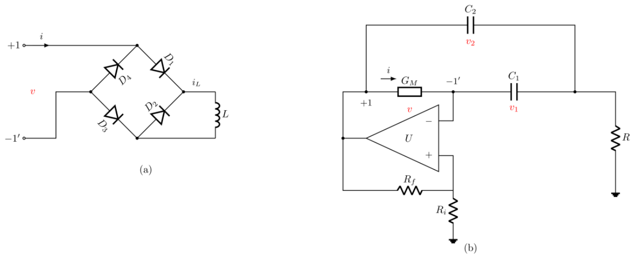
Figure 2.
Global organisation of the (a, k) plane over a ∈ [0.001, 0.08], k ∈ [0.02, 0.08]. (a,b) Two-parameter bifurcation maps for the negative and positive seeds. (c,d) Corresponding largest Lyapunov exponent fields for the two seeds; the zero-exponent contour marks the boundary between periodic and chaotic behaviour.
Figure 2.
Global organisation of the (a, k) plane over a ∈ [0.001, 0.08], k ∈ [0.02, 0.08]. (a,b) Two-parameter bifurcation maps for the negative and positive seeds. (c,d) Corresponding largest Lyapunov exponent fields for the two seeds; the zero-exponent contour marks the boundary between periodic and chaotic behaviour.
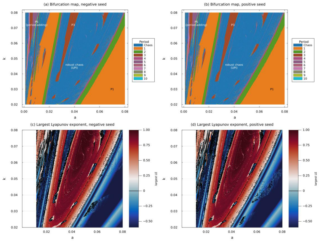
Figure 3.
Continuation-supported period-doubling loci (P1 → P2, solid; P2 → P4, dashed) overlaid on the largest Lyapunov exponent field. Each locus marks where a Floquet multiplier of the periodic orbit crosses the unit circle; the loci are shown over the range where they are single-valued.
Figure 3.
Continuation-supported period-doubling loci (P1 → P2, solid; P2 → P4, dashed) overlaid on the largest Lyapunov exponent field. Each locus marks where a Floquet multiplier of the periodic orbit crosses the unit circle; the loci are shown over the range where they are single-valued.
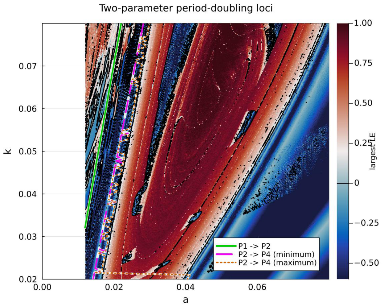
Figure 4.
Continuation-supported nominal route for k = 0.05; a = 0.002-0.08. (a,b) Negative- and positive-seed brute-force clouds overlaid with the continued P1-P4 branches of the corresponding coexisting family (subscripts 1 and 2), including the UPI-1 interval where the period-doubling skeleton persists only as unstable branches. (c,d) Corresponding largest Lyapunov exponent, with the zero line and representative operating points marked; MS marks the multistability check point at a = 0.0155.
Figure 4.
Continuation-supported nominal route for k = 0.05; a = 0.002-0.08. (a,b) Negative- and positive-seed brute-force clouds overlaid with the continued P1-P4 branches of the corresponding coexisting family (subscripts 1 and 2), including the UPI-1 interval where the period-doubling skeleton persists only as unstable branches. (c,d) Corresponding largest Lyapunov exponent, with the zero line and representative operating points marked; MS marks the multistability check point at a = 0.0155.
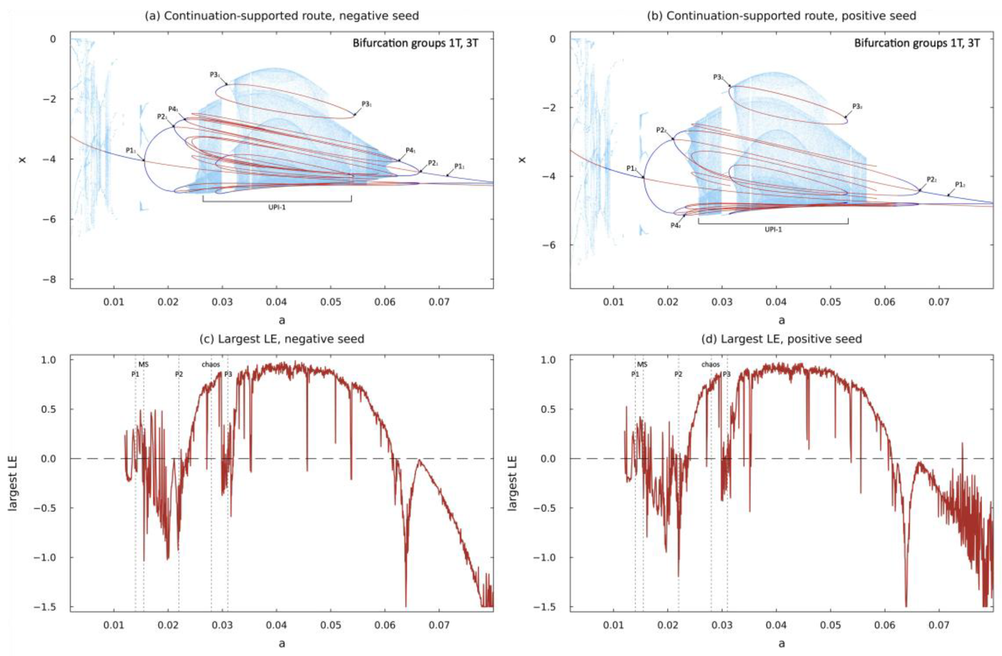
Figure 5.
Continuation-supported feedback-ratio cross-sections; k = 0.02-0.08. (a,b) a = 0.05 and (c,d) a = 0.06, for the negative and positive seeds. Each panel overlays the brute-force cloud with the continued branches of the coexisting instances — the doubling cascade P1₁ → P2₁ → P4₁, the lower sheet P1₂, P2₂, and the fully unstable P1₃ orbit between them — showing the cascade and its shift to larger k at larger capacitance. UPI-1 brackets mark candidate robust-chaos intervals — the longest without recovered stable low-period branches (Section 3.4).
Figure 5.
Continuation-supported feedback-ratio cross-sections; k = 0.02-0.08. (a,b) a = 0.05 and (c,d) a = 0.06, for the negative and positive seeds. Each panel overlays the brute-force cloud with the continued branches of the coexisting instances — the doubling cascade P1₁ → P2₁ → P4₁, the lower sheet P1₂, P2₂, and the fully unstable P1₃ orbit between them — showing the cascade and its shift to larger k at larger capacitance. UPI-1 brackets mark candidate robust-chaos intervals — the longest without recovered stable low-period branches (Section 3.4).
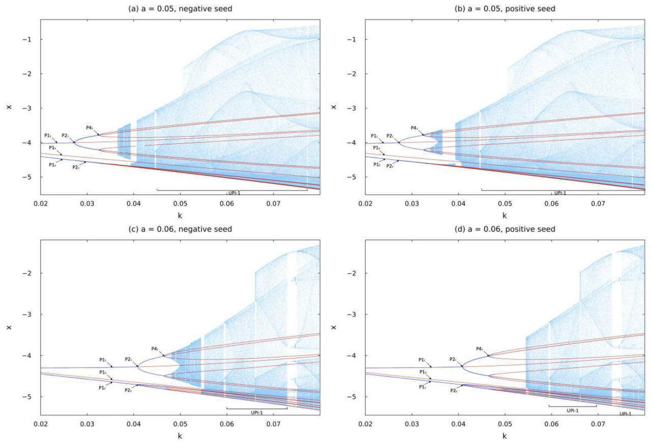
Figure 6.
Low-a higher-period window for k = 0.026. (a,b) Negative- and positive-seed two-parameter maps over the focused window. (c,d) Continuation-supported cross-sections aligned under the maps, showing the P4-centred branch structure of the negative-seed (subscript 1) and positive-seed (subscript 2) families, each with its unstable parent P1 branch continuing through the window.
Figure 6.
Low-a higher-period window for k = 0.026. (a,b) Negative- and positive-seed two-parameter maps over the focused window. (c,d) Continuation-supported cross-sections aligned under the maps, showing the P4-centred branch structure of the negative-seed (subscript 1) and positive-seed (subscript 2) families, each with its unstable parent P1 branch continuing through the window.
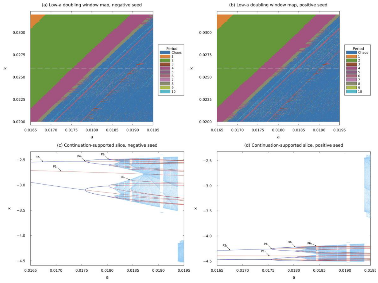
Figure 7.
Nominal mixed transition region for k = 0.05. (a,b) Negative- and positive-seed two-parameter maps showing the broad P3 window, the adjacent narrow P6 window, and nearby isolated higher-period islands. (c,d) Continuation-supported cross-sections with supported P3 and P6 branches; disconnected pieces denote locally recovered continuation support, and the P9 branch is retained only as a narrow local feature.
Figure 7.
Nominal mixed transition region for k = 0.05. (a,b) Negative- and positive-seed two-parameter maps showing the broad P3 window, the adjacent narrow P6 window, and nearby isolated higher-period islands. (c,d) Continuation-supported cross-sections with supported P3 and P6 branches; disconnected pieces denote locally recovered continuation support, and the P9 branch is retained only as a narrow local feature.
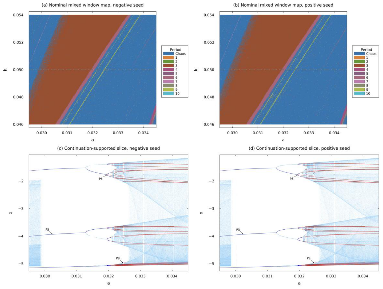
Figure 8.
High-a higher-period window for k = 0.044. (a,b) Negative- and positive-seed two-parameter maps. (c,d) Continuation-supported cross-sections showing the P4-centred branch structure of the negative-seed (subscript 1) and positive-seed (subscript 2) coexisting families, each with its unstable parent P1 branch threading the window; the parents regain stability beyond the plotted range.
Figure 8.
High-a higher-period window for k = 0.044. (a,b) Negative- and positive-seed two-parameter maps. (c,d) Continuation-supported cross-sections showing the P4-centred branch structure of the negative-seed (subscript 1) and positive-seed (subscript 2) coexisting families, each with its unstable parent P1 branch threading the window; the parents regain stability beyond the plotted range.
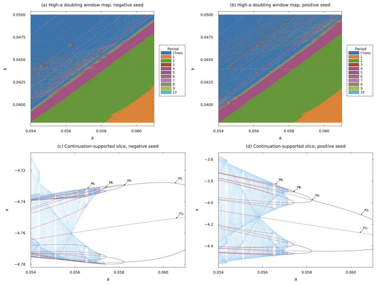
Figure 9.
Period-adding window for k = 0.078; a = 0.004-0.013. (a,b) Negative- and positive-seed two-parameter maps showing the period-5-dominated region with period-3, period-7, and period-9 substructure. (c,d) Continuation-supported cross-sections with P3, P5, and locally supported higher-period branches, illustrating the P3 → P5 period-adding transition.
Figure 9.
Period-adding window for k = 0.078; a = 0.004-0.013. (a,b) Negative- and positive-seed two-parameter maps showing the period-5-dominated region with period-3, period-7, and period-9 substructure. (c,d) Continuation-supported cross-sections with P3, P5, and locally supported higher-period branches, illustrating the P3 → P5 period-adding transition.
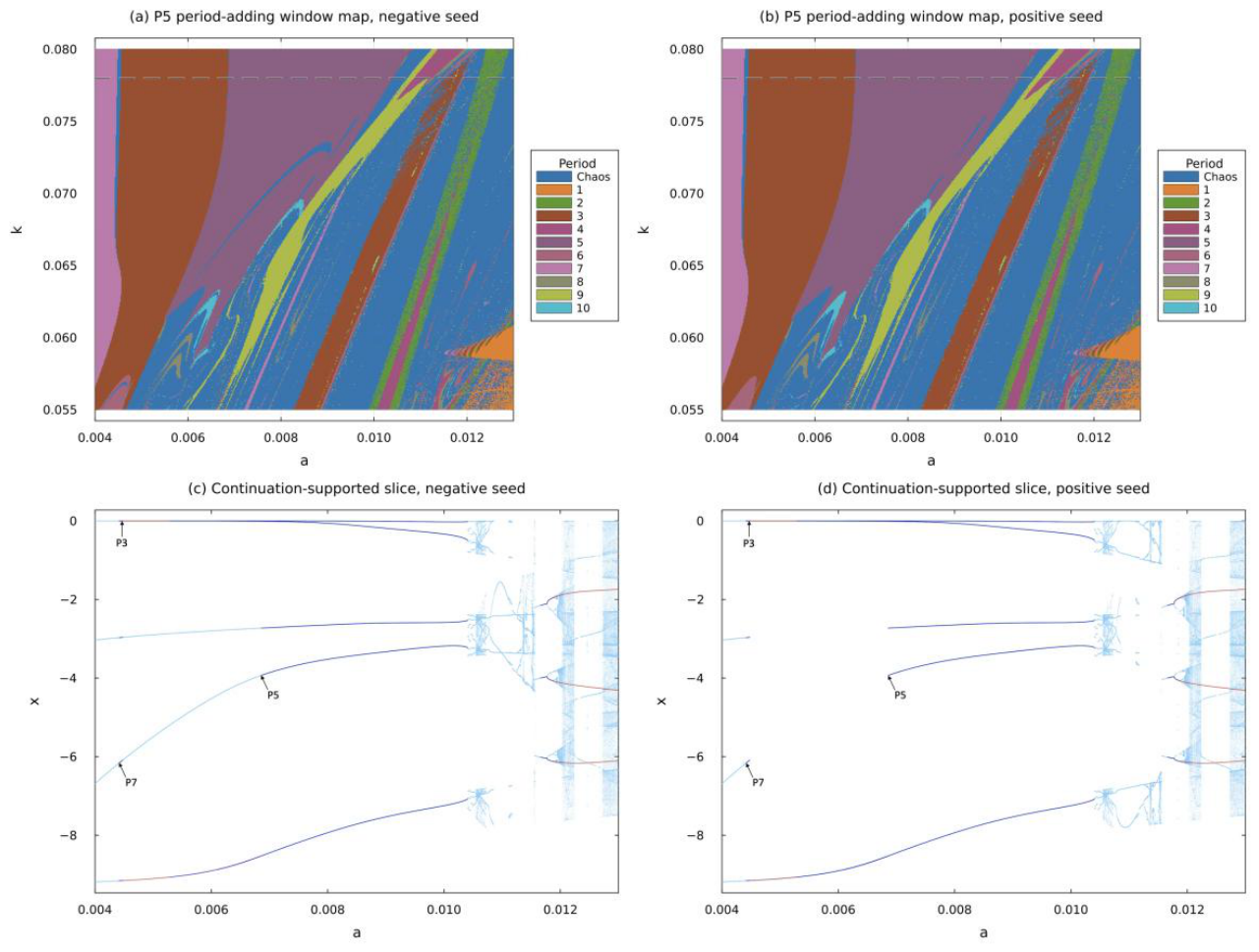
Figure 10.
Representative phase portraits in the (x, y) plane along the nominal slice k = 0.05: (a) P1 (a = 0.014), (b) P2 (a = 0.022), (c) chaotic (a = 0.028), and (d) P3 (a = 0.031).
Figure 10.
Representative phase portraits in the (x, y) plane along the nominal slice k = 0.05: (a) P1 (a = 0.014), (b) P2 (a = 0.022), (c) chaotic (a = 0.028), and (d) P3 (a = 0.031).
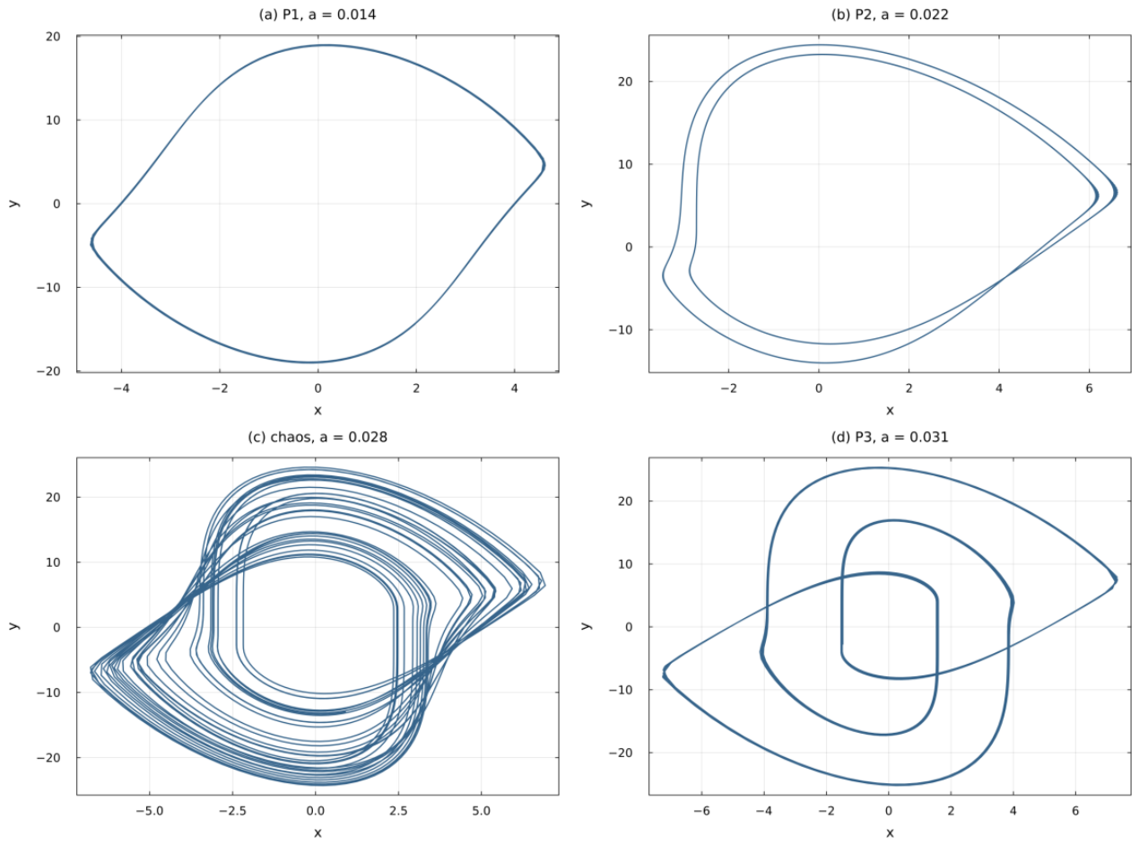
Figure 11.
Time series (a,c,e,g) and power spectra (b,d,f,h) of the P1, P2, chaotic, and P3 regimes at k = 0.05, showing discrete spectral combs for periodic regimes and a broadband spectrum for chaos.
Figure 11.
Time series (a,c,e,g) and power spectra (b,d,f,h) of the P1, P2, chaotic, and P3 regimes at k = 0.05, showing discrete spectral combs for periodic regimes and a broadband spectrum for chaos.
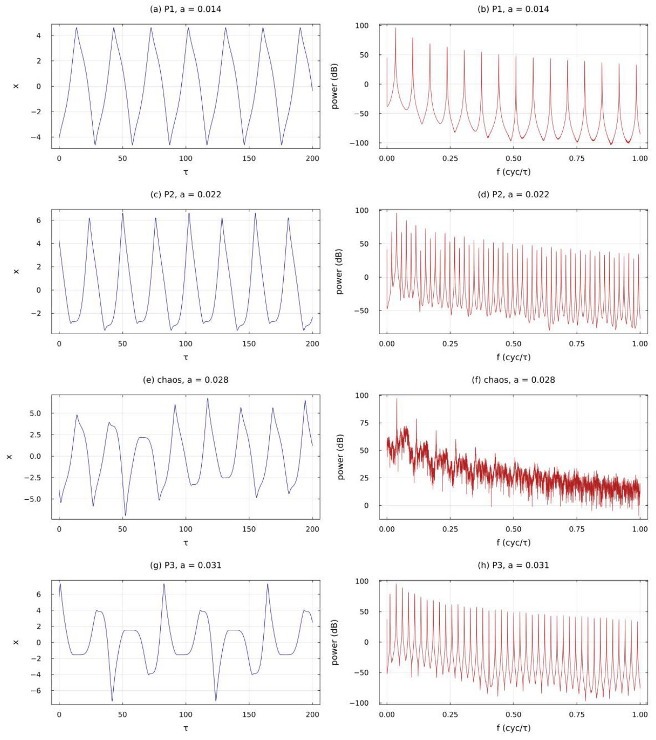
Figure 12.
Multistability at a = 0.0155, k = 0.05. (a) Basin of attraction in the (x0, z0) plane at fixed y0 = 0.01. (b) Overlaid coexisting P1 and P3 attractors with the P3 reflection partner.
Figure 12.
Multistability at a = 0.0155, k = 0.05. (a) Basin of attraction in the (x0, z0) plane at fixed y0 = 0.01. (b) Overlaid coexisting P1 and P3 attractors with the P3 reflection partner.
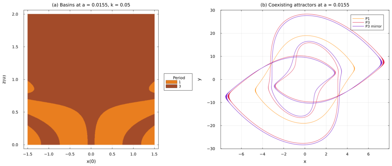
Figure 13.
Component-level ngspice phase portraits of the diode-bridge/op-amp circuit at k = 0.05, R = 50 Ω, Ri = 50 Ω, Rf = 1 kΩ, and L = 10 mH. The capacitance values were swept to recover the representative regimes in the nonideal circuit: (a) period-1 (C = 56 nF), (b) period-2 (C = 90 nF), (c) chaos (C = 105 nF), and (d) period-3 (C = 126 nF). Axes are the simulated capacitor voltages vC1 and vC2; compare with the ideal-model attractors of Figure 10 and the Xu et al. hardware sweep [7].
Figure 13.
Component-level ngspice phase portraits of the diode-bridge/op-amp circuit at k = 0.05, R = 50 Ω, Ri = 50 Ω, Rf = 1 kΩ, and L = 10 mH. The capacitance values were swept to recover the representative regimes in the nonideal circuit: (a) period-1 (C = 56 nF), (b) period-2 (C = 90 nF), (c) chaos (C = 105 nF), and (d) period-3 (C = 126 nF). Axes are the simulated capacitor voltages vC1 and vC2; compare with the ideal-model attractors of Figure 10 and the Xu et al. hardware sweep [7].
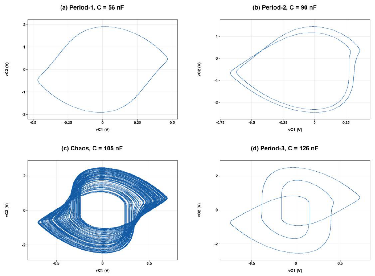
Figure 14.
Prototype board used for the hardware measurements: (a) component side; (b) trace side.
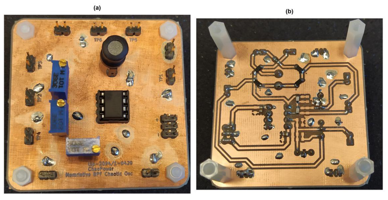
Figure 15.
Measured phase portraits in the (v1, v2) plane at R = 50 Ω, Ri = 50 Ω, L = 10 mH, ±10 V supply rails: (a) P1 (C = 100 nF, Rf = 1 kΩ); (b) P2 (C = 133 nF, Rf = 1 kΩ); (c) chaos (C = 100 nF, Rf = 232.3 Ω); (d) P3 (C = 100 nF, Rf = 472 Ω). Compare with the SPICE portraits of Figure 13.
Figure 15.
Measured phase portraits in the (v1, v2) plane at R = 50 Ω, Ri = 50 Ω, L = 10 mH, ±10 V supply rails: (a) P1 (C = 100 nF, Rf = 1 kΩ); (b) P2 (C = 133 nF, Rf = 1 kΩ); (c) chaos (C = 100 nF, Rf = 232.3 Ω); (d) P3 (C = 100 nF, Rf = 472 Ω). Compare with the SPICE portraits of Figure 13.
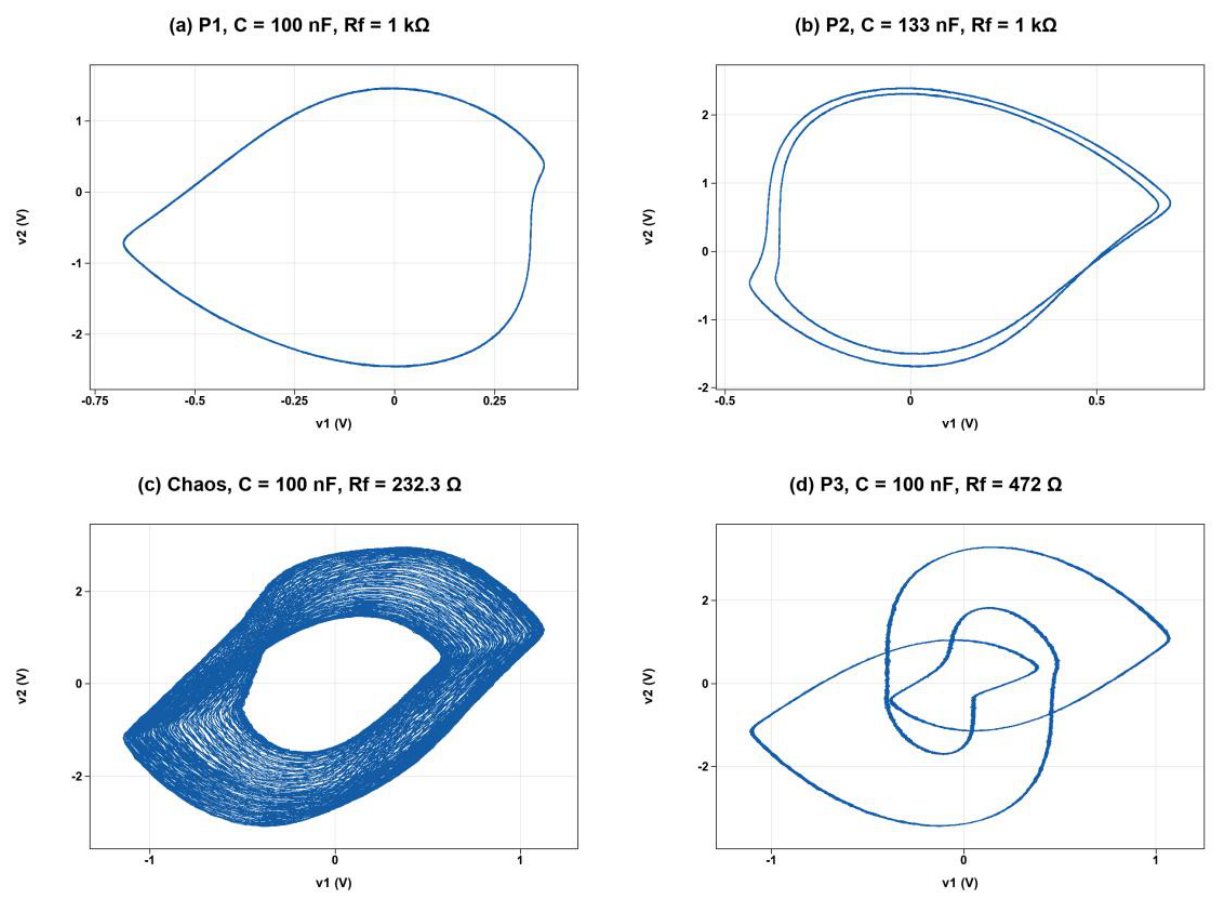
Figure 16.
Mode-transition graphs comparing hardware, SPICE, and model along the two measured routes. (a) Capacitance route at k = 0.05 (Rf = 1 kΩ); C = 4-320 nF. The hardware row marks the waveform-verified modes of the measured sweep (0.33-690 nF measured; points below 2 nF are omitted (Section 3.13), P1 continues to 690 nF, and 22 nF also carries a coexisting P4 attractor). The SPICE rows mark the component-level deck with the ideal (0.1 Ω) and lossy (45 Ω effective series resistance) inductor; the model rows give the interval classification of the two-parameter map line k = 0.05 for the two seeds, with windows narrower than 1 nF absorbed. The model P3 interval at C = 61.5-65.3 nF is the seed-reached member of the P1/P3 coexistence window of Section 3.10. (b) Feedback-ratio route at C = 100 nF; k = 0.04-0.28, with the corresponding Rf on the upper axis. The hardware row marks the measured trimmer settings (P4 is the period-4 candidate at 407 Ω, P11 the period-11 locking at 270 Ω; the P1 at 150 Ω lies beyond the plotted range); the SPICE rows mark the ideal- and lossy-inductor decks swept in Rf; the model rows give brute-force/Lyapunov cross-section classifications at the nominal a = 0.025 and the boundary-matched effective a = 0.0195 (negative seed shown), with windows narrower than 0.002 in k absorbed.
Figure 16.
Mode-transition graphs comparing hardware, SPICE, and model along the two measured routes. (a) Capacitance route at k = 0.05 (Rf = 1 kΩ); C = 4-320 nF. The hardware row marks the waveform-verified modes of the measured sweep (0.33-690 nF measured; points below 2 nF are omitted (Section 3.13), P1 continues to 690 nF, and 22 nF also carries a coexisting P4 attractor). The SPICE rows mark the component-level deck with the ideal (0.1 Ω) and lossy (45 Ω effective series resistance) inductor; the model rows give the interval classification of the two-parameter map line k = 0.05 for the two seeds, with windows narrower than 1 nF absorbed. The model P3 interval at C = 61.5-65.3 nF is the seed-reached member of the P1/P3 coexistence window of Section 3.10. (b) Feedback-ratio route at C = 100 nF; k = 0.04-0.28, with the corresponding Rf on the upper axis. The hardware row marks the measured trimmer settings (P4 is the period-4 candidate at 407 Ω, P11 the period-11 locking at 270 Ω; the P1 at 150 Ω lies beyond the plotted range); the SPICE rows mark the ideal- and lossy-inductor decks swept in Rf; the model rows give brute-force/Lyapunov cross-section classifications at the nominal a = 0.025 and the boundary-matched effective a = 0.0195 (negative seed shown), with windows narrower than 0.002 in k absorbed.
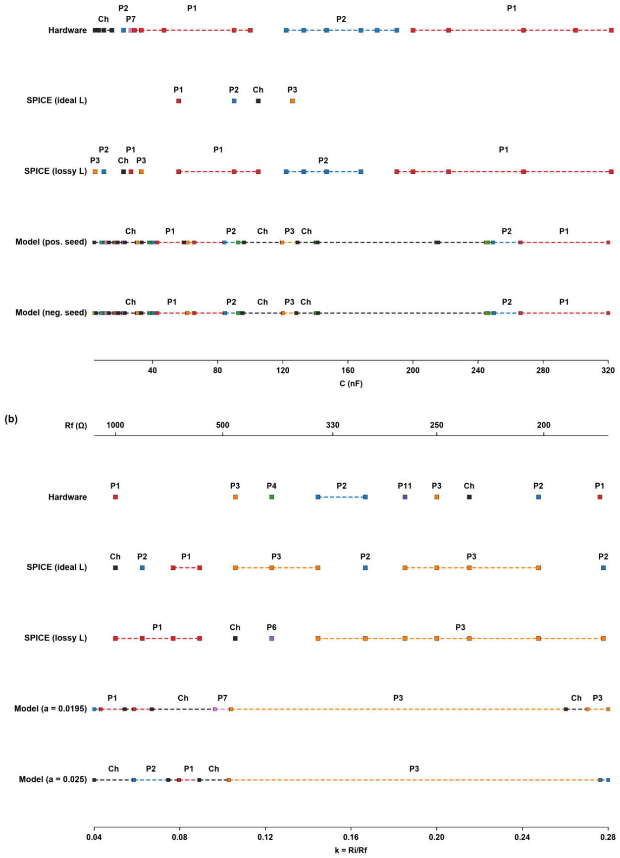

Table 1.
Numerical settings used to generate figures. Where a setting varies between the global and focused passes, both values are given.
Table 1.
Numerical settings used to generate figures. Where a setting varies between the global and focused passes, both values are given.
| Quantity | Setting |
|---|---|
| Two-parameter period maps (grid in a × k) | 1001 × 1001 (global plane); 501 × 501 (focused window maps) |
| Largest Lyapunov exponent fields (grid in a × k) | 500 × 500 |
| One-parameter cross-sections (samples in the swept parameter) | ≈ 2000 brute-force parameter values; ≈ 2000 Lyapunov samples |
| Poincaré section | hyperplane y = 0, upward crossings, projected to (x, z) |
| Return iterations retained per map cell | 130 (period maps); up to 300 (Lyapunov fields) |
| Return iterations per brute-force cross-section point | 800 computed, first 300 discarded as transient (500 retained) |
| Period-detection tolerance / maximum period | 10-3 / 10 |
| Lyapunov method | two-trajectory (Wolf) on the return map, renormalised at every return crossing |
| Lyapunov perturbation size δ₀ | 10-8 |
| Chaos/periodic threshold (neutral tolerance) | largest exponent > 10-3 classified chaotic; exponents at or below the threshold classified periodic/neutral |
| Continuation method | pseudo-arclength (PALC) of the Poincaré return map |
| Continuation step ds / dsmax / dsmin | 2.5 × 10⁻⁵-1 × 10⁻⁴ / 1.25 × 10⁻⁴-8 × 10⁻⁴ / 10-8 |
| Newton corrector tolerance / max iterations | 10-8 (10-7 for the refined nominal-route pass) / 30-70 |
| Maximum continuation steps per branch | 350-3500 |
| Bifurcation / stability criterion | Floquet multiplier μ of the return map: fold at μ = +1, period-doubling at μ = −1; stable if the multiplier modulus is ≤ 1 |
| ODE solver / tolerances | AutoTsit5(Rosenbrock23()) / reltol = abstol = 10-8 |
| Initial-condition seeds | (x, y, z) = (0, ±0.01, 0) (positive / negative) |
Table 2.
Practical operating guidance derived from the two-parameter map and continuation-supported cross-sections.
Table 2.
Practical operating guidance derived from the two-parameter map and continuation-supported cross-sections.
| Purpose / regime | Parameter window | Approximate component setting | Expected response | Recommendation |
|---|---|---|---|---|
| Nominal low-period reference | k = 0.05, a = 0.014 or 0.022 | C ≈ 56 nF (P1) or 88 nF (P2) for L = 10 mH; Ri/Rf = 0.05 | Stable periodic oscillation | Useful for calibration and model comparison, not for chaos generation. |
| Primary robust-chaos candidate band | k = 0.05, a ≈ 0.033-0.055; preferred interior a ≈ 0.04-0.05 | C ≈ 132-220 nF; preferred C ≈ 160-200 nF for L = 10 mH; Ri/Rf = 0.05 | Broad positive-Lyapunov chaotic band | Preferred candidate chaos-source region; choose an interior point away from the P3 edge and high-a periodic windows, and observe the damping limit below; the interior anchors are census-checked for coexisting attractors (Section 3.1). |
| Memristor-branch damping limit | any robust-chaos set point | inductor DC plus AC series resistance below ≈ 10-20 Ω for the L = 10 mH emulator | chaos collapses through a reverse period-doubling to P2/P1 by ≈ 30-45 Ω | Measure the inductor's effective series resistance before selecting chaos set points (Section 3.13). |
| Fixed-capacitance k-route into chaos | a = 0.05-0.06; P1 → P2 begins near k ≈ 0.027 / 0.041, and the P2 → P4 threshold lies near k ≈ 0.033 / 0.047 | C ≈ 200-240 nF for L = 10 mH; raise Ri/Rf from the low-period side toward the high-k chaotic side | P1 → P2 → P4 → chaos cascade | Use k as a resistor-set tuning knob; avoid operating close to the continuation-traced doubling thresholds. |
| Component-SPICE validation anchors | k = 0.05, L = 10 mH, nonideal diode/op-amp deck | C = 56, 90, 105, 126 nF for P1, P2, chaos, P3 | Same qualitative sequence in the realisable circuit, close to the Xu hardware sweep | Use as the first hardware-validation sweep; retune around these values for actual devices. |
| Symmetry-organised multistability | k = 0.05, a ≈ 0.0155 | C ≈ 62 nF for L = 10 mH; Ri/Rf = 0.05 | Coexisting P1 and mirror-related P3 attractors | Avoid for robust chaos; useful only if initial-condition-controlled mode selection is desired. |
| Narrow higher-period windows | Low-a P4 near a ≈ 0.0176-0.0180, nominal P6 near a ≈ 0.0320, high-a P4 near a ≈ 0.0574-0.0582 | C ≈ 70-72 nF, ≈128 nF, or ≈230-233 nF for L = 10 mH, with the corresponding k slices of Figure 6, Figure 7 and Figure 8 | Periodic or locally mixed windows embedded near chaotic regions | Avoid as chaos-source set points because small drift can switch the response. |
| Low-a, high-k period-adding window | k ≈ 0.078, a ≈ 0.0069-0.0104 | C ≈ 28-42 nF for L = 10 mH; Ri/Rf ≈ 0.078 | Stable P5 family with P7/P9 substructure | Scientifically useful period-adding target; not the recommended robust-chaos operating band. |
Disclaimer/Publisher’s Note: The statements, opinions and data contained in all publications are solely those of the individual author(s) and contributor(s) and not of MDPI and/or the editor(s). MDPI and/or the editor(s) disclaim responsibility for any injury to people or property resulting from any ideas, methods, instructions or products referred to in the content. |
© 2026 by the authors. Licensee MDPI, Basel, Switzerland. This article is an open access article distributed under the terms and conditions of the Creative Commons Attribution (CC BY) license (http://creativecommons.org/licenses/by/4.0/).
Copyright: This open access article is published under a Creative Commons CC BY 4.0 license, which permit the free download, distribution, and reuse, provided that the author and preprint are cited in any reuse.


