

Submitted:
13 July 2026
Posted:
15 July 2026
You are already at the latest version
Abstract
Deterministic AI weather and ocean models are far more computationally efficient and achieve lower mean-square error than state-of-the-art operational forecasts, yet they are widely criticized for violating physical constraints, smoothing small scales, and underestimating extremes. We offer a unified Markov-process explanation: MSE-trained deterministic models learn the conditional mean E[x_{t+Δt} | x_t] rather than the full transition law P(x_{t+Δt} | x_t). This mean-field limit links low RMSE to poor conservation, spectral dissipation, and weak extremes. We support the theory with a finite-state Markov experiment and a stochastically perturbed Kelvin-Helmholtz fluid experiment using matched U-Net backbones. From an information-entropy perspective, deterministic forecasts are low-entropy and overconfident relative to atmospheric and oceanic variability, whereas diffusion models sample from conditional transition distributions and better match intrinsic complexity. Distributional generative forecasting may therefore be better suited to future AI prediction, reconstruction, and bias correction.
Keywords:
AI weather forecasting
; probabilistic mean field
; deterministic forecasting
; extreme event
; physical unconservation
Key Points
- Under the Markov Process assumption, we declare that for existing deterministic AI weather forecasting models optimized with RMSE as the objective function, the optimal weight parameters obtained by minimizing this objective imply that each forecast is the conditional expectation , which we refer to as the probabilistic mean field.
- Drawing on mathematical analysis and two experiments exploring the averaging property of the probabilistic mean field , we elucidate three major limitations encountered in deterministic AI weather forecasting models: insufficient physical conservation, high-frequency power dissipation, and poor extreme-value prediction.
- We further show that deterministic forecasting models, regardless of RMSE, MAE, or related regression losses, produce a systematic information-entropy mismatch with the true future field, reflecting overconfidence in every prediction. Conditional generative models such as GANs and diffusion models, which learn , instead produce probabilistic forecasts and provide a distribution-aware alternative that may mitigate the three deterministic deficiencies identified above.
Plain Language Summary
AI weather and ocean models are much faster than traditional forecast models and often have low average error. But they can also look too smooth, miss extreme events, and fail to follow basic physical rules. We explain this with a simple idea: when AI models are trained to minimize average error, they learn a weighted average over all possible outcome, not the full range of possible futures. That typical forecast is smoother and less extreme than reality. We test this idea in two experiments: a simple probability model and a turbulent fluid-flow model. In both cases, average-error models look good in error scores but miss real variability. Diffusion models, which can generate multiple possible futures, better match realistic small-scale structure. This suggests that the main problem is not one training choice, but deterministic forecasting itself. Future AI systems may work better if they forecast distributions, not just a single best guess.
1. Introduction
Since the advent of AI weather models epitomized by Pangu-Weather [1], a wide range of AI forecasting systems for meteorology and oceanography have sprung up globally [2,3,4,5]. Several of these AI model can intermittently surpass conventional state-of-the-art physics-based numerical weather prediction (NWP) systems in forecast accuracy, alongside prominent superiority in computational speed and energy consumption efficiency [6]. Accordingly, they are increasingly deployed to provide rapid, operationally scalable global forecast support for disaster risk reduction, renewable energy scheduling, heavy-precipitation-related hazards and marine activities and coastal management [3,4,7,8,9].
Nevertheless, AI weather models still suffer from notable limitations, including overly smoothed forecast , systematic underestimation of extreme events and violation of physical conservation laws [1,8,10]. For instance, Pangu-Weather tends to produce smoother contour lines and predicts similar values for neighboring grid points, which is considered as an inherent property of deep neural networks. In contrast, traditional operational NWP systems (IFS) better preserve small-scale structures, even though yielding inferior overall performance in terms of RMSE and ACC [1]. A clear example is Storm Ciarán, during which leading AI models captured the cyclone track and large-scale structure well but underestimated peak 10-m wind speeds by roughly 8-9 m relative to IFS and failed to reproduce sharp frontal gradients essential for warning issuance [11]. For flood-relevant precipitation, the catastrophic North China event exposed a complementary limitation: standalone AI global forecasts struggle to resolve mesoscale rainfall maxima and sharp accumulation gradients that drive hydrological impacts, even when large-scale patterns are broadly captured [12]. Complementary diagnostics from ECMWF indicate that such deficits are part of a broader pattern in data-driven models: even at short forecast lead times, Pangu-Weather exhibits pronounced spectral damping for wavenumbers above approximately 60, corresponding to spatial wavelengths shorter than roughly 700 km, relative to physics-based ensemble forecasts, yielding systematically smoother fields than observed [8]. Moreover, the predicted wind and mass fields become progressively less dynamically consistent with one another as forecast lead time increases, manifesting as a growing departure from geostrophic balance. Spectral budget analyses further show that Pangu-Weather underestimates mesoscale kinetic energy and fails to maintain the canonical mesoscale energy cascade seen in physics-based models [13]. This physical unconservation phenomenon is not limited to Pangu-Weather as a special case. Further investigation on the FuXi weather model that AI Weather forecast model violates global dry-air-mass, moisture-budget, and energy conservation [14] .
Existing views generally attribute these weakness to a hierarchy of mechanisms in current data-driven forecasting. At the most fundamental level, mainstream AI weather models do not embed atmospheric governing equations and instead learn mappings directly from historical reanalysis data [1,10]. Their forecasts therefore depend primarily on statistical interpolation within the learned state space rather than on physical extrapolation, which first limits skill for out-of-distribution extremes and maintain physical conservation. This extrapolation weakness is further amplified by the rarity of extreme events in training datasets, a classic data imbalance problem that biases optimization toward common weather states and contributes to systematic underestimation of both extreme intensity and occurrence frequency [10,15]. Additionally, from the perspective of the frequency principle (F-principle), deep networks tend to fit low-frequency components before high-frequency details, making fine-scale structures difficult to learn fully and providing an additional explanation for the attenuation of small-scale variability and extreme amplitudes [16].
Although the aforementioned interpretations have deepened our understanding of weakness in artificial intelligence forecasting, most of these explanations are merely phenomenological. They fail to establish a unified theoretical framework that can comprehensively account for three key issues of AI weather models: insufficient physical conservation, dissipation of high-frequency power spectra, and inadequate capability in extreme value prediction. Inspired by the “double penalty” effect [17,18], where a misplaced forecast is penalized both for missing the observed feature and for producing spurious structure at the wrong location, and where squared errors more broadly favor smooth predictions, we further declare that deterministic forecast models with MSE-type loss are effectively trained to recover the conditional mean field rather than its full probabilistic structure [19]. This mean-seeking behavior offers a common theoretical basis for understanding why such models may achieve competitive bulk errors while still failing to preserve conservation constraints, maintain high-frequency variance, and represent extremes.
As shown in Figure 1, panel A(i) illustrates the bimodal case that when is non-Gaussian, the conditional expectation may fall in a low probability region between modes rather than near either mode. Panel A(ii) illustrates the long-tail case that tails can place far from rare extremes, so a single conditional mean offers little predictive value for extreme events. Panel B provides a non-intuitive geometric view: the green samples lie on a convex manifold that schematically represents admissible physical states, yet the Euclidean mean of any n such points need not remain on ; a mean-based forecast can therefore be not only statistically unrepresentative but also physically inadmissible. Contrary to the conventional intuition that minimizing RMSE can continuously narrow the gap between predictions and targets while satisfying physical conservation constraints, we elaborate that pursuing the lowest RMSE in deterministic AI models will instead lead to physical non-conservation. This finding may inspire the reassessment of existing meteorological AI forecasting models or the reconstruction of evaluation paradigms for such models in future research.
The remainder of this paper is organized as follows. Section 2 develops the theoretical basis of this study. We model atmospheric and oceanic evolution as a discrete-time stochastic Markov process and show that deterministic AI models trained with RMSE learn the conditional mean rather than the full transition law . We further explain why this probabilistic mean field underestimates extremes and high-frequency variability, and show that it is generally not a solution of the original nonlinear governing equations, so physical non-conservation may be a structural consequence of RMSE-optimal deterministic forecasting. Section 3 presents the experimental design used to validate the theory in Section 2. We learn an Markov transition matrix with two MLP neural networks: one trained with RMSE to predict a scalar next state, and one trained with cross-entropy to predict the full conditional distribution. This section further represents a 200-member stochastically perturbed Kelvin–Helmholtz Trixi ensemble to compare two one-step forecasters on four-channel states: a U-Net [20] trained with RMSE to predict the conditional-mean next state, and an EDM diffusion model [21] by comparison with the same U-Net backbone trained to sample from the conditional next-state distribution [22,23]. Section 4 reports the experimental results and related quantitative analyses. Section 5 discusses the main findings, highlights development trend of AI forecasting models, and concludes the paper.
2. Preliminaries
2.1. Markov Formulation Of Atmospheric And Oceanic Forecasting
Atmospheric and oceanic evolution can be approximated as a discrete-time Markov process [24,25,26]. Let the system state at time t be denoted by , where represents the joint phase space of atmospheric and oceanic variables (e.g., temperature, winds, pressure, sea surface height, and related fields on a model grid). The one-step transition law is written as
which states that the future depends on the past only through the present state. Equivalently, the conditional transition probability density is
As in contemporary data-driven meteorological models, the forecast is produced by a deterministic neural network whose parameters are learned from historical state pairs. Given a training set , the model parameters are updated by backpropagation to minimize the empirical MSE as the primary objective:
2.2. Mse Minimization Yields The Conditional Mean
Proposition 1
(MSE-optimal deterministic forecast as conditional expectation). Let be generated by the Markov process (1)–(2), and assume . Consider any measurable estimator and define the population MSE risk
Then any minimizer of satisfies
Proposition 1 shows that deterministic models trained with RMSE recover the conditional mean . They do not, in general, recover the full conditional distribution . Therefore, low RMSE does not imply that the model has learned the complete Markov transition law in (2). Consequently, such models have limited skill for rare, abrupt extremes and tend to underestimate both the frequency and intensity of low- and high-quantile events.
Proposition 2
(Conditional expectation is not a nonlinear physical solution). Let be a random state generated by a nonlinear dynamical system
where is nonlinear. Suppose every sample path satisfies this equation, and define the one-step conditional mean
If the conditional distribution of given is not almost surely degenerate, then is not, in general, a solution of . Instead,
Moreover, whenever is non-affine on the support of the conditional distribution. A detailed proof is provided in the Supplementary Information (SI).
Proposition 2 shows that a conditional-mean forecast need not satisfy the underlying nonlinear dynamics. The resulting behavior is counter-intuitive: the more aggressively a model is optimized for lower RMSE, the more it may converge to a statistically optimal yet physically non-realizable mean field, with degraded representation of physical constraint-preserving structure.
3. Data and Methods
3.1. Markov Transition-Matrix Experiment
To validate Proposition 1 in a controlled setting, we design a toy experiment in which the underlying atmospheric or oceanic evolution is represented by a finite-state Markov chain. The state space is , with . For each experiment, the scalar states are placed uniformly on :
The one-step transition law is a row-stochastic matrix , with entries
Each row of P is drawn independently from a symmetric Dirichlet distribution, , with and random seed fixed at 0. This construction yields a random but unbiased transition matrix without hand-crafted multi-modal structure.
Training pairs are generated by simulating the Markov chain. For each current state index i, we sample next states from and construct a dataset of state transitions. We use 100,000 transition pairs for and , and 500,000 pairs for . The data are split into 80% training and 20% testing subsets. Sampling is balanced across current states so that each row of P is equally represented during optimization. Two multilayer perceptrons (MLPs) are trained on the same transition dataset. The first model, denoted MLP(RMSE), represents the deterministic regression strategy used in operational AI weather models. It takes the current scalar state as input and outputs a scalar prediction , trained to minimize the mean squared error (MSE). The second model, denoted MLP(Cross-Entropy), represents explicit distributional learning of the transition law. It takes a one-hot encoding of the current state index as input and outputs a K-dimensional logit vector.
To compare the learned transition law with the true matrix P, we construct an inferred transition matrix from each model. For MLP(Cross-Entropy), row i is taken directly as the predicted probability vector. For MLP(RMSE), row i is reconstructed from the scalar prediction by mapping to the nearest grid state:
This nearest-state reconstruction reflects the fact that a scalar regression model cannot represent a full probability vector. Detailed experimental configurations are provided in SI Table S1.
3.2. Kelvin–Helmholtz Experiment: Probabilistic vs. Deterministic Forecasting
The second experiment extends the theoretical result in Section 2 from discrete-state Markov chains to a spatially extended fluid system. Our objective is to systematically compare the forecasting behaviors of deterministic and probabilistic AI models from mainstream but distinct forecasting frameworks. Because diffusion-based generative models are trained to represent a target distribution rather than a single point forecast, we expect them to learn the conditional transition law more faithfully than mean-seeking deterministic models. Following GenCast [27], we adopt its diffusion-based ensemble approach and compare it with the deterministic conditional-mean output of Pangu [1]. We study this question using the two-dimensional (2D) compressible Kelvin–Helmholtz (KH) instability as a prototype chaotic flow [28]. The governing equations are the 2D compressible Euler equations on a periodic domain :
where is the vector of conserved variables, is density, is velocity, E is specific total energy, and is the corresponding flux tensor for an ideal gas with ratio of specific heats . In primitive form, the prognostic fields are , where p is pressure. The KH setup consists of a tanh shear layer with a sinusoidal cross-stream perturbation, which triggers roll-up of the shear interface and growth of multiscale structure.
To represent the atmospheric and oceanic forecasting problem as a Markov process, we do not integrate a single deterministic trajectory. Instead, we generate an ensemble of conditionally independent trajectories that share the same baseline initial condition but diverge through per-step random perturbations. Let denote the state of ensemble member m at time t. Conceptually, the evolution can be written as
where is the deterministic numerical time-step operator and is a member-specific random perturbation. In practice, after each accepted time step of the numerical solver, we add a multiplicative Gaussian perturbation to every conserved variable:
with relative amplitude . All members use the same initial-condition seed, while member m uses perturbation seed . This design keeps the large-scale initial structure identical across members while allowing the transition law to be broadened by unresolved stochastic variability. The resulting ensemble therefore provides a Monte Carlo approximation of the conditional distribution of future states.
Numerically, Equation (13) is solved with the Trixi DGSEM solver on an adaptively refined mesh (polynomial degree , base refinement level 5, AMR enabled). We integrate each member from to and save snapshots every . In total, we run 200 ensemble members. Some members terminate before owing to numerical instability; for those members we retain all frames produced before failure. Each saved snapshot is exported on a uniform grid covering , with four channels . Member m is thus represented by a sequence
where is the number of saved frames for that member.
On the KH dataset, we compare two one-step U-Net forecasters with identical backbones (): a deterministic model trained with global RMSE loss, , and a probabilistic EDM diffusion model trained to sample from the conditional law . At inference, both models are rolled out autoregressively from the ground-truth initial state, with , yielding a deterministic nonlinear Markov surrogate in the RMSE case and an ensemble of stochastic trajectories in the diffusion case. We split the 200 ensemble members into 180 training and 20 test trajectories , reserving 10 training members for validation and early stopping. All consecutive pairs from the training pool are used to compute channel-wise normalization statistics.
4. Results and Discussion
4.1. Markov Transition-Matrix Results
Figure 2 compares the true transition matrix with the matrices inferred by MLP under two training objectives: continuous next-pixel value regression optimized with RMSE loss, and discrete pixel category prediction using softmax output paired with cross-entropy loss, for , , and . For each case, the left panel shows the randomly generated ground-truth matrix P, the middle panel shows the matrix reconstructed from the RMSE-trained scalar model, and the right panel shows the matrix learned by the cross-entropy model.
Across all three state dimensions, the two models achieve nearly identical RMSE on the test set (Table 1). For example, at , the RMSE values are 0.579 for MLP (RMSE) and 0.577 for MLP(Cross-Entropy). This indicates that both models recover the conditional mean with similar point-wise accuracy. However, the distributional fidelity differs sharply. The KL divergence between the true and inferred transition matrices remains large for MLP(RMSE) at all scales: 8.38 for , 14.81 for , and 14.06 for . In contrast, MLP(Cross-Entropy) achieves KL values near zero: 0.0002, 0.0016, and 0.0170 for the same three cases. The RMSE-trained model therefore approximates the row-wise conditional means well, but fails to recover the full transition law . As shown in the middle panels of Figure 2, the inferred RMSE matrix collapses each row to a single nearest grid state, producing an effectively one-hot and overly concentrated transition matrix. The Cross-Entropy model, by contrast, reproduces the spread, multi-modality, and tail structure of the true transition rows.
Moreover, because RMSE training targets the conditional expectation, the scalar outputs , , and converge to approximately , , and respectively. None of these values coincide with any legal state in . This mismatch is analogous to the familiar property of nonlinear dynamics that a linear superposition of admissible solutions need not remain admissible: compressing a genuine transition distribution to its mean yields a point that may lie outside the discrete state space and cannot represent the original Markov kernel.
These results provide direct numerical support for the theoretical distinction established in Section 2. Minimizing RMSE leads to learning , not the full conditional distribution. A model can therefore appear accurate in RMSE while remaining a poor representation of the underlying Markov transition law.In the subsequent discussion, we further interpret this failure from the standpoint of entropy reduction. Deterministic RMSE regression effectively compresses the conditional transition distribution into a single-point prediction, thereby collapsing stochastic uncertainty and simplifying the intrinsic complexity of the underlying dynamical system. For a transition row , the Shannon entropy is
which measures the intrinsic uncertainty in the one-step transition law [29]. RMSE training replaces by an effectively degenerate law supported on a single predicted value, so that the distributional entropy is driven toward zero even when in the true Markov system.
4.2. Kelvin–Helmholtz Experiment: Deterministic Mean Vs. Diffusion Samples
We train two one-step forecasters on Kelvin–Helmholtz (KH) fields for under matched experimental conditions: the same dataset, the same U-Net backbone width (base_ch=32), and the same training configs. The deterministic model minimizes mean squared error (MSE) and predicts a single map ; the diffusion model uses the same U-Net as its denoiser and learns a conditional distribution via EDM, from which we draw stochastic rollouts. Both models are trained to convergence; and validation RMSE is summarized in SI Table S2. The deterministic U-Net attains a slightly lower validation RMSE (0.0904) than the EDM U-Net (0.1089).The slightly lower validation RMSE of Det U-Net is therefore not a contradiction of the spectral and structural contrasts discussed below. Rather, it anticipates them: although pointwise error is smaller, the deterministic mean field is smoother, dissipates more high-k power, and loses fine-scale detail relative to truth and to diffusion samples. More importantly, diffusion models can provide reliable probabilistic forecasts: the spread of an generated ensemble is well correlated with the actual forecast error. Deterministic models cannot offer this property, because they produce a single map rather than a calibrated predictive distribution.
Figure 3 shows, for as a representative example, a test-set trajectory in which every model is initialized from the same ground-truth state. At early times ( to ), both forecasts remain close to the truth. After several autoregressive steps ( to ), the deterministic field turns noticeably smoother: small vortical structures and sharp gradients are weakened, while individual diffusion samples still show fine-scale turbulent features. This difference does not appear only at the first forecast step; it grows and remains visible late in the rollout.
As KH evolution is controlled by shear-layer rotation, an important physcial conservation diagnositc variable is vorcity (). We diagnose the time-mean domain vorticity RMSE, , between each rollout and the Truth reference. As shown in SI Table S3, Det U-Net and EDM U-Net exhibit different fidelity to the rotational dynamics of Kelvin–Helmholtz (KH) instability. Exemplified by four randomly selected test members, members 14, 31, and 137 of EDM diffusion members achieve lower than Det U-Net, whereas member 3 provides a contrasting case in which the deterministic rollout is slightly better. This pattern indicates that stochastic diffusion samples can better represent rotational KH structure than a single conditional-mean trajectory.
Another physical-conservation diagnostic targets the domain-integrated x-momentum on the same periodic Kelvin–Helmholtz rollouts. Because the reference simulation is unforced and periodic, should remain nearly constant in time; we therefore measure the end-of-rollout percent drift and report the bulk consistency error , which quantifies how closely a predicted rollout preserves the global x-momentum budget of the Truth reference. As shown in SI Table S4, all EDM samples yields smaller than Det U-Net, with reductions of best samples ranging from 26.5% to 99.1%. Det U-Net systematically produces spurious positive of order –, whereas the Truth reference remains within and representative EDM samples track the reference drift to within . These results indicate that EDM U-Net better preserves bulk x-momentum consistency than Det U-Net.
While probes global integral behavior, it does not characterize whether fine-scale variability is retained or overly smoothed. To quantify multi-scale fidelity, we also examine the radial power spectrum, a standard diagnostic for small-scale structure and a useful proxy for whether a model preserves physical conservative. Figure 4 compares radial power spectra averaged over five held-out test members at and . We focus on these late times because the flow has become strongly nonlinear and less predictable, and because the truth develops pronounced high-frequency structure that is most difficult to preserve in autoregressive forecasting. At low wavenumbers (), all methods remain close to the reference. However, at higher wavenumbers( ), the deterministic U-Net exhibits pronounced spectral dissipation: its power falls far below the truth, indicating loss of sub-grid detail and sharp gradients. Individual diffusion trajectories, by contrast, remain much closer to the reference spectrum over the same rollout horizon, consistent with the visual sharpness in Figure 3.
These two views support the Markov argument developed in Section 2: MSE training targets the conditional expectation , which is smooth whenever the conditional distribution is broad or multi-modal. Diffusion sampling approximates draws from and can represent small-scale variability that the mean field suppresses. We further test this interpretation with a ten-member diffusion ensemble per initial condition. Let denote independent EDM rollouts sharing the same . The ensemble mean
should coincide, in principle, with the MSE deterministic prediction when both models are well trained on the same data. This is exactly what we observe: in Figure 3, (EDM U-Net mean) is visually similar to the deterministic field (Det U-Net) and both are smoother than the truth and than any single sample. In Figure 4, the ensemble-mean spectrum nearly overlaps that of the deterministic U-Net and lies well below the truth at high k, while each individual diffusion member tracks the reference much more closely. In other words, the deterministic model performs well in mean-square error because it approximates the conditional mean, not because it fully captures the transition distribution. Individual diffusion samples better represent small-scale structure, while their ensemble mean again resembles the deterministic forecast and shows a similar high-k spectral deficit.
Recent AI weather and ocean models often train with MSE-type objectives, but many also employ MAE losses or other related variants. In this study we use MSE alone in both the Markov analysis and the KH experiments, mainly for clarity and direct comparison with the conditional-mean theory. This choice should not be read as a claim that deterministic forecasting is limited only to MSE training. Specifically, deterministic AI models minimizing the L1 loss (MAE) yields the conditional median, whereas asymmetric pinball (quantile) losses yield the corresponding conditional quantiles [19,30]. Regardless of the loss function adopted, a deterministic one-step model returns a single map at each lead time. From an information-entropy perspective, this deterministic one-map forecast represents a nearly degenerate predictive distribution rather than the full conditional law . Quantified by the Shannon entropy in Equation (17), such an output therefore carries much less uncertainty than the true transition distribution: its effective information content is low, and in this sense the forecast is overconfident relative to the intrinsic variability encoded in . By contrast, a diffusion forecast represents and generates an ensemble of physically distinct states. The spread of those samples reflects the entropy of the conditional distribution, which is closer in spirit to the variability seen in nature and in high-fidelity reference simulations. This mismatch between low-entropy deterministic outputs and high-entropy realistic fields may therefore lie deeper than spectral smoothing alone. For future AI-based forecasting, reconstruction, and bias correction, generative approaches such as diffusion models or GAN-like samplers appear better suited than point estimators, because they preserve distributional information and produce richer multi-realization outputs rather than a single best guess.
Our stochastic KH results further suggest that diffusion models can learn one-step Markov transitions in a form compatible with probabilistic post-training. Methods developed for large language models, including PPO and DPO [31,32], may be adapted to adjust the distribution of diffusion forecasts rather than only their mean. We plan to pursue this direction in our follow-up research, as this distribution-level calibration strategy has not yet been explored in existing literature and is theoretically well-grounded. Such distribution-level calibration could be useful wherever ensemble spread matters, for example in typhoon track and intensity ensemble prediction, where the goal is not only a central estimate but also a reliable sample of plausible futures.
5. Conclusions
In this study we show that deterministic models trained with RMSE-type objectives do not, in general, learn the full transition law ; instead, they recover the conditional mean . We establish this result theoretically under a Markov formulation and validate it in two complementary experiments. The finite-state Markov experiment demonstrates that two models with nearly identical RMSE can differ sharply in distributional fidelity: scalar regression collapses each transition row to a nearest state, whereas cross-entropy learning recovers the full transition matrix. The Kelvin–Helmholtz experiment extends this conclusion to a spatially extended chaotic flow. Although deterministic and diffusion-based models can achieve similar rollout error, the deterministic forecast and the diffusion ensemble mean become visually smoother and lose high-k spectral power, while individual diffusion samples retain small-scale structure closer to the truth. Averaging diffusion samples recovers a mean-like state that again resembles the deterministic forecast, consistent with the view that RMSE-optimal deterministic models target the conditional expectation.
Our analysis further suggests that this limitation is not confined to the choice of MSE over or other regression losses. Any deterministic one-step architecture returns a single field and therefore a low-entropy, overconfident prediction relative to the true conditional distribution. By contrast, diffusion and related generative models represent through sampling, producing forecasts with richer uncertainty structure and information content that is closer to realistic atmospheric and oceanic variability. From this perspective, the mismatch between deterministic AI outputs and nature may reflect a deeper entropy deficit rather than spectral smoothing alone. Looking forward, we argue that AI systems for forecasting, reconstruction, and bias correction should increasingly be built as distributional learners rather than point estimators. Diffusion models, GAN-like samplers, and other generative approaches offer a natural framework for ensemble prediction, spread calibration, and distribution-aware post-training. Such models may better preserve extremes, multi-scale variance, and physically plausible variability, and they provide a promising path toward the next generation of probabilistic AI geoscience models.
More Information and Advice:
Math coded inside display math mode
will not be numbered, e.g.,:
Math coded inside
will be automatically numbered, e.g.,:
Author Contributions
Yihui Ding designed all experiments, performed the data analysis, and wrote the manuscript. Baoheng Yao provided guidance on the Kelvin–Helmholtz fluid-mechanics experiments. Jingsong Yang supervised the experimental design and manuscript preparation. Wenlei Peng contributed to part of the data analysis. All authors discussed the results and reviewed the manuscript.
Data Availability Statement
All source codes used in this study are publicly available at https://github.com/DYHAI/PMF. The Kelvin–Helmholtz simulations are performed in Julia using Trixi.jl (https://github.com/trixi-framework/Trixi.jl with DGSEM, shock capturing, and AMR. Solution export uses Trixi2Vtk.jl (https://github.com/trixi-framework/Trixi2Vtk.jl). Computations were performed in Python 3.13 (PyTorch 2.12, CUDA 13.0) on a Linux system with an an NVIDIA RTX 4090 GPU (24 GB). The KH ensemble was integrated with Julia 1.11.9 and Trixi.jl on the same machine.
Acknowledgments
This project is supported by the National Natural Science Foundation of China (42530402), the Project of State Key Laboratory of Satellite Ocean Environment Dynamics (SOEDZZ2527) and Innovation Group Project of Southern Marine Science and Engineering Guangdong Laboratory (Zhuhai) (311024004).
Conflicts of Interest
The authors declare that they have no known competing financial interests or personal relationships that could have appeared to influence the work reported in this paper.
References
- Bi, K.; Xie, L.; Zhang, H.; Chen, X.; Gu, X.; Tian, Q. Accurate medium-range global weather forecasting with 3D neural networks. Nature 2023, 619, 533–538. [Google Scholar] [CrossRef] [PubMed]
- Chen, L.; Zhong, X.; Zhang, F.; Cheng, Y.; Xu, Y.; Qi, Y.; Li, H. FuXi: A cascade machine learning forecasting system for 15-day global weather forecast. npj Clim. Atmos. Sci. 2023, 6, 190. [Google Scholar] [CrossRef]
- Lam, R.; et al. Learning skillful medium-range global weather forecasting. Science 2023, 382, 1416–1421. [Google Scholar] [CrossRef] [PubMed]
- Cui, Y.; et al. Forecasting the eddying ocean with a deep neural network. Nat. Commun. 2025, 16, 2268. [Google Scholar] [CrossRef] [PubMed]
- Wang, X.; et al. Xihe: A data-driven model for global ocean eddy-resolving forecasting. arXiv 2024, arXiv:2402.02995. [Google Scholar]
- Schultz, M.G.; Betancourt, C.; Gong, B.; Kleinert, F.; Langguth, M.; Leufen, L.H.; Mozaffari, A.; Stadtler, S. Can deep learning beat numerical weather prediction? Philos. Trans. R. Soc. A Math. Phys. Eng. Sci. 2021, 379. [Google Scholar] [CrossRef]
- Ben Bouallègue, Z.; et al. The rise of data-driven weather forecasting: A first statistical assessment of machine learning–based weather forecasts in an operational-like context. Bull. Am. Meteorol. Soc. 2024, 105, E864–E883. [Google Scholar] [CrossRef]
- Bonavita, M. On some limitations of data-driven weather forecasting models. arXiv 2023, arXiv:2309.08473. [Google Scholar]
- Han, X.; Li, X.; Yang, J.; Wang, J.; Han, G.; Ding, J.; Shen, H.; Yan, J.; Chen, D. Multi-station water level forecasting using advanced graph convolutional networks with adversarial learning. Geo-Spat. Inf. Sci. 2025, 1–19. [Google Scholar] [CrossRef]
- Zhang, Z.; Fischer, E.; Zscheischler, J.; Engelke, S. Physics-based models outperform AI weather forecasts of record-breaking extremes. Sci. Adv. 2026, 12, eaec1433. [Google Scholar] [CrossRef] [PubMed]
- Charlton-Perez, A.J.; et al. Do AI models produce better weather forecasts than physics-based models? A quantitative evaluation case study of Storm Ciarán. npj Clim. Atmos. Sci. 2024, 7, 93. [Google Scholar] [CrossRef]
- Xu, H.; Zhao, Y.; Zhao, D.; Duan, Y.; Xu, X. Improvement of disastrous extreme precipitation forecasting in North China by Pangu-weather AI-driven regional WRF model. Environ. Res. Lett. 2024, 19, 054051. [Google Scholar] [CrossRef]
- Li, Z.; Peng, J.; Zhang, L.; Wu, H.; Zhang, W.; Zhu, J. Exploring the differences in atmospheric mesoscale kinetic energy spectra between AI based and physics based models. Sci. Rep. 2025, 15, 15504. [Google Scholar] [CrossRef] [PubMed]
- Sha, Y.; Schreck, J.S.; Chapman, W.; Gagne, D.J., II. Improving AI Weather Prediction Models Using Global Mass and Energy Conservation Schemes. J. Adv. Model. Earth Syst. 2025, 17, e2025MS005138. [Google Scholar] [CrossRef]
- Sun, Y.Q.; Hassanzadeh, P.; Zand, M.; Chattopadhyay, A.; Weare, J.; Abbot, D.S. Can AI weather models predict out-of-distribution gray swan tropical cyclones? Proc. Natl. Acad. Sci. 2025, 122, e2420914122. [Google Scholar] [CrossRef] [PubMed]
- Xu, Z.Q.J.; Zhang, Y.; Luo, T.; Xiao, Y.; Ma, Z. Frequency principle: Fourier analysis sheds light on deep neural networks. arXiv 2019, arXiv:1901.06523. [Google Scholar]
- Subich, C.; Husain, S.Z.; Separovic, L.; Yang, J. Fixing the double penalty in data-driven weather forecasting through a modified spherical harmonic loss function. arXiv 2025, arXiv:2501.19374. [Google Scholar]
- Cao, Y.; Li, S.; Feng, J.; Chen, L.; Li, H.; Zhang, Y. Enhancing machine learning models for nowcasting and short-term forecasting of precipitation with a novel probability-matching loss function. Geophys. Res. Lett. 2025, 52, e2025GL119442. [Google Scholar] [CrossRef]
- Gneiting, T. Making and evaluating point forecasts. J. Am. Stat. Assoc. 2011, 106, 746–762. [Google Scholar] [CrossRef]
- Ronneberger, O.; Fischer, P.; Brox, T. U-net: Convolutional networks for biomedical image segmentation. In Proceedings of the International Conference on Medical image computing and computer-assisted intervention; Springer, 2015; pp. 234–241. [Google Scholar]
- Karras, T.; Aittala, M.; Aila, T.; Laine, S. Elucidating the Design Space of Diffusion-Based Generative Models. arXiv 2022, arXiv:cs.CV/2206.00364. [Google Scholar]
- Song, Y.; Sohl-Dickstein, J.; Kingma, D.P.; Kumar, A.; Ermon, S.; Poole, B. Score-Based Generative Modeling through Stochastic Differential Equations. arXiv 2021, arXiv:cs.LG/2011.13456. [Google Scholar]
- Tang, R.; Lin, L.; Yang, Y. Conditional Diffusion Models are Minimax-Optimal and Manifold-Adaptive for Conditional Distribution Estimation. arXiv 2024, arXiv:math.ST/2409.20124. [Google Scholar]
- Nicolis, C. Chaotic dynamics, Markov processes and climate predictability. Tellus A Dyn. Meteorol. Oceanogr. 1990, 42, 401–412. [Google Scholar] [CrossRef]
- Pasmanter, R.A.; Timmermann, A. Cyclic Markov chains with an application to an intermediate ENSO model. Nonlinear Process. Geophys. 2003, 10, 197–210. [Google Scholar] [CrossRef]
- Mieruch, S.; Noël, S.; Bovensmann, H.; Burrows, J.P.; Freund, J.A. Markov chain analysis of regional climates. Nonlinear Process. Geophys. 2010, 17, 651–661. [Google Scholar] [CrossRef]
- Price, I.; Sanchez-Gonzalez, A.; Alet, F.; Andersson, T.R.; El-Kadi, A.; Masters, D.; Ewalds, T.; Stott, J.; Mohamed, S.; Battaglia, P.; et al. GenCast: Diffusion-based ensemble forecasting for medium-range weather. arXiv 2024, arXiv:cs. [Google Scholar]
- Rueda-Ramírez, A.M.; Gassner, G.J. A Subcell Finite Volume Positivity-Preserving Limiter for DGSEM Discretizations of the Euler Equations. arXiv 2021, arXiv:math. [Google Scholar]
- Shannon, C.E. A mathematical theory of communication. SIGMOBILE Mob. Comput. Commun. Rev. 2001, 5, 3–55. [Google Scholar] [CrossRef]
- Gneiting, T. Quantiles as optimal point forecasts. Int. J. Forecast. 2011, 27, 197–207. [Google Scholar] [CrossRef]
- Schulman, J.; Wolski, F.; Dhariwal, P.; Radford, A.; Klimov, O. Proximal Policy Optimization Algorithms. arXiv 2017, arXiv:cs.LG/1707.06347. [Google Scholar]
- Rafailov, R.; Sharma, A.; Mitchell, E.; Ermon, S.; Manning, C.D.; Finn, C. Direct Preference Optimization: Your Language Model is Secretly a Reward Model. arXiv 2024, arXiv:cs.LG/2305.18290. [Google Scholar]
Figure 1.
(A) Two non-Gaussian one-step laws and the corresponding conditional expectations (red dashed lines). (i) Bimodal case: the mean can fall in a low probability region between modes. (ii) Long-tail case: heavy tails pull the mean away from the modal bulk, so point forecasts misrepresent rare extremes. (B) Convex-manifold analogue: samples on (green) represent admissible physical states, whereas their Euclidean mean (red star) need not lie on . This clarifies how the conditional expectation can become nonphysical.
Figure 1.
(A) Two non-Gaussian one-step laws and the corresponding conditional expectations (red dashed lines). (i) Bimodal case: the mean can fall in a low probability region between modes. (ii) Long-tail case: heavy tails pull the mean away from the modal bulk, so point forecasts misrepresent rare extremes. (B) Convex-manifold analogue: samples on (green) represent admissible physical states, whereas their Euclidean mean (red star) need not lie on . This clarifies how the conditional expectation can become nonphysical.
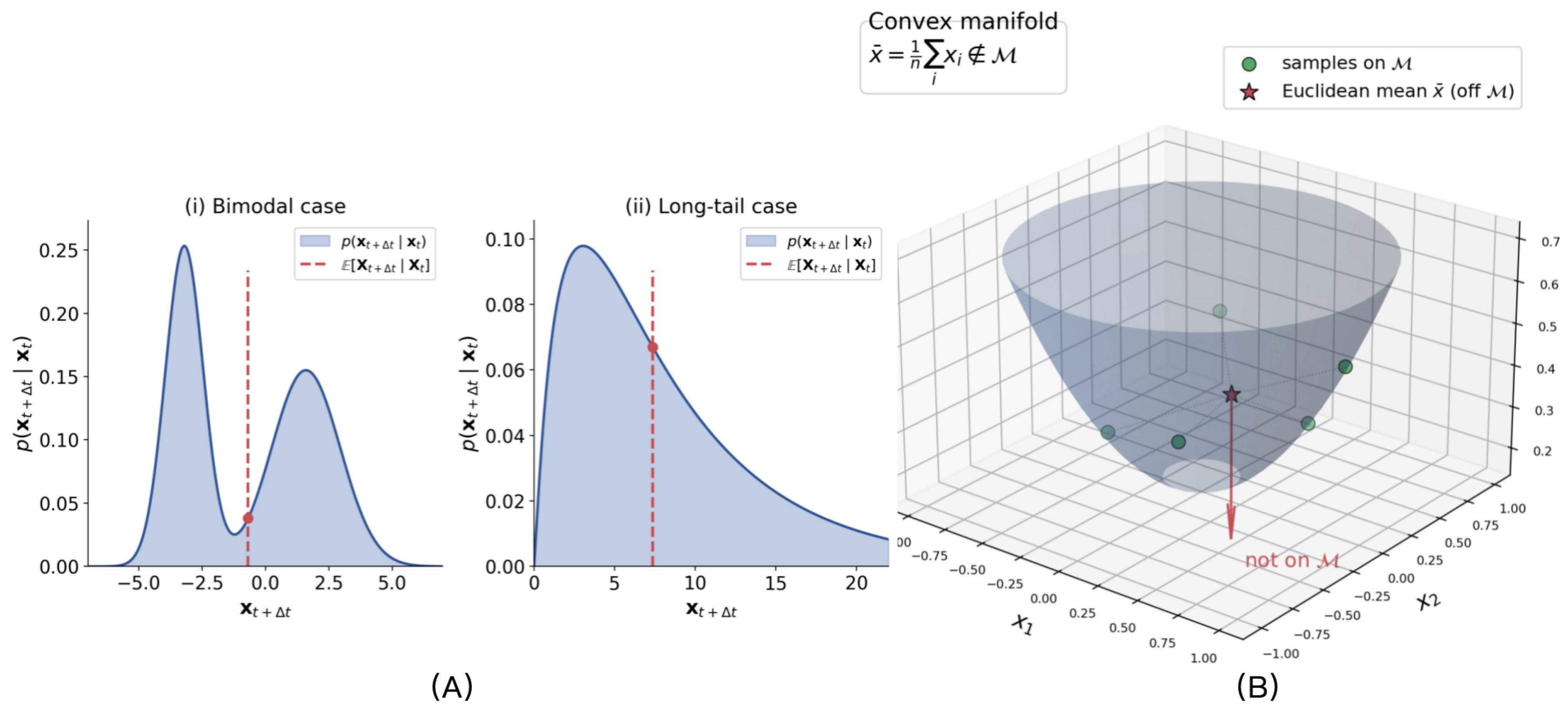
Figure 2.
Markov transition-matrix experiment for (top), (middle), and (bottom). Each row shows, from left to right, the true transition matrix P, the matrix reconstructed from MLP(RMSE) via nearest-state mapping (12), and the matrix learned by MLP(Cross-Entropy). Although RMSE-trained models recover row-wise conditional means with accuracy comparable to the distributional model, they fail to reproduce the full transition law and produce sharply concentrated one-hot rows.
Figure 2.
Markov transition-matrix experiment for (top), (middle), and (bottom). Each row shows, from left to right, the true transition matrix P, the matrix reconstructed from MLP(RMSE) via nearest-state mapping (12), and the matrix learned by MLP(Cross-Entropy). Although RMSE-trained models recover row-wise conditional means with accuracy comparable to the distributional model, they fail to reproduce the full transition law and produce sharply concentrated one-hot rows.
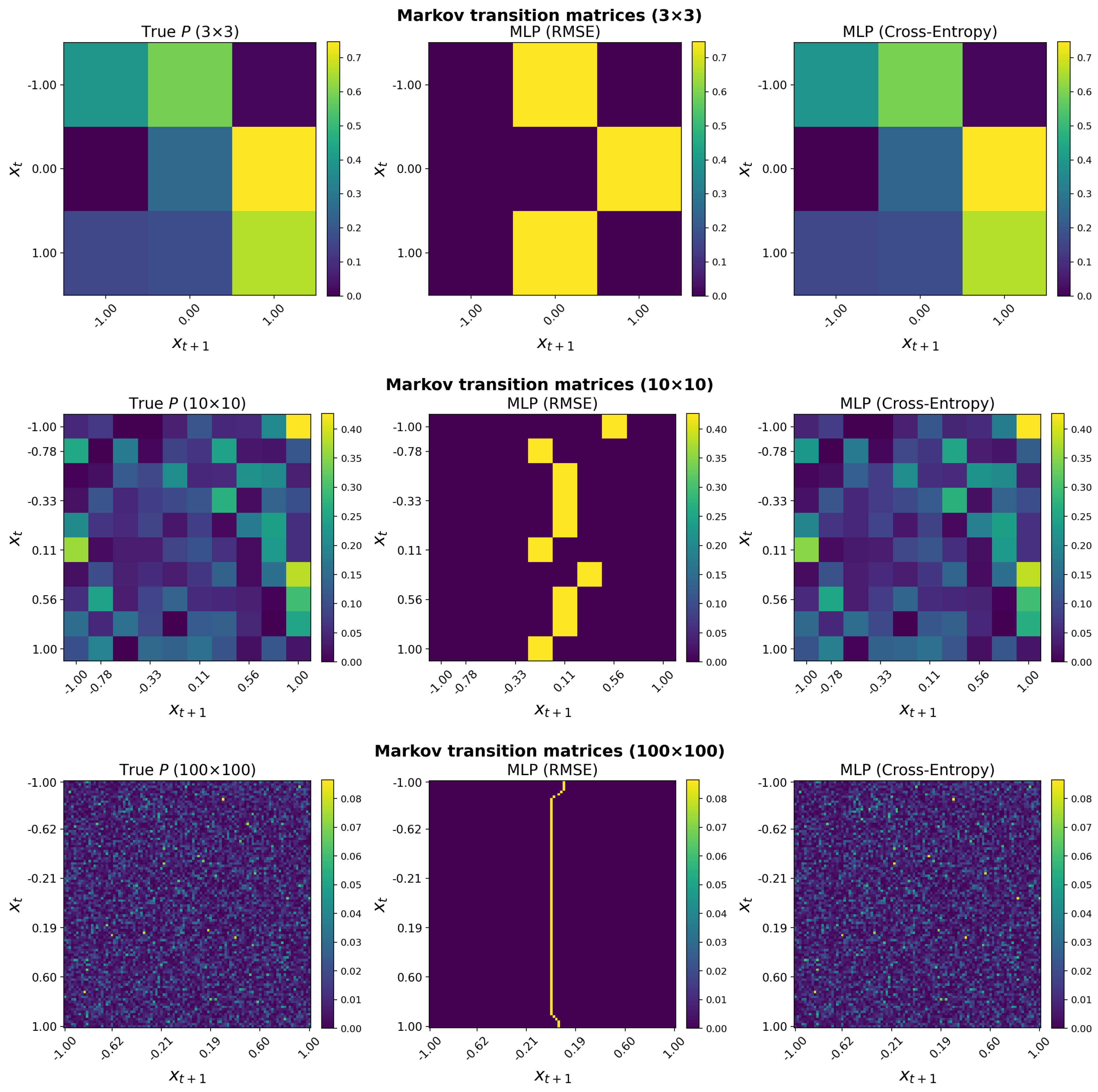
Figure 3.
Rollout of on a random test trajectory. All models share the same initial state. Columns show the truth, the deterministic U-Net, the EDM U-Net ensemble mean (10 members), and two individual EDM samples. At late times, the deterministic forecast and the ensemble mean become smoother, whereas individual diffusion samples retain fine-scale turbulent structure.
Figure 3.
Rollout of on a random test trajectory. All models share the same initial state. Columns show the truth, the deterministic U-Net, the EDM U-Net ensemble mean (10 members), and two individual EDM samples. At late times, the deterministic forecast and the ensemble mean become smoother, whereas individual diffusion samples retain fine-scale turbulent structure.
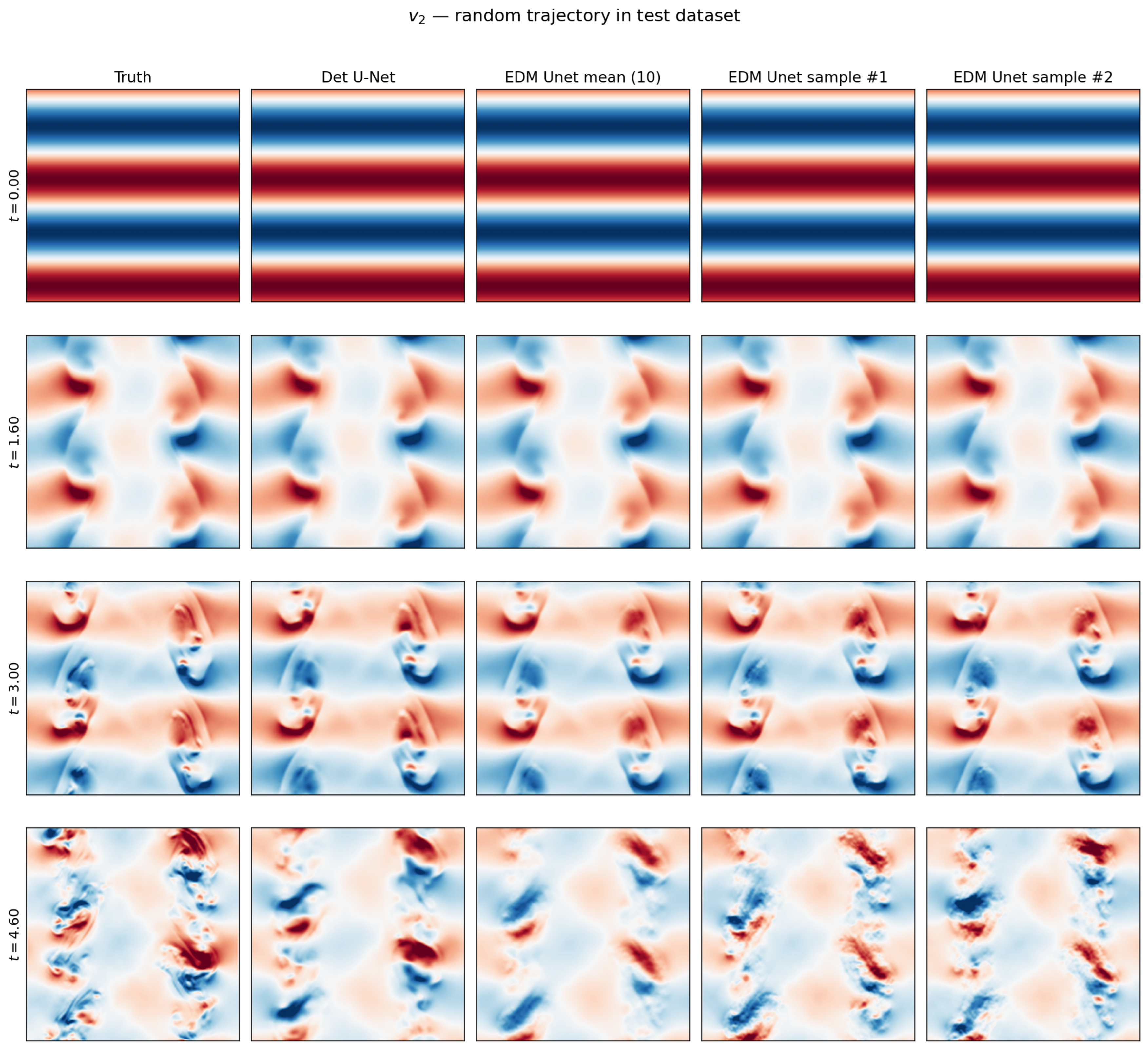
Figure 4.
Radial power spectrum of , averaged over five held-out test members at and . These late times are chosen because the flow is strongly nonlinear and develops pronounced high-frequency structure. Individual EDM samples follow the truth at high wavenumber, while the deterministic U-Net and the diffusion ensemble mean show clear spectral dissipation.
Figure 4.
Radial power spectrum of , averaged over five held-out test members at and . These late times are chosen because the flow is strongly nonlinear and develops pronounced high-frequency structure. Individual EDM samples follow the truth at high wavenumber, while the deterministic U-Net and the diffusion ensemble mean show clear spectral dissipation.
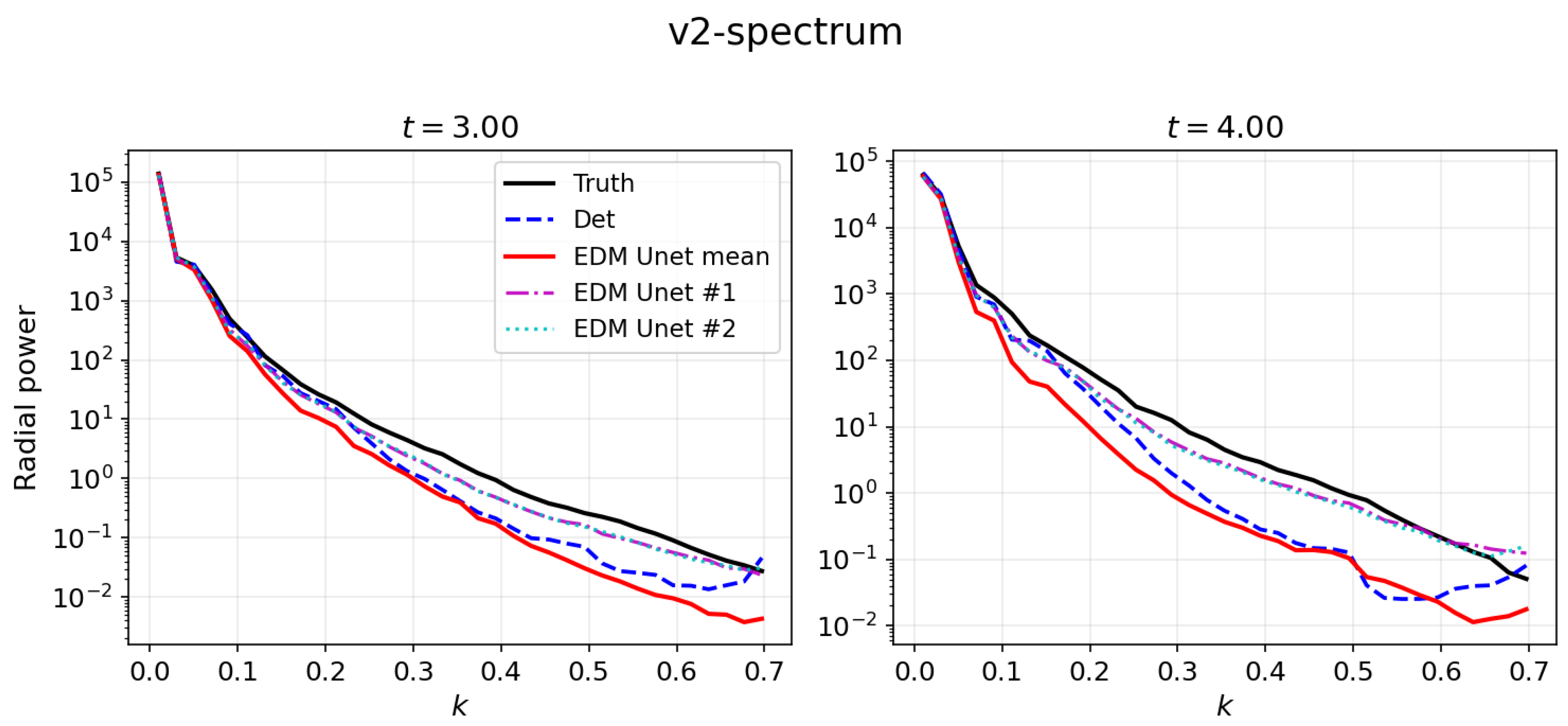

Table 1.
Markov transition-matrix experiment: test RMSE and row-averaged KL divergence for MLP(RMSE) and MLP(Cross-Entropy).
Table 1.
Markov transition-matrix experiment: test RMSE and row-averaged KL divergence for MLP(RMSE) and MLP(Cross-Entropy).
| K | Model | RMSE | KL | Samples / Epochs |
| 3 | MLP(RMSE) | 0.585 | 8.377 | 100,000 / 120 |
| 3 | MLP(Cross-Entropy) | 0.585 | 0.0002 | 100,000 / 120 |
| 10 | MLP(RMSE) | 0.658 | 14.812 | 100,000 / 120 |
| 10 | MLP(Cross-Entropy) | 0.658 | 0.0016 | 100,000 / 120 |
| 100 | MLP(RMSE) | 0.579 | 14.055 | 500,000 / 80 |
| 100 | MLP(Cross-Entropy) | 0.577 | 0.0170 | 500,000 / 80 |
Disclaimer/Publisher’s Note: The statements, opinions and data contained in all publications are solely those of the individual author(s) and contributor(s) and not of MDPI and/or the editor(s). MDPI and/or the editor(s) disclaim responsibility for any injury to people or property resulting from any ideas, methods, instructions or products referred to in the content. |
© 2026 by the authors. Licensee MDPI, Basel, Switzerland. This article is an open access article distributed under the terms and conditions of the Creative Commons Attribution (CC BY) license (http://creativecommons.org/licenses/by/4.0/).
Copyright: This open access article is published under a Creative Commons CC BY 4.0 license, which permit the free download, distribution, and reuse, provided that the author and preprint are cited in any reuse.


