

Submitted:
12 July 2026
Posted:
14 July 2026
You are already at the latest version
Abstract
Ring-core optical fibers support guided electromagnetic fields whose energy can be localized in an annular region rather than near the fiber axis. Such structures are important for higher-order vector modes, annular guided fields, and vortex-compatible optical states. This tutorial presents a step-by-step Maxwell-based derivation of vector modes in a three-layer ring-core optical fiber consisting of an inner cladding, an annular core, and an outer cladding. The purpose is pedagogical rather than to introduce a new eigenmode theory. Starting from Maxwell’s equations in a source-free, lossless, nonmagnetic dielectric medium, we introduce time-harmonic fields, the longitudinal propagation factor exp(iβz), and the azimuthal dependence exp(ilφ). The curl equations are then written explicitly in cylindrical coordinates, yielding six coupled first-order equations for the electromagnetic field components. The system is reduced to the two longitudinal components Ez and Hz, which satisfy Bessel-type radial equations in each homogeneous layer. Regularity at the fiber axis, decay at radial infinity, and continuity of the tangential field components at the two interfaces lead to a homogeneous matrix equation Ml(β)x= 0. The characteristic condition det Ml(β)= 0 determines the allowed propagation constants and effective refractive indices of the guided vector modes. The physical meaning of β, neff, l, radial localization, and annular power confinement is discussed. Particular attention is given to the distinction between annular intensity and vortex phase: an l = 0 mode may be ring-shaped but is not a vortex mode, whereas l ≠ 0 modes possess azimuthal phase winding and are vortex-compatible. Representative numerical illustrations and supplementary code are provided to connect the analytical derivation with modal profiles, intensity maps, phase maps, and power localization in the annular core.
Keywords:
ring-core optical fiber
; vector modes
; Maxwell equations
; cylindrical waveguide
; Bessel functions
; guided modes
; annular core
; azimuthal order
; vortex-compatible modes
; effective refractive index
; boundary-condition matrix
; modal localization
1. Introduction
Ring-core optical fibers form a special class of cylindrical dielectric waveguides in which the optical guiding region is not located at the fiber axis, but occupies an annular domain between an inner and an outer radius. In contrast to a conventional solid-core fiber, where the guided field is usually concentrated near the axis, a ring-core fiber can support modes whose energy is localized mainly in a ring-shaped region.
This geometry is especially relevant for higher-order vector modes, annular guided fields, and vortex-compatible optical states. If a guided field has an azimuthal phase dependence of the form , with integer , then the phase structure is naturally matched to the cylindrical symmetry of the waveguide. For , the field possesses an azimuthal phase winding and can be associated with vortex-like or orbital-angular-momentum-compatible behavior. For , the field is azimuthally phase-uniform and should not be described as a vortex mode, even if its intensity is annular.
The analytical theory of vector modes in three-layer and ring-core optical fibers is well established. Exact eigenvalue equations and field distributions for three-layered radially stratified optical fibers, including ring-core fibers, were formulated by Tsao, Payne, and Gambling [1]. Later, Brunet and co-authors developed vector-mode analysis and cutoff tools for ring-core fibers in the context of spatial-division multiplexing and orbital-angular-momentum mode transmission [2]. Exact cutoff expressions for vector modes in three-layer step-index fibers were also derived in subsequent work [3].
The present paper does not aim to introduce a new eigenmode theory of ring-core fibers. Its purpose is tutorial and methodological. We provide a step-by-step derivation of the guided vector-mode problem starting directly from Maxwell’s equations, with emphasis on the physical meaning of each mathematical step. The presentation is intended for students and researchers in physics, optics, and photonics who need to understand how the characteristic equation for vector modes arises from the electromagnetic boundary-value problem.
1.1. Physical Picture and Tutorial Roadmap
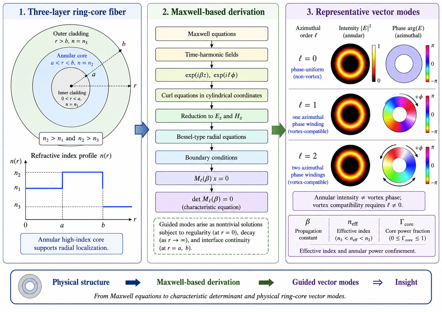
The physical system considered in this tutorial is shown schematically in Figure 1a. The fiber consists of three cylindrical regions: an inner cladding, an annular core, and an outer cladding. The annular core is the guiding region because its refractive index is higher than those of the surrounding regions. In the idealized step-index model, the refractive-index profile is piecewise constant: for , for , and for , with and .
The derivation follows the roadmap shown in Figure 1(b). We begin with Maxwell’s equations in a source-free, lossless, nonmagnetic dielectric medium. The time dependence is then separated by assuming harmonic fields. Since the fiber is uniform along the z-axis, each guided mode is written with a longitudinal propagation factor , where is the propagation constant to be determined.
The cylindrical symmetry of the structure allows the azimuthal dependence to be represented by . The integer character of follows from the requirement that the electromagnetic field must return to the same physical value after a full rotation . Thus, is not an arbitrary fitting parameter; it is the azimuthal order of the mode.
After the longitudinal and azimuthal dependences are introduced, Maxwell’s curl equations are written component by component in cylindrical coordinates. This gives six coupled first-order equations for , and . The central mathematical step is to reduce this system to the longitudinal components and Once these two components are found, the transverse components can be reconstructed from Maxwell’s equations.
In each homogeneous radial layer, and satisfy Bessel-type radial equations. The corresponding layerwise solutions are expressed through Bessel or modified Bessel functions, depending on whether the field is oscillatory or evanescent in the given region. The solutions in the three layers are then connected by the electromagnetic boundary conditions at and . These boundary conditions produce a homogeneous linear system for the unknown expansion coefficients. The existence of a nontrivial guided mode requires the determinant of this system to vanish.
This is the main pedagogical message of the tutorial: guided vector modes are not assumed as predefined field patterns. They arise as nontrivial solutions of Maxwell’s equations subject to symmetry, regularity, decay, and boundary conditions.
1.2. Scope of the Tutorial
The scope of this tutorial is deliberately limited. We consider an ideal three-layer, cylindrically symmetric, lossless, nonmagnetic ring-core optical fiber with a piecewise constant refractive-index profile. The fiber is assumed to be infinite and uniform along the propagation direction. Effects such as bending, ellipticity, random perturbations, material absorption, anisotropy, nonlinear response, and long-distance mode coupling are not included in the basic derivation.
The tutorial also does not attempt to replace the classical theory of optical waveguides. The exact analytical treatment of three-layer optical fibers has already been developed in the literature, and ring-core fibers have been analyzed using vector-mode methods, cutoff theory, and modal design tools. The present paper uses these established results as the scientific background, while focusing on a detailed derivation and physical interpretation.
The emphasis is therefore educational. We show how the characteristic equation for guided vector modes is obtained from Maxwell’s equations step by step. Particular attention is given to the meaning of the modal parameters and , the role of and , the origin of the Bessel-type radial equations, and the way in which boundary conditions lead to the matrix equation .
The numerical examples included at the end of the paper are used only to illustrate the analytical construction. They show representative effective indices, radial profiles, intensity maps, and phase maps for selected azimuthal orders. They are not intended as a complete design study of ring-core fibers. More advanced problems, such as multi-ring-core optimization, inter-ring modal control, and energy-optimal superpositions of vector modes, are outside the scope of this tutorial and are reserved for subsequent work.
Thus, the present work should be understood as a Maxwell-based tutorial reconstruction of the known vector-mode formulation, not as a new analytical theory of ring-core fiber eigenmodes.
2. Known Analytical Background
The electromagnetic description of optical fiber modes is based on Maxwell’s equations. In a source-free dielectric medium, these equations determine how the electric and magnetic fields are coupled through the material permittivity and permeability. In optical waveguide theory, the modal problem is obtained by looking for nontrivial field distributions that satisfy Maxwell’s equations together with regularity, decay, and boundary conditions at material interfaces.
The general electromagnetic and optical-waveguide theory used in this tutorial is presented in several classical and educational texts. Snyder and Love provide a rigorous treatment of guided modes, propagation constants, hybrid modes, and electromagnetic boundary conditions in dielectric waveguides [4]. Complementary derivations and physical interpretations of optical-waveguide and fiber modes can be found in the textbooks by Okamoto [5], Marcuse [6], Bures [7], and Saleh and Teich [8]. In the present tutorial, we follow this established Maxwell-based framework but reconstruct the derivation explicitly for the three-layer ring-core geometry. The analytical treatment of three-layer optical fiber waveguides was developed in detail by Tsao, Payne, and Gambling. They formulated exact eigenvalue equations and corresponding field distributions for general three-layered, radially stratified optical fibers using Debye potentials and Bessel-function combinations. Their method was applied to several practical structures, including fibers with a central index depression, W fibers, progressively stepped three-layer structures, and ring-core fibers [1].
Ring-core fibers were later analyzed in the context of spatial-division multiplexing and orbital-angular-momentum transmission. Brunet et al. considered an annular, or ring-core, step-index fiber and developed analytical expressions for the eigenmodes and modal cutoff conditions. They emphasized that vector eigenmode maps are more appropriate than scalar weak-guidance LP-mode maps when one wants to predict or target modes relevant to orbital angular momentum transmission [2].
The same research line was extended to three-layer step-index fibers by Brunet, Bélanger, and Rusch. They derived exact cutoff expressions for vector and scalar modes in all three-layer step-index fiber geometries and pointed out that such cutoff expressions are useful for predicting the number of supported modes for a given fiber profile. They also explicitly note that vector modes for such fibers had already been solved, while their contribution concerned exact cutoff expressions [3].
Beyond the derivation of cutoff conditions, ring-core fibers have been investigated as natural guiding structures for optical fields with annular intensity and azimuthal phase winding. The relation between optical vortices and guided fiber modes was reviewed by Ramachandran, Kristensen, and Yan [9]. Subsequent studies addressed the design and fabrication of families of ring-core fibers for orbital-angular-momentum transmission [10], summarized the main principles and limitations of OAM-guiding fibers [11], and experimentally demonstrated high-capacity OAM mode-division multiplexing in a specially designed fiber [12].
These works establish an important point for the present paper: the existence of guided vector modes in three-layer and ring-core optical fibers is not a new result. Characteristic equations, cutoff conditions, and vector-mode descriptions are already available in the literature. Therefore, the contribution of this tutorial is not the discovery of ring-core vector modes, but the step-by-step reconstruction of the derivation in a form suitable for teaching and self-study.
The approach taken here differs from the compact formalism used in many advanced treatments. Instead of starting from Debye potentials or presenting only final characteristic equations, we begin with Maxwell’s curl equations and explicitly introduce the harmonic time dependence, the longitudinal factor , and the azimuthal factor . We then write the cylindrical curl equations component by component and show how the transverse field components can be expressed through the longitudinal components and .
This choice of presentation is intentional. For many readers, the most difficult part of the theory is not the final determinant equation itself, but the chain of reasoning that connects Maxwell’s equations with the Bessel-function representation of the fields and the boundary-condition matrix. The tutorial therefore focuses on the intermediate steps: the meaning of , the integer nature of , the difference between and modes, the origin of the radial Bessel equations, and the construction of the homogeneous system .
In summary, the present work should be read as a pedagogical bridge between the classical electromagnetic theory of guided modes and the modern use of ring-core fibers for annular and vortex-compatible optical fields. It uses established analytical results as its foundation, while making the derivation transparent for students and researchers who need to understand how the vector eigenmode problem is built from Maxwell’s equations.
In addition to the eigenmode and cutoff problems considered in [1,2,3], the practical excitation of ring-core modes requires spatial, phase, polarization, and radial matching between the incident field and the guided vector mode. Metasurface-assisted coupling and the associated metrological tolerances have been considered in [13].
3. Geometry and Assumptions
The aim of this section is to define the physical waveguide model used throughout the tutorial. We consider the simplest ring-core configuration that still contains the essential physics of annular guiding: a three-layer cylindrical optical fiber consisting of an inner cladding, an annular core, and an outer cladding.
3.1. Three-Layer Ring-Core Geometry
We use cylindrical coordinates , where is the fiber axis, is the radial distance from the axis, and is the azimuthal angle. The fiber is assumed to be infinitely extended and uniform along the -direction. Therefore, the refractive-index profile depends only on the radial coordinate .
The three radial regions are defined as follows. Region 1 is the inner cladding, , with refractive index . Region 2 is the annular core, , with refractive index . Region 3 is the outer cladding, , with refractive index .
The corresponding refractive-index profile and guiding-index condition are
with
The annular layer is therefore the guiding region. This condition means that the ring core has a higher refractive index than both surrounding regions. Physically, this is the reason why a guided field may be concentrated in the annular region rather than in the central part of the fiber or in the outer cladding.
The radii a and b are the inner and outer radii of the ring core, respectively. The ring thickness is . The idealized outer cladding is treated as radially unbounded. In a real fiber, the outer cladding has a finite radius, but the unbounded-cladding approximation is standard when the modal field decays sufficiently before reaching the physical outer boundary.
3.2. Material Assumptions
The medium is assumed to be linear, isotropic, nonmagnetic, and lossless. Under these assumptions, the magnetic permeability is equal to the vacuum permeability, the electric permittivity is determined by the refractive-index profile, and no free electric charges or free electric currents are present in the fiber:
Here is the vacuum permeability, is the vacuum permittivity, and is the piecewise constant refractive-index profile defined in Eq. (1).
Because the refractive indices , , and are assumed real, the model does not include material absorption. Losses due to bending, microbending, surface roughness, fabrication imperfections, or radiation leakage are also excluded from the basic derivation.
These assumptions are deliberately idealized. Their purpose is to obtain the clean electromagnetic eigenvalue problem from Maxwell’s equations. More complicated effects can be added later as perturbations or as separate physical mechanisms, but they are not needed for the tutorial derivation.
3.3. Modal Assumptions
We seek guided electromagnetic modes that propagate along the z-axis without changing their transverse field structure. Such a mode has a longitudinal phase factor determined by a propagation constant . The value of is not imposed in advance; it is found as an eigenvalue of the boundary-value problem.
For a guided mode localized mainly in the annular core, the propagation constant is expected to lie between the cladding and core wavenumbers. Anticipating the harmonic formulation used below, we introduce the free-space wavenumber and the effective refractive index as
The first inequality gives the guided-mode interval in terms of the propagation constant . The second gives the same condition in terms of the effective refractive index . The upper bound allows the field in the annular core to have an oscillatory radial character, whereas the lower bound ensures evanescent behavior in both lower-index surrounding regions. Therefore, the mode can remain radially confined.
This form is often more intuitive: the effective refractive index of the guided mode must be smaller than the refractive index of the guiding ring, but larger than the refractive indices of the surrounding claddings.
3.4. Regularity and Decay Conditions
The electromagnetic field must be physically acceptable in all three regions.
First, the field must remain finite at the fiber axis . This requirement excludes singular radial functions in the inner region. In particular, Bessel-type functions that diverge at cannot be used in Region 1.
Second, the field must decay as in the outer cladding. This requirement excludes radially growing solutions in Region 3. Only decaying radial functions are allowed in the outer region.
Third, at the material interfaces and , the tangential components of the electromagnetic fields must be continuous. These boundary conditions will later provide the algebraic equations for the unknown expansion coefficients.
Thus, the complete guided-mode problem consists of four ingredients: Maxwell’s equations in each homogeneous layer, regularity at , decay as , and continuity of tangential field components at and . These conditions convert the electromagnetic problem into an eigenvalue problem for .
3.5. Comment on the Role of the Annular Core
It is important not to confuse two different ideas. The annular core determines where the field can be radially localized, but it does not by itself determine whether the mode is vortex-like. Radial localization is controlled by the refractive-index profile , while vortex-compatible behavior is associated with the azimuthal phase factor .
Therefore, an = 0 mode may still be concentrated in the ring core, but it is azimuthally phase-uniform and does not have a nonzero topological charge. Modes with ≠ 0 have an azimuthal phase winding and are the relevant candidates for vortex-compatible guided states.
This distinction will be important in the following sections. The same ring-core geometry can support both phase-uniform annular modes and vortex-compatible modes. The difference between them is not the radial shape alone, but the azimuthal phase structure.
4. Maxwell Equations in a Lossless Nonmagnetic Medium
The guided modes of the ring-core fiber are electromagnetic fields. Therefore, the starting point of the derivation is not a scalar wave equation, but the full Maxwell system. In this section, we write Maxwell’s equations for the material model introduced in Section 3.
Consistently with the material assumptions stated in Eq. (2), the fiber is treated as a source-free dielectric medium. Thus, there are no free electric charges and no free electric currents inside the fiber. The time-domain Maxwell equations are therefore written as
Here is the electric field, is the magnetic field, is the electric displacement field, and is the magnetic flux density.
For a linear, isotropic, nonmagnetic dielectric, the constitutive relations are
Substituting Eq. (5) into the curl equations in Eq. (4), and using the fact that is time independent, we obtain the time-domain curl equations used in the modal derivation:
These two equations are the dynamical part of Maxwell’s system. They describe how a time-varying magnetic field generates a rotational electric field and how a time-varying electric displacement generates a rotational magnetic field.
The divergence equations remain
In each homogeneous layer of the fiber, is constant. Therefore, inside a single layer the first divergence equation reduces to . At the interfaces and , however, changes discontinuously. For this reason, the divergence equation must be understood together with the electromagnetic boundary conditions at the material interfaces.
For the derivation of the guided modes, the curl equations in Eq. (6) are the main working equations. The divergence equations are not discarded; rather, they are automatically respected when the full Maxwell system and the correct boundary conditions are satisfied. The boundary conditions will be introduced later, after the field components have been expressed in cylindrical coordinates.
The next step is to pass from the time-domain equations to harmonic fields. This will convert the time derivatives in Eq. (6) into multiplication by and will produce the frequency-domain Maxwell equations used for the modal analysis.
5. Time-Harmonic Representation
The fields in a guided optical mode oscillate in time at an optical angular frequency ω. Instead of working directly with real time-dependent sinusoidal fields, it is convenient to use complex field amplitudes. The physical fields are then understood as the real parts of complex expressions.
In this tutorial, we use the time convention
Here and are complex spatial amplitudes. The physical electric and magnetic fields are obtained by taking the real parts of the corresponding complex expressions:
The use of complex amplitudes does not change the physical problem. It is a mathematical representation of sinusoidal time dependence. The real measurable fields are obtained by taking the real part at the end.
Because the time dependence is differentiation with respect to time gives
and similarly for the magnetic field. Thus, for harmonic fields with the convention the time derivative is replaced by multiplication by :
Applying Eq. (8) to the time-domain curl equations in Eq. (6) gives the frequency-domain Maxwell curl equations
These equations are written for the complex spatial amplitudes and . From this point onward, the symbols and denote these complex amplitudes unless stated otherwise.
Using the free-space wavenumber introduced in Eq. (3), the material wavenumber in a homogeneous layer with refractive index is
This notation will be used later when deriving the radial Bessel-type equations in each layer.
The sign convention in Eq. (7) should be kept consistent throughout the derivation. If one instead uses , the signs in the frequency-domain curl equations are reversed. Some optical-fiber texts use the equivalent convention . The physical field is unchanged if one convention is used consistently; however, the signs in the frequency-domain curl equations and in the transverse-field reconstruction formulas must not be mixed.
The next step is to use the translational symmetry of the fiber along the -axis. This will allow us to introduce the longitudinal propagation factor , where is the propagation constant of the guided mode.
6. Longitudinal Propagation Factor
The ring-core fiber considered in this tutorial is assumed to be uniform along the -axis. Its refractive-index profile depends only on the radial coordinate r and does not depend on . Therefore, the transverse structure of an ideal guided mode does not change as the mode propagates along the fiber. The field may acquire phase along , but its transverse profile remains the same.
This physical property motivates the longitudinal modal representation
Here is the longitudinal propagation constant. With the time convention introduced in Eq. (7), the full time-dependent fields contain the total phase factor . For , a surface of constant phase moves in the positive -direction. Therefore, with the convention , positive corresponds to forward propagation along .
The propagation constant is not chosen freely. It must be determined from the electromagnetic boundary-value problem. Only special values of allow the fields to satisfy Maxwell’s equations, regularity at , decay as , and boundary conditions at and . For this reason, is an eigenvalue of the guided-mode problem.
Because every field component contains the same longitudinal factor , differentiation with respect to becomes multiplication by . This derivative rule will be combined with the azimuthal derivative rule in Section 7.
The effective refractive index was already defined in Eq. (3) as . Thus, and neff describe the same modal propagation property in two equivalent forms: gives the longitudinal phase accumulation per unit length, while expresses this propagation constant in refractive-index units.
For a guided mode localized in the ring core, the expected interval is the one stated in Eq. (3):
or equivalently,
The upper inequality allows the field in the annular core to have an oscillatory radial dependence. The lower inequality makes the field evanescent in the lower-index surrounding regions. This is the mathematical expression of transverse confinement in a step-index ring-core fiber.
The next symmetry to use is the cylindrical symmetry of the waveguide. Since the refractive-index profile does not depend on the azimuthal coordinate , the angular dependence of each mode can be represented by the factor .
7. Azimuthal Dependence
The ring-core fiber is cylindrically symmetric. Its refractive-index profile depends only on the radial coordinate and does not depend on the azimuthal coordinate φ. This means that the physical structure remains unchanged after a rotation around the fiber axis. Therefore, the angular part of a guided mode can be chosen as an eigenfunction of rotations around the -axis.
For any electromagnetic field component , where denotes one of , or , the separated modal form is written as
Here is the radial amplitude, is the propagation constant, and is the azimuthal order. This compact notation replaces the separate listing of the six component expressions. The same angular and longitudinal factors are used for all field components, while the radial amplitudes remain component-dependent functions of .
The integer character of follows from the single-valuedness of the electromagnetic field. After one complete rotation around the fiber axis, the physical point is the same: . Therefore, each field component must return to the same value. For the azimuthal factor this gives
Thus, must be an integer:
= 0, ±1, ±2, ±3, ...
This integer is the azimuthal order of the guided mode. It describes how many phase cycles are accumulated when moving once around the fiber axis.
For , the azimuthal factor is . In this case, the field has no azimuthal phase winding. Its phase does not change when increases from 0 to . Such a mode may still have an annular intensity distribution because the refractive-index profile is ring-shaped, but it is not a vortex mode in the scalar phase sense. It is better to describe it as an azimuthally phase-uniform annular mode.
For , the phase changes continuously with . After one full rotation, the accumulated phase is . Thus, a mode with = 1 accumulates a phase change of , a mode with = 2 accumulates , and so on. The sign of determines the handedness of the azimuthal phase winding. Positive and negative values of correspond to opposite helical phase directions.
This is the reason why modes with are called vortex-compatible in this tutorial. The term “vortex-compatible” is used deliberately. In a full vector fiber mode, the field may contain nontrivial polarization structure and may correspond to hybrid or modes rather than to an ideal scalar orbital-angular-momentum state. Therefore, the azimuthal factor is a necessary indicator of vortex-like phase structure, but the complete physical mode must still be treated as a vector electromagnetic field.
With the longitudinal and azimuthal factors introduced, the differential operations reduce to
The radial derivative is not replaced by a constant, because the radial amplitudes remain unknown functions of . These substitutions are the key preparation for the next section. We can now write the curl equations in cylindrical coordinates and transform Maxwell’s equations into six coupled ordinary differential equations for the radial field amplitudes.
8. Curl Equations in Cylindrical Coordinates
The ring-core fiber has cylindrical symmetry. Therefore, Maxwell’s equations must be written in cylindrical coordinates rather than in Cartesian coordinates. In this section, we write the curl operator explicitly for a general vector field and then apply it to the electric and magnetic fields.
Let A be a vector field expressed in cylindrical coordinates as where , , and are the unit vectors in the radial, azimuthal, and axial directions, respectively.
In cylindrical coordinates, the curl of is
This formula is one of the key technical steps in the derivation. It differs from the Cartesian curl because the cylindrical basis vectors depend on the angular coordinate , and because the azimuthal coordinate has the scale factor . This is the reason why terms such as 1/r and appear.
Applying Eq. (15) to the electric field gives
Similarly, applying Eq. (15) to the magnetic field gives
The frequency-domain Maxwell curl equations obtained in Section 5 are given in Eq. (9):
The cylindrical curl expressions now allow us to compare the radial, azimuthal, and axial components of both sides of these equations. This comparison produces six scalar equations: three from and three from .
Using the modal derivative rules in Eq. (14), the partial differential equations in , and are converted into ordinary differential equations in the radial variable . The reason is that the dependence on and has already been separated through the factors and , while the radial amplitudes remain unknown functions of .
Thus, after the cylindrical curl expressions are written, the next step is straightforward but important: substitute the curl components into the frequency-domain Maxwell equations and use Eq. (14). This gives the six first-order radial equations for , and . These equations form the starting point for reducing the vector problem to the two longitudinal components and .
9. Six First-Order Equations for ,
We now substitute the cylindrical curl expression in Eq. (15) into the frequency-domain Maxwell equations in Eq. (9). This gives six coupled first-order equations for the radial amplitudes of the electromagnetic field components.
Inside each homogeneous layer, the refractive index is constant. Therefore, in layer j we write where . The equations below are written inside one homogeneous layer, so is constant within that layer.
All field components are assumed to have the separated modal dependence introduced in Eq. (12). Therefore, the derivative substitutions in Eq. (14) apply:
Comparing the radial, azimuthal, and axial components of both sides of the two curl equations gives the complete six-component first-order system:
The first three equations in Eq. (16) come from . The last three equations come from
This system is still a full vector system: all six field components are present. However, it contains the key structure that makes the reduction possible. The transverse components , and can be expressed algebraically through the longitudinal components and and their radial derivatives. After that, the remaining equations lead to second-order radial equations for and .
It is important to emphasize that Eq. (16) is valid separately in each homogeneous layer. The material parameter changes from one layer to another:
Therefore, the radial dependence of the fields is solved independently in each layer and then connected at the interfaces and by boundary conditions. These boundary conditions are not imposed yet; they will be introduced after the layerwise radial solutions have been obtained.
The next step is to solve part of Eq. (16) for the transverse field components , and in terms of , and . This reduction is the central algebraic step that converts the full six-component Maxwell system into a pair of Bessel-type radial equations for the longitudinal components.
10. Reduction to Ez and Hz
The six first-order equations obtained in Section 9 contain all components of the electromagnetic field. However, the six components do not need to be solved independently. A standard and very useful feature of cylindrical waveguide theory is that the transverse field components can be expressed through the two longitudinal components and .
The derivation is performed inside one homogeneous layer . We use
Here is the material wavenumber in layer , and is the transverse spectral parameter. The sign of depends on the layer. In the guiding annular core, may be positive, corresponding to oscillatory radial behavior. In a lower-index cladding for a guided mode, is typically negative, corresponding to evanescent radial behavior.
The algebraic reduction below is valid when ≠ 0. The special case = 0 corresponds to a cutoff or transition case and must be treated by an appropriate limiting procedure.
We use the four equations in Eq. (16) that contain the transverse components algebraically:
Solving this algebraic subsystem for , , , and gives
These four relations are the central result of the reduction. They show that once and ) are known in a given layer, all transverse field components can be reconstructed directly.
The physical meaning of this result is important. In a vector fiber mode, the transverse and longitudinal components are not independent. Maxwell’s curl equations couple them. The longitudinal fields and determine the transverse circulation of the electromagnetic field, while the transverse components are required to satisfy the full vector character of Maxwell’s equations.
For = 0, the terms proportional to vanish. In that case, Eq. (18) reduces to
This special case shows clearly that an = 0 mode can still have nonzero radial and azimuthal field components, but it does not have azimuthal phase winding. Therefore, = 0 remains a non-vortex azimuthally phase-uniform mode.
For ≠ 0, the terms proportional to couple with and , and with Er and . This coupling is one of the reasons why higher-order modes in fibers must generally be treated as vector modes rather than as purely scalar fields.
Substitution of Eq. (18) into the remaining Maxwell equations leads to second-order equations for and . Equivalently, and more transparently for the present tutorial, the same equations can be obtained from the vector Helmholtz equations derived directly from Maxwell’s curl equations, as shown in the next section.
11. Bessel-Type Radial Equations
In the previous section, the transverse field components were expressed through the longitudinal components and . Therefore, the remaining task is to find the radial dependence of and in each homogeneous layer of the fiber.
Inside each homogeneous layer , the refractive index , the permittivity , and the permeability are constant, while the material wavenumber and the transverse spectral parameter are defined in Eq. (17). Taking the curl of the first frequency-domain Maxwell equation and using the second one gives
Using the vector identity
and the fact that inside a homogeneous source-free layer, we obtain
The same procedure gives
Taking the longitudinal component of either vector equation gives
where . Substituting the modal dependences and then gives Eq. (19).
After substituting the separated modal dependence introduced in Eq. (12), both longitudinal components satisfy the same radial equation:
Equation (19) is the Bessel-type radial equation for the longitudinal field components in layer j. The term determines whether the radial dependence is oscillatory or evanescent in the given layer. The term arises from the azimuthal dependence , and therefore the azimuthal order, directly affects the radial structure of the mode.
When > 0, Eq. (19) has oscillatory Bessel-function solutions. This is the usual situation in the guiding annular core for a bound mode.
When < 0, it is convenient to write
Then Eq. (19) becomes
This is the modified Bessel equation. Its solutions are modified Bessel functions, which describe radially increasing or decreasing behavior. For a guided mode in the outer cladding, only the decreasing solution is physically acceptable as
For a guided mode of the three-layer ring-core fiber, the usual situation is
Here and are the radial decay parameters in the inner and outer claddings, respectively, while u is the oscillatory radial parameter in the annular core.
Thus, the field is oscillatory in the high-index annular core and evanescent in the surrounding lower-index regions. This is the mathematical expression of radial confinement.
It is important to emphasize that Eq. (19) does not yet determine the allowed values of . For any trial value of , one can formally write radial solutions in each layer. However, only special values of allow these solutions to satisfy regularity at , decay as , and continuity of the tangential field components at and . These allowed values of will be obtained later from the characteristic condition.
The next step is to write the explicit layerwise solutions of Eq. (19) in the inner cladding, annular core, and outer cladding.
12. Layerwise Solutions
The radial equations obtained in Section 11 must be solved separately in each homogeneous layer of the fiber. Since the refractive index is piecewise constant, the functional form of the solution depends on the sign of the transverse spectral parameter in each layer.
For the guided-mode interval stated in Eq. (3), the field is evanescent in the inner and outer claddings and oscillatory in the annular core. Therefore, the solutions are written using modified Bessel functions in the claddings and ordinary Bessel functions in the core.
12.1. Inner Cladding: 0 < r < a
In the inner cladding, < 0, and the radial equation has the modified Bessel form. The two independent solutions are and . However, the physical field must remain finite at the fiber axis .
The function ) is finite at , while is singular at . Therefore, the solution is excluded in the inner cladding.
12.2. Annular Core: a < r < b
In the annular core, = u² > 0. The radial equation is the ordinary Bessel equation. Its two independent solutions are and .
In a conventional solid-core fiber, the solution is usually excluded because it is singular at . In the present ring-core geometry, however, the annular core occupies only the interval and does not include the axis . Therefore, both and are admissible in the annular core.
12.3. Outer Cladding: r > b
In the outer cladding, < 0, and the radial equation again has the modified Bessel form. The two independent solutions are and . Their behavior at large r is different: grows exponentially, while decays exponentially.
For a guided mode, the field must not grow without bound in the outer cladding. Therefore, the solution is excluded, and only the decaying solution is retained.
12.4. Complete Layerwise Representation
Combining the three regions, the longitudinal electric field is represented as
Similarly, the longitudinal magnetic field is represented as
The unknown coefficient vector is
The order of coefficients in Eq. (24) is not unique, but it must be kept fixed when constructing the boundary-condition matrix. In this tutorial, the ordering in Eq. (24) will be used.
Once and are known in each layer, the transverse field components and are obtained from the reconstruction formulas in Eq. (18). Therefore, the layerwise expressions in Eqs. (22) and (23) are sufficient to reconstruct the complete vector electromagnetic field.
12.5. Derivatives Needed for Transverse Fields
The transverse-field reconstruction formulas in Eq. (18) contain the radial derivatives of and . Therefore, after the longitudinal fields are written in the form of Eqs. (22) and (23), their derivatives must also be evaluated in each layer.
In the inner cladding, , we have
In the annular core, , the derivatives are
In the outer cladding, , they are
Here the prime denotes differentiation with respect to the full argument of the Bessel function. For example,
evaluated at
The additional factors , u, and appear because the derivative is taken with respect to , while the Bessel functions depend on the products , ur, and . This is simply the chain rule.
These derivative expressions will be used when the tangential components and are evaluated at the interfaces and . In particular, the continuity of involves , while the continuity of involves , as follows directly from Eq. (18).
12.6. Physical Interpretation of the Layerwise Solutions
The layerwise solutions encode three physical requirements of a guided ring-core mode. In the high-index annular core, , so the longitudinal fields have oscillatory Bessel-function dependence. Because the annular region does not include the axis , both and are admissible.
In the inner cladding, regularity at the fiber axis excludes the singular function and retains . In the outer cladding, decay at radial infinity excludes the growing function and retains .
Thus, Eqs. (22) and (23) represent an oscillatory field in the annular guiding region and evanescent fields in the surrounding claddings. The remaining coefficients are determined by the electromagnetic boundary conditions at and .
13. Boundary Conditions
The layerwise solutions obtained in Section 12 are valid separately in the inner cladding, annular core, and outer cladding. To form a physical guided mode of the complete fiber, these solutions must be connected at the material interfaces. The connection is provided by the electromagnetic boundary conditions.
The two interfaces of the three-layer ring-core fiber are and . The interface separates the inner cladding from the annular core. The interface separates the annular core from the outer cladding.
Since there are no free surface charges and no free surface currents at these dielectric interfaces, the tangential components of the electric and magnetic fields must be continuous. At a cylindrical interface = constant, the normal direction is radial. Therefore, the tangential directions are the azimuthal direction and the axial direction .
Thus, the tangential field components are , and .
At the two interfaces, the boundary conditions are
at r = a:
at r = b:
These eight scalar equations connect the eight unknown expansion coefficients introduced in Eq. (24):
The continuity of and can be written directly using the longitudinal layerwise solutions in Eqs. (22) and (23). For example, at the direct continuity conditions give
At , they give
The continuity of and is obtained by using the transverse-field reconstruction formulas in Eq. (18). This is an important point: the boundary conditions are imposed on the tangential field components, but and are not independent unknown functions. They are reconstructed from , and .
For example, at , the condition means that where each is computed from Eq. (18) using the parameters and Bessel-function solutions appropriate to layer . Similarly, the condition is evaluated using the expression for in Eq. (18).
The same procedure is applied at . Thus, all eight boundary conditions in Eq. (25) become linear algebraic equations for the eight coefficients , and It is useful to emphasize the physical meaning of these boundary conditions. The field may change its radial functional form when passing from one layer to another because the refractive index changes. However, the tangential electromagnetic field itself cannot jump across an ideal dielectric interface without free surface current or singular surface sources. Therefore, the Bessel-function amplitudes in the three layers are not independent; they must be matched at the interfaces.
The normal components also obey electromagnetic boundary conditions: the normal component of and the normal component of are continuous in the absence of free surface charge and magnetic monopoles. In the present formulation, once the fields satisfy Maxwell’s equations in each layer and the tangential continuity conditions are imposed consistently, the remaining normal conditions are not independent additional equations for the modal determinant. The characteristic equation is therefore constructed from the continuity of , and The next step is to arrange the eight boundary equations into a matrix form. This gives the homogeneous linear system
14. Matrix Equation
The eight boundary conditions in Eq. (25) form a homogeneous system of linear equations for the eight unknown expansion coefficients. Using the coefficient vector defined in Eq. (24), this system can be written compactly as
14.1. Explicit Construction of the Boundary-Condition Matrix
To make the derivation fully reproducible, the entries of the boundary-condition matrix are written explicitly below. We retain the coefficient ordering introduced in Eq. (24):
The ordering of these coefficients must remain fixed because every column of the boundary-condition matrix corresponds to one particular coefficient in this vector.
For compact notation, we introduce the values of the Bessel and modified Bessel functions at the two interfaces. At the inner interface , let
and
At the outer interface , let
and
Here the prime denotes differentiation with respect to the complete argument of the corresponding Bessel function. For example, denotes evaluated at .
The transverse parameters satisfy
and the permittivity in layer is .
Let denote the -th row of . With the coefficient ordering given above, the eight rows are obtained as follows.
Row 1: continuity of at
The condition
gives
Row 2: continuity of at
The condition
gives
Row 3: continuity ofat
Using the reconstruction relation
the condition
gives
Row 4: continuity ofat
Using
the condition
gives
Row 5: continuity of at
The condition
gives
Row 6: continuity of at
The condition
gives
Row 7: continuity ofat
The condition
gives
Row 8: continuity of at
The condition
gives
The complete boundary-condition matrix is therefore formed by arranging these row vectors in the same order:
Each row corresponds to one electromagnetic boundary condition, while each column corresponds, respectively, to the coefficients
Thus, the matrix explicitly connects the longitudinal electric- and magnetic-field amplitudes in the inner cladding, annular core, and outer cladding.
The system in Eq. (26) is homogeneous because no external source or prescribed incident field is imposed. We are looking for self-sustained guided modes of the fiber. Therefore, the zero vector is always a mathematical solution, but it corresponds to the absence of an electromagnetic field and is physically irrelevant.
A physical guided mode requires a nonzero coefficient vector. Such a nontrivial solution can exist only if the explicitly constructed matrix is singular.
This singularity condition leads to the characteristic equation considered in the next section.
15. Characteristic Condition det
The homogeneous system in Eq. (26) has a nontrivial solution only when its coefficient matrix is singular. Therefore, the condition for the existence of a guided mode is
This equation is the characteristic equation of the three-layer ring-core fiber for the azimuthal order, . It determines the allowed values of the propagation constant β.
It is useful to introduce the characteristic function
The roots of this equation are the modal propagation constants. Each root may be denoted as , where is the azimuthal order and m labels different radial branches for the same .
Once a root is found, the corresponding effective refractive index is
For a bound mode localized mainly in the annular core, this effective index must lie in the guided-mode interval stated in Eq. (3):
Equivalently,
This interval has a direct physical interpretation. If is smaller than the cladding wavenumber, the field is not radially confined. If is larger than the core wavenumber, the field cannot have the required oscillatory behavior in the guiding annulus. Therefore, guided ring-core modes are searched for within this interval.
The determinant equation does not directly give the field amplitude. It gives the allowed propagation constants. After a root has been found, the matrix becomes singular, and the coefficient vector is obtained from
This vector spans the null space of . Because the system is homogeneous, the absolute scale of is arbitrary. Multiplying all coefficients by the same nonzero constant produces the same modal profile with a different amplitude. Therefore, an additional normalization condition is needed if one wants to assign a definite power to the mode.
For example, one may normalize the mode by fixing the longitudinal power flow,
where is the -component of the time-averaged Poynting vector and is the transverse area element.
Such normalization is not needed for deriving the characteristic equation, but it is important for coupling calculations, modal overlaps, and comparisons of modal energy localization.
The determinant condition also clarifies the role of the boundary conditions. For a general trial value of , the layerwise Bessel-function solutions can be written formally, but the eight boundary conditions cannot all be satisfied simultaneously by a nonzero coefficient vector. Only when takes a root value of does the boundary-condition matrix lose rank, allowing a nontrivial electromagnetic field to exist.
In numerical computations, the determinant may be difficult to evaluate accurately because Bessel functions can vary strongly in magnitude, especially for large arguments or high azimuthal orders. For this reason, instead of searching directly for zeros of ,
it is often more stable to search for minima of the smallest singular value of the boundary matrix:
The mathematical condition is the same: the matrix is singular when its smallest singular value is zero. In practice, numerical roots are identified by locating sharp minima of or zeros of a properly scaled characteristic function.
Special care is required near cutoff points, where one of the transverse parameters may approach zero. The formulas derived above assume ≠ 0. At cutoff, the limiting form of the Bessel-function solutions or a specialized cutoff formulation must be used. This is one reason why exact cutoff theory is often treated separately from the general guided-mode characteristic equation.
The essential result of this section is that a guided vector mode of azimuthal order, exists only for those propagation constants for which the boundary-condition matrix is singular. After is determined, the corresponding null vector x gives the coefficients of and in all three layers. The transverse components , and are then reconstructed from and using Eq. (18). In this way, the full vector electromagnetic mode is obtained.
The next section interprets the physical meaning of the modal quantities , and radial localization, and explains how the mathematical eigenvalue problem corresponds to actual guided annular and vortex-compatible field distributions.
16. Physical Interpretation of
, and Radial Localization
The previous sections formulated the guided-mode problem as an eigenvalue problem for the propagation constant . In this section, we interpret the main modal quantities physically. This is important because the mathematical solution of the determinant equation is only the first step. A guided mode must also be understood as a physical electromagnetic field with longitudinal propagation, transverse confinement, azimuthal phase structure, and vector polarization content.
The main physical quantities discussed in this section are summarized schematically in Figure 2.
Figure 2 emphasizes that radial localization and vortex-compatible phase structure are distinct physical properties. The ring-core geometry controls where the modal field is concentrated, whereas the azimuthal order controls the phase winding around the fiber axis.
16.1. Propagation Constant β
The propagation constant β determines the longitudinal phase accumulation of the guided mode. With the convention used in this tutorial, the full phase factor of a mode is
Therefore, gives the rate at which the optical phase changes along the fiber axis. If the field propagates over a distance , the accumulated longitudinal phase is
Thus, two modes with different propagation constants accumulate different longitudinal phases during propagation. This difference is responsible for modal beating when several modes are excited simultaneously.
The value of is not arbitrary. It is determined by the characteristic condition in Eq. (27). Therefore, is an eigenvalue of the full electromagnetic boundary-value problem. It depends on the wavelength, the refractive indices , the radii and , and the azimuthal order .
For a guided mode in a ring-core fiber, is usually located in the guided-mode interval given in Eq. (3). This means that the mode is longitudinally slower than a plane wave in the high-index annular core, but faster than a plane wave in the lower-index claddings.
16.2. Effective Refractive Index
The effective refractive index was defined in Eq. (3) as . This quantity is a convenient way to express the propagation constant in refractive-index units.
The effective index does not mean that the mode propagates inside a homogeneous material with refractive index . Rather, summarizes the longitudinal phase propagation of a mode whose field is distributed across several radial regions.
For a guided mode localized mainly in the annular core, must lie between the cladding indices and the ring-core index, as stated in Eq. (3):
This condition has a simple physical interpretation. The effective index must be smaller than the core index because the mode is not entirely confined to the core; part of its field penetrates into the claddings. At the same time, must be larger than the cladding indices so that the field becomes evanescent outside the guiding ring.
Modes with close to are usually more strongly confined in the annular core. Modes with closer to the cladding index are more weakly confined and have longer evanescent tails. Near cutoff, approaches the relevant cladding index, and the mode becomes weakly bound.
Thus, is one of the most useful indicators of modal confinement.
16.3. Azimuthal Order
The integer describes the azimuthal dependence of the mode through the factor exp(ilφ). It determines how the phase changes when one moves around the fiber axis. After a full rotation , the accumulated azimuthal phase is
Therefore, counts the number of phase windings around the axis. Positive and negative values of correspond to opposite directions of phase winding.
The case = 0 is special. Then , and the field is azimuthally phase-uniform. Such a mode may still have a ring-shaped intensity profile because the guiding region is annular. However, it does not possess azimuthal phase winding and should not be called a vortex mode.
For , the phase changes continuously with . These modes are vortex-compatible because their phase structure contains a nonzero azimuthal winding. In a scalar approximation, is often associated with the topological charge of an optical vortex. In a full vector fiber mode, the situation is more subtle because the field also contains polarization structure and longitudinal components. Therefore, in this tutorial, the term vortex-compatible is used rather than assuming that every vector mode is an ideal scalar vortex.
16.4. Radial Localization in the Annular Core
Radial localization describes where the electromagnetic energy of the mode is concentrated in the transverse plane. In a conventional solid-core step-index fiber, the field is usually localized near the fiber axis. In a ring-core fiber, the high-index region is the annular layer . Therefore, the mode may be localized away from the axis, mainly inside the ring core.
The radial localization is controlled by the refractive-index profile and by the value of . In the guiding annulus, the radial parameter is positive for a guided mode. Therefore, the field has an oscillatory Bessel-type radial dependence inside the ring core.
In the inner and outer claddings, the corresponding decay parameters are and . For a bound guided mode, both are positive. Therefore, the field is evanescent in both cladding regions. This is why the energy can remain concentrated in the annular guiding region.
A useful qualitative measure of radial localization is the fraction of the modal power carried inside the ring core. This quantity is introduced below using the time-averaged Poynting vector.
16.5. Poynting-Vector Interpretation
The physically relevant quantity for guided energy transport is the time-averaged Poynting vector. For harmonic fields, it is given by
where the asterisk denotes complex conjugation.
The longitudinal component describes the optical power flow along the fiber axis. The total guided power is
where the integral is taken over the transverse cross-section of the fiber.
For a ring-core fiber, one may also define the power carried specifically in the annular core:
where the integral is taken over the annular core region .
In cylindrical coordinates, the transverse area element is . Therefore, the annular-core power may be written as
The annular power localization factor is then
A value of close to one means that most of the guided power is carried inside the ring core. A smaller value means that a substantial part of the field extends into the inner or outer cladding.
This interpretation will be useful in the numerical illustration, where different modes may have similar values of but different degrees of radial localization.
16.6. Difference Between Annular Intensity and Vortex Phase
A key conceptual point is the distinction between annular intensity and vortex phase.
Annular intensity means that the field intensity is concentrated in a ring-shaped region. This is mainly a consequence of the radial refractive-index profile. A mode with can have annular intensity if the fiber core itself is annular.
Vortex phase means that the optical phase winds around the fiber axis. This requires in the azimuthal factor . Therefore, annular intensity alone is not sufficient to identify a vortex mode.
This distinction may be summarized as follows: ring-shaped intensity does not imply vortex phase, whereas implies azimuthal phase winding.
Thus, the ring-core geometry determines radial localization, while the azimuthal order determines the phase winding.
This separation is important for both theory and applications. A field can be annular but non-vortex-like, or it can be vortex-compatible and annular at the same time. In practical coupling and modal-matching problems, both properties matter: the incoming beam must match not only the phase order , but also the radial intensity distribution and vector polarization structure of the target guided mode.
16.7. Vector Nature of the Guided Modes
Although the notation resembles scalar vortex-beam theory, the modes derived here are vector electromagnetic modes. The field contains six components:
The transverse components are reconstructed from and using Eq. (18), but they are not optional. They are required by Maxwell’s equations. This is why the correct description of ring-core fiber modes is generally vectorial rather than purely scalar.
In weakly guiding fibers, scalar approximations can be useful and often lead to linearly polarized mode descriptions. However, for ring-core fibers used in higher-order mode or orbital-angular-momentum applications, vector effects may become important. Hybrid modes, polarization structure, and effective-index splitting can affect modal purity, coupling efficiency, and intermodal crosstalk.
Therefore, the tutorial derivation keeps the full vector structure. The purpose is not only to find radial intensity profiles, but to show how the complete electromagnetic mode arises from Maxwell’s equations.
16.8. Summary of the Physical Meaning
The main modal quantities can be interpreted as follows.
The propagation constant β determines the longitudinal phase accumulation of the mode.
The effective refractive index expresses the same propagation constant in refractive-index units and indicates the degree of confinement.
The azimuthal order determines the angular phase dependence . The case is azimuthally phase-uniform and non-vortex, while corresponds to vortex-compatible phase winding.
Radial localization describes how strongly the modal power is concentrated in the annular core. It can be quantified by the annular-core power localization factor defined in Eq. (40).
Together, , and connect the mathematical eigenvalue problem with the physical picture of a guided vector mode in a ring-core optical fiber.
The next section provides numerical illustrations of these concepts. Representative modes with different azimuthal orders are used to show radial profiles, intensity maps, phase maps, and the distinction between annular localization and vortex-compatible phase winding.
17. Numerical Illustration
The previous sections derived the characteristic equation and explained the physical meaning of the modal quantities. In this section, the analytical formulation is connected with numerical modal illustrations.
The purpose of this section is not to optimize a specific ring-core fiber design. Instead, the goal is to show how the Maxwell-based derivation can be used in practice to obtain representative modal quantities, radial profiles, intensity distributions, phase maps, and annular localization factors.
The numerical procedure follows directly from the theory developed above. For a fixed azimuthal order , one constructs the boundary-condition matrix , searches for values of for which the matrix becomes singular, obtains the corresponding coefficient vector , reconstructs the field components, and evaluates the modal quantities.
17.1. Choice of Illustrative Parameters
For a numerical illustration, one must specify the wavelength, refractive indices, and ring-core geometry. A typical parameter set can be written as
Here is the free-space wavelength, is the refractive index of the inner cladding, is the refractive index of the annular core, is the refractive index of the outer cladding, and a and b are the inner and outer radii of the ring core.
The free-space wavenumber is
The material wavenumbers in the three layers are then
For a bound ring-core mode, the effective index is searched for in the interval
Equivalently, the propagation constant is searched for in the interval
This interval ensures that the field is oscillatory in the high-index annular core and evanescent in both surrounding claddings.
17.2. Numerical Search for Guided Modes
For each chosen azimuthal order , the boundary-condition matrix is assembled using the layerwise solutions in Eqs. (22) and (23), the transverse-field reconstruction formulas in Eq. (18), and the boundary conditions in Eq. (25).
The guided modes are found by solving the characteristic condition
In practical numerical work, it is often more stable to avoid direct determinant evaluation and instead use the smallest singular value of the matrix. Therefore, one may define the normalized singularity measure
Here is the smallest singular value of the matrix and is the largest singular value. A guided mode corresponds to a sharp minimum of Ideally, at an exact eigenvalue, tends to zero.
This formulation is numerically convenient because it avoids some scaling problems associated with determinants. It also gives a direct way to identify candidate modes by scanning within the guided-mode interval.
Once a minimum is detected, the corresponding propagation constant and effective refractive index are recorded. The index m labels different radial branches for the same azimuthal order .
17.3. Recovery of the Modal Coefficient Vector
After a root has been found, the corresponding coefficient vector is obtained from the null space of the boundary-condition matrix:
The coefficient vector contains the amplitudes of the longitudinal electric and magnetic fields in the three radial regions. With the ordering introduced in Eq. (24), it has the form
Because the system is homogeneous, the absolute scale of is arbitrary. Therefore, the mode must be normalized if one wants to compare power, energy localization, or coupling efficiency between different modes.
For qualitative plots, it is often sufficient to normalize the maximum field amplitude to unity. For quantitative power calculations, a physically meaningful normalization based on the longitudinal Poynting flux should be used.
17.4. Reconstruction of Vector Field Components
Once and are known in each layer, the transverse components , and are reconstructed from Eq. (18). Thus, the full vector electromagnetic field is obtained.
For plotting transverse field maps, one may select a representative complex field component, for example , and write it in the form
The corresponding intensity and phase of this component are
These quantities are useful for visualization. However, they should not be confused with the complete vector electromagnetic energy distribution. A full power calculation requires the Poynting vector, which depends on both and .
Thus, Eq. (47) is mainly a diagnostic representation. It helps illustrate the difference between annular localization and azimuthal phase winding.
17.5. Radial Profiles
The first useful visualization is the radial dependence of the modal field. One may plot the magnitude of a selected component, such as , or a combined transverse intensity measure.
For a well-confined ring-core mode, the field should be concentrated mainly in the interval . The evanescent tails in the claddings are expected to decrease away from the annular guiding region.
This behavior is illustrated schematically in Figure 3 for three representative azimuthal orders.
Figure 3 illustrates the radial confinement mechanism. All three representative profiles are concentrated mainly in the high-index annular region and decrease in the surrounding claddings. Their detailed shapes depend on the fiber parameters, wavelength, radial order, and the characteristic root . The azimuthal order determines the angular phase structure rather than the mere existence of annular intensity. Computed radial profiles for the illustrative parameter set are provided in Supplementary Figure S2.
17.6. Transverse Intensity Maps
A transverse intensity map shows how the field magnitude is distributed in the cross-section of the fiber. For a selected component such as , the component intensity may be plotted as .
The Cartesian coordinates are related to the cylindrical coordinates by
Using these relations, the modal field can be evaluated on a two-dimensional transverse grid.
For ring-core modes, the intensity map is expected to show annular localization. This means that the field intensity is concentrated mainly between and . However, the intensity map alone does not determine whether the mode is vortex-like. A mode with and a mode with can both have ring-shaped intensity.
Therefore, intensity maps should always be interpreted together with phase maps.
17.7. Phase Maps
The phase map reveals the angular phase structure of the mode. For a selected complex field component, for example , the phase is
For , the phase should be approximately independent of , except for possible sign changes associated with radial nodes. For , the phase should wind once around the fiber axis. For , the phase should wind twice. The combined comparison of transverse intensity and phase distributions for representative azimuthal orders is shown in Figure 4.
Figure 4 confirms that annular intensity and azimuthal phase winding must be assessed separately. Since the modes are vector electromagnetic modes, the plotted phase refers to the specified field component rather than to a universal scalar phase of the entire vector field.
17.8. Annular Power Localization
For quantitative comparison of different modes, it is useful to evaluate how much of the guided power is carried inside the annular core. This is measured by the localization factor introduced in Eq. (40).
Using the longitudinal Poynting flux, the total guided power and the core-confined power are calculated as
Here is the -component of the time-averaged Poynting vector. The closer Γcore is to one, the stronger the modal power is localized inside the annular core.
This quantity is more physically meaningful than the maximum of a single field component because it measures the actual longitudinal energy flow. It also includes the vector nature of the mode through the Poynting vector, which depends on both electric and magnetic fields.
A mode may have a visually annular intensity pattern but still differ in power localization from another mode. Therefore, is useful for comparing modal confinement, especially when several radial branches exist for the same azimuthal order.
17.9. Supplementary Computed Modal Example
To verify the analytical formulation, the numerical procedure described in Section 17.1, Section 17.2, Section 17.3 and Section 17.4 was applied to the illustrative parameter set of Eq. (41). Candidate guided modes were identified from sharp minima of the relative singularity measure defined in Eq. (44), within the guided-mode interval of Eq. (43).
For the representative branches selected for , , and , the computed effective indices lie inside this interval, while the annular power localization factors are close to 0.92. The corresponding quantities are summarized in Table 1.
The values in Table 1 should not be interpreted as an optimized fiber design. They provide a numerical consistency check for the analytical derivation. The effective indices satisfy the guided-mode condition, while the large values of show that most of the longitudinal power flow is carried inside the annular core.
The corresponding singular-value scans, computed radial profiles, and intensity/phase maps are provided in Supplementary Figures S1–S3. Figure S1 documents the singular-value minima used to select the representative modes, while Figures S2 and S3 confirm annular confinement and zero, one, and two azimuthal phase windings for respectively.
The supplementary code reproduces the complete numerical workflow: assembly of , mode search, null-space recovery, reconstruction of the electromagnetic fields, and evaluation of , and .
17.10. Reconstruction of a Representative Vector Mode
To complete the connection between the characteristic equation and the full electromagnetic field, we reconstruct one representative vector mode. We select the first radial branch with azimuthal order , denoted by .
For the illustrative fiber parameters used in Section 17.1, the selected mode has , , with an annular power localization factor .
The modal coefficient vector is obtained from the right singular vector associated with the smallest singular value of the boundary-condition matrix evaluated at the selected propagation constant: .
Because the system is homogeneous, the coefficient vector is defined only up to an arbitrary nonzero complex multiplier. Therefore, the reconstructed electromagnetic field is normalized by fixing the total longitudinal power, while the global phase is selected so that the reference coefficient is real and positive.
With the coefficient ordering introduced in Eq. (24), the reconstructed modal vector is
The corresponding normalized coefficients are summarized in Table 2.
The coefficients in Table 2 are normalized so that the total longitudinal power is unity in the normalized electromagnetic units used in the numerical code. The global phase is fixed so that is real and positive. Components smaller than are reported as zero because they arise from numerical round-off.
The comparatively large values of and are expansion coefficients multiplying the rapidly decaying modified Bessel function . They should therefore not be interpreted as direct field amplitudes at the outer interface.
Substitution of these coefficients into Eqs. (22) and (23) gives the longitudinal field components and in all three radial regions. The transverse components and are then reconstructed from Eq. (18).
Thus, the numerical procedure produces not only an allowed propagation constant, but a complete vector electromagnetic guided mode. The reconstructed radial profile and the corresponding transverse intensity and phase maps are provided in Supplementary Figures S2 and S3.
This representative example closes the computational sequence
and demonstrates explicitly how a root of the characteristic equation determines a physical vector mode of the ring-core fiber.
18. Conclusion
This tutorial presented a step-by-step Maxwell-based derivation of vector guided modes in a three-layer ring-core optical fiber. The purpose was not to introduce a new eigenmode theory, but to reconstruct the standard electromagnetic modal formulation in a transparent form suitable for educational and methodological use.
The analysis started from Maxwell’s equations in a source-free, lossless, nonmagnetic dielectric medium. After introducing time-harmonic fields, longitudinal propagation through the factor , and azimuthal dependence through , the full vector problem was written in cylindrical coordinates. This led to six coupled first-order equations for the field components , and .
A central step of the derivation was the reduction of the six-component system to the two longitudinal components and . Once these components are known, the transverse fields can be reconstructed directly from Maxwell’s equations. In each homogeneous radial layer, and satisfy Bessel-type radial equations. The annular core supports oscillatory Bessel-function solutions, while the inner and outer claddings support modified Bessel-function solutions associated with regularity at the fiber axis and decay at radial infinity.
The three-layer ring-core geometry leads to eight unknown expansion coefficients and eight electromagnetic boundary conditions. Continuity of the tangential components , , , and at the interfaces and produces the homogeneous matrix equation .
A nontrivial guided mode exists only when the boundary-condition matrix is singular. Therefore, the characteristic condition is . The roots of this equation determine the allowed propagation constants and the effective refractive indices of the guided vector modes.
The physical interpretation of the modal parameters was also clarified. The propagation constant β determines longitudinal phase accumulation. The effective refractive index indicates the degree of transverse confinement. The azimuthal order determines the angular phase dependence . In particular, corresponds to an azimuthally phase-uniform annular mode and should not be identified as a vortex mode, even if its intensity is ring-shaped. Modes withpossess azimuthal phase winding and are therefore vortex-compatible in the sense used in this tutorial.
Representative numerical illustrations were included to connect the analytical derivation with physical field patterns. The computed example confirmed that the boundary-condition matrix formulation produces guided-mode solutions with effective indices inside the expected interval and with strong annular power localization. The supplementary numerical code demonstrates how the matrix can be assembled, how guided modes can be found through the smallest singular value of the matrix, and how the modal quantities , and can be evaluated. For one representative mode, the null-space coefficient vector was explicitly recovered and used to reconstruct the longitudinal and transverse electromagnetic field components.
The main result of the paper is therefore a coherent pedagogical route from Maxwell’s equations to physically interpretable vector modes of a ring-core optical fiber. This route can serve as a basis for further work on more complex structures, including multilayer ring-core fibers, multi-ring-core architectures, inter-ring coupling, mode-selective excitation, and energy-optimal superpositions of guided vector modes.
Supplementary Materials
The following supporting information can be downloaded at the website of this paper posted on Preprints.org. Figure S1: Singular-value scans for the boundary-condition matrix; Figure S2: Computed radial profiles of selected ring-core modes; Figure S3: Computed intensity and phase maps; Table S1: Candidate guided modes identified from the singular-value scans; Table S2: Selected representative modal quantities; Table S3: Expansion coefficients for the representative ) = (1,1) vector mode; Code Package S1: Colab notebook, equivalent Python script, package requirements, computation metadata, and README file used to reproduce the numerical results.
References
- Tsao, C.Y.H.; Payne, D.N.; Gambling, W.A. Modal characteristics of three-layered optical fiber waveguides: A modified approach. J. Opt. Soc. Am. A 1989, 6, 555–563. [Google Scholar] [CrossRef]
- Brunet, C.; Ung, B.; Bélanger, P.-A.; Messaddeq, Y.; LaRochelle, S.; Rusch, L.A. Vector mode analysis of ring-core fibers: Design tools for spatial division multiplexing. J. Light. Technol. 2014, 32, 4046–4057. [Google Scholar] [CrossRef]
- Brunet, C.; Bélanger, P.-A.; Rusch, L.A. Exact expressions for vector mode cutoff in three-layer step-index fibers. J. Light. Technol. 2016, 34, 3094–3102. [Google Scholar] [CrossRef]
- Snyder, A.W.; Love, J.D. Optical Waveguide Theory; Chapman and Hall: London, UK, 1983. [Google Scholar]
- Okamoto, K. Fundamentals of Optical Waveguides, 2nd ed.; Academic Press: Burlington, MA, USA, 2006. [Google Scholar]
- Marcuse, D. Theory of Dielectric Optical Waveguides, 2nd ed.; Academic Press: Boston, MA, USA, 1991. [Google Scholar]
- Bures, J. Guided Optics: Optical Fibers and All-Fiber Components; Wiley-VCH: Weinheim, Germany, 2009. [Google Scholar]
- Saleh, B.E.A.; Teich, M.C. Fundamentals of Photonics, 3rd ed.; Wiley: Hoboken, NJ, USA, 2019. [Google Scholar]
- Ramachandran, S.; Kristensen, P.; Yan, M.F. Optical vortices in fiber. Nanophotonics 2013, 2, 455–474. [Google Scholar] [CrossRef]
- Brunet, C.; Ung, B.; Wang, L.; Messaddeq, Y.; LaRochelle, S.; Rusch, L.A. Design of a family of ring-core fibers for OAM transmission studies. Opt. Express 2015, 23, 10553–10563. [Google Scholar] [CrossRef] [PubMed]
- Brunet, C.; Rusch, L.A. Optical fibers for the transmission of orbital angular momentum modes. Opt. Fiber Technol. 2017, 35, 2–7. [Google Scholar] [CrossRef]
- Bozinovic, N.; Yue, Y.; Ren, Y.; Tur, M.; Kristensen, P.; Huang, H.; Willner, A.E.; Ramachandran, S. Terabit-scale orbital angular momentum mode division multiplexing in fibers. Science 2013, 340, 1545–1548. [Google Scholar] [CrossRef] [PubMed]
- Strynadko, M. Metasurface-Assisted Coupling of Vortex Optical States into Ring-Core and Multi-Ring-Core Fiber Architectures: Modal Matching and Metrological Tolerance Analysis. Preprints 2026, 2026062269. [Google Scholar] [CrossRef]
Figure 1.
Maxwell-based tutorial roadmap for vector modes of a ring-core optical fiber. (a) Three-layer ring-core optical fiber consisting of an inner cladding, an annular core, and an outer cladding. The annular core acts as the guiding region because its refractive index is higher than those of the surrounding regions. The inset shows the corresponding step-index radial profile . (b) Logical sequence of the derivation. Starting from Maxwell’s equations, the use of time-harmonic fields, longitudinal propagation, and azimuthal symmetry reduces the problem to radial equations for and . The electromagnetic boundary conditions at the interfaces lead to the homogeneous matrix problem and to the characteristic condition det .
Figure 1.
Maxwell-based tutorial roadmap for vector modes of a ring-core optical fiber. (a) Three-layer ring-core optical fiber consisting of an inner cladding, an annular core, and an outer cladding. The annular core acts as the guiding region because its refractive index is higher than those of the surrounding regions. The inset shows the corresponding step-index radial profile . (b) Logical sequence of the derivation. Starting from Maxwell’s equations, the use of time-harmonic fields, longitudinal propagation, and azimuthal symmetry reduces the problem to radial equations for and . The electromagnetic boundary conditions at the interfaces lead to the homogeneous matrix problem and to the characteristic condition det .
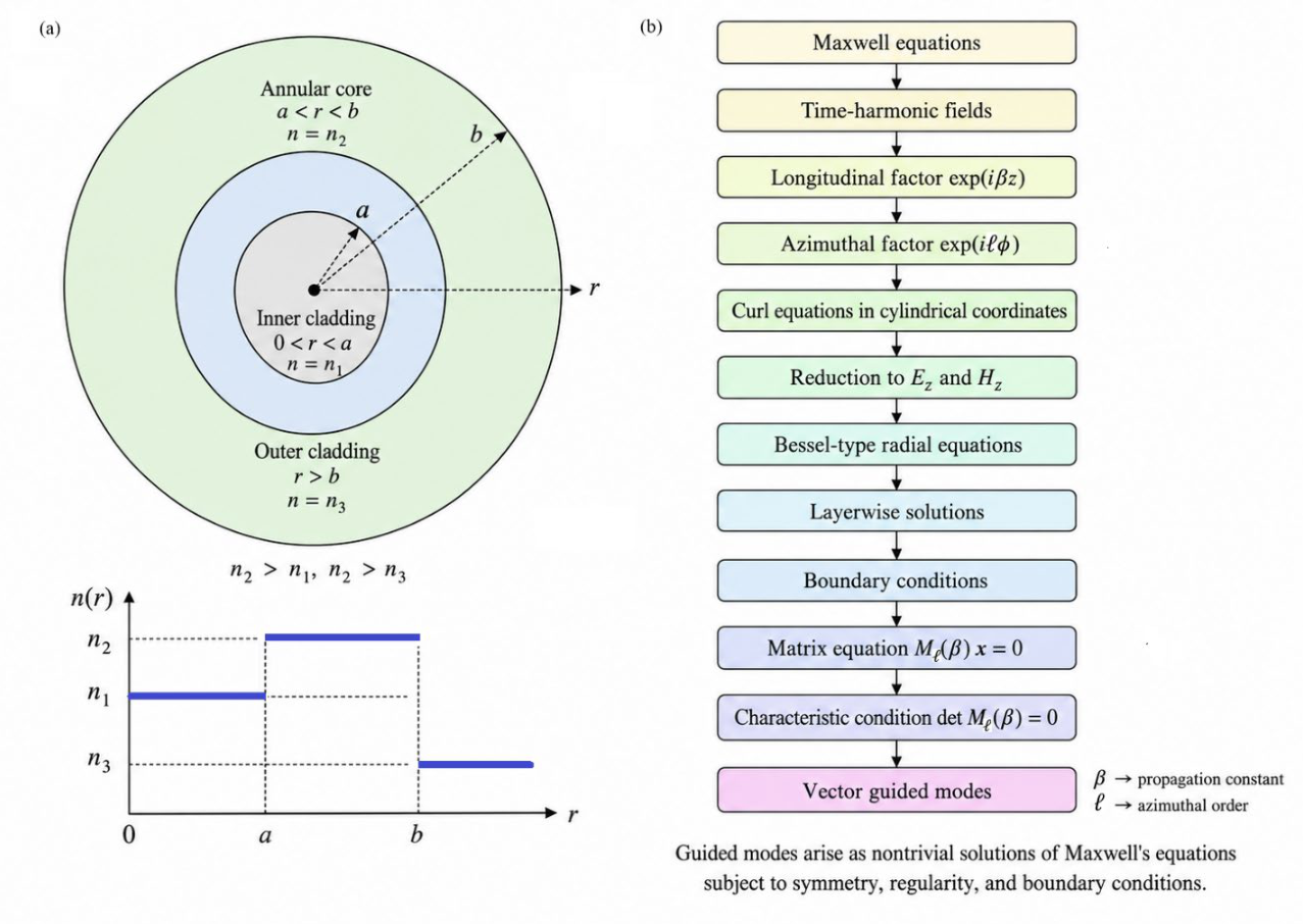
Figure 2.
Physical interpretation of modal quantities in a ring-core fiber. (a) The propagation constant β determines the longitudinal phase accumulation of a guided mode through the factor . (b) The effective refractive index lies between the refractive indices of the cladding regions and the high-index annular core for a bound ring-core mode. (c) The azimuthal order determines the angular phase factor : corresponds to an azimuthally phase-uniform, non-vortex mode, whereas and illustrate vortex-compatible phase winding. (d) Radial localization describes the concentration of modal intensity in the annular guiding region . (e) The Poynting-flux localization factor quantifies the fraction of guided power carried inside the annular core.
Figure 2.
Physical interpretation of modal quantities in a ring-core fiber. (a) The propagation constant β determines the longitudinal phase accumulation of a guided mode through the factor . (b) The effective refractive index lies between the refractive indices of the cladding regions and the high-index annular core for a bound ring-core mode. (c) The azimuthal order determines the angular phase factor : corresponds to an azimuthally phase-uniform, non-vortex mode, whereas and illustrate vortex-compatible phase winding. (d) Radial localization describes the concentration of modal intensity in the annular guiding region . (e) The Poynting-flux localization factor quantifies the fraction of guided power carried inside the annular core.
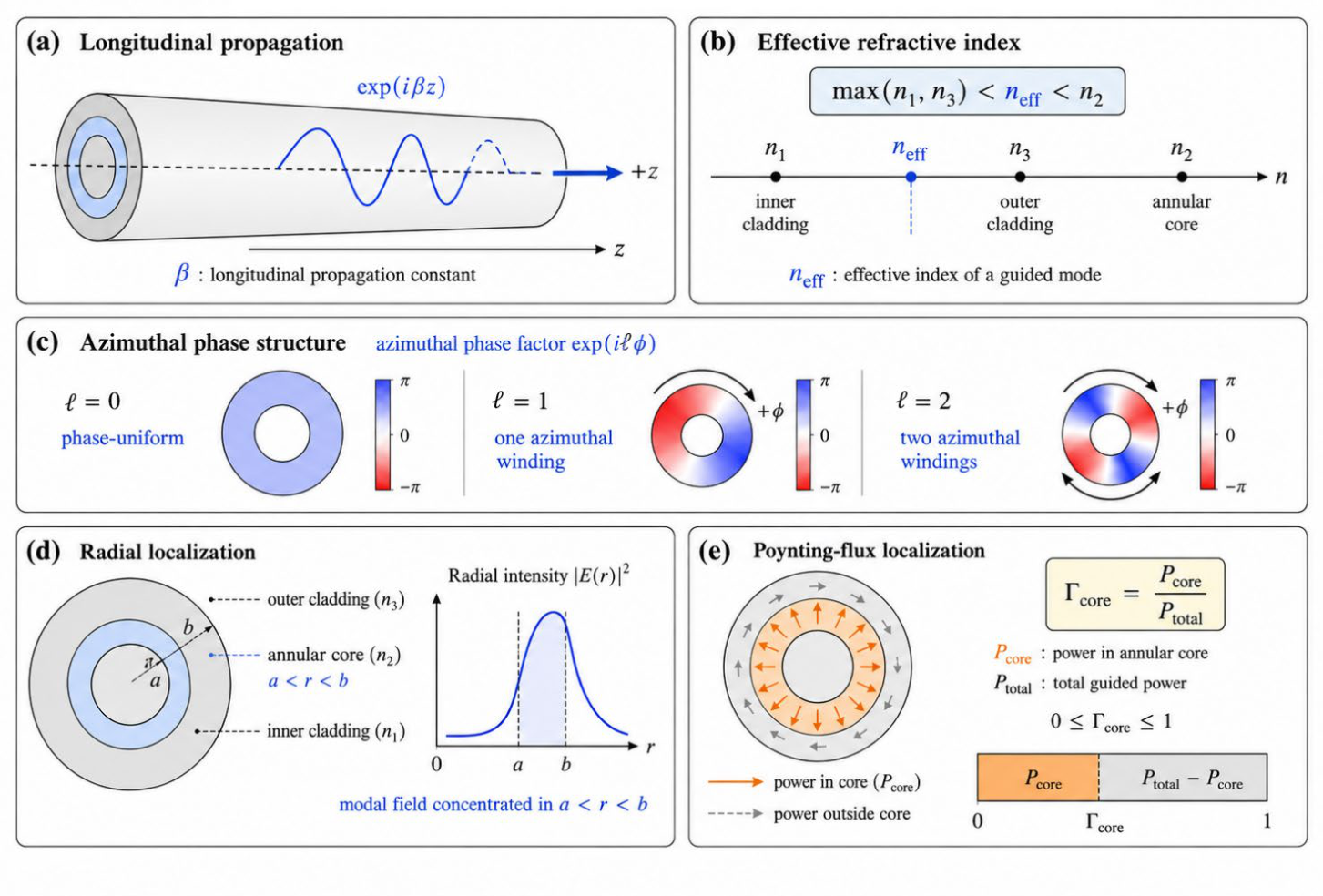
Figure 3.
Radial profiles of representative ring-core guided modes. Schematic radial amplitudes for representative modes with azimuthal orders = 0, = 1, and = 2. The dashed vertical lines mark the inner and outer boundaries of the annular core, and , while the shaded region indicates . The amplitudes are shown on a common arbitrary scale and are intended only as schematic profiles rather than optimized numerical eigenmodes.
Figure 3.
Radial profiles of representative ring-core guided modes. Schematic radial amplitudes for representative modes with azimuthal orders = 0, = 1, and = 2. The dashed vertical lines mark the inner and outer boundaries of the annular core, and , while the shaded region indicates . The amplitudes are shown on a common arbitrary scale and are intended only as schematic profiles rather than optimized numerical eigenmodes.
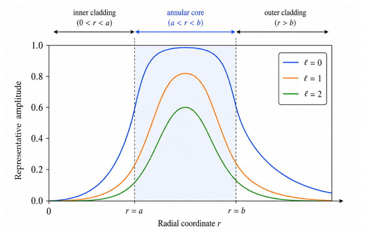
Figure 4.
Intensity and phase maps for representative azimuthal orders. Schematic transverse intensity and phase maps for representative ring-core guided modes with azimuthal orders , , and . The intensity maps show annular localization of the modal field in the ring-core region between the inner radius and outer radius . The phase maps illustrate the azimuthal phase structure of a selected complex field component, for example . For , the mode has annular intensity but no azimuthal phase winding; it is therefore a phase-uniform, non-vortex annular mode. For and , the phase winds once and twice around the fiber axis, respectively, corresponding to vortex-compatible guided states. The figure emphasizes that annular intensity alone does not imply vortex phase: radial localization is determined by the ring-core refractive-index profile, whereas azimuthal phase winding is determined by the factor . The maps are representative and normalized for visual comparison.
Figure 4.
Intensity and phase maps for representative azimuthal orders. Schematic transverse intensity and phase maps for representative ring-core guided modes with azimuthal orders , , and . The intensity maps show annular localization of the modal field in the ring-core region between the inner radius and outer radius . The phase maps illustrate the azimuthal phase structure of a selected complex field component, for example . For , the mode has annular intensity but no azimuthal phase winding; it is therefore a phase-uniform, non-vortex annular mode. For and , the phase winds once and twice around the fiber axis, respectively, corresponding to vortex-compatible guided states. The figure emphasizes that annular intensity alone does not imply vortex phase: radial localization is determined by the ring-core refractive-index profile, whereas azimuthal phase winding is determined by the factor . The maps are representative and normalized for visual comparison.
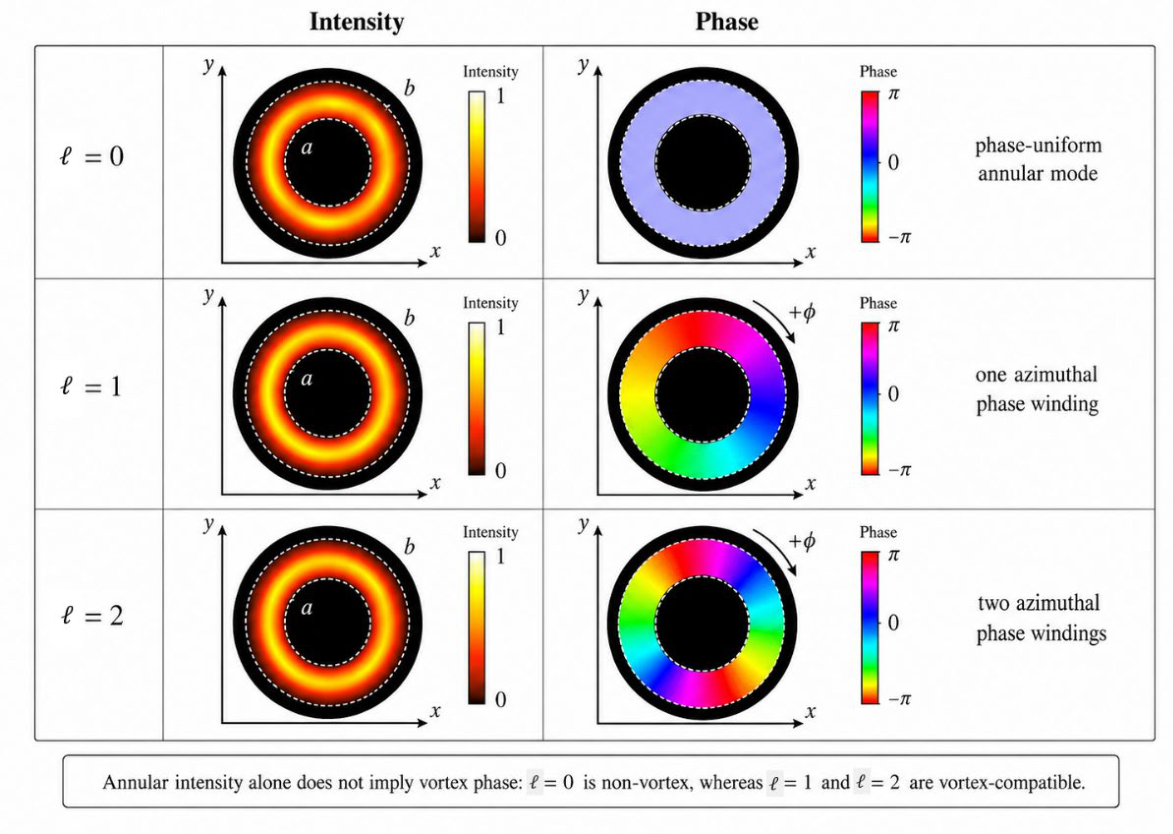

Table 1.
Computed modal quantities for the illustrative parameter set.
| Mode branch | β, µm⁻¹ | Interpretation | ||||
| 0 | 1 | 1.4636 | 5.933 | 0.924 | < 10⁻¹⁰ | phase-uniform annular mode |
| 1 | 1 | 1.4642 | 5.935 | 0.921 | < 10⁻¹⁰ | one azimuthal phase winding |
| 2 | 1 | 1.4635 | 5.933 | 0.923 | < 10⁻¹⁰ | two azimuthal phase windings |
Table 2.
Power-normalized expansion coefficients for the representativevector mode.
| Coefficient | Real part | Imaginary part | Associated longitudinal field and region |
| | 7.0264× | 0 | , inner cladding |
| 0 | −1.0866× | , inner cladding | |
| | 1.05461× | 0 | , annular-core term |
| −1.10528× | 0 | , annular-core term | |
| | 0 | −1.63693× | , annular-core term |
| | 0 | 1.62619× | , annular-core term |
| −30.8063 | 0 | , outer cladding | |
| | 0 | 46.0417 | , outer cladding |
Disclaimer/Publisher’s Note: The statements, opinions and data contained in all publications are solely those of the individual author(s) and contributor(s) and not of MDPI and/or the editor(s). MDPI and/or the editor(s) disclaim responsibility for any injury to people or property resulting from any ideas, methods, instructions or products referred to in the content. |
© 2026 by the authors. Licensee MDPI, Basel, Switzerland. This article is an open access article distributed under the terms and conditions of the Creative Commons Attribution (CC BY) license (http://creativecommons.org/licenses/by/4.0/).
Copyright: This open access article is published under a Creative Commons CC BY 4.0 license, which permit the free download, distribution, and reuse, provided that the author and preprint are cited in any reuse.