

Submitted:
11 July 2026
Posted:
13 July 2026
You are already at the latest version
Abstract
This paper proposes a spatial‑functional two‑dimensional hierarchical group decision‑making (HGDM) spectrum management architecture for emergency communication unmanned aerial system (EC‑UAS). The architecture handles the highly dynamic topology, large node population, and differentiated task priorities that characterize EC‑UAS. Using the spectrum management properties of EC‑UAS, we develop a discrete‑time closed‑loop dynamic model of the architecture and design adaptive hierarchical iteration rules. We prove global stability of the model under the stated assumptions and analyze the convergence of the state error, deriving its theoretical upper bound and the relationship between convergence steps and accuracy. An input‑to‑state stability analysis further demonstrates that the system state error remains bounded under dynamic disturbances, with its magnitude scaling with the disturbance bound. Simulations verify the effectiveness of the architecture and the correctness of the theoretical analysis.
Keywords:
emergency communication UAV swarms (EC‑UAS)
; spectrum management
; hierarchical group decision-making (HGDM)
; spatial‑functional two‑dimensional architecture
1. Introduction
As aerial communication base stations for post-disaster emergency rescue, Emergency Communication UAV Swarms (EC-UAS) provide temporary communication coverage through multi-UAV collaborative networking. Owing to their rapid deployment, wide coverage, and strong adaptability to complex terrains, EC-UAS have become a critical support for post-disaster emergency communication [1,2]. Meanwhile, the highly dynamic topology, large number of nodes, and differentiated task priorities of EC-UAS pose new challenges for multi-UAV communication and control. The high-speed movement of UAVs causes the spectrum environment to change rapidly, and the available frequency bands remain effective only for a short time. It is necessary to complete the spectrum state perception and frequency usage decision-making in a very short time [2,3,4]. In a large-scale swarm, nodes simultaneously compete for limited spectrum resources. If each node independently performs global optimization, the computational and communication overhead will increase sharply with the number of nodes. The frequency usage coordination must keep the overhead controllable when the node scale grows [5,6]. Post-disaster emergency rescue nodes are generally fragile and resource-constrained. Node failures and link faults are likely to lead to spectrum resource waste and new frequency usage conflicts. The spectrum management framework needs to instantly optimize frequency usage plans and dynamically resolve conflicts. [7,8]. In addition, multiple types of tasks run in parallel in emergency scenarios. Allocating spectrum resources according to task priorities ensures that low-priority tasks do not preempt the frequency requirements of high-priority ones [9,10].
The architecture for spectrum management and control is the core of EC-UAS operations. It generally falls into three categories: centralized, distributed, and hybrid. In a centralized architecture, a global central node collects status information from all nodes and handles the global allocation of spectrum resources. This architecture can achieve global optimality in small-scale scenarios. As the swarm expands, the computing and communication overhead of the central node grows. A single failure of this node can paralyze the entire management and control system [1]. In a distributed architecture, UAV nodes handle sensing and decision-making locally, and they coordinate spectrum usage through local information exchange. It offers good scalability and fault tolerance. Without global spectrum information, nodes in a distributed architecture often converge to local optima when making autonomous decisions. In highly dynamic scenarios, a distributed architecture can easily lead to spectrum usage conflicts between sub-clusters [3,11]. The hybrid architecture is a combination of the first two types of architectures. Typical implementations include partitioning the swarm into sub-clusters with designated head nodes [10], hierarchical decision-making via proximal policy optimization [12], and collaborative intelligent networking for UAV swarm emergency communications [13,14]. In existing hybrid architectures, sub-cluster head nodes essentially relay information; local conflict decisions are still resolved by the global node. Consequently, their adaptability to dynamic topologies remains limited [15,16].
Hierarchical group decision-making (HGDM) coordinates large-scale intelligent groups by structuring them into multiple correlated subsystems. Global optimal decisions emerge from coordination across these levels [17]. Bidram et al. applied HGDM in microgrid control, distributing control tasks across levels by response speed. The bottom layer handles millisecond-level voltage and current regulation decisions, the middle layer makes minute-level frequency recovery decisions, and the top layer performs hour-level economic dispatch [18]. Building on this, Guerrero et al. delegated power sharing and allocation at the unit level to the bottom-layer control system, and assigned system-level voltage recovery (both its timing and method) to the top layer [19]. In transportation, Shen applied HGDM to traffic signal control by separating decision-making authority from plan execution. The upper-level system sets the regional traffic goals, and lower-level intersections independently generate their own signal timing schemes, achieving a balance between global coordination and local responsiveness [20].
In UAV swarm control, Meer et al. used HGDM to design a control strategy that delegates dynamic reconfiguration to the edge cloud and power control to the access point [16]. Sun used proximal policy optimization to design a hierarchical action space for downlink time-frequency resource allocation in UAV base stations. This method decomposes the global multi-channel problem into per-channel sub-problems and solves them sequentially, improving decision-making efficiency in large-scale networks [12]. Ref. [13] proposed an intelligent collaboration method based on team Markov games for multi-UAV swarm trajectory planning. The work designed a Q-function mixed network (QMIX) architecture and used a hierarchical decision-making mechanism combining global value mixing and local policy execution to achieve wireless coverage of ground users. In heterogeneous scenarios with spectrum sharing requirements, Liao et al. let the head node handle coordination and member nodes handle frequency selection, effectively reducing mutual interference during spectrum use [14].
In EC-UAS spectrum management, the HGDM architecture offers clear advantages. Each level can resolve frequency-use conflicts independently and only needs to report global conflicts to the top level for coordination, greatly reducing the burden on top-level nodes. When resolving frequency-use conflicts, it gives priority to high-priority tasks, providing differentiated protection across priority levels. Each level reports conflicts only when needed, significantly reducing the communication overhead in large-scale clusters. To address these challenges, the main contributions of this paper are as follows:
This paper presents a space–function two-dimensional HGDM architecture for spectrum management. A discrete-time closed-loop dynamic model and adaptive hierarchical iteration rules are developed for the architecture, followed by theoretical analysis and experimental validation. The main contributions are summarized as follows:
- A space–function two dimensional HGDM architecture for spectrum management and control in EC UAS.
- A discrete time closed loop dynamic model with adaptive hierarchical iteration rules.
- Proofs of global stability, convergence rate bounds, and robustness under bounded disturbances.
The remainder of this paper is organized as follows. The EC-UAS system model is formulated in Section 2, where three types of spectrum conflicts are defined and the layered multi-node mathematical foundation is established. Section 3 describes the space–function two-dimensional HGDM architecture, covering the adaptive decision-triggering mechanism and the discrete-time closed-loop dynamic model. Proofs of global asymptotic stability, exponential convergence, and input-to-state stability under bounded disturbances are provided in Section 4. Numerical results and discussion are presented in Section 5, and Section 6 concludes the paper.
2. Problem Formulation
In major disasters such as earthquakes and floods, EC-UAS rapidly builds a communication network to support real-time collaboration among tasks with different priorities, including life detection, rescue instruction transmission, and material scheduling. An EC-UAS typically consists of multiple sub-clusters, each deployed in a distinct area: the core rescue area, the collaborative support area, the global coverage area, and the material transfer area [22,23]. Each sub-cluster contains several UAVs equipped with communication and spectrum sensing capabilities. The task priorities differ not only across sub-clusters but also among the UAVs within the same sub-cluster, as shown in Figure 1.
EC-UAS faces three types of spectrum usage conflicts, distinguished by their scope and impact [24]. Intra-cluster conflicts arise from spectrum allocation and resolution among nodes within a single cluster. Inter-cluster conflicts stem from mutual interference between sub-clusters where their coverage areas overlap. Global conflicts involve complex, cross-regional interactions across multiple clusters, and resolving them requires coordinated linkage to maintain efficient data transmission and task collaboration throughout the system. Because both spectrum resources and task requirements change rapidly in EC-UAS scenarios, the decision-making mechanism for spectrum management must adapt accordingly, responding in a differentiated way to distinct conflict types and task requirements while ensuring communication continuity for high-priority tasks as the topology evolves.
HGDM is well suited to EC-UAS because its design aligns with the swarm’s hierarchical structure, its multi-agent decision requirements, the conflict-intensive nature of the environment, and the need to differentiate among task priorities. The node–sub-cluster–cluster organization naturally maps to a layered perception–decision–execution architecture, reinforced by the classification of spectrum conflicts into intra-cluster, inter-cluster, and global types. Group decision-making follows from the multi-agent characteristics of EC-UAS and the collaborative demands of spectrum management; the strategies employed range from intra-group autonomy and inter-group collaboration to swarm-wide consensus. The decision logic is explicitly conflict-oriented, reflecting the close link between spectrum conflicts and mission tasks, and it establishes a clear mapping between strategies and the conflicts they address. Task-priority differentiation is embedded throughout, ensuring that high-priority tasks receive preferential spectrum access in both the decision logic and the strategy–priority mapping.
For the convenience of research, the EC-UAS is abstracted as a cluster composed of N UAV nodes. The nodes are divided into K sub-clusters according to spatial distribution and task association. The k-th sub-cluster is denoted as , which satisfies and the sub-clusters are pairwise disjoint. The sub-cluster has a head node, which is responsible for aggregating the status information of member nodes within this sub-cluster. This node participates in the collaborative decision-making across sub-clusters. The communication topology of the entire network is described by an undirected graph , with the node set and the edge set representing the links through which nodes can directly communicate. To ensure that information can spread across the whole network within a finite number of steps, remains connected at any time. The spectrum management action of EC-UAS is abstracted as a discrete-time process, and the sampling time is denoted as . Each i node maintains a state vector at time t, representing the current globally optimal frequency-usage plan. This state vector can encode information such as spectrum occupancy vectors, transmit power configurations, and channel selections. In theoretical analysis, to maintain the generality of the model, the state vector is abstracted as a multi-dimensional state variable. Each node is assigned a task priority. Nodes corresponding to high-priority tasks have a larger step size, ensuring that their spectrum allocation estimates converge to the globally optimal solution preferentially at the dynamic level.
3. Hierarchical Group Decision-Making Framework
3.1. Spatial-Functional Two-Dimensional Architecture
The space–function two-dimensional HGDM architecture for EC-UAS spectrum management consists of two complementary dimensions, as shown in Figure 2. The left side represents the spatial dimension, which clarifies the physical distribution and organizational hierarchy of nodes and forms a decision-making chain that follows the logic of local autonomy, regional coordination, and global planning. The right side represents the functional dimension, where the spectrum management tasks are assigned to the corresponding spatial levels. This separation of spatial boundaries from functional execution allows the architecture to keep decision-making authority, capabilities, and scope precisely aligned even as the topology changes and the network expands.
Each spatial level hosts a set of functional entities with distinct responsibilities. At the bottom, spectrum-using nodes (SN) serve as the sensing and execution terminals of the system. They sense the local spectrum environment, select frequency bands autonomously, adjust transmit power, and report their status to the upper layer. The middle layer consists of sub-cluster head nodes (SHN), which aggregate and filter the status information from member nodes, handle spectrum allocation within their sub-clusters, and trigger adaptive decisions when needed. These nodes bridge the upper and lower levels by providing data fusion and regional coordination. The top-layer global control nodes (GCN) work as the decision-making centers for global sensing and overall planning. They resolve spectrum conflicts that span multiple sub-clusters, coordinate global spectrum resources, and assign priority to high-priority tasks.
3.2. Hierarchical Group Decision-Making Method
HGDM divides spectrum management into two stages: strategy selection and decision implementation. The first stage groups strategies by conflict scope into three types—within-group, between-group, and global—and delegates each type to the corresponding level in the spatial hierarchy. The second stage uses the bidirectional links defined by the architecture to pass information between levels, enabling entities at each level to switch strategies and adjust spectrum usage through mutual coordination.
3.2.1. Strategy Selection
Three real-time indicators from the perception layer—conflict intensity, topological dynamics, and task priority—jointly drive adaptive decision-making and strategy switching. The Conflict Quantification Index (CQI) measures the severity and spatial reach of spectrum conflicts. It combines the frequency occupancy rate and interference intensity into a weighted value in [0,1], and this value determines which hierarchical level should resolve a given conflict. The Topological Dynamics Index (TDI) captures topology stability from node movement speeds and link connectivity changes, yielding a value in [0,1] that indicates how strongly topology dynamics should influence decision-making. The Task Priority Weight (PW) expresses a task’s urgency and life-criticality, derived from its life-related degree and rescue time sensitivity; its value, also in [0,1], is used to prioritize high-priority tasks for spectrum access. The real-time values of these three indicators trigger a stepwise strategy-selection procedure, as shown in Figure 3.
When CQI<0.5 and TDI≤0.6, conflict intensity is low and the topology is stable. The system uses an intra-swarm autonomous consensus strategy, and SN nodes resolve conflicts through distributed negotiation, with no cross-layer information exchange.
When 0.5≤CQI<0.7 and TDI≤0.6, conflicts extend across sub-swarms while the topology remains stable. The system switches to an inter-swarm collaborative game strategy, and SHN nodes coordinate cross-region resources via state synchronization and payoff balancing.
When CQI≥0.7 or TDI>0.6, conflicts become global or the topology becomes highly dynamic. The system activates a swarm-wide coordination strategy, and the GCN node performs unified resource scheduling across the entire network.
Independently, if PW≥0.8, a dedicated high-priority task protection process takes precedence. It locks low-interference frequency bands and reserves flexible resources for core rescue tasks, regardless of the other indicator values.
3.2.2. Strategy Implementation
At the decision-execution level, a strategy switch is carried out in three stages to avoid unnecessary switching triggered by transient fluctuations.
Stage I: On receiving a switch instruction, the system immediately reserves temporary spectrum resources for the conflicting nodes, so that existing communication links remain operational.
Stage II: The relevant decision-making entities then take actions according to the strategy level. When the intra-cluster autonomous collaboration strategy is active, SN nodes exchange local state information and adjust channel selection and transmit power. For the inter-cluster collaborative game strategy, SHN nodes negotiate a cross-region spectrum partition plan step by step and distribute it to the subordinate SN nodes. When swarm-wide coordination is invoked, the GCN node generates an optimization plan based on the global state and transmits it layer by layer through the SHN nodes.
Stage Ⅲ: After the strategy is executed and the spectrum configuration stabilizes, the system collects CQI, TDI, and PW a second time. If the indicators return to the stable range and the conflict has been resolved, the switching process ends. If the triggering conditions are still met, the system re-enters the strategy-selection and execution cycle until the frequency-use conflict of the EC-UAS is resolved.
3.3. Closed-Loop Dynamic Model
3.3.1. Hierarchical State Update Equation
Assumption 1 (Connectivity):
The communication topology of the EC-UAS system is strongly connected. For any pair of nodes i and j, there exists at least one communication path between them, through which information exchange can be completed either directly or via relays.
Assumption 2 (Bounded step sizes):
The update step sizes of the system are , , and , where is a constant, and this holds for all i, k, and t.
According to the spatial distribution and task association relationship, the nodes of the EC-UAS system are divided into K sub-clusters. Denote the k-th sub-cluster as , with the number of nodes being . Each node i maintains a state vector at time t, representing its current estimate of the global optimal spectrum allocation scheme. Each sub-cluster has a head node, which is responsible for state aggregation within the sub-cluster. The system operation is modeled as a discrete-time process . The proposed HGDM architecture can be abstracted as a discrete-time hierarchical state update rule
In which, represents the number of nodes in sub-cluster . The GCN nodes further fuse the aggregated states of all sub-clusters to obtain the global system state:
In which, K represents the total number of sub-clusters in the system. can be regarded as the system's current estimate of the global optimal spectrum allocation scheme at time t. Based on the above aggregated information, the system's state update follows the following three-layer hierarchical rules. The core idea is to enable decision-making entities at different levels to gradually approach the global optimal state through consensus iteration within their own control scopes.
The SN node i of the EC-UAS system updates its own state according to the aggregation state of the sub-cluster it belongs to
In which is the update step size, which is adaptively adjusted according to the task priority weight PW of node i. When PW is relatively large, increases accordingly, and the nodes of high-priority tasks move closer to the sub-cluster consensus state to a greater extent, thus achieving the priority convergence of core rescue tasks.
The SHN node k of the EC-UAS system updates the aggregated state of its sub-cluster according to the global system state.
In which, represents the update step size, which is adaptively adjusted according to the topological dynamic index (TDI) of the sub-cluster. When the topological change accelerates, increases accordingly to ensure rapid tracking of the dynamic environment.
The GCN nodes of the EC-UAS system adjust the global system state based on the global optimal state estimation
In which, is the update step size, which is adaptively adjusted according to the global conflict quantification value CQI. When the conflict intensity increases, increases accordingly to accelerate the resolution of global conflicts. is the estimated value of the global optimal state at the current moment, which can be calculated by GCN according to the global spectrum occupancy state and task priority distribution in the actual system, and a constant value is taken in the simulation.
3.3.2. Closed-Loop Dynamic Equations
Equations (1)-(5) together constitute a closed-loop dynamic model for the HGDM framework. To characterize the overall dynamic behavior of the system, let the stacked vector of all node states be , and the stacked vector of all sub-cluster aggregated states be . The complete evolution of the system can be further expressed as:
In which, is the system state transition matrix, and its elements are jointly determined by the update step size in Eqs. (3)-(5); is the input matrix dependent on the global step size , which characterizes the guiding effect of the global optimal state on the state update of each layer.
4. Theoretical Analysis
4.1. Stability and Convergence
Theorem 1 (Stability):
Under the conditions of Assumption 1 and Assumption 2, let the global optimal state estimate be a constant value
. Then the hierarchical state update system defined by Eqs. (1)-(5) is asymptotically stable. That is, for any initial state
, holds for all
.
Proof:
To analyze the stability of the system, the following Lyapunov function is defined:
This function corresponds to the sum of the squares of the errors between the local states of all nodes and the global optimal state. Obviously, there is , and . Consider the variation of along the system trajectory . Substituting the state update equation (3), for node i belonging to subset group :
Combining the subset group state definition (1) and the global state update equation (4)-(5), it can be concluded that there exists a constant that:
In which, is the system convergence factor. According to Hypothesis 2, all step sizes belong to (0,1), so .
Therefore, for any t, there is , indicating that is monotonically non-increasing. According to Lyapunov's stability theorem, the system is asymptotically stable. Verified #
Theorem 1 guarantees that the system will inevitably converge to the global optimal solution under any initial conditions, theoretically eliminating the risk of architecture failure due to state divergence.
Theorem 2 (Convergence):
Under the conditions of Hypothesis 1 and Hypothesis 2, the state error of the system converges to zero at an exponential rate. That is, for any
, there is:
In which, is the sum of the squares of the initial state errors. For any given convergence accuracy , the upper bound of the number of steps required for the system to achieve convergence is:
In which, represents the initial state error, and is the convergence factor of the system.
Proof: As can be seen from Equation (8), the Lyapunov function satisfies the difference inequality:
From , it can be concluded that decays exponentially with over time. For the given convergence precision , when , there is
Therefore, the upper bound of the number of steps required for convergence is shown in Equation (10). Verified #
Theorem 2 reveals a key property of the system's convergence rate, that is, the number of convergence steps is only proportional to the logarithm of the convergence accuracy, rather than being a power function of . This means that even if extremely high convergence accuracy is required, the system only needs a few additional iterations to achieve it, demonstrating the typical fast convergence characteristics of large-scale networks.
4.2. Robustness Analysis Under Dynamic Disturbances
Affected by bounded disturbances such as communication noise, node measurement errors, and local decision biases, the local update equation (3) of the SN node of EC-UAS is rewritten as:
In which, is the perturbation vector that node experiences at time . Suppose the perturbation is bounded, that is, there exists a constant such that for all and , there is .
Inference 1 (Input-state stability):Under the conditions of Hypothesis 1 and Hypothesis 2, the disturbed hierarchical system defined by equations (1)-(2), (4)-(5), and (11) is input-state stable. That is, there exists a KL-class function and a K-class function such that for any bounded perturbation sequence
, the system state error satisfies:
Proof:
According to the ISS theory, for discrete-time nonlinear systems, if there exists an ISS-Lyapunov function in the undisturbed state, the system is input-state stable. As proved by Theorem 1, under undisturbed conditions, function satisfies:
When disturbance exists, substitute equation (11) into . The cross-terms that appear after expansion will consume part of the attenuation margin when scaled by algebraic inequalities, making the effective attenuation factor of the disturbed system slightly less than without disturbance. From this, it can be concluded that there exist constants and that satisfy:
In which, is generated by scaling and contracting the upper bound of the perturbation, and is the perturbation gain constant determined by the upper bound of the system dimension and step size, reflecting the degree to which the perturbation amplifies the state error. Equation (13) indicates that when the state error is large, , strictly decays. When the error has converged to the neighborhood determined by , . May grow bounded but will not diverge. The form of equation (12) can be obtained by iterating from equation (13). Verified #.
Inference 1 indicates that when a system is subjected to bounded disturbances, the state error is not continuously magnified to diverges but is confined within the neighborhood bounded by . This means that even under harsh working conditions such as a decline in communication quality and temporary failure of some nodes, the system can still control the deviation of the spectrum allocation scheme within an acceptable range.
The adaptive adjustment of step size in the HGDM mechanism further enhances the robustness of the architecture in perturbation scenarios. When the topological dynamics index (TDI) increases, the update step size of the SHN node adaptively increases by , accelerating the tracking of the state changes of this subset group and offsetting the disturbances introduced by the rapid topological changes. When the conflict quantization value CQI increases, the update step size of GCN nodes adaptively increases, accelerating the resolution of global conflicts and suppressing the cascading disturbances caused by the spread of conflicts. When the task priority weight PW increases, the update step size of the SN node adaptively increases, accelerating the convergence of high-priority tasks and reducing the accumulated deviation caused by the long queuing of high-priority tasks. The above-mentioned triple adaptive adjustment mechanism enables the system to actively adjust the convergence speed in response to dynamic disturbances, rather than passively waiting for a slow recovery with a fixed step size. This theoretically explains the superiority of the adaptive hierarchical triggering mechanism proposed in Section 3.
5. Simulation Verification and Analysis
A simulation platform was developed based on Python 3.10 and NumPy. Six experiments were designed to evaluate: convergence behavior, step-size influence, convergence verification, disturbance response, node failure recovery, and the impact of topological dynamics on the HGDM architecture and the closed-loop model (see Eq. (6) in Section 3.3).
5.1. Simulation Environment Settings
The abstract state consensus model is adopted, and the core parameters are set as follows: the number of unmanned aerial vehicle nodes N=50, the number of subset groups K=5, each subset group contains 10 nodes, and the dimension of the state vector d=3. The global optimal spectrum allocation scheme is set to , and the initial states of each node are randomly generated within [0,1]³. The task priority weights are allocated in three levels: high, medium and low, with the weight values set at 0.8, 0.5 and 0.2 respectively. Within each subset group, a configuration of approximately 2 high-priority nodes, 4 medium-priority nodes and 4 low-priority nodes is adopted, and the node order is shuffled by a fixed random seed to ensure the reproducibility of the results.
Set two schemes: the adaptive step size scheme and the fixed step size scheme. The adaptive step size scheme adopts hierarchical adaptive rules. According to the adaptive mechanism described in Section 3.3, the step size is jointly determined by the node priority PW, the topological dynamics index TDI, and the conflict quantization value CQI. Specifically, the following calculation formula is used: ,,. In which, is the priority coefficient of node i, and the values of the high, medium and low levels are 0.8, 0.5 and 0.2 respectively. The base step size is set to 0.3 by default (it will be changed when studying its impact in Experiment Two). The fixed step size scheme is used as the comparison benchmark, and all step sizes are uniformly set to . The root mean square error is adopted as the evaluation index
It is used to measure the degree of deviation between the global state and the optimal solution.
5.2. Robustness Analysis Under Dynamic Disturbances
Experiment 1: Convergence Verification
To verify the stability stated in Theorem 1, both the adaptive and the fixed step-size schemes were run for 500 steps each under standard conditions—no external disturbances, with TDI = CQI = 0.3. Figure 4 shows their RMSE convergence curves from the same initial state.
Figure 4 shows that both schemes can make RMSE converge to nearly zero, verifying the stability of the system under standard conditions. When RMSE drops to 1×10⁻³, the adaptive scheme requires approximately 30 steps, while the fixed-step scheme requires about 120 steps. The adaptive scheme converges faster, which is attributed to its differentiated assignment step size based on the node priority coefficient, enabling high-priority nodes to approach the optimal state with a greater update amplitude, thereby accelerating the overall convergence of the system.
Experiment 2: The Influence of Step Size
Five values of the reference step size were chosen to examine its impact on the convergence speed. For each value, 10 independent runs were performed, and the mean and standard deviation of the number of steps needed for RMSE to drop to 1×10⁻³ were recorded. Figure 5 summarizes the results.
Figure 5 shows the average convergence steps under different reference step sizes, plotted in logarithmic coordinates. For a = 0.1, 0.2, 0.3, 0.4, and 0.5, the average steps are 2034.5, 253.2, 73.9, 30.4, and 14.8. A larger step size accelerates convergence, but an overly large value weakens the system’s ability to suppress high-frequency disturbances. In practice, a compromise is needed between convergence speed and steady-state accuracy.
Experiment 3: Verification of Exponential Convergence
To verify the convergence property described in Theorem 2, the RMSE curve is plotted on semi-logarithmic coordinates, and a theoretical upper bound constructed from the spectral radius of the closed-loop update matrix is superimposed. Figure 6 shows the resulting attenuation trajectories.
Figure 6 shows the RMSE attenuation trajectories together with the theoretical upper bounds for the adaptive and fixed-step schemes. On semi-logarithmic axes, both curves decay roughly linearly, consistent with the exponential convergence predicted by theory. The adaptive scheme exhibits a steeper slope, reflecting its faster convergence. The upper bound derived from the spectral radius of the closed-loop update matrix (ρ≈0.973) tightly bounds the RMSE and confirms the conclusion of Theorem 2 on the upper limit of convergence steps.
Experiment 4: Robustness under External Sudden Disturbances
To evaluate the ISS property in Inference 1, the system first ran stably to t = 200. Gaussian disturbances (σ = 0.5) were then applied to 30 % of the nodes for six consecutive steps, after which the disturbance was removed and the recovery process was observed. The complete response is shown in Figure 7.
Figure 7 shows the complete disturbance response curve. During the disturbance, the RMSE peaks of the adaptive and fixed-step schemes reached about 0.814 and 0.862, respectively. The error rose sharply but stayed bounded and never diverged. After the disturbance stopped, the adaptive scheme recovered to within 1 × 10⁻³ by step 293, while the fixed-step scheme required step 388. These results demonstrate the system’s robustness under bounded external disturbances: the error remains bounded throughout, and the system recovers on its own once the disturbance is removed. The adaptive scheme regains stability faster because of its dynamic step-size adjustment.
Experiment 5: Robustness under random node failure
To assess robustness against sudden topological changes, 20 % of the nodes (10 out of 50, including one sub-cluster head) were randomly removed at t = 200. The failed nodes no longer participate in state aggregation and updates. A small state perturbation was then applied to the remaining nodes of the affected sub-cluster to mimic the transient impact of head re-election. Figure 8 shows the response under this failure scenario.
Figure 8 shows the response curves of the two schemes, with a magnified inset highlighting the moment of failure. At the failure instant, the RMSE values of the adaptive and fixed schemes are approximately 0.01543 and 0.01542, respectively. After the failure, the adaptive scheme recovered to within 1 × 10⁻³ at step 227, while the fixed scheme required step 258. These results indicate that even when some nodes (including a sub-cluster head) suddenly fail, the architecture can continue operating on the remaining nodes and gradually return to stability. This confirms the effectiveness of the hierarchical fault-tolerance mechanism described in Section 3.2.2 in practical scenarios.
Experiment 6: The Influence of topological Dynamics on Steady-state Performance
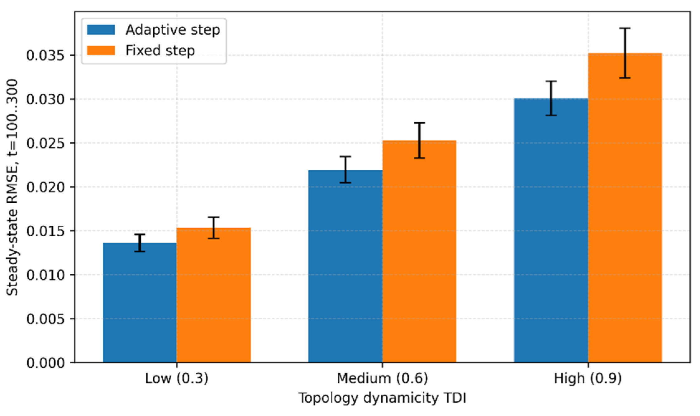
Three TDI levels, 0.3 (low), 0.6 (medium), and 0.9 (high), were used to simulate different degrees of topology dynamics. Each setup ran for 300 steps, and the steady-state RMSE was computed as the mean from t = 100 to 300. A bounded topological perturbation that increases with TDI was added to reflect the state fluctuations caused by frequent link on-off in real scenarios. The results are presented in Figure 9.
Figure 9 compares the steady-state RMSE of the adaptive and fixed-step schemes under three TDI levels. As TDI grows, the steady-state error of both schemes increases, indicating that higher topology dynamics degrade tracking accuracy. The adaptive scheme consistently achieves a lower RMSE across all three conditions, with relative reductions of about 11.19% (TDI = 0.3), 13.28% (TDI = 0.6), and 14.68% (TDI = 0.9). These results suggest that the adaptive step-size mechanism can partially offset the tracking deviations introduced by topological changes through dynamic adjustment of the update amplitude. The improvement becomes more pronounced as the topology becomes more dynamic, confirming the advantage of the proposed adaptive hierarchical triggering mechanism in highly dynamic scenarios.
6. Conclusion
This paper has proposed a space–function two-dimensional HGDM spectrum management architecture for EC-UAS. A discrete-time closed-loop dynamic model was established, and Lyapunov stability theory together with input-to-state stability theory were used to prove the stability, convergence, and robustness of the architecture. A quantitative relationship between convergence rate and the theoretical error bound was also derived. Simulation results show that the adaptive step-size scheme reduces the convergence steps by roughly three quarters compared with a fixed step-size scheme. Under external disturbances and node failures, the system error remains bounded and recovers quickly. In highly dynamic topology scenarios, the steady-state error of the adaptive scheme is 11%–15% lower than that of the fixed scheme, confirming the effectiveness and reliability of the architecture under typical EC-UAS operating conditions. Future work will combine conflict pre-sensing with dynamic resource allocation to further improve the architecture’s adaptability in extreme scenarios.
Author Contributions
Conceptualization, Hengzhou Jin, Gang Wang and Xinyu Zhao; Methodology, Hengzhou Jin, Gang Wang and Xinyu Zhao; Software, Hengzhou Jin and Yangqin Wei; Validation, Hengzhou Jin and Yangqin Wei; Formal analysis, Hengzhou Jin and Xinyu Zhao; Investigation, Jin Zang and Yu Chen; Resources, Gang Wang; Data curation, Yangqin Wei, Jin Zang and Yu Chen; Writing – original draft, Hengzhou Jin; Writing – review & editing, Hengzhou Jin, Gang Wang, Yangqin Wei, Jin Zang, Yu Chen and Xinyu Zhao; Visualization, Yangqin Wei and Jin Zang; Supervision, Gang Wang; Project administration, Gang Wang. All authors have read and agreed to the published version of the manuscript.
Funding
This research was funded by National Natural Science Foundation of China, grant number 62271500 and 62541137.
Data Availability Statement
The original contributions presented in this study are included in the article. Further inquiries can be directed to the corresponding authors.
Conflicts of Interest
The authors declare no conflict of interest.
References
- Jasim, M.A.; Shakhatreh, H.; Siasi, N.; Sawalmeh, A.H.; Aldalbahi, A.; Al-Fuqaha, A. A survey on spectrum management for unmanned aerial vehicles (UAVs). IEEE Access 2022, 10, 11443–11490. [Google Scholar] [CrossRef]
- Zhao, N.; Lu, W.; Sheng, M.; Chen, Y.; Tang, J.; Yu, F.R.; Wong, K.-K. UAV-assisted emergency networks in disasters. IEEE Netw. 2019, 33(5), 38–44. [Google Scholar]
- Shamsoshoara, A.; Afghah, F.; Razi, A.; Mousavi, S.; Ashdown, J.; Turk, K. An autonomous spectrum management scheme for unmanned aerial vehicle networks in disaster relief operations. IEEE Access 2020, 8, 58064–58079. [Google Scholar] [CrossRef]
- Ding, G.; Jiao, Y.; Wang, J.; Zou, Y.; Wu, Q.; Yao, Y.; Hanzo, L. Spectrum inference in cognitive radio networks: Algorithms and applications. IEEE Commun. Surv. Tutor. 2018, 20(1), 150–182. [Google Scholar] [CrossRef]
- Nguyen, M.H.T.; Garcia-Palacios, E.; Do-Duy, T.; Nguyen, L.D.; Mai, S.T.; Duong, T.Q. Spectrum-sharing UAV-assisted mission-critical communication: Learning-aided real-time optimisation. IEEE Access 2021, 9, 11622–11632. [Google Scholar] [CrossRef]
- Feng, Z.; Ji, L.; Zhang, Q.; Li, W. Spectrum management for mmWave enabled UAV swarm networks: Challenges and opportunities. IEEE Commun. Mag. 2019, 57(1), 146–153. [Google Scholar] [CrossRef]
- Jia, A.; Lu, Y.; Liao, X.; Li, Q. A federated distributed spectrum sharing algorithm for UAV swarm. In 2025 6th International Conference on Electronic Communication and Artificial Intelligence (ICECAI); IEEE: Piscataway, NJ, USA, 2025; pp. 1–8. [Google Scholar]
- Zheng, Z.; Wei, C.; Duan, H. UAV swarm air combat maneuver decision-making method based on multi-agent reinforcement learning and transferring. Sci. China Inf. Sci. 2024, 67(8), 180204. [Google Scholar] [CrossRef]
- Saaty, T.L. A scaling method for priorities in hierarchical structures. J. Math. Psychol. 1977, 15(3), 234–281. [Google Scholar] [CrossRef]
- Wang, H.; Zhao, H.; Zhang, J.; Ma, D.; Li, J.; Wei, J. Survey on unmanned aerial vehicle networks: A cyber physical system perspective. IEEE Commun. Surv. Tutor. 2020, 22(2), 1027–1070. [Google Scholar] [CrossRef]
- Zhao, J.; Zhang, Y.; Nie, Y.; Liu, J. Intelligent resource allocation for train-to-train communication: A multi-agent deep reinforcement learning approach. IEEE Access 2020, 8, 8032–8040. [Google Scholar] [CrossRef]
- Sun, K.; Yang, J.; Li, J.; Yang, B.; Ding, S. Proximal policy optimization-based hierarchical decision-making mechanism for resource allocation optimization in UAV networks. Electronics 2025, 14(4), 747. [Google Scholar] [CrossRef]
- Huang, S.; Yao, H.; Mai, T.; Wu, D.; Xiong, Z.; Guizani, M. Cooperative intelligence-based UAV swarm for establishing emergency communication. In 2024 IEEE International Conference on Communications (ICC); IEEE: Piscataway, NJ, USA, 2024; pp. 3919–3924. [Google Scholar]
- Liao, X.; Wang, Y.; Han, Y.; Li, Y.; Lin, C.; Zhu, X. Heterogeneous multi-agent deep reinforcement learning for cluster-based spectrum sharing in UAV swarms. Drones 2025, 9(5), 377. [Google Scholar] [CrossRef]
- Hellaoui, H.; Bekkouche, O.; Bagaa, M.; Taleb, T. Aerial control system for spectrum efficiency in UAV-to-cellular communications. IEEE Commun. Mag. 2018, 56(10), 108–113. [Google Scholar] [CrossRef]
- Meer, I.A.; Besser, K.-L.; Ozger, M.; Schupke, D.A.; Poor, H.V.; Cavdar, C. Hierarchical multi-agent DRL-based dynamic cluster reconfiguration for UAV mobility management. IEEE Trans. Cogn. Commun. Netw. 2026, 12, 4957–4971. [Google Scholar] [CrossRef]
- Mesarovic, M.D.; Macko, D.; Takahara, Y. Theory of Hierarchical, Multilevel, Systems; Academic Press: Cambridge, MA, USA, 1970. [Google Scholar]
- Bidram, A.; Davoudi, A. Hierarchical structure of microgrids control system. IEEE Trans. Smart Grid 2012, 3(4), 1963–1976. [Google Scholar] [CrossRef]
- Guerrero, J.M.; Vasquez, J.C.; Matas, J.; de Vicuña, L.G.; Castilla, M. Hierarchical control of droop-controlled AC and DC microgrids—A general approach toward standardization. IEEE Trans. Ind. Electron. 2011, 58(1), 158–172. [Google Scholar] [CrossRef]
- Shen, J. Hierarchical reinforcement learning-based traffic signal control. Sci. Rep. 2025, 15, 32862. [Google Scholar] [CrossRef] [PubMed]
- Azari, M.M.; Rosas, F.; Chen, K.-C.; Pollin, S. Spectrum sharing strategies for UAV-to-UAV cellular communications. IEEE Trans. Wirel. Commun. 2020, 19(5), 3209–3224. [Google Scholar] [CrossRef]
- Hosny, R.; Hashima, S.; Mohamed, E.M.; Zaki, R.M.; ElHalawany, B.M. Budgeted bandits for power allocation and trajectory planning in UAV-NOMA aided networks. Drones 2023, 7(8), 518. [Google Scholar] [CrossRef]
- Rahman, M.T.; Shah, A.F.M.S.; Karabulut, M.A.; Ilhan, H. FANET-enabled cluster-based emergency communication with 3D mobility in 5G and beyond. Veh. Commun. 2025, 56, 100971. [Google Scholar] [CrossRef]
- Ding, G.; Sun, J.; Wang, H.; Jiao, Y. Discussion on technologies of intelligent spectrum management and control under complex electromagnetic environments. Acta Aeronaut. ET Astronaut. Sin. 2021, 42(4), 524750. [Google Scholar]
Figure 1.
Typical spectrum conflict scenarios in the emergency mission area.
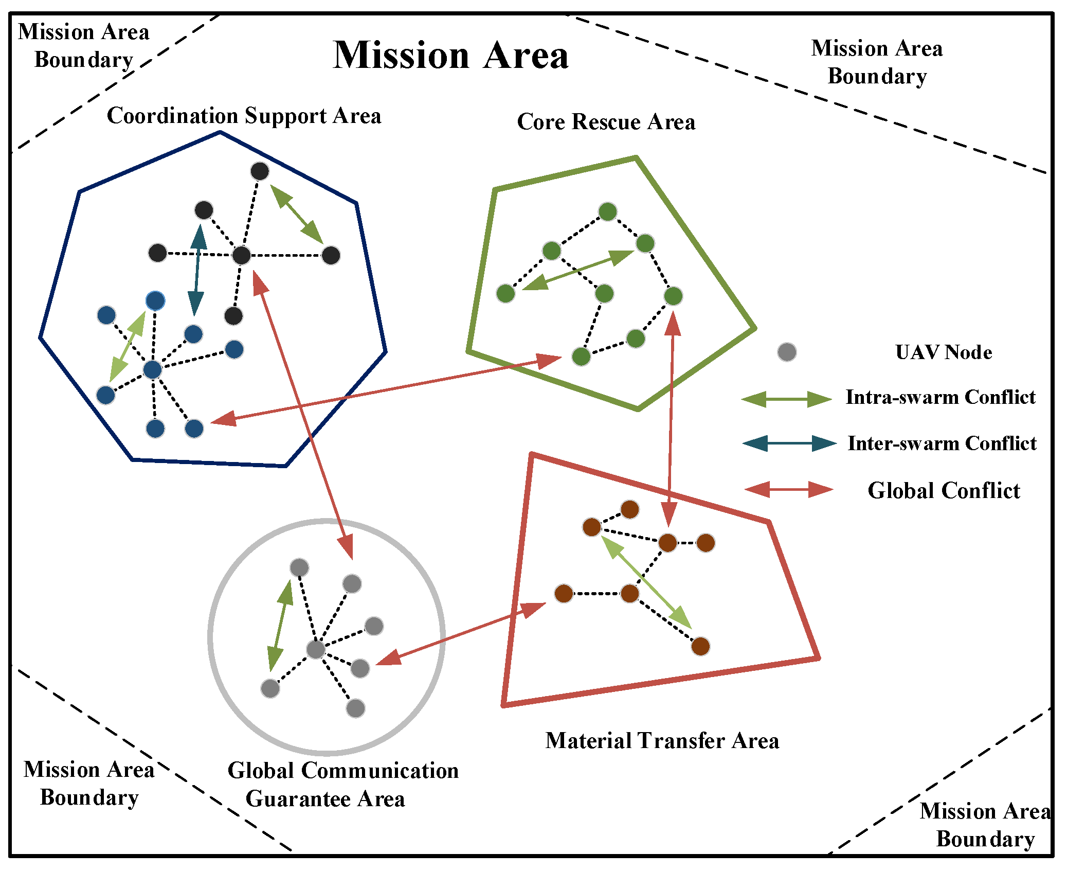
Figure 2.
Spatial-Functional two-Dimension architecture.
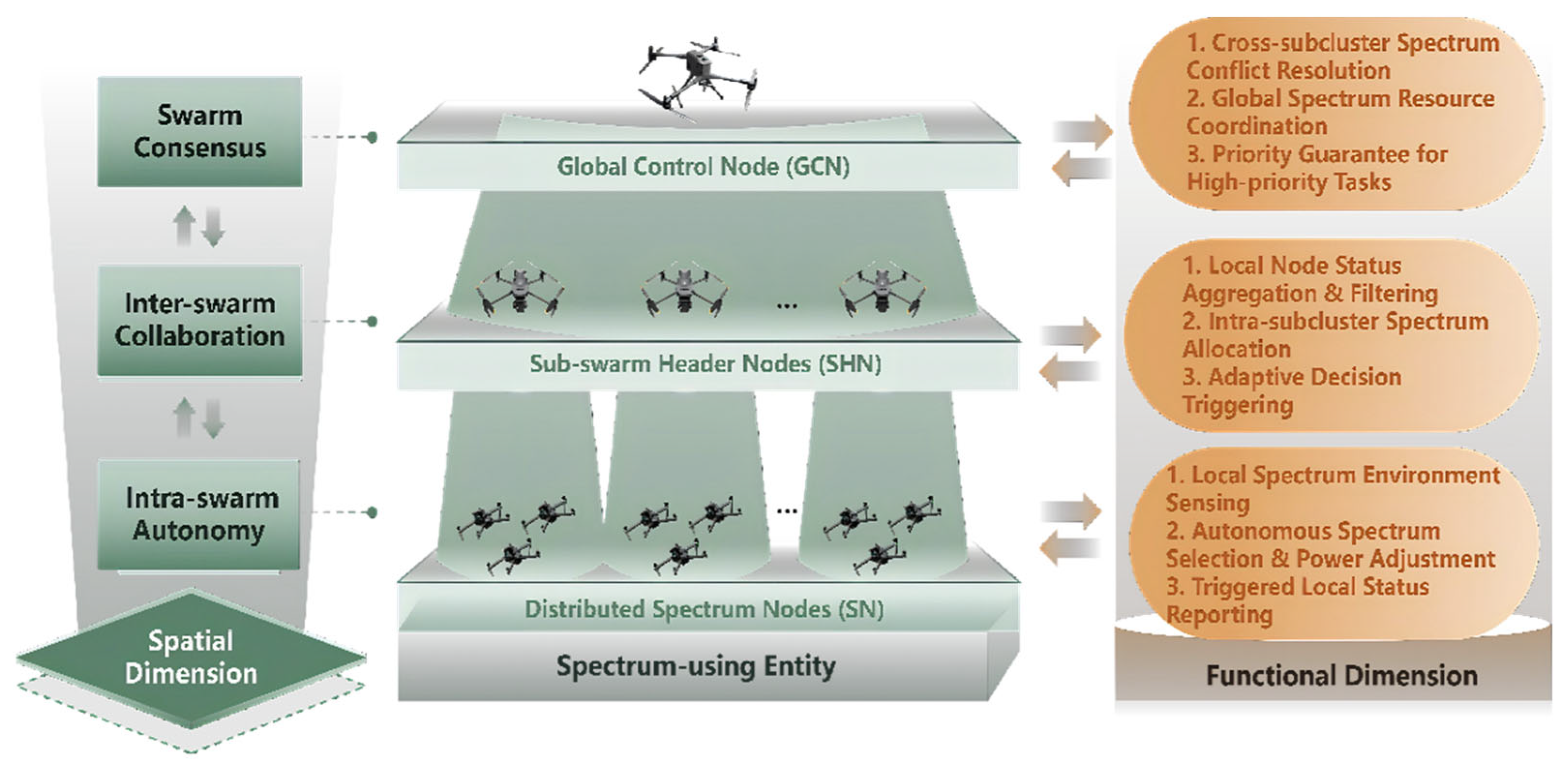
Figure 3.
Strategy selection flow of adaptive decision-making.
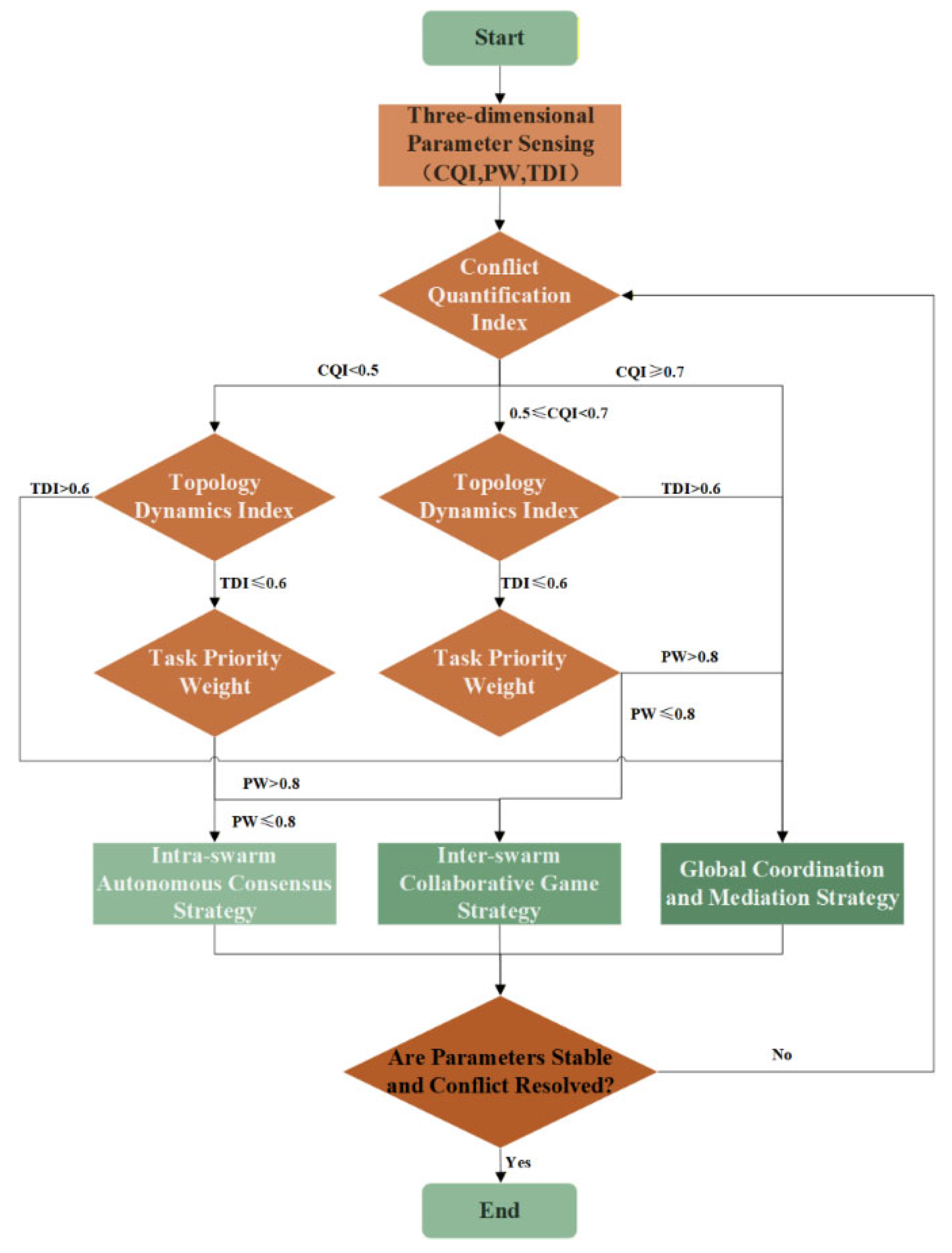
Figure 4.
RMSE convergence curves under adaptive and fixed step size schemes.
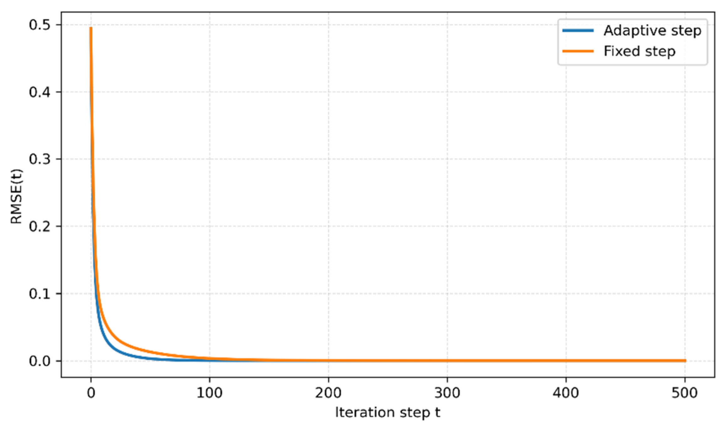
Figure 5.
Average convergence steps with different reference step sizes.
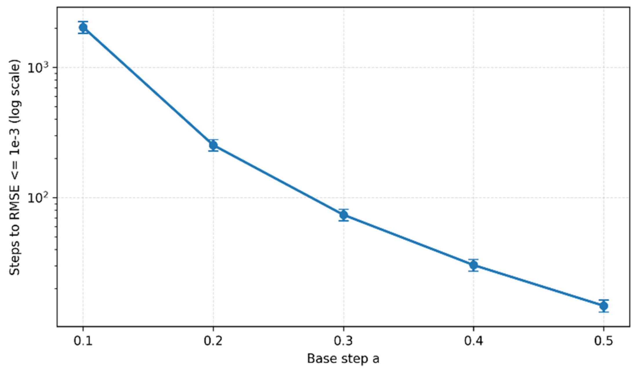
Figure 6.
RMSE attenuation trajectories with theoretical upper bound.
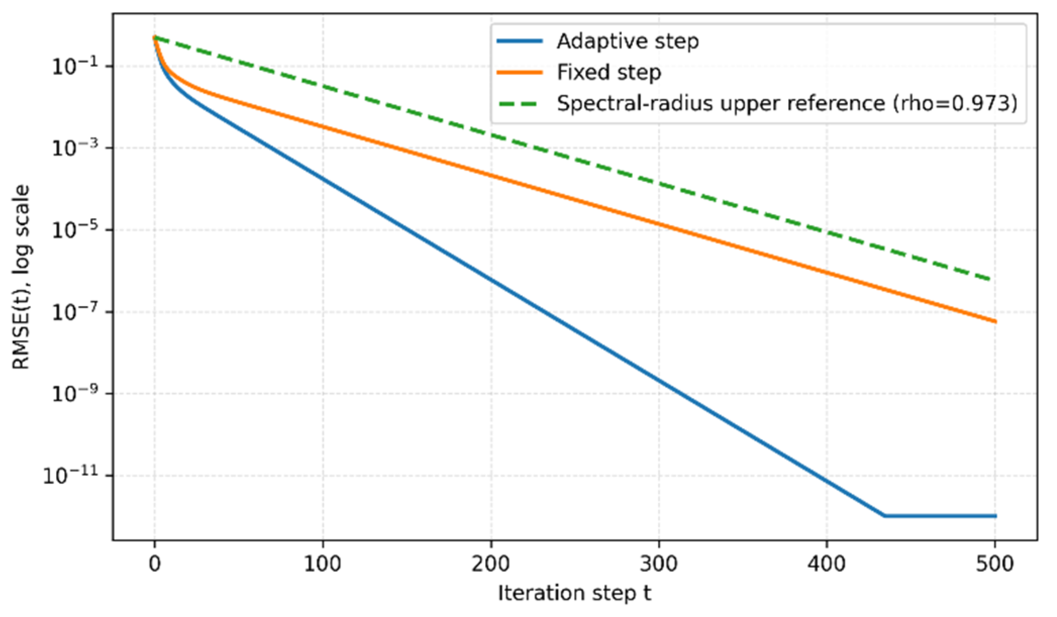
Figure 7.
RMSE response and recovery under external sudden disturbance.
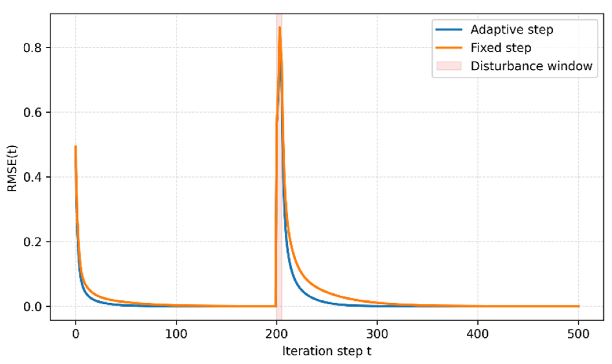
Figure 8.
RMSE recovery performance under random node failure.
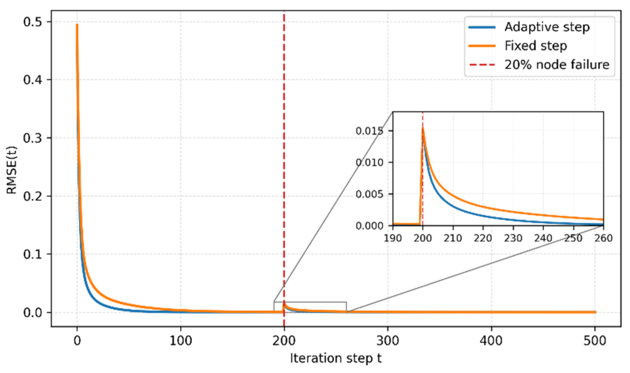
Figure 9.
Steady-state RMSE under different topology dynamics levels.
Disclaimer/Publisher’s Note: The statements, opinions and data contained in all publications are solely those of the individual author(s) and contributor(s) and not of MDPI and/or the editor(s). MDPI and/or the editor(s) disclaim responsibility for any injury to people or property resulting from any ideas, methods, instructions or products referred to in the content. |
© 2026 by the authors. Licensee MDPI, Basel, Switzerland. This article is an open access article distributed under the terms and conditions of the Creative Commons Attribution (CC BY) license.
Copyright: This open access article is published under a Creative Commons CC BY 4.0 license, which permit the free download, distribution, and reuse, provided that the author and preprint are cited in any reuse.


