

Submitted:
10 July 2026
Posted:
13 July 2026
You are already at the latest version
Abstract
Background: Researchers dealing with software engineering often express some concern about the lack of a core theory for this discipline. In fact, even the most basic concepts of software engineering—like the organization of software development life cycles—are usually described informally, with no reference to an underlying theory. Methods: In this paper, a well-known model for requirements and specifications is used as a basis for a rigorous and uniform description of software development activities. Results: The proposed approach proved suitable to describe the most popular software life cycles, as well as to describe the properties of software development activities. The proposed approach was also used to describe the properties of the software product in a way that is precise enough to support the definition of metrics. Conclusions: The proposed approach seems suitable for describing most software engineering issues and reasoning about them.
Keywords:
software development methods
; waterfall model
; software prototyping
; agile software development
; software development techniques
; software properties and metrics
1. Introduction
When software life cycle models were first proposed, they had the great merit of contributing to the systematic organization of software development. However, the proposed models [1] were no more than “boxes-and-arrows” diagrams, whose meaning were explained only in terms of the experience that brought to the definition of such life cycles and phases. So, on the one hand one could feel quite relieved to know that someone had devised methods to organize software development, an activity that could otherwise very easily turn into a rather cumbersome process; on the other hand, one was a bit disappointed by the lack of theoretical foundations.
The rather naive approach to modeling and organizing the software development process was probably justified in the seventies; unfortunately, if you look into a modern software engineering textbook, you still find boxes-and-arrows diagrams [2]. More precisely, you find several different life cycle models, all described at the same informal level as the waterfall model was described in 1970 [1].
In this paper, a notation to describe precisely software life cycles is proposed, with the aim to make reasoning about life cycles and their characteristics easier and more rigorous.
The proposed notation is based on the formula
which was proposed by Jackson [3]. In (1), R indicates the stakeholder’s requirements, i.e., “conditions over the phenomena of the environment that we wish to make true by installing the machine” while E expresses “conditions over the phenomena of the environment that we know to be true irrespective of the properties and behaviour of the machine” [3]. S is the specification of the machine, expressed in terms of the phenomena that are shared by the environment and the machine. In practice, S is specified in terms of I/O elements: in Jackson’s terminology, phenomena controlled by the environment and visible to the machine—i.e., inputs—and phenomena controlled by the machine and visible to the environment—i.e., outputs.
So, formula (1) is an entailment that reads: if the environment in which the machine is located behaves as specified in E and the machine behaves as specified in S, then the requirements described in R are satisfied. The logical entailment A ⊢ B states that from assuming A we can prove B; hence, entailment is often called provability.
It is important to note that the level of formality of formula (1) can vary. In fact, the formality of the formula depends on the formality of the descriptions E, S and R. It is possible to provide informal, text based descriptions, as well as completely formal specifications, depending on the intended use of these descriptions. If E, R and S are described formally, it is possible to prove that the truth of R descends from the truth of E and S, while informal descriptions allow only for argumentations that the truth of R descends from the truth of E and S.
According to the ISO/IEC 12207 standard [4], a life cycle is the evolution of a system, product, service, project or other human-made entity from conception through retirement; a life cycle model is a framework of processes and activities concerned with the life cycle that may be organized into stages, which also acts as a common reference for communication and understanding.
Many different software life cycle models were proposed [5], including several models that implement agile processes. Life cycle models indicate what processes and activities are carried out through the life cycle—hence, what roles and resources are used—and what relations exist among processes and activities, in terms of coordination (precedence, parallelism, …) and shared artifacts. In general, life cycle models are quite abstract: they describe processes and activities like black boxes: it is specified what is done and what artifacts are used and produced; for the sake of generalizability, life cycle models do not prescribe how (i.e., with what methods, techniques and tools) activities are carried out.
According to [4], life cycle model are useful for communication and understanding. Actually, they are useful for many purposes. From the management point of view, life cycle models provide a framework for estimating development cost and duration, for control (thanks to the possibility of associating milestones to the completion of stages, the release of artifacts, etc.), for staffing (according to the roles required by life cycle activities), etc. From the technical point of view, life cycle models provide a framework for technical decisions, like choosing the techniques and tools to be used in specific activities, or the languages and notations to be used for describing artifacts that are shared among multiple activities. Life cycle models also provide a model for reasoning on the organization of software development and the optimization of the development process.
Several life cycle models were proposed, both to improve software development and to cope with the needs of different software projects, which can call for different life cycle stages, differently organized and differently scheduled and coordinated. Unfortunately, life cycle models are still described (and taught) via boxes-and-arrows diagrams, whose semantics is generally not well defined.
In this paper, we explore the possibility of using formula (1)—and similar entailments concerning various software artifacts—as the theoretical basis for the precise definition of software life cycles. As software life cycles can be considered the basis for software engineering, the ability to describe them precisely—even formally, if required—by means of a single simple formula looks like a necessary condition for a “core theory” of software engineering.
Besides modeling life cycles, the proposed approach applies to multiple aspects of software engineering, as demonstrated throughout the paper. Among these are i) reasoning about life cycles’ activities, ii) reasoning about software artifacts and their characteristics, iii) supporting software project management activities, iv) describing software properties and defining measures.
The paper is organized as follows. Section 2 discusses previous work concerning software life cycle modeling. Section 3 provides some additional remarks concerning the basic entailment (E, S ⊢ R) used throughout the paper. Section 4 shows how formula (1) can be used to model the waterfall life cycle, while the following Section 5, Section 6 and Section 7 shows how the formula can be used to model other popular life cycles, namely the prototype, incremental and agile processes. Section 8 illustrates, via examples, the expressive power of the proposed notation and its ability to support reasoning about software artifacts and their characteristics. Section 9 shows that the proposed notation can be used also to deal with management issues. Section 10 shows how to detail the description of individual software development activities. Section 11 describes the properties of the software product in a way that is precise enough to support the definition of metrics. Finally, Section 12 draws some conclusions.
2. Background and Related Work
In most software engineering books, the waterfall life cycle is represented via a “boxes and arrows” notation, as in Figure 1 (sometimes without the backwards arrows).
The explanations of the development phases are not very precise either. For instance, Requirements analysis and definition can be described saying that “The system’s services, constraints, and goals are established by consultation with system users. They are then defined in detail and serve as a system specification.” [2].
Other authoritative sources, such as the ISO standard concerning software life cycle processes [4] or the Guide to the Software Engineering Body of Knowledge [6], provide similar definitions.
Although software engineering concepts and practices are still generally described informally and without the help of an underlying theory, some awareness of the need for software theories seems to exist. For instance, Johnson et al. expressed some concern about the lack of a core theory for software engineering [7]. They suggest that many theories exist, but none proved to be comprehensive or sound or effective enough to win the consensus of the whole software engineering community.
SEMAT (Software Engineering Methods and Theory) started an ambitious initiative for a general theory of software engineering. It resulted in the definition of the “SEMAT kernel of essential elements that are universal to all software development efforts, and a simple language to describing methods and practices.” [8]. However, the SEMAT kernel does not seem to support the type of reasoning illustrated in this paper.
Hall and Rapanotti suggested that a simple elegant formula can possibly relate the most important concepts in software engineering [9].
In this paper, a well-known model for requirements and specifications is used as a basis for rigorously and uniformly describing software development activities, and for supporting reasoning about most software engineering issues.
3. More on Formula E, S ⊢ R
With respect to [3], it is worth noting that to obtain the desired effects R, part of the environment E has to interact with the machine S: for instance, someone (or something) has to feed input data to the machine, and someone (or something) has to use the outputs. To this end, formula (1) can be rewritten as
where EI is the part of the environment that is given and that we cannot change (at least, not as part of software development activities), while ED indicates the part of the environment whose behavior can be designed to comply with our objectives. For instance, EI could be laws, business rules, the market, corporate policies, etc. ED could be the behavior of the personnel who has to interact with the machine: they can be instructed to operate in a suitable way. By distinguishing EI from ED, we make explicit that both ED and S contribute to solving the problem of achieving R in E.
Descriptions EI, ED, S and R can be classified—coherently with the view suggested by Jackson [3,10]—as follows:
- The description of EI is indicative: its properties are given and cannot be changed.
- The description of R is optative: it represents the users’ goals, which can be negotiated and possibly changed: the constraint is that the final formulation of R represents a satisfactory solution of users’ problems.
- The descriptions of ED and S are designed. We can decide the behaviour of the machine and of the part of environment we control.
As an example, consider an organization who wants to get a daily report on the value of its investments. EI describes precisely (possibly formally) the nature and composition of the investments, and the part of the environment that is relevant for the problem (e.g., the stock exchange, real estate market, etc.). R describes precisely (possibly formally) the desired report and the relationships between the reported values and the actual value of the investments in the environment.
For simplicity, in the rest of the paper, formula (1) is used instead of formula (2), intending that E = EI ∪ ED.
To show that formula (1) can be used to define precisely the most fundamental concepts of software engineering, in this paper a few among the most popular software life cycles and related development activities are modeled.
In this paper, we do not go into details about how to write E, R and S and how to show that E, S ⊢ R. The interested reader can find guidelines and examples in the literature [11] .
4. Waterfall Life Cycle
A widely acknowledged merit of the waterfall model [1,12] is that it highlights the phases of development and the artifacts that are produced within each phase. Accordingly, we expect that formula (1) can be used to precisely describe phases and artifacts, as well as the relationships that link phases and artifacts.
The waterfall life cycle has many shortcomings [13]; this paper does not intend to endorse this life cycle, but only to show that it can be properly described by means of formula (1) and related entailments.
4.1. Requirements Analysis and Specification
In (1) R is the artifact that specifies users’ requirements and E is the artifact that describes the properties of the part of the environment that is relevant to the problem: having specified E and R, we are in a situation that could be described as
In (3) the presence of the question mark makes explicit that this is a problem statement: we have an environment that behaves (according to its own rules) unsatisfactorily, we have some desires, and we are looking for a way to make the environment behave as desired.
4.2. Solution Specification and Requirements Validation
Up to a few decades ago—programmable computers not being available—the only possible way to satisfy user requirements was to instruct some part of the environment to behave in a way that led to satisfying requirements; this situation can be model as
For instance, if R involved collecting news in the first half of the eighteenth century, ED would likely involve couriers and horses.
Today, we look for a machine specification S such that E, S ⊢ R. Being able to specify S is important for at least two reasons:
- 1.
- If we can build a convincing argument that E, S ⊢ R, then we have verified that R can actually be satisfied. In fact, it may happen that formula (3) has no solution at all: in such a case, requirements R have to be modified.
- 2.
- The specification S is the input for the design phase.
It is important to note that S is not unique. In general, formula (3) can be satisfied by multiple machine specifications: E, S1 ⊢ R; E, S2⊢ R; ...; E, Sn⊢ R. Examples can be found in [14]. Accordingly, the specification phase involves identifying and assessing multiple machine specifications, and possibly helping the stakeholders choosing which specification should be implemented.
4.3. Implementation (Design and Coding) Phases
Specifications S are the input to the design and coding phases, whose expected output is a machine that implements S. Usually the machine is not built from scratch, because it would be exceedingly expensive and it would take a very long time; instead, a given programmable HW/SW platform M is “configured” by means of a program P in order to behave as specified in S . For instance, M could be a Linux machine equipped with suitable software (e.g., JavaScipt, MySQL, etc.): the developers’ task is to build a program that runs on the given platform according to the given specifications. Note that in general P has to be built, while M can be chosen among several available alternatives: for instance, one could use one of the many virtual machines available in the cloud.
The relationship that links P and S is quite similar to the relationship that links S and R: we can write
meaning that the platform M running program P behaves as specified in S.
It must be stressed that S is defined in terms of the “phenomena” that are shared by the world (modeled by E) and the machine (M & P) . In practical terms, S is a description of the machine in terms of I/O.
4.4. Verification
The purpose of verification is to show that the proposed implementation actually satisfies the specifications, i.e., that (4) holds.
In principle, the verification can be a formal proof, based on the formal descriptions of M, P and S. However, this it is generally impractical, because a formal and accurate description of both M and P would be needed, and writing such descriptions is very difficult and expensive. In fact, formal proofs are usually carried out only on small fragments of S that are considered very critical, hence worth the effort of deriving formal proofs.
Usually, verification is performed by means of testing, i.e., running the program and checking that it behaves as specified. The following discussion makes reference to verification via testing.
Before proceeding, we need to notice that E, S and R are descriptions [15]. During testing, we use the real platform MR and the actual program PR. So, ideally the goal of verification is to show that
Formula (5) states that the combination of MR and PR behaves in a way that conforms to the specifications under all possible circumstances that may occur in the environment. In fact, description S is expressed in terms of all the phenomena that are shared by the machine and the environment. Since experimentally proving the truth of entailment (5) under all possible circumstances is generally not possible, the actual testing activity consists in checking that
where SR is expressed in terms of the relatively small set of phenomena occurring during testing (i.e., the set of inputs supplied to the machine and the set of corresponding outputs). These phenomena can be originated in the real environment or can be simulated in the testing laboratory. In both cases, the set of testing phenomena can be considered as originated by an environment ET, whose phenomena and behaviours are subsets of E’s.
Since MR and PR are exercised in a subset of the conditions and situations that may occur in the real world, the proved behavior SR is usually only a subset of the specified behavior S (that is, SR ⊆ S). In general, verification is considered successful if (6) holds and the difference S – SR includes only situations that are considered hardly relevant or “essentially equivalent” to situations in SR. In such conditions, it is assumed that if (6) holds, then (5) holds as well.
4.5. Validation
When considering the validation of the proposed solution, we have to verify that the proposed implementation satisfies user requirements, i.e.,
Note that specifications S do not appear in formula (7). In fact, specification S are just an artifact of the software development process: since proceeding directly from the problem statement (3) to the solution described in (7) is generally exceedingly complex and difficult, specifications S were introduced to make the development process a viable step-by-step activity.
Ideally, validation should prove that
where ER represents the real environment, and RR describes the real needs of the users.
During development, it is customary to assume that R=RR, i.e., that the documented requirements match the actual user requirements, and E=ER, that is, the description of the environment is an accurate and effective representation of the actual environment. Unfortunately, both assumptions may be false, in practice: in such cases the implemented system can fail to cope with unexpected (hence, undocumented) environmental conditions and/or fails to satisfy the actual user needs (which have not been expressed or properly understood).
Since also validation is typically done via testing, the huge number of relevant phenomena in the real world makes it generally impossible to experimentally prove (8). Therefore, in practice validation shows that
where EVT ⊂ ER is the subset of the environment actually used in the tests and RO is the description of the observed effects in the environment caused by MR and PR. EVT is generally different from ET, i.e., the achievement of requirements is tested via a different set of test cases with respect to the one used to verify the achievement of specifications.
If RO is acceptable or not depends on the specific situation. In a user acceptance test (UAT) aiming to verify if the system behaves as described in a contract, we need that RO ⊆ R, where R describes the behaviour as defined in the contract.
If the “real” requirements RR are verified, verification succeeds if RO ⊂ RR. In what follows we assume this situation.
4.6. Representing the Waterfall life Cycle
Using the formulae introduced above, it is possible to rewrite the representation of the waterfall life cycle as shown in Figure 2. For each stage, the delivered artifacts are specified, together with the relationships that should hold: specifying such relationships contributes to clarify the meaning and intended usage of artifacts.
In Figure 2, activities are described as black boxes, in which the work to be done depends on what is available at the beginning of the activity and what has to be achieved. For instance, before Design&coding we have specifications S that satisfy R in E, and we are looking for a machine (i.e., a computing platform M equipped with a program P) that satisfies S. Hence, the purpose of the Design&coding phase is to (somehow) define M and P such that M, P ⊢ S. The proposed approach can be used also to describe development processes at finer granularity levels: an example showing how to describe some details of Design&coding is given in Section 10.
The relationships among artifacts defined in the model also explain the presence of loops. Consider for instance the feedback from Specification to Requirements analysis: it occurs when it is not possible to define S such that E, S ⊢ R. The cause may be that requirements R are too challenging, or the description of E is wrong or incomplete. Similarly, the loop from Design&coding to Specification occurs when it is not possible to achieve M, P ⊢ S, i.e., we are not able to build a program P that, executed on a machine M, satisfies the specifications. In such a case, specifications must be modified (i.e., a different way to satisfy R must be defined), or the requirements R themselves must be modified (usually going back to Requirements analysis and looking for a less ambitious but still satisfactory definition R).
Descriptions in Figure 2 could also be made more formal: for instance, you backtrack from Specifications to Requirements analysis when S: E, S ⊢ R ∧ viable(S), where viable(S) means that S appears to be implementable at reasonable costs and in reasonable time.
Note that in general SR ⊆ S is considered representative of S, i.e., having proved that SR is true makes us confident that also S is true. Similarly, having proved that RO is satisfied makes us confident that also RR is satisfied.
4.7. Development Activities as Learning Processes
In Figure 2, development activities are described as black boxes, having some properties that hold at the beginning of the activity, and aiming to satisfy some property that has to hold at the end of the activity.
It has been observed that the steps carried out within a development activity involve exploration, learning, interaction with the world and with the stakeholders. Those operations are guided by the evaluation of contingencies, the identification of options, and decision-making. Modeling these activities is important, because the learning process, in which knowledge is collected and refined, is at the core of software development.
Considering the specification phase as an example, let us analyze the role of learning in moving from a situation when S does not exist to the delivery of satisfactory S: S describes the data flow between the environment and the machine, and managing such data flow (i.e., supplying the input data and consuming the output) involves some operating costs; therefore, the definition of S delivered by the specification activity should satisfy the condition that the operating costs of S are acceptable. This involves the definition of the “operating cost” property of S, and of lower-level attributes of S (such as the size and frequency of inputs, or the complexity of outputs), upon which the operating costs are defined. All this requires talking with the user (who knows the threshold below which operating costs are fair) and analyzing details of S (i.e., of the interaction between the environment and the HW/SW machine). The very notion of operating costs could be the result of a learning process during which the point of view of the user is explored and the properties of S related to operating costs are identified.
In the subsequent design and coding phase, it could happen that no implementation can be found, whose development costs are reasonable. This causes backtracking to the specification phase, where alternative definitions of S are sought. It is possible that some knowledge is provided by developers concerning costs of implementing specifications, so that when looking for alternative specifications, the analysts can exclude the most expensive candidates. In this case we have some knowledge that flows back from a development stage to the preceding one.
This learning process can be described à la Jackson: e.g., at the end of the specification phase E, S ⊢ R ∧ operatingCost(S) < K; similarly, the end of the design and coding phase, E, M, P ⊢ S ∧ viable(P), where developmentCost(P) ≤ C ⇒ viable(P).
5. Prototype Life Cycle
There are several possible reasons to build a prototype. Here we assume that the prototype is used to clarify requirements, by getting early feedback from the users that lets developers better understand their needs. Initially, requirements are uncertain, that is, we have written R, but the “real requirements” RR could be different. In practice, we are addressing problem E, ? ⊢ R while we should address E, ? ⊢ RR. In this—quite common—situation, we risk to build a machine S that yields E, S ⊢ R ≠ RR, so that the real user’s requirements RR are not fully satisfied.
To clarify the requirements, the prototype life cycle prescribes that we build a prototype program PP that runs on platform M and implements SS, a subset of specifications S. The reason why the prototype usually implements only a subset of the specifications is that it must be available in short time and at little cost, and it needs to concentrate only on RS, the subset of R that contains the uncertain requirements to be clarified. Therefore, prototype PP aims to implement only part of the machine features (SS ⊂ S) and satisfy only part of the user requirements (RS ⊂ R):
When the prototype is run, it is shown that
where RPP is the actual (visible) effect of the execution of the prototype in the environment. RPP is assessed by the user: based on this assessment, requirements are possibly revised, i.e., the problem is reformulated as E, ? ⊢ R’. When writing the new version of requirements R’:
- a)
- The part of RPP that has been approved by the user and was already in R is retained.
- b)
- The part of RPP that has been approved by the user and was not in R is added.
- c)
- The part of RPP that was in R but has been disapproved by the user is suitably changed. In fact, a strong point of the prototype life cycle is that usually the user does not just reject parts of RPP: instead he/she provides indications on how to change the system’s behavior to make it acceptable.
- d)
- The user may also identify missing requirements, i.e., requirements that are neither in RPP nor in R: these are added.
Concerning point c), part of the knowledge concerning RPP usually applies also to parts of R not included in RPP. For instance, if the user approved the visualization of data and information as implemented in PPR, then the same type and style of visualization is likely to be usable in the rest of the system. In any case, the user can be explicitly asked questions on issues raised by the approval or rejection of RPP features.
If we are not confident with the new formulation of requirements R’, we can build a second prototype PP2R, execute it (E, MR, PP2R ⊢ RPP2), evaluate RPP2 and so on.
When we are confident that the specification of requirements is correct, we can either throw away the prototype and restart the implementation from scratch, or build on the prototype. In the latter case, the program will incorporate the final prototype PPR, so that
where P is the part of the program that is added to the prototype to complete the implementation, and R’ is the description of requirements based on the clarifications yielded by the prototypes.
6. Iterative Incremental Development
Iterative development life cycles are organized into iterations, each one aiming at implementing a new chunk of requirements. To this end, it must be possible to partition requirements into pieces, as follows:
Note that Ri ∩ Rj being empty is not always guaranteed.
The first iteration addresses R1:
P1 is tested as described in the waterfall section: the only difference being that here P1 is tested against S1 and R1, not against the whole specifications and requirements, as in the waterfall life cycle. In what follows the description of testing is skipped for the sake of simplicity.
The following iterations are typically aimed at:
- a)
- Satisfying more requirements;
- b)
- Correcting defects found in previous implementations;
- c)
- Taking into considerations changes of already implemented requirements.
If there are no changes in requirements and no defects to correct, the work done in the second iteration is described by the following pair of formulae:
Note that during the first iteration it is possible that R2 is changed (e.g., because the user changed his/her mind). In such case, changing R2 does not imply changing any other artifacts. It is also possible that R2 was not entirely known earlier, and its description is completed just before the beginning of the second one.
Concerning E, M, P1 ∪ P2⊢ S1∪ S2, in some cases it could be necessary to change P1 to make it communicate properly with P2. However, a careful choice of the architecture of P1 should make it possible to add P2 without changing P1.
If there are defects to correct, and no changes in requirements, the specifications are unchanged and the implementation work is described by the following formula:
where P1’ is the corrected version of P1.
If there are changes in already implemented requirements (i.e., R1 was replaced by R1’) and no defects to correct, we may be lucky and discover that P1 satisfies R1’; however, in general the work done in the second iteration involves redefining S1 and correcting P1, as described by the following pair of formulae:
If there are both changes in already implemented requirements (i.e., R1 was replaced by R1’) and defects to correct, the work done in the second iteration is still described by the pair of formulae (14). This stresses the fact that the work carried out in an iteration is useful to both correct defects and address changes in requirements.
The remaining iterations can be described along the same line as the second one.
7. Definitions of Agile Processes and Related Techniques
Researchers and practitioners started proposing agile development methods in the 90’s. In 2001 the Agile Manifesto was published, stating the values and principles of agile processes [16]. Since then, agile processes increasingly gained consensus: today they are very popular and widely practiced [17].
There are several proposals that can be classified as agile techniques (e.g., Scrum, Extreme Programming, Feature Driven Development, etc.). Because of space reasons we cannot discuss them all in this paper: in this section, a few selected “typical” aspects of agile processes are modeled. It is expected that these selected aspects are representative of most agile process features, so that being able to successfully cope with them makes the readers confident that the proposed approach is generally applicable in the context of agile process.
Agile processes are generally characterized by the prioritization of requirements. That is, requirements are partitioned into pieces and arranged in order of priority. For instance, in Scrum [18] each sprint addresses the piece of backlog that brings the greatest value for the user. If we call Ri the piece of requirements addressed by the ith sprint, we have that
After the ith sprint, , where P is the program obtained through the first i sprints.
The iterative incremental development works as described in Section 6. However, a few practices that are typical of agile processes need to be precisely defined, as discussed below.
7.1. Refactoring
Refactoring involves changing the implementation of a given specification to improve its structural qualities, while preserving its functionality: the new code has to implement exactly the same specification as the original code. So, before refactoring we have
After refactoring:
where PI is the improved code obtained via refactoring: it implements the same specifications S as P, and passes the same tests (see Section 4.4) as P.
It should be possible to prove that some measures (e.g., those dealing with code complexity, cohesion, coupling, etc.) are better for PI than for P.
7.2. Dealing with Changes
A most relevant characteristic of agile processes is their ability to cope with change. Changes can be:
- 1.
- In the environment E.
- 2.
- In the user requirements R (e.g., the user “changes his/her mind”).
- 3.
- In the specification S, i.e., in the way requirements R will be satisfied.
- 4.
- In the way S is implemented, that is, in P, assuming that the hardware/software platform M is not changed.
- 5.
- In the platform M.
In cases 1 and 2, it could be the developers’ understanding of E or R to change: the effect in practice is the same as E or R actually changed. Of course, several of the above changes may occur at the same time: here we consider only one type of change at a time, for clarity.
Case 1 E changes into E’. This may also require that R changes into R’. In any case, S has generally to be changed as well, leading to E’, S’ ⊢ R’. Consequently, the code is updated to implement S’: M, P’ ⊢ S’.
Case 2 R changes into R’. This implies that the specifications are revised to accommodate for the new requirements: E, S’ ⊢ R’; consequently, the code is updated to implement S’: M, P’ ⊢ S’. Exceptionally, it may happen that E, S ⊢ R’, that is, the original specifications satisfy also the new requirements; thus, nothing has to be changed, except the description of requirements.
Case 3: E, S ⊢ R is changed into E, S’ ⊢ R. Accordingly, a new program P’ is needed to satisfy S’: M, P’ ⊢ S’. Note: this is one of the points where agile processes are most different from traditional processes. In fact, traditional “design for change” techniques could sometimes ease the transition from P to P’. Agile processes, which predicate the simplicity in design and the YAGNI (you aren’t gonna need it) principle, will possibly require non trivial changes of P to get P’.
Case 4: E, S ⊢ R is unchanged. We need a new P’ that satisfies M, P’ ⊢ S. P’ may be needed because some quality of P is not acceptable: quite often, P is changed to make it easier to extend in the following sprints.
Case 5: Usually, platform M is not controlled by the software developers who have to satisfy R. Hopefully, the changes in M are “backward compatible” so that there is no need to change P as a consequence of changes of M; that is, M, P ⊢ S implies M’, P ⊢ S. However, it may be the case that some change is required, i.e., M’, P’ ⊢ S.
7.3. Test Driven Development
Test driven development (TDD) is a technique that—though not exclusive of agile processes—is an essential component of many agile development processes. TDD assumes that unit-level test cases are written first, then the code that passes the test is written. Therefore, we first need to introduce the concept of unit (alias module).
To organize the system into modules, both specifications and requirements are decomposed into pieces: and . Hence,
Ideally, each module Pi implements a fraction of the specifications:
The implementation of the whole system involves that
In the context of agile processes, the specification of a module is usually very informal and often rather imprecise. We can represent this situation (maybe a bit radically) as E, ? ⊢ Ri. However,
- 1)
- Building the program making reference to the requirements is exceedingly complex and error prone (in fact, this is why specifications are introduced in the classical waterfall life cycle).
- 2)
- In any case, the program has to be tested, to verify if it complies with the given requirements. To this end, we have to design a set of test cases that exercise the program in a representative set of conditions for all requirements (as discussed in Section 4.4).
The novelty of test-driven development is that test cases are designed before implementation, rather than afterwards. So, test cases guide the development instead of specifications. In other words, the goal of implementation is not implementing a program that satisfies the given specifications; instead, it is implementing a program that passes the tests: a program that passes the tests is assumed to satisfy requirements. Clearly, the test cases have to be carefully devised, so as to properly exercise the requirements.
All this can be modeled by means of the proposed method as follows. Given the requirements Ri to be satisfied, tests are designed first. Designing tests involves identifying a subset of the environment in which the program will be executed. This subset of the environment, named EVT, includes phenomena that cause the machine PToBe (still to be implemented) to react, thus causing the expected effects Ri’. As EVT is a subset of E, Ri’ is a subset of Ri:
A condition for effective testing is that showing that EVT, MR, P ⊢ Ri’ holds is sufficient evidence that EVT, MR, P ⊢ Ri holds as well.
An important quality of test-driven development—possibly the very reason for adopting it—is that programmers are in charge of writing the test cases at the unit level. To define test cases—i.e., to identify EVT and the corresponding outcome Ri’—programmers have to gain a good understanding of requirements, while this is not required in the waterfall life cycle, where specifications somehow hide requirements from programmers.
The presence of PToBe in formula (16) stresses that tests are defined when it has not yet been devised how requirements will be satisfied. After having defined the tests, code Pi is implemented and tested:
where RiR represent the actual observed effects of the executions in the environment. If RiR – Ri’ , (i.e., if Pi causes some undesired effects) Pi is modified; this process is iterated (in the following sprints) until RiR = Ri’.
In this way, specifications may remain unspoken, but—since they are the set of phenomena and relations that in conjunction with E entail Ri—they are implicitly defined via test cases.
7.4. More on Refactoring
Refactoring is started when we have a program that satisfies tests (as described in the previous section) but does not satisfy other needs. In the context of agile processes, it is often the case that it is hard to integrate new features in the program.
The typical situation is when the ith iteration is complete, hence M, Pj⊢ Sj, but it is difficult to write Pi+1 so that M, Pj∪ Pi+1 ⊢ Sj∪ Si+1.
So, the goal of refactoring is to write PR that can substitute Pj so that
- 1)
- M, PR ⊢ Sj, and
- 2)
- Building Pi+1 so that M, PR ∪ Pi+1⊢ Sj∪ Si+1 is relatively easy.
Note that in general creating PR does not require changing all the modules. If the system is properly architected, changing just a few module is sufficient.
PR is approved if
An important point is that often PR is obtained by means of a sequence of small changes. Therefore, it is possible to run the tests—as in (4)—as soon as any small change has been implemented, so that the refactoring process is continuously under control.
8. Explanatory Power of the Proposed Approach
The expressive power of the proposed notation and its ability to support reasoning about software artifacts and their characteristics is illustrated in the following sections, via a set of examples.
8.1. Verification vs. Validation
If we look for definitions of software verification and validation activities, it is very likely that we find the following ones [19]:
- Validation: Are we building the right product?
- Verification: Are we building the product right?
The definition of validation suggests that the product must be right from the point of view of the user, while the definition of the verification suggests that it is the building of the project that must be right, i.e., it must be correct from a technical point of view.
Although these definitions convey a general idea of the meaning of verification and validation, they are by no means precise.
Consider the definitions using Jackson’s formulae:
- Verification deals with proving that MR, PR ⊢ S
- Validation deals with proving that ER, MR, PR ⊢ R
Not only the latter formulation is more precise than traditional definitions, but it supports better reasoning about the considered activities. For instance, our formulae highlight the difference between descriptions (like E and S) and the actual artifacts (like ER and SR). In fact, “Are we building the right product?” could refer to R—the description of the user requirements as they were understood and documented, and possibly reported in the contract—or to RR—the actual requirements, i.e., what users have in mind.
Proving ER, MR, PR ⊢ R may be inconclusive, when R is imprecise or incomplete. The proof can be sufficient to demonstrate that contract obligations have been satisfied, but it does not imply that the user is actually satisfied with the delivered product.
Finally, we can observe that our notation supports reasoning about how to carry out verification and validation via testing, as discussed in Section 4.4 and Section 4.5 above.
8.2. The “What” and the “How”
A very popular way of describing software specifications is that they indicate what has to be developed, as opposed to design, which concerns how the software is built. This is correct only in the machine domain. Specifications S indicate the behavior of the machine in terms of interactions with the world: how S is satisfied depends on P and M.
However, let us look at formula E, S ⊢ R, which does not involve the implementation, as it represents the point of view of the stakeholders, domain experts, users, customers, etc. To these people, S specifies how requirements are satisfied. In fact, S is the solution of the problem expressed as E, ? ⊢ R.
8.3. Explaining the Difference Between Proofs and Actual Behaviour
Donald Knuth’s famous statement “Beware of bugs in the above code; I have only proved it correct, not tried it” [20] can be explained in terms of (1), (4), (7) and their real world counterparts.
Knuth’s statement has multiple meanings.
A first meaning is that Knuth proved M, P ⊢ S, but not E, S ⊢ R. In other words, the code implements correctly a given specification, but this does not guarantee that when we use the program in the environment, it will satisfy the user’s needs. Quite interestingly, this situation may lead to the recurring situation when the user blames the programmer (“your program does not work!”) and the programmer blames the user (“you are not using my program as it was supposed to be used!”).
A second possibility is that Knuth proved E, M, P ⊢ R, but the description of the word E fails to represent the actual behavior of the word ER (it could be incomplete, incorrect, not enough detailed, etc.). Consequently, ER, M, P ⊢ R may not hold. This is the case of the famous Ariane 5 disaster [21]: E4, M, P ⊢ R (where E4 describes the Ariane 4 environment) held, so it was assumed that E5, M, P ⊢ R (where E5 describes the Ariane 5 environment) held as well. The demonstration that the latter assumption was false was quite spectacular and expensive.
Another possibility is that an ideal model of the machine M executing P was used in the proof. In practice, the machine is subject to failures or is not fast enough, or has some other problem, so that E, MR, P ⊢ R does not hold. This is the case of the famous Pentium floating point unit bug [22]: a correct program may not achieve the desired results because of failures in the real machine.
8.4. Reasoning About Software Development Organization
In the requirements analysis phase, requirements are optative, since they describe “the desired condition over the phenomena of the environment”, as stated by Jackson. However, E and R are given to the specification phase, as shown in (3): people who are responsible for writing the specifications S cannot change the requirements R: if there is a problem with defining S we have to go back to the requirements analysis phase to change R. Is this organization of work optimal? An alternative could be a single phase in which both R and S are defined in parallel or in an interleaved manner.
Similarly, in the Design&coding phase of a waterfall life cycle, R and S are to be considered indicative: people in charge of implementation cannot change the requirements or the specifications, also because they may not have a full understanding of the reasons why R and S were defined as they were. The situation can be very different in agile processes, where developers can also be in charge of maintaining requirements.
8.5. Extending the Model Scope Beyond the Software Life Cycle
In general, software development is carried out to achieve some high level business needs: the situation can be expressed via formula E, ? ⊢ N, where N describes the business needs. In principle, it is possible to devise S such that E, S ⊢ N. However, this is difficult, because we should devise a strategy for achieving N and the specification of the machine that implements such strategy in a single step. Moreover, S would be a mixed-up description of the strategy adopted to achieve N and the specification of the machine that implements the strategy.
Let us consider the following example: a retail company wants to inform potential clients about the available products, with the ultimate goal of increasing sales: this is described via N. Now, there are several ways (strategies) to satisfy need N: classical TV ads, distributing paper catalogues, notifying known clients via social apps, etc. Requirements R describe the chosen strategy (if it is decided to adopt multiple strategies concurrently, each one can be described by a document R). So, R can be seen as a solution to achieve N. The relationship between the problem and solution elements can be synthetically expressed by the following system of formulae [14]:
The system of formulae (18) shows that to satisfy the business needs N we look for both an effective strategy (i.e., we need that R satisfies N) and an effective implementation of the strategy (i.e., S satisfies R). A perfect implementation of an ineffective strategy will not achieve the needed results; of course, a defective implementation of a good strategy will fail similarly. Interestingly, it is possible—though quite unlikely—that a defective implementation of an ineffective strategy achieves the sought objectives.
It is important to observe that needs are typically expressed by people that are deeply concerned with the business, but have little knowledge about software technologies, so they are usually not able to express requirements for software: e.g., they could express requirements that are excessively hard to achieve (i.e., they could be too expensive, or could require excessively long development time) or unnecessarily constrained (i.e., the available technology and development methods make it possible to achieve much more effective and efficient solutions with approximately the same effort and cost). It is therefore essential that business analysts make a good design (!) work, by not only understanding users’ needs, but also helping end users in shaping and formulating software requirements for which viable and convenient software solutions exist.
9. Supporting Management
The proposed approach can be used to support the management of projects, as shown via a few examples.
9.1. What Should Be Defined in a Software Development Contract?
The concepts introduced in the previous sections support some considerations about software development contracts.
The object of the contract is typically the construction of a program P such that, given M and S, makes the entailment M, P ⊢ S true. Even though the user/customer is ultimately interested in R, we saw that there are many S such that E, S ⊢ R, and these S are usually characterized by different costs and performances; thus, it is reasonable that a specific S is chosen as the object of the contract.
Even though S is the main object of the contract, it is often the case that the contract mentions also several other artifacts, including the following:
- The machine M that will be “configured” by means of P is usually described in the contract. I.e., it is said on which platform the program P is expected to run.
- Some characteristics of P are often constrained. For instance, P should use an existing database or interface with an existing system.
- The environment in which the program has to contribute to the achievement of the requirements should be specified as well.
- The acceptance test of P is also generally described. This involves specifying EVT (see Section 4.5).
Having defined the development phases as described in the previous sections, it is easy to relate costs to phases or to the delivery of artifacts. The cost of code implementation is the cost of creating P such that M, P ⊢ S. The cost of code implementation may include testing, that is, defining ET and making sure that MR, PR ⊢ SR⊆ S, where SR is expressed in terms of the phenomena shared between ET ⊂ E and the machine.
9.2. Effort Estimation
A life cycle model should be useful also for supporting software development management. To illustrate how, here we consider the problem of effort estimation when the waterfall life cycle model is used.
It is reasonable to assume that the development effort depends on the artifacts to be created or used in the process; that is, we can write an equation like the following:
where m(X) indicates a set of measures of artifact X.
By reasoning on the artifacts and their nature, we could identify function f, as well as the measures needed. For instance, (1) is coherent with the intermediate version of the COCOMO model [23], which involves the size of the program being developed (a measure of P), and a set of parameters like the required reliability (a measure of R), the volatility of the machine (a measure of M), and the amount of data to be managed (a measure of E).
So, it appears possible to identify a set of artifacts and their characteristics from our life cycle model and use them to build a model of the development effort. However, having a precise definition of the life cycle lets us go beyond COCOMO. If—as is fairly usual—effort estimation is performed at the end of the specification phase and concerns the subsequent activities, the model of the waterfall life cycle given in Section 4.6 suggests that the measure of the size of P is not available at estimation time; instead, S is available for measuring. Originally, COCOMO adopted lines of code—a measure of P—as a proxy of the measure of S. The problem with this choice is that the given specifications S can be satisfied by different programs like P1 and P2 (M, P1 ⊢ S and M, P2 ⊢ S), having different sizes, i.e., m(P1) ≠ m(P2).
This problem was solved by Albrecht, who proposed a measure of S (the Function Point [24]), which does not depend on the technology used for implementing S, on the programmers and on any other characteristic of the development environment.
Going back to (19), we can thus redefine f so that it uses a measure of the size of S, instead of a measure of the size of P. Quite noticeably, COCOMO II [25] allows for using measures of the size of S.
So, our definitions can be used to explain the motivations that induced Albrecht to define a technology-independent measure of size, and to explain one of the differences between COCOMO ’82 and COCOMO II.
We can proceed further, by considering that the development effort depends also on how some activities are carried out. Let us consider verification and validation: the definitions of these activities given in Section 4.4 and Section 4.5 suggests that the cost of verification depends on the extent of ET, while the cost of validation depends on the extent of EVT. Accordingly, (19) should be rewritten as follows:
9.3. Project Monitoring
One of the most important activities of project management consists in monitoring the progress of the development process. Some monitoring activities concern the measurement of relevant properties of the software products: examples of how the proposed approach can be used in supporting product property measurement are given in Section 11.1, which deals with robustness, and in Section 11.2, which deals with usability. Here we deal with the measurement of process activities.
In our approach, activities are specified via entailments. For instance, with formula M, P ⊢ S (4) we represent the goal of the implementation phase. Implementation starts when P is not existent, i.e., M, ? ⊢ S, and ends when the goal expressed by formula (4) has been achieved. Monitoring the implementation activity involves evaluating “to what extent” formula (4) holds. In fact, at a given moment during development, we have that
where Pp is the partial implementation of P achieved when the observation is performed, and Sp is the fraction of the specifications implemented by Pp.
To measure the progress of the activity, formula (21) suggests that we have two possibilities:
- 1)
- Measuring the partial implementation Pp. In this case we can produce a measure m(Pp), where the function m to be applied to Pp depends on the technology used to implement Pp: it could be lines of code, the number of classes and methods, etc. The limit of this approach is that it provides only absolute indications, not relative ones: for instance, we may know that 10,000 LoC have been coded, but we still do not know if we are close to finish the coding or if we are just half way through the coding, since we do not know the size in LoC of the final product P.
- 2)
- Measuring the progress in terms of how much of S has been satisfied. In this case we can provide a suitable measure m(Sp); for instance, we could measure how many function points are currently implemented by Pp. We could also provide the measure of m(Sp)/m(S), which tells us what fraction of the specifications has been implemented.
Measuring m(Sp) is usually suitable for iterative and agile processes, where each iteration or sprint is expected to implement an additional “chunk” of S and R. However, in other contexts, measuring m(Sp) could provide little insight into the state of development: for instance, if development is almost complete, but a single small function used by all the others is missing, we would have m(Sp)=0, since no working functionality has been provided yet.
Other types of process measures can be devised using the same type of reasoning described above. In fact, with the proposed notation, a generic activity is described via entailment E, X ⊢ Y. At any moment before the conclusion of the activity, the situation can be described by E, Xp ⊢ Yp. So, it is generally possible to measure m(Xp), m(Yp), and m(Yp)/m(Y).
It could be observed that the specification of monitoring activities should include the indication of when the measures are carried out. To this end, we can associate time to our formulae; for instance, E, Xp(t) ⊢ Yp(t) specifies that at time t the existence of Xp(t) in environment E satisfies Yp(t). It is thus possible to specify that a given measure has to be performed at a given time: e.g., m(Yp, t) indicates that at time t we get the measure of Yp(t).
Finally, we can note that the considered measures make reference to S and P: being S and P well defined, it is easier to have similarly well defined measures. The more formal the definitions E, P, S, R, the more precise the definitions of m(E), m(P), m(S), m(R).
10. Reasoning About Life Cycles’ Activities
This section shows how the details of a given activity can be disclosed, by refining the description of the activity, to support reasoning that depends on those details.
As an example, let us consider the Design & coding activity (Figure 3).
It is well known that the volatility of the hardware/software platform can increase the duration and cost of development (e.g., machine volatility is one of the cost drivers in COCOMO [23]). Since in general such volatility is not known in advance (as it depends on hardware manufacturers, operating systems developers, cloud service availability, etc.) it can be seen as a cause of duration and cost variability. If we want to model this variability, we have to highlight the sub-activities that are affected by changes in the platform.
In Figure 4 it is shown that the Design & coding activity actually consists of two sub-activities: a first one in which the platform M is chosen, and a second one in which design and coding are carried out to produce a program P that runs on M. Note that although in many cases M is “given,” usually multiple activities concerning possible updates and configurations of M need to be carried out: in practice the configuration activity is equivalent to choosing the platform M.
Figure 5 shows that if M changes into M’, the Design & coding activity has to deliver P such that M’, P ⊢ S.
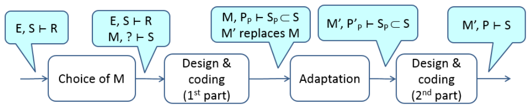
Figure 6 shows a process that takes into account the change of platform M occurring when the program has already been partly implemented, i.e., PP is available, such that together with M it implements a subset SP of specifications S. The adaptation activity (a sort of refactoring) converts PP into program P’P, which implements the same specifications SP as PP did, but running on M’. Finally, a second Design and coding stage enhances P’P to get a new program P that fully implements S running on M’.
By comparing Figure 4 with Figure 6, it is clear that if M changes, the overall development duration and effort increase by the amount required by the Adaptation activity. The number of platform changes that occur during the development is not known a priori, but it can be estimated, based on experience.
11. Software Properties and Measures
In this section, it is shown how to describe the properties of the software product in a way that is precise enough to support the definition of metrics. Robustness and usability are the two properties used as examples to illustrate the process.
11.1. Robustness
Robustness has been defined in several, more or less similar, ways:
The above definitions are somewhat ambiguous: what does it mean that the system has to behave “correctly” or “appropriately”? What are abnormal conditions, invalid inputs and stressful environmental conditions?
By making reference to formula E, S ⊢ R, it is possible to provide a precise definition of robustness.
In a normal development process, the environment is described by E, user requirements are described by R, and software development deals realizing P such that E, M, P ⊢ R holds. Actually, well written software development contracts explicitly report E and R, and usually mention M (e.g., to specify how/where the system has to be deployed). In particular, it is important that E is well specified, since many programs yield different results in different environments (i.e., operating conditions).
Robustness deals with the behavior of a program when used in conditions that do not comply with E. With the proposed notation, Robustness can be defined as
Definition (22) considers that the the hardware/software systems operates in conditions (described by Ex) that are broader than the originally envisioned conditions (described by E). Nonetheless, the outcomes (described by Rx), though possibly broader than the envisioned outcomes (described by R), are acceptable for the users.
Based on the notion of robustness defined by (22), it is possible to define measures that quantify how robust a system (M and P) is. Intuitively, a system is more robust if it behaves acceptably when the operating conditions are more distant form the originally envisioned ones. So,
In (23), the measure of robustness is defined as the maximum distance between the envisioned environment behavior E and the unexpected environment behaviour Ex for which the system still behaves acceptably. Assuming—as reasonable—that , (23) explicitly excludes the existence of environment behaviors that are at a greater distance from E and still let the system behave acceptably.
For instance, let us consider the following conditions:
- E specifies that no more than 10 users are ever simultaneously connected to the system;
- R prescribes that the response time of the system is not greater than 0.5 s.
- dist(Ex,E) indicates the number of connected users (in Ex) exceeding the maximum number stated in E (i.e., 10).
- Acceptable(Ex, E, Rx, R) indicates that when the number of users in Ex is greater than the maximum number of users in E, the maximum tolerable response time is 0.55.
Now, suppose that the following situation holds, e.g., because Rx indicates that the response time is 0.55 s, while Ry indicates that it is 0.6 s:
The measure of the robustness of the system indicates that two users more than the expected maximum number of users are tolerated by the system, while more than two cause the system’s performance to become unacceptable.
Similarly, one could specify via that the difference between the response time in Rx and R must not be greater than 0.04 times the difference between the users in Ex and E.
11.2. External Properties of Software: The Case of Usability
The external manifestations of software are described by S; accordingly, most properties of software are properties of S.
However, properties like usability involve also the behavior of users. Accordingly, usability is best assessed when considering the formula that highlights the behavior of users: EI, ED, S ⊢ R (2). So, usability can be evaluated via the analysis of ED in connection with S.
More precisely, we have
- Some operating conditions, as described in EI,
- People that operate as described in ED, to achieve one of the goals as described in R,
- People that operate as described in ED, interacting with the machine as described in S.
The interaction with the machine (in each operating condition and for each goal) can be observed, measured or assessed from the point of view of usability. A measure of usability can then be defined, based on the evaluations of each observed interaction. For instance, ED could need to generate a set of inputs and interpret a set of outputs, to achieve a specific goal in R: the number of inputs and outputs, and the time taken by ED to achieve the goal could contribute to a measure of the usability of the machine (P and M) with respect to the considered goal.
12. Conclusions
It is a general opinion that software engineering lacks a core theory. This paper has shown that entailment E, S ⊢ R, proposed by Jackson [3], can be used effectively to specify what software development is, and how it can be organized in terms of artifacts and activities.
In this paper, the considered formula was used to describe several life cycles. Different levels of descriptions were addressed: business needs, requirements, specifications and programs. Besides, it was shown that the formula can be used to explain various properties and relationships that link software artifacts.
Overall, it seems that formula E, S ⊢ R can be used to describe and explain many concepts and phenomena of software engineering in a quite straightforward way. It can also be considered a first step towards a unifying theory for software engineering, in that the same type of entailment can be used to describe relationships among different types of software artifacts in different life cycles.
So, the software engineering community should probably consider using this formula more extensively than has been done till now.
Funding
This research received no external funding.
Conflicts of Interest
The author declares no conflicts of interest.
Abbreviations
The following abbreviations are used in this manuscript:
| MDPI | Multidisciplinary Digital Publishing Institute |
| HW | Hardware |
| SW | Software |
| UAT | User Acceptance Test |
| TDD | Test Driven Development |
| YAGNI | “You Aren’t Gonna Need It ” |
| SEMAT | Software Engineering Methods and Theory |
| ISO | International Organization for Standardization |
| IEEE | Institute of Electrical and Electronics Engineers |
| LoC | Lines of Code |
| COCOMO | Constructive Cost Model |
References
- Royce, W.W. Managing the development of large software systems: concepts and techniques. In Proceedings of the Proceedings of the 9th international conference on Software Engineering, 1987; pp. 328–338. [Google Scholar]
- Sommerville, I. Software engineering – 10th Edition; Pearson, 2016. [Google Scholar]
- Jackson, M. The meaning of requirements. Ann. Softw. Eng. 1997, 3, 5–21. [Google Scholar] [CrossRef]
- ISO. Systems and Software Engineering, Software Life Cycle Processes ISO/IEC/IEEE 12207 First edition; International Organization for Standardization, 2017. [Google Scholar]
- McConnell, S. Rapid development: taming wild software schedules; Pearson Education, 1996. [Google Scholar]
- Washizaki, H. Guide to the Software Engineering Body of Knowledge v4.0a; IEEE Computer Society, 2025. [Google Scholar]
- Johnson, P.; Ekstedt, M.; Jacobson, I. Where’s the theory for software engineering? IEEE Softw. 2012, 29, 96–96. [Google Scholar] [CrossRef]
- Jacobson, I.; Ng, P.W.; McMahon, P.E.; Spence, I.; Lidman, S. The essence of software Engineering: applying the SEMAT kernel; Addison-Wesley, 2013. [Google Scholar]
- Hall, J.G.; Rapanotti, L. Beauty in software engineering. Computer 2013, 46, 85–87. [Google Scholar] [CrossRef]
- Jackson, M. Software Specifications and Requirements: a lexicon of practice, principles and prejudices; Addison-W esley: New York, 1995. [Google Scholar]
- Jackson, M. Problem Frames: Analyzing and structuring software development problems; Addison-Wesley Longman Publishing Co., Inc., 2000. [Google Scholar]
- Benington, H.D. Production of large computer programs. Ann. Hist. Comput. 2008, 5, 350–361. [Google Scholar]
- Theofanos, M.F.; Pfleeger, S.L. Wavefront: a goal-driven requirements process model. Inf. Softw. Technol. 1996, 38, 507–519. [Google Scholar] [CrossRef]
- Lavazza, L. Business goals, user needs, and requirements: A problem frame-based view. Expert Syst. 2013, 30, 215–232. [Google Scholar]
- Gunter, C.A.; Gunter, E.L.; Jackson, M.; Zave, P. A reference model for requirements and specifications. IEEE Softw. 2002, 17, 37–43. [Google Scholar]
- Fowler, M.; Highsmith, J.; et al. The agile manifesto. Softw. Dev. 2001, 9, 28–35. [Google Scholar]
- Project Management Institute (PMI). The Future of Project Work: Pulse of the Profession® 2024, 2024. [CrossRef]
- Takeuchi, H.; Nonaka, I.; et al. The new new product development game. Harv. Bus. Rev. 1986, 64, 137–146. [Google Scholar]
- Boehm, B.W. Verifying and validating software requirements and design specifications. IEEE Softw. 1984, 1, 75. [Google Scholar] [CrossRef]
- Knuth, D. Comment to Peter van Emde Boas. Available online: http://www-cs-faculty.stanford.edu/.
- Lions, J.L.; Luebeck, L.; Fauquembergue, J.L.; Kahn, G.; Kubbat, W.; Levedag, S.; Mazzini, L.; Merle, D.; O’Halloran, C. Ariane 5 flight 501 failure report by the inquiry board, 1996. Available online: https://www.csm.ornl.gov/.
- Pratt, V. Anatomy of the Pentium bug. In Proceedings of the Colloquium on Trees in Algebra and Programming, 1995; Springer; pp. 97–107. [Google Scholar]
- Boehm, B.W. Software engineering economics. IEEE transactions on Software Engineering, 1984; pp. 4–21. [Google Scholar]
- Albrecht, A. Function-Point Method (Measuring Applications Development Productivity). In Proceedings of the IBM Application Development Joint Share and Guide Symposium, Monterey, 1979. [Google Scholar]
- Boehm, B.W.; Abts, C.; Brown, A.W.; Chulani, S.; Clark, B.K.; Horowitz, E.; Madachy, R.; Reifer, D.; Steece, B. Software Cost Estimation With Cocomo II; Prentice Hall, 2000. [Google Scholar]
- IEEE. Std 610.12 - IEEE Standard Glossary of Software Engineering Terminology; 1990.
- ISO/IEC. ISO/IEC 14143-1:2007; Information technology – Software measurement – Functional size measurement – Part 1: Definition of concepts. 2007.
Figure 1.
The traditional representation of the waterfall life cycle.
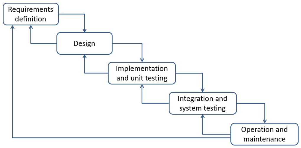
Figure 2.
The representation of the waterfall life cycle according to the proposed approach.
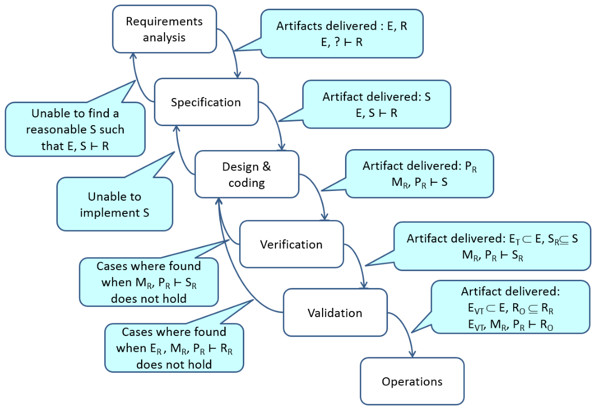
Figure 3.
The Design & coding activity.
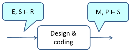
Figure 4.
A more detailed description of Design & coding activity.
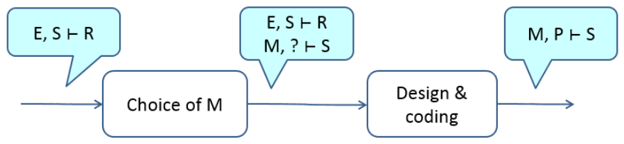
Figure 5.
Changing M affects the Design & coding activity.
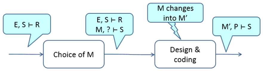
Figure 6.
Model including sub-activities required to account for M changing in the Design & coding activity.
Figure 6.
Model including sub-activities required to account for M changing in the Design & coding activity.
Disclaimer/Publisher’s Note: The statements, opinions and data contained in all publications are solely those of the individual author(s) and contributor(s) and not of MDPI and/or the editor(s). MDPI and/or the editor(s) disclaim responsibility for any injury to people or property resulting from any ideas, methods, instructions or products referred to in the content. |
© 2026 by the authors. Licensee MDPI, Basel, Switzerland. This article is an open access article distributed under the terms and conditions of the Creative Commons Attribution (CC BY) license (http://creativecommons.org/licenses/by/4.0/).
Copyright: This open access article is published under a Creative Commons CC BY 4.0 license, which permit the free download, distribution, and reuse, provided that the author and preprint are cited in any reuse.


