

Submitted:
10 July 2026
Posted:
13 July 2026
You are already at the latest version
Abstract
The inconsistency between the classical formula and the conventional relativistic formula for the Doppler effect in electromagnetic waves is revisited. The classical formula can be derived based on the hypothesis of phase invariance of a plane wave under the Galilean transformations, while the conventional relativistic formula can be derived based on the same hypothesis under the Lorentz transformations. In this paper, we propose to derive a Lorentz type relativistic formula for the Doppler effect by strictly solving the radiation fields of a moving Hertzian dipole with the Lorentz transformations and inverse Lorentz transformations. The resultant formula is exactly of the same form as the classical one instead of the conventional relativistic formula. Our analysis shows that the inconsistency is due to the fact that the angular frequencies defined in different frames have different bases because of time dilation. It may be more natural to evaluate the Doppler effect between the angular frequency of the source and that of the fields received by the observer in the same time base. Moreover, we have derived a general expression for the Doppler effect from the far field of a moving Hertzian dipole. The result clearly shows that the classical formula and the Lorentz type relativistic formula are approximate forms of the general formula by representing the far field with a plane wave.
Keywords:
Maxwell’s equations
; Doppler shift
; Hertzian dipole
; phase invariant
; Galilean transformations
; Lorentz transformations
1. Introduction
The Doppler effect describes the variation in the frequency of waves when the observer and the source of the wave have relative motions. Doppler effect may exist in all kinds of waves. This paper only concerns about the Doppler effect observed in the electromagnetic waves generated by the electromagnetic sources in free space.
There are mainly two types of formulae for the Doppler effect: the classical formula and the conventional relativistic formula [1,2,3,4,5]. In order to analyze the inconsistency existed between them, we are to re-derive them with transformations of the plane wave between inertial frames, as shown in Figure 1, where is the laboratory frame in which the observer is at rest, and is the rest inertial frame in which the source is at rest.
Assume that the electric field of the plane wave in the laboratory frame can be expressed by
where is the wave vector. Denote the phase of the plane wave as:
The classical formula for the Doppler effect can be derived using the Galilean transformations [1],
Making use of the hypothesis that the phase of the plane wave is invariant under the Galilean transformations, we can write that
Inserting (3) into (4) and equating the corresponding terms, we get and the classical formula for the Doppler effect,
where is the wavenumber, , and . Conventionally, the angular frequency at the rest reference frame is denoted as . In this case, . For the sake of comparison, we denote the angular frequency of the wave derived in this way as .
Einstein [4] derived the conventional relativity formula for the Doppler effect by making use of the Lorentz transformations (LTs),
where is the Lorentz factor. The subscript “⊥” and “||” represent the transversal and parallel component of the vector, respectively. Einstein has assumed that, in the laboratory frame , the electromagnetic waves at the observation point far away from the source can be represented to a sufficient degree of approximation by a plane wave. The phase of the plane wave is expressed by (2) and is invariant under the Lorentz transformations. By inserting (6) into (4), he obtained the relation between the wave vectors in the two frames,
and the relation between the angular frequencies in the two frames,
We have denoted in (8) to represent the angular frequency at the rest frame, and have denoted the angular frequency of the plane wave in the frame by to distinguish it from that in the classical formula (5). It is obvious that (8) differs from the classical formula (5) by a Lorentz factor . Einstein did not give explanations why the phase of plane wave should be invariant under the Lorentz transformations. Jackson [1] explained that the phase of a plane wave is an invariant quantity because the elapsed phase of a wave is proportional to the number of wave crests that have passed the observer. Since this is merely a counting operation without units, it must be independent of coordinate frame. However, this explanation also seems to lack solid theoretical foundation because it ignores the fact that the temporal period in the counting varies between inertial frames.
We should pay attention to two critical facts: one is that the above derivation is based on the hypothesis that the phase of a plane wave is invariant in all inertial frames; the other is that the Doppler effect is described by the relationship between the angular frequency of the fields in the frame and the angular frequency of the moving source in its rest frame . A very important fact has been ignored by researchers: is defined in with , while is defined in with , the time bases for their definition are not the same because of the time dilation effect. When we try to evaluate the Doppler effect in the waves far away from the source in the frame , it is more natural to compare the angular frequency of the moving source and the angular frequency of the fields in the same frame on the same time base. In other words, we should express in terms of the period instead of the proper period , namely,
where can be interpreted as the value of the angular frequency of the source when expressed in terms of the period in the frame . It is important to note that we have under the Galilean transformations, so we have in (5).
It may be more intuitive to discuss the issue using the frequency instead of the angular frequency . We can treat the frequency of the source as counting the number of the period per second. Because of the time dilation under the Lorentz transformations, . For the same source, when counted in , the number of period per second is ; when counted in , the number of period per second is . For example, we consider a harmonic source with period of . The frequency in is 10Hz, which means that we count 10 period () per second in . Assume that , then the proper period is . The frequency in is , which means that there are 20 proper period in one second when we count it in . The frequency of the source is 20Hz when it is measured in . However, its value is converted to 10Hz when it is evaluated in the frame . We should evaluate the Doppler effect by comparing the frequency of the fields we have measured in with 10Hz instead of 20Hz.
We may directly follow Einstein’s derivation and represent the fields far away from the source by a plane wave. However, instead of making use of the hypothesis of phase invariance, we derive the formula by rigorously applying the Lorentz transformations. Assume that the source is harmonically oscillating with and moves uniformly with velocity . The position of the source at time is . Its fields at the observation point can be approximately expressed with a plane wave with phase of . We are to find the relationship between and to reveal the Doppler effect. With Lorentz transformations, the position of the uniformly moving source is transformed to a fixed position in . The transformation of the time is , so the harmonically oscillating source becomes , where is a constant because is a fixed position vector. Therefore, the phase of the plane wave generated by the source in should be
from which we get . This verifies the correctness of (9).
In order to get the plane wave solution in the frame , we write the plane wave generated by the harmonic source in the frame as follows,
Note that in equation (11). We still use for the intrinsic impedance of the vacuum because the properties of the vacuum is not changed under Lorentz transformations.
Now we transform the plane wave from the frame to the frame with the inverse Lorentz transformations for the electromagnetic fields [9],
where is the inverse Lorentz transformations,
where is the identity operator. The space-time coordinates are transformed with (6). With the definitions of the vectors, we can verify that the electromagnetic field in the frame is still a plane wave. Its electric field can be expressed by , where the angular frequency is derived to be
To distinguish it from that in the conventional relativistic formula (8), we have denoted the angular frequency of the plane wave obtained with LTs by . Evidently, if derived with rigorous Lorentz transformations, the relativistic formula for Doppler effect is exactly of the same form with the classical formula (5) and not in consistent with the conventional relativistic formula (8). To distinguish them, the formula (14) is called Lorentz type relativistic formula for Doppler effect, which can be considered as the solution of moving point source obtained by solving the Maxwell’s equations with frame-hopping technique (FH) [9,11,12]. The inconsistency between the Lorentz type relativistic formula and the conventional relativistic formula for the Doppler effect is caused by the fact that the conventional relativistic formula is derived by directly applying the hypothesis of phase invariance of plane waves in all inertial frames instead of strictly applying the LTs and inverse LTs.
2. The General Formula for Doppler Effect Derived with Moving Hertzian Dipole
We have analyzed the electromagnetic radiation properties of a uniformly moving Hertzian dipole in the vacuum [6]. The dipole is modelled with two anti-phase harmonic charges with small spacing , where is the oscillating angular frequency of the charge. The electric dipole moment is expressed by . To satisfy the current continuity law, there should be a very short current filament with density of between the two charges. The polarization unit vector points from to . It is assumed that all the three sources move together with velocity in the direction perpendicular to , as shown in Figure 2.
The center of the Hertzian dipole is denoted by . The densities of the two moving charges can be expressed with the Dirac delta function as
Their motion induces two currents with densities of
The short current between the two charges also moves along the trajectory, and its current density becomes
When , the Liénard-Wiechert potentials [1,2,8] of the above moving sources have been solved in [6], from which the electromagnetic fields of the uniformly moving Hertzian dipole are derived to be
In the expressions, is the radius vector pointing from the source point to the observation point, , , and . In addition, and are respectively the permittivity and wavenumber in the vacuum. is a source-related constant. In the vacuum, the fields generated at propagates to the observer at with the light velocity . The governing equation for the wave propagation is,
from which we can solve based on the causality principle, and obtain that [6]:
where is the angle between the vector and .
At places far away from the source, we have . Based on (21) and making use of the causality principle, we can approximately express in terms of with [6]
The field of the moving Hertzian dipole at region far away from its birthplace can be written as
where
Equation (24) describes the relationship between the angular frequency of the far field and the angular frequency of the moving Hertzian dipole. It is extracted from the far fields that are obtained by solving the Maxwell’s equation in the laboratory frame without any frame transformations.
The fields of the uniformly moving Hertzian dipole have also been solved with the frame-hopping technique. At first, the space-time coordinates of the center of the Hertzian dipole are transformed into with LTs (6). The results are
Obviously, the center of the dipole is transformed to the origin of the frame . Since , we have . The moving velocity of the sources is transformed to . Consequently, the three source densities can be transformed into as follows,
Note that has no Lorentz contraction since . In particular, it is obvious that the angular frequency of the source is transformed from to , which once again justifies the relationship of (9).
The space-time coordinate of the observation position can be transformed into the space-time coordinate in the frame with LTs (6). The fields generated by the motionless Hertzian dipole in the frame are solved to be
In the expressions, , ,. The electromagnetic pulse generated at propagates to with velocity , hence, , from which we can obtain that
We can solve from (31) and check that
Substituting into (32), we can verify that the result is exactly the same as (21).
The fields and of the Hertzian dipole in the frame can be obtained with the inverse Lorentz transformations (12) for the electromagnetic fields. It has been proved that the fields obtained with Lorentz Transformations are exactly the same as those obtained with the Lienard-Wiechert potentials [8,10]. In addition, we have recently analyzed the scattered fields of uniformly moving PEC objects with the two methods. Our numerical results have demonstrated that the scattered fields obtained with the frame-hopping techniques and that with the Lienard-Wiechert potentials are in agreement with high accuracy even in situations when the PEC object moves as fast as [11,12]. These results suggest that the formula (24) derived from the far fields of the moving Hertzian dipole is a general relativistic formula for the Doppler effect. The classical formula and the Lorentz type relativistic formula are the approximate forms of (24) by letting , that is, representing the far field by a plane wave.
3. Discussions
The proposed Lorentz type relativistic formula for the Doppler effect is exactly of the same form as the classical formula, where the angular frequency of the fields and the angular frequency of the moving source are measured in the same frame . The formula is obtained by approximately representing the fields far away from the source with a plane wave, i.e., it is an approximate form of the formula (24) with .
As a matter of fact, some researchers have suggested that the conventional relativistic formula for the Doppler effect based on the phase invariance hypothesis might need to be rechecked [13,14]. However, their opinions have not attracted much attention because most of them failed to provide convincing theoretical solutions, and are simply criticized by being not in consistent with the Theory of Special Relativity (TSR). We would like to mention that those critics might have ignored the basic fact that the phase invariance of plane waves among inertial frames is not an axiom but a hypothesis that has not been proved with rigorous theory or verified with solid experimental results. We think that it is of significance to show that the it is possible to derive the relativistic formula for the Doppler effect with Lorentz transformations instead of making use of the hypothesis.
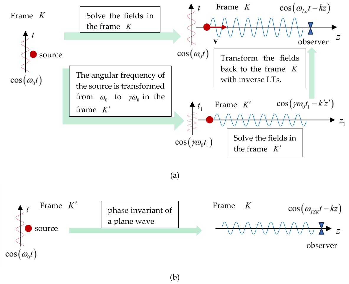
In order to give an intuitive illustration, we have schematically compared the relationships between the sources and waves in Figure 3. To Derive the Lorentz type formula, we have compared the angular frequency of the electromagnetic fields and that of electromagnetic source in the same frame, as shown in Figure 3(a). The electromagnetic fields are solved either through Lienard-Wiechert potentials, or with the frame-hopping methods. The two solutions are completely in agreement with each other. However, to derive the conventional relativistic formula, we have to compare the angular frequency of the electromagnetic fields in the laboratory frame and the angular frequency of the electromagnetic source in the frame based on hypothesis that the phase of a plane wave is invariant in all inertial frames.
When , there is no Doppler shift if we use the classical formula and the Lorentz type relativistic formula. However, if we use the conventional relativistic formula, there is a transversal Doppler shift due to the Lorentz factor . Denote and . When , we can derive from the conventional relativistic formula (8) that
The transversal Doppler occurs when , with a coefficient of 0.5 for the second order term of .
Historically, the transversal Doppler shift is regarded as a pure relativistic effect, and was expected to provide a critical experimental support for the TSR [15]. As a matter of fact, several experiments have been conducted to detect the relativistic Doppler effect [16,17,18,19,20]. As summarized in [20], there are mainly two types of experiments for measuring the relativistic Doppler shift. The first type is to take the arithmetic mean of the longitudinal Doppler shift at [18,19]. The experiments have reported a coefficient of [18] and [19]. The other type is to directly detect the relativistic Doppler shift at [20]. The experiment reported a coefficient of . These experiments seem to have confirmed the transversal Doppler shift predicted by TSR. However, we would like to mention that it is extremely difficult to align the observation angle accurately. Although the researchers had tried their best to improve the accuracy, the experimental results are still not accurately enough to reach a convincing verification. Including the relativistic correction in the GPS signals does not necessarily prove that the conventional relativistic formula is absolutely correct.
4. Conclusions
We have shown that the inconsistency between the Lorentz type relativistic formula and the conventional relativistic formula is caused by the fact that the reference angular frequency for the comparison is different. For the Lorentz type relativistic formula, the frequency of the electromagnetic fields observed in is compared with the frequency of the moving source in the same frame. On the contrary, the conventional relativistic formula is derived by comparing the frequency of the fields in the frame with the frequency of the moving source in the different frame . We have clearly demonstrated that the classical formula, which is exactly the same as the Lorentz type formula, is by no means the low-speed approximation of the conventional relativistic formula. In this paper, we just want to reveal the cause of the inconsistency between the Lorentz type relativistic formula and the conventional relativistic formula for the Doppler effect. We think that the inconsistency between the two kinds of formulas for the Doppler effect is one of the several inconsistencies between the Maxwell’s theory and TSR.
References
- Jackson, J.D. Classical Electrodynamics, 3rd ed; Wiley: New York, 1998. [Google Scholar]
- Chaichian, M.; Merches, I.; Radu, D.; Tureanu, A. Electrodynamics. An Intensive Course; Springer-Verlag: Berlin Heidelberg, 2016. [Google Scholar]
- Landau, L.D.; Lifshitz, E.M. The Classical Theory of Fields. In Elsevier Ltd, 4th ed.; Hamermesh, M., Translator; 1975; p. Chap.5. [Google Scholar]
- Einstein, A. On the electrodynamics of moving bodies, in The Principle of Relativity - A collection of original memoirs on the special and general theory of relativity; Dover Publications, Inc., 1923. [Google Scholar]
- Miller, A.I. Albert Einstein’s Special Theory of Relativity-Emergence (1905) and Early Interpretation (1905-1911); Springer: New York, 1997. [Google Scholar]
- Xiao, G.B. Re-interpreting the properties of the fields of a uniformly moving Hertzian dipole in the vacuum. Next Res. 2025, 2, 100856. [Google Scholar] [CrossRef]
- Field, J.H. Retarded electric and magnetic fields of a moving charge: Feynman's derivation of Lienard–Wiechert potentials revisited. Preprint 2015. [Google Scholar] [CrossRef]
- Xiao, G.B. Electromagnetic Sources and Electromagnetic Fields; Springer Nature: Singapore, 2024; Volume Chap. 3. [Google Scholar]
- Van Bladel, J. Relativity and engineering, 1st ed.; Springer: Berlin, Germany, 1984; pp. 70–72. [Google Scholar]
- Xiao, G.B. Solving the Fields of a Moving Hertzian Dipole with Frame-Hopping Method. IEEE Int. Conf. on Comput. Electromagnetics, Shanghai, China, Apr. 12, 2026. [Google Scholar]
- Liu, G.; Xiao, G.B.; Hu, M.; Zhu, J. Electromagnetic Scattering of Uniformly Moving PEC Objects-Part I: Integral Equation Formulations. IEEE Trans. Antennas Propag. 2026, 74, 5783–5792. [Google Scholar] [CrossRef]
- Liu, G.; Xiao, G.B.; Hu, M.; Zhu, J. Electromagnetic Scattering of Uniformly Moving PEC Objects-Part Ⅱ: Marching-on in Time Algorithm. IEEE Trans. Antennas Propag. 2026, 74, 5793–5805. [Google Scholar] [CrossRef]
- Renshaw, C. Explanation of the anomalous Doppler observations in Pioneer 10 and 11. IEEE Aerospace Conf. Proc. (Cat. No.99TH8403), Snowmass, CO, USA, 1999; vol.2, pp. 59–63. [Google Scholar]
- Thim, H.W. Absence of the Relativistic Transverse Doppler Shift at Microwave Frequencies. IEEE Trans. Instrument. Meas. 2003, 52, 1660–1664. [Google Scholar] [CrossRef]
- Zhang, Y.Z. Special relativity and its experimental foundation; World Scientific: Singapore, 1997. [Google Scholar]
- Ires, H.E.; Stilwell, G.R. An Experimental Study of the Rate of a Moving Atomic Clock. J. Opt. Soc. Am. 1938, 28, 215–226. [Google Scholar] [CrossRef]
- Ires, H.E.; Stilwell, G.R. An Experimental Study of the Rate of a Moving Atomic Clock. II. J. Opt. Soc. Am. 1941, 31, 369–374. [Google Scholar] [CrossRef]
- Mandelberg, H.I.; Witten, L. Experimental Verification of the Relativistic Doppler Effect. J. OPT. SOC. AM. 1954, 52, 529–536. [Google Scholar]
- Olin, A.; Alexander, T.K.; Hausser, O.; McDonald, A. B. Measurement of the Relativistic Doppler Effect Using 8.6-Mev Capture γ Rays. Phys. Rev. D. 1973, 8, 1633–1639. [Google Scholar] [CrossRef]
- Hasselkamp, D.; Mondry, E.; Scharmann, A. Direct observation of the transversal Doppler-shift. Z. Phys. A 1979, 289, 151–155. [Google Scholar] [CrossRef]
Figure 1.
Two reference frames. moves against with constant velocity .
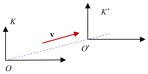
Figure 2.
Trajectory of a moving Hertzian dipole for .
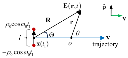
Figure 3.
Schematic illustration of Doppler effect. (a) Compare the angular frequency of the electromagnetic fields and electromagnetic source in the same frame. The electromagnetic fields are solved either through Lienard-Wiechert potentials, or with FH methods. (b) Compare the angular frequency of the electromagnetic fields in the laboratory frame and the angular frequency of the electromagnetic source in the frame based on hypothesis that the phase of a plane wave is invariant in all inertial frames.
Figure 3.
Schematic illustration of Doppler effect. (a) Compare the angular frequency of the electromagnetic fields and electromagnetic source in the same frame. The electromagnetic fields are solved either through Lienard-Wiechert potentials, or with FH methods. (b) Compare the angular frequency of the electromagnetic fields in the laboratory frame and the angular frequency of the electromagnetic source in the frame based on hypothesis that the phase of a plane wave is invariant in all inertial frames.
Disclaimer/Publisher’s Note: The statements, opinions and data contained in all publications are solely those of the individual author(s) and contributor(s) and not of MDPI and/or the editor(s). MDPI and/or the editor(s) disclaim responsibility for any injury to people or property resulting from any ideas, methods, instructions or products referred to in the content. |
© 2026 by the authors. Licensee MDPI, Basel, Switzerland. This article is an open access article distributed under the terms and conditions of the Creative Commons Attribution (CC BY) license (http://creativecommons.org/licenses/by/4.0/).
Copyright: This open access article is published under a Creative Commons CC BY 4.0 license, which permit the free download, distribution, and reuse, provided that the author and preprint are cited in any reuse.