
Submitted:
10 July 2026
Posted:
10 July 2026
You are already at the latest version
Abstract
Accurate ultra-short-term wind power forecasting at the turbine level is important for grid stability and dispatching. To address the time-varying spatial and temporal correlations among multiple turbines in a single wind farm, this paper builds dynamic spatio-temporal graphs to model dynamic spatial dependencies, proposes a causal dilated convolutional network to combine short-term and long-term dependencies, proposes a graph fusion layer to achieve weight fusion of different graph sources. Experiments show that GraphFusionGRU achieves the lowest error, outperforming compared baseline models. The results confirm the model’s improved robustness, and interpretability for complex wind farm environments.
Keywords:
wind power forecasting
; graph neural network
; dynamic multi-graph
; spatio-temporal modeling
; gated recurrent unit
1. Introduction
From the perspective of power system operation, the continuous growth of the installed capacity of wind power has improved its position in the power structure, but the large-scale integration of wind power has also brought new challenges to the safe and stable operation of the power grid. Wind power output is affected by wind speed, wind direction, air temperature, air pressure, unit operation status and other factors, with significant uncertainty, volatility and intermittency [1], which will affect the operation mode arrangement, frequency and peak shaving, reserve capacity configuration and power market output declaration. Therefore, how to accurately predict the change trend of wind power is an important issue to improve the capacity of new energy consumption and ensure the safe operation of power system.
According to the different prediction time scales, wind power prediction can generally be divided into ultra short-term prediction, short-term prediction and medium and long-term prediction. Among them, the ultra-short-term forecast is generally oriented to the next few minutes to several hours, mainly relying on the data of the supervisory control and data acquisition (SCADA) system of the wind farm to carry out modeling, which has direct guiding significance for real-time dispatching and station operation [2,3]. Compared with the day ahead prediction, the ultra-short-term prediction emphasizes the rapid response of local wind field changes, unit operation status and coupling relationship between wind turbines, so it puts forward higher requirements for the spatio-temporal feature extraction ability of the model.
WPF (Wind power forecasting) provides an important technical basis for the efficient accommodation of wind power and the secure operation of power grids. According to different modeling principles, existing forecasting methods can generally be divided into physics-based methods, statistical methods, data-driven methods, and physics-informed data-fusion methods. With the rapid accumulation of wind farm operational data, deep learning-based data-driven methods have become an important research direction in wind power forecasting.
In the last few years, deep learning methods are also being applied to wind power forecasting and include CNNs (Convolutional Neural Networks), RNNs (Recurrent Neural Network), and its variants. Since the CNNs can use local receptive fields well to capture temporal structure of wind power time series, whereas LSTMs (Long Short-Term Memory networks) have proven to be good at learning the long-term dependency of this kind of data [4,5]. To further boost forecasting results, some works integrate the CNN and LSTM together to build a hybrid model or an Encoder-Decoder architecture in order to extract both local feature and time-dependent information simultaneously [6,7].
In order to capture the long-term dependency, there are also plenty of multi-scale temporal modeling methods were proposed. Nguyen proposed a TCN (Temporal Convolutional Network) for multi-step wind power forecasting and enhanced the model’s stability by using residual connection [8]; Xu integrated bidirectional TCN with Transformer together in order to capture both forward and backward temporal feature [9]; Besides, self-attention has also shown its great performance on time series forecasting, due to the global modelling ability of Transformers are able to extract long range dependence from long sequence, which has shown great performance for multi-step forecasting task [10,11] .Some other recent time series forecasting model also improves the expression ability of complicated fluctuation by using multiscale feature fusion or multidimensional frequency domain information [12,13].
Except for deterministic forecasting. Due to the uncertainty of wind power generation, probability prediction methods are also increasingly receiving attention. Some researchers have conducted interval prediction and probability density WPF prediction of based on distribute modeling, kernel density estimation and quantile regression neural networks. These methods not only provide predicted values but also quantitatively describe prediction uncertainty, which is of great significance in power grid scheduling and risk analysis [14].
Although deep-learning-based methods have made substantial progress in WPF, most existing studies mainly model wind power as individual or independent time series and unable to completely capture the spatial correlations among the wind turbines. Therefore, introducing models capable of jointly characterizing temporal and spatial dependencies has become an important direction for further improving wind power forecasting performance.
Graph Neural Networks (GNN), which can encode entity and its interaction as graph, provides a powerful tool to capture complex spatial dependence among the wind turbines. In a wind farm, individual turbines could be treated as nodes, while inter-turbine interactions could be modeled as edges. Therefore, GNNs were increasingly adopted for wind power forecasting during past several years [15]. Spatio-temporal graph model was also widely employed for traffic flow forecasting, energy load forecasting [16], wind power forecasting [17]. For example, ASTGCN models intricate spatial– temporal relations through spatial attention, graph convolution, and temporal attention [18], while ST-Transformer also employs self-attention for capturing long-range spatial–temporal dependencies [19]. These works show that spatio-temporal graph learning is useful in modeling multi-step prediction problems; however, its performance often highly depends on the design of a good graph structure.
In early studies, graph structures were constructed only based on the geographical locations or Euclidean distances of wind turbines, where a fixed adjacency matrix was used to describe spatial relationships among turbines [20,21]. These methods are easy to implement and can introduce spatial information. However, because the graph structure is changing over time, such methods are unable to capture the dynamic coupling relationships among wind turbines.
To address this limitation on static graph, recently some researchers start to investigate dynamic graph construction approaches [22,23]. They build a dynamic graph structure with correlation coefficients or graph attention mechanism [24,25] and federated learning [26], and so on. These approaches are capable of describing the dynamic relationship between nodes by changing their interconnections when wind farm operation states change and it has been demonstrated that they could enhance the accuracy and robustness in the forecast.
However, a single type of graph is insufficient to characterize the complex interactions among wind turbines. For example, geographical distance graphs mainly describe spatial adjacency, windspeed correlation graphs reflect the correlation of wind speed variations, and power correlation graphs characterize the similarity of wind power fluctuation trends. Some studies combine multiple graph structures and use attention mechanisms or weighted fusion strategies to get multi-source spatial information [27,28]. Compared with single-graph modeling, multi-graph fusion methods can better describe the spatial heterogeneity of wind farms.
The recent works also improved the expressiveness for spatio-temporal modeling with more graph information coming from various sources [29]. Li et al. built multi-relation graphs, including the geographical distance map, the wind speed correlation map and the power correlation map, then they fused them adaptively via an attention mechanism [30]; Shang dynamically learn the cross-variable association by considering several variables as heterogeneous nodes [31]. The above works show that it is promising to model multi-sources graphs in order to improve the performance on wind power prediction.
On the other hand, there are some shortcomings in previous works about dynamic graph building and multi-graph fusing methods. Firstly, most of them adopt a relatively simple method to fuse one or more than one graph: which prevents full exploitation of the complementary information contained in multi-source spatial relations. Secondly, the adaptability of graph topologies are often limited especially on a node level resulting in insufficient adapting update capability under complicated operation scenarios for wind farms. Consequently, designing spatio-temporal forecasting models that are able to integrate heterogeneous graph structure and support nodewise adaptive modelling is still a crucial research topic in the field of wind power forecasting.
To sum up, the existing wind power prediction methods have made some progress in different scenarios, but there are still the following problems when facing the ultra-short-term prediction task of wind farm unit level.
First, some methods mainly focus on the changes of the time series, ignoring the spatial correlation between the wind turbines over time. In particular, a static graph model with fixed adjacency matrix is difficult to describe the dynamic correlation structure evolving with the change of wind speed, power fluctuation and operation state in the wind farm.
Second, a single graph structure is difficult to fully express the multi-source spatial relationship between wind turbines. The relationship between wind turbines is affected not only by geographical distance, but also by wind speed similarity, power coupling and local operating conditions. Using only one of the geographical map, wind speed map or power map, it is difficult to fully depict the complex spatial dependence inside the wind farm. Although the multi graph fusion method has been used in spatio-temporal prediction tasks, there is still room for further research on how to efficiently, stably and adaptively fuse multiple graph structures at the node level.
Third, although some dynamic graph methods introduce time-varying adjacency matrix, the construction basis and update mechanism of dynamic graph are still insufficient. For wind farm SCADA data, the relationship between wind turbines may be obviously nonlinear, and the statistical dependence may not be fully expressed only by using linear correlation or global learning adjacency matrix.
In view of the above problems, this paper takes the real wind farm SCADA data as the research object, and carries out research around dynamic spatial dependence construction, multi-source graph information fusion and unit level multi-step ultra short-term power prediction. The main contents of this paper are as follows.
(1) Aiming at the problem that the relationship between wind turbines varies with time and has nonlinear dependence, this paper proposes a dynamic adjacency matrix construction method based on normalized mutual information (NMI). The method calculates the nonlinear statistical dependence between wind speed series and power series in each fixed length historical time window, constructs the dynamic wind speed graph and dynamic power graph, and updates the graph structure with the sliding window to depict the time-varying spatial coupling relationship between wind turbines.
(2) Aiming at the problem that a single graph structure is difficult to fully describe the spatial relationship of multi-source wind farms, this paper constructs a multi graph spatio-temporal prediction framework integrating dynamic wind speed graph, dynamic power graph and static geographic distance graph. Among them, the dynamic wind speed graph is used to describe the similarity of meteorological variables, the dynamic power graph is used to describe the unit output coupling relationship, and the static geographic distance graph is used to provide a stable spatial proximity prior.
(3) Aiming at the problem that the existing multi graph fusion methods have insufficient node-adaptive capability, this paper designs a node level gated fusion mechanism. The multi-layer perceptron adaptively assigns the contribution weights of different graph structures according to the characteristics of nodes, so that the model can flexibly integrate multi-source spatial information for different wind turbine nodes and different operating states.
(4) In terms of the prediction model structure, this paper combines multi-scale time convolution, dynamic graph convolution and Gru decoder to build a joint spatio-temporal prediction model to achieve multi-step ultra short-term power prediction at the wind farm unit level. At the same time, this paper verifies the effectiveness, stability and rationality of the proposed method by comparing it with the traditional deep learning model, ASTGCN, St-transformer, DynamicGNN and other advanced spatio-temporal models, and combining ablation experiment, fusion strategy comparison, gat variant and directed graph variant experiments.
2. Materials and Methods
2.1. Graph Construction
The aim of this study is to predict wind turbine power output from 10 minutes to 4 hours.
Generally, wind power generation is affected by various factors. The basic physical relationship between wind speed and power generation follows:
In Eq. (1), the variables that determine the power generation are: air density , blade swept area , wind turbine operating efficiency and wind speed . In fact, the value of is also affected by .
Based on this relationship, we use wind speed , and power for each wind turbine arranged in chronological order:
Where and are the wind speed or power of turbine at time .
As Eq. (2) and according to the chosen time window length: H=144 (or 24 hours), the spatio-temporal correlation of features in each time window is calculated, the dynamic correlation matrix sequence of input features is formed.
2.1.1. Normalized Mutual Information
To model the complex spatio-temporal dependencies among the wind turbines, we use the NMI (Normalized Mutual Information) to construct time-varying graph structure. While many existing methods construct spatial graphs based on geographic distance, fixed neighborhood, or linear similarity metrics such as cosine similarity or Pearson correlation, such graphs are often static and unable to model dynamic and nonlinear interactions of wind turbines.
We use NMI to construct dynamic graphs, which enables more adaptive and expressive modeling of complex spatio-temporal dependencies between wind turbines.
As Figure 1 shows, and respectively represent the sequence within the time window of turbine and , then the marginal entropy and joint entropy of the variables are defined as:
The mutual information is defined as:
To eliminate the difference in entropy scale between different nodes, this paper adopts a normalized form:
In practical calculations, continuous wind speed and power sequences are discretized into several equally wide bins, and then the edge and joint probability distributions are estimated. Finally, a dynamic adjacency matrix can be constructed:
denotes the correlation of turbine and at time .
The resulting adjacency value in Eq. (6) quantifies the correlation strength between turbines and in this window. During the processing of one window, this adjacency matrix remains fixed; therefore, it can be regarded as a static graph for the current sample.
The dynamic NMI adjacency matrices are updated on a per-sample-window basis. With the given data resolution of 10 min, the historical input window length H = 144, corresponding to 24 h.
The dynamic graphs are updated once for each sliding input window. When the sliding stride is one time step, the update frequency is 10 min. During both training and inference, only historical observations within the current input window are used to construct the dynamic graphs, and no future information from the prediction horizon is involved. During one multi-step forecasting process, the adjacency matrices remain unchanged; they are recalculated only when a new observation window becomes available.
2.1.2. Euclidean Distance
To incorporate the spatial proximity between turbines, we also construct a static geographical graph based on Euclidean distance. Assuming that the wind farm with wind turbines, its coordinate matrix is:
In Eq. (7), represents the plane coordinates of the wind turbine .
The spatial distance matrix between wind turbines is defined by Euclidean distance in Eq. (8):
Set , in order to convert distance information into similarity strength, this paper uses a Gaussian kernel to map distance to dimensionless spatial weights:
Notably, the coordinate information is not directly used as an input feature; instead, it is only used for building the static spatial graph , is the median distance between all turbines. This method is relatively robust and is not easily affected by extremely large distance or abnormal coordinates.
2.2. Temporal Feature Extraction
Along the temporal dimension, a dilated TCN is used to extract multi-scale features from the time series of each node. TCN expands the receptive field while maintaining temporal order through dilated convolution.
Figure 2.
Dilated Convolution.
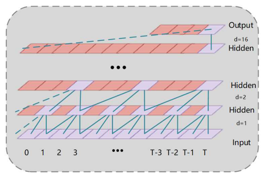
Figure 3.
Framework of TCN.
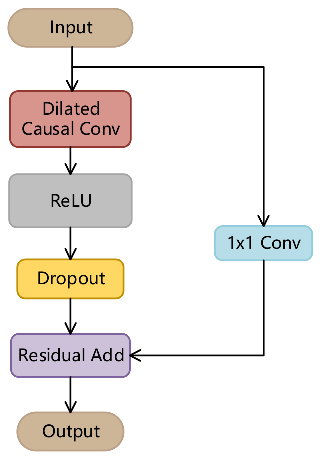
Let the input wind turbine node sequence be , where is the batch size, is the time length, is the number of nodes, and is the input feature dimension.
For node , its time series after multiple layers of dilated convolution:
2.3. Graph Fusion
Given that different spatial graphs may exhibit varying importance across turbines and time periods, a simple global fusion strategy is insufficient to capture spatial heterogeneity in large wind farms.
While wake propagation between wind turbines is a physically directed process, we construct graphs that represent only effective statistical dependencies and not an actual wake-causality path; specifically, the dynamic wind-speed and power plots use normalized mutual information that quantifies the mutual dependence strength of two turbine time series in a historical window. As mutual information is defined to be symmetric, the resulting adjacency matrices are naturally undirected pairwise association descriptions. Similarly, the geographical graph is derived from the Euclidean distances and describes a symmetric spatial proximity.
To further examine the graph aggregation mechanism, a GAT-based variant was added by replacing the GCN module with a GAT module while keeping the temporal encoder, dynamic graph construction, multi-graph fusion mechanism, and GRU decoder unchanged.
2.3.1. Graph Convolution on Multiple Graphs
To capture the spatial dependency relationships between wind turbine nodes, we design a spatial modeling module based on GCN, which integrates multiple graph structures. To capture spatial dependencies from multiple sources, we employ three types of graph structures:
(1) A dynamic wind-speed graph series,
(2) A dynamic power-correlation graph series ,
(3) A static geographic-distance graph.
At time step , the node features are , and the corresponding weighted adjacency matrix is . The standard graph convolution operation is defined as:
In Eq. (12), is the adjacency matrix with self-loops and normalization, is the learnable weight matrix, is the nonlinear activation
In Eq. (13) is the degree matrix.
Graph convolution is performed on the three types of graphs in Eq. (14):
2.3.2. Node-Level Gating Fusion Mechanism
After obtaining spatial features from multiple graphs, we design a node-level gating fusion module to adaptively combine them. This module integrates the output of static geographic convolution and the output of two dynamic convolutions and .
In Figure 4, for the time series of a certain node, we construct a fusion gating vector:
In order to improve computational efficiency and avoid high dimensionality, the feature concatenation at the beginning and end of the time window is selected as input, and three weight distribution are generated through MLP:
The final fused spatial features are:
In Eq. (17), represents the element-wise multiplication weighted by nodes.
This node-level fusion allows each turbine to assign different weights for the three graphs, enabling spatial heterogeneity modeling and improving the robustness of long-sequence training.
2.4. Gated Recurrent Unit
GRU, the Gated Recurrent Unit, is also one of the variants of the traditional RNN model.
As shown in Figure 5: it is mainly consists of two gates:
The reset Gate :
Used to control the proportion of information from the past and new input in the current hidden layer.
The update Gate :
Controls whether information about previously hidden layers is ignored.
The hidden layers are computed as:
Which denotes the bias and is the calculated weight.
3. Proposed Method
For the typical WPF task, the goal of this study is to jointly integrate the spatial correlation, time dependence, and geographic information among wind turbines within the wind farm into a unified model to improve the accuracy and stability.
As Figure 6 shows, the proposed method combines TCN, multi-graph gate fusion GCN, and GRU. For data preprocessing, we performed outlier detection and correction to improve the quality of input data. The input consists of 144 steps of historical wind speed and power to create the time window, structured as 4D tensors. Based on this, NMI dynamic graphs can be constructed. The node features are then passed to three parallel GCNs:
(1) Dynamic wind-based adjacency, (2) Dynamic power-based adjacency, (3) Static geographical distance.
Given the input size 144, to capture temporal patterns, we apply dilated TCN with kernel size [3,9,27,81], enabling multi-scale receptive fields. The dilation factor increases by a factor of 3 at each layer.
These heterogeneous spatial features are combined using a node-level gated fusion mechanism, where a two-layer MLP with Softmax activation outputs adaptive weights to merge the three graph outputs per node and time step.
The fused spatio-temporal features are unfolded and send into a sequence and then fed into a GRU-based decoder, which performs multi-step forecasting of future turbine power outputs over the next 24 steps.
Table 1 provides key implementation details, including dimensions and training hyperparameters.
4. Discussion
The experimental evaluation is designed to answer the following questions: (1) whether the proposed method outperforms existing baselines; (2) how the model behaves under long-horizon forecasting; (3) the necessity of each architectural component; and (4) the interpretability of the graph fusion mechanism.
Extensive experiments were conducted on a real wind farm dataset. The dataset was obtained from the Spatial Dynamic Wind Power Forecasting Competition at Baidu KDD Cup 2022. The dataset covers 134 wind turbines in Longyuan Wind Farm, with a total of 245 days of operating data on wind speed, direction, power, temperature. The data resolution is 10 minutes. This work only uses wind speed and power data for input.
As shown in Figure 7, compared with wind speed and historical power, the direction-related variables show much weaker direct linear correlation with power output. In particular, the Pearson correlation coefficient between the wind-direction cosine component and power is approximately 0.11. This does not imply that wind direction or wake propagation is physically unimportant. Rather, it suggests that the available wind-direction signal does not provide stable and strong additional predictive information under the current data quality and forecasting setting.
4.1. Spatio-Temporal Correlation Dynamic Graph
To make the dynamic graph convolutional network more robust, firstly, we obtain the spatio-temporal correlation between wind turbines based on massive training samples and then during the learning process, the model uses such a previously calculated dynamic mutual information matrix as the instance-level adjacency matrix to conduct graph convolution operation. Note that since no abrupt change occurs in WFP, the spatial correlation among them is still a smoothly varying function.
As shown in Table 2 and Figure 8, from the perspective of structural correlation, the average structural correlation of the dynamic graphs of Wind and Power is consistent (ρ=0.9632), but the results show the difference between the two under dynamic trends compared to the average results (ρ=0.8449 ± 0.0757), indicating that NMI’s correlation calculation captures different data trends. In addition, the Power graph exhibits greater changes in the time dimension, reflecting stronger dynamic response capabilities.
Compared to static geographic graphs, both dynamic graphs have lower correlation (ρ≈ 0.3), indicating that they provide temporal structural information beyond spatial adjacency. This not only reduces the impact of redundant noise, but also provides more comprehensive information for the prediction model.
4.2. Experimental Setup
Data preprocessing was completed and outlier identification and processing have been carried out as described earlier. The input time window length is set to 144 steps (24 hours), the predicted output length is set to 24 steps (4 hours), and the model is set to predict power values for the next 24 steps using historical input data.
All models are implemented using the PyTorch 2.5.1+cu124 framework, and training and inference are performed on servers equipped with NVIDIA RTX 4090 (24GB) and 16 vCPU Intel(R) Xeon(R) Gold 6430. The data is divided into training set, validation set, and test set in chronological order, with proportions of 70%, 15%, and 15% respectively.
4.3. Evaluation Metrics
To avoid order effects during training, the loading order of the training set is shuffled. The evaluation metrics are listed below:
NMAE (Normalized Mean Absolute Error), is defined as follows: the average of the absolute value of the difference between the predicted value and the actual value.
NRMSE (Normalized Root Mean Square Error), is the square root of the average of the squares of the difference between the predicted value and the actual value.
In Eq. (22) and Eq. (23), is the actual value and is the predicted value.
Cohen’s dz is an effect size for paired repeated measurement data. It measures the standardized improvement of the proposed method over the baseline. of proposed method compared with baseline method after standardization.
In Eq. (24), if >0, the baseline error is larger than the proposed-method error, generally speaking, when this value is greater than 0.2, it indicates that there is a small effect, greater than 0.5 is a medium effect, and greater than 0.8 is a large effect.
4.4. Simulation Results and Discussion
4.4.1. Basic Analysis
To fairly compare and analyze the performance among various time series prediction models for ultra short-term WPF, we compare proposed method with following baselines, GRU, LSTM, Transformer, TimeMixer, TimeNet, XGBoost, ASTCGN, ST-Transformer, DynaimcGCN, with our proposed method GraphFusionGRU. The power prediction curve is shown as follows:
Figure 9.
Power Forecasting Curves for All Methods.
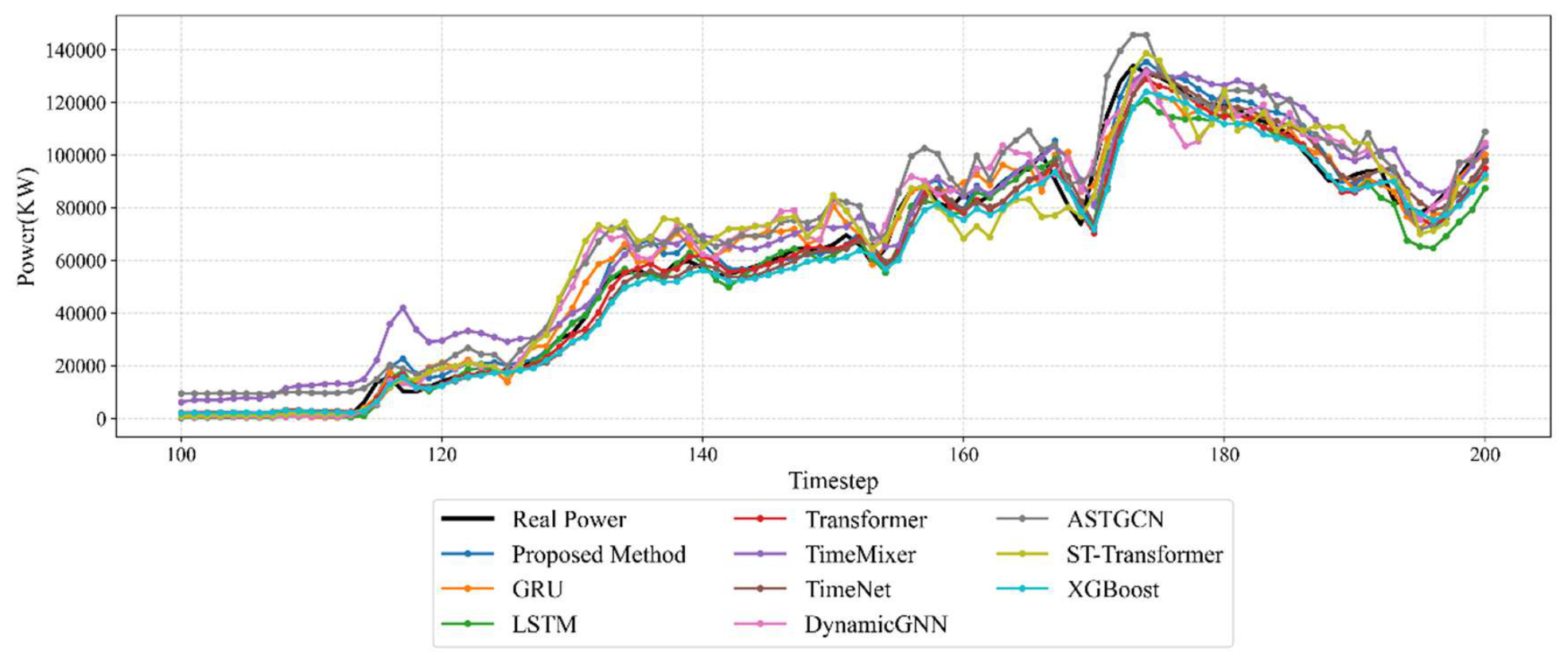
To validate the statistical reliability of the experiment, we run all methods five times using different random seeds. As Table 3 shows, the proposed method achieves 6.85%±0.11% NMAE, 9.68%±0.08% NRMSE, indicating that the proposed method is superior to various comparative models in terms of overall prediction accuracy.
Compared with the traditional time series model, proposed method shows clear advantages. For example, compared with GRU, LSTM, Transformer, TimeMixer and TimeNet, proposed method has achieved 6.39%, 8.33%, 7.33%, 8.79% and 7.49% improvements in NMAE, respectively.
Especially, DynamicGNN is the closest method to the proposed method among all baseline models. The result shows that dynamic graph modeling plays an important role. However, it remains difficult to fully describe the multi-source spatial relationship between wind turbines by relying only on a single dynamic graph structure.

Table 4.
Comparison of metric results of different models (NRMSE).
| Metric | Mean | Std. | Improvement (%) | Cohen dz | P value t-test | Significant at 0.05 |
| Proposed | 9.68 | 0.08 | ||||
| ASTGCN | 10.73 | 0.23 | 9.77 | 2.58 | 4.47E-3 | TRUE |
| DynamicGNN | 9.98 | 0.06 | 3.05 | 1.69 | 1.93E-2 | TRUE |
| GRU | 10.34 | 0.09 | 6.35 | 3.39 | 1.63E-3 | TRUE |
| LSTM | 10.32 | 0.72 | 6.24 | 0.86 | 1.30E-1 | FALSE |
| ST-Transformer | 10.74 | 0.13 | 9.89 | 2.99 | 2.59E-3 | TRUE |
| TimeMixer | 10.45 | 0.18 | 7.36 | 3.77 | 1.09E-3 | TRUE |
| TimeNet | 10.14 | 0.36 | 4.54 | 3.81 | 1.04E-3 | TRUE |
| Transformer | 10.09 | 0.31 | 4.08 | 3.18 | 2.07E-3 | TRUE |
In addition, the results of the significance test indicate that the proposed method demonstrates strong advantage on both metrics. For NMAE, the improvement of proposed method over all other models except DynamicGNN, reached a significant level (p < 0.05). For NRMSE, statistical significance was also observed in the comparisons of all other models except LSTM. At the same time,the results of Cohen’s dz further show that the improvement of the proposed method has more obvious effect than that of most baseline models.
4.4.2. Time Horizon Analysis
Figure 10 and Table 5 and Table 6 further show the error curve of the model within the prediction time step range of 10 minutes to 4 hours. From the overall trend, the prediction error of each model increased gradually with the increase of the forecasting horizons from 10 min to 4 h. This is because the longer the forecasting horizon, the stronger the uncertainty caused by future wind speed changes, unit operation state fluctuations and error accumulation, and the more difficult accurate forecasting becomes.
In the case of short forecasting horizons, such as 10 min and 30 min, some time series models achieve low error. For example, the NMAE and NRMSE of TimeNet and Transformer under 10 min prediction are lower than the model in this paper. This shows that in the very short-term prediction scenario, the short-term autocorrelation of the power series is strong, and satisfactory forecasting performance can be achieved only by relying on the recent time trend.
However, as the forecasting horizon increases, the advantage of the proposed model becomes more evident. Under the 2 h, 3 h and 4 h forecasting horizon size, the model in this paper achieved the optimal results in NMAE and NRMSE. For example, under the 4-hour prediction, the NMAE of this model is 9.74%, which is lower than that of GRU, LSTM, Transformer, DynamicGNN, ASTGCN and ST-Transformer; The NRMSE was 12.52%, which also achieved the lowest error. This shows that when the prediction task is extended from a very short time to a longer horizon, it is difficult to maintain a stable prediction by relying only on the time trend of an individual turbine, while the dynamic spatial dependence and multi-source graph information between wind turbines become more important to improve the prediction stability.
Therefore, the results of Table 5 and Table 6 show that the main advantage of this model is not the absolute optimization of all short forecasting horizons, but the improvement of overall multi-step prediction performance and stability under the long prediction horizon. This result is also consistent with the original intention of the model design in this paper, that is, the dynamic NMI graph and multi graph fusion mechanism are used to enhance the representational capability of the model for the time-varying spatial coupling relationship of wind farms.
4.5. Ablation Study
To assess the contributions of model components, we designed an ablation study. Table 7 lists the configurations of ablation methods derived from the proposed method.
These variants are grouped along two dimensions:
(1) Effect of Spatio-temporal Components
Ablation-Temporal removes spatial modeling by replacing GCN with TCN only, effectively degrading the model to a pure temporal structure.
Ablation-Graph disables the TCN module, using GRU directly on graph-enhanced features.
As shown in Table 8 and Figure 11, these ablation methods perform worse than the proposed method. Ablation studies further demonstrate the effect of components of the proposed method. As the NMAE results show, proposed method is 6.85%, lower than other ablation baselines. Ablation-Temporal removes GCN, its NMAE is 7.09%, This indicates that multi-scale time convolution can effectively extract local and multi-scale temporal features from wind speed and power sequences. Ablation-Graph removes TCN, its NMAE is 7.14%, also higher than that of the proposed method. This indicates that relying solely on temporal feature extraction cannot sufficiently describe the spatial correlation among wind turbines.
(2) Effect of Graph Construction
Static-Graph replaces dynamic graphs with static ones, removing temporal adaptivity. Wind-only, Power-only and Geo-only explore the use of single-source graphs (wind, power, or distance) to evaluate the value of heterogeneous graphs.
The result of single-source graph models demonstrate that Wind-only, Power-only, Geo-only methods have larger prediction errors than proposed method, indicating that a single graph structure cannot fully characterize the complex internal spatial correlations in the wind farm.
Note that the Wind-only and Geo-only have higher error than proposed method, which means wind-speed and geographical relation plays an important role on prediction. In contrast, the Power-only method has a relatively high error.
In addition, the GAT method has 7.22% NMAE and 9.87% NRMSE, both are higher than those of the proposed method. This indicates that directly replacing GCN with a graph attention mechanism does not lead to stable improvements. A possible reason is that proposed method has already explicitly characterized the statistical correlations between wind turbines by dynamic NMI adjacency matrices. Introducing attention aggregation would lead to increased model complexity and introduce more uncertainty.
(3) Fusion Mechanism Comparisons
To explore alternatives to the MLP-based gating mechanism, we designed the alternative studies. Table 9 lists the configurations of alternative models derived from the proposed method:
Table 9 and Figure 12 indicate that MLP based gating performs the best, while the highest error for the Residual approach shows that simply adding features like a residual style cannot help to differentiate which structure contributes more. Which may lead to mutual interference of spatial information from different sources. The Attention fusion method can learn the weight between graphs to a certain extent, which leads to a better performance compared with Residual fusion. Nevertheless, it is still inferior to our proposed method. The possible reason lies in that traditional attention fusion focuses more on the whole weight learning which can not sufficiently learn the different demands of various wind turbine nodes towards specific graph structure.
Based on the results, we observe that the performance gain of proposed method does not come from one specific component. Preliminary results show that overall average metrics of proposed method are better than traditional time-series-based model as well as majority of state-of-the-art spatio-temporal graph models. The result for different prediction horizon also shows that the proposed method is more robust when predicting long horizons. Ablation study proves the importance of GCN, dynamic graph modelling, multi-graph structure and MLP gated fusion. Comparison of different fusion strategies shows that the node-level adaptive fusion is superior to the residual, fusion methods based on attention and fixed weight-based.
It should be noted that, the proposed model is not always superior to all baselines on very small horizons, suggesting that temporal autocorrelation still has a strong influence on short term prediction tasks. Thus, the benefit of the proposed model should be interpreted as improvement in general average performance and multistep prediction robustness, instead of global optimality over the entire horizon.
4.6. Interpretability Analysis
As shown in Figure 13, at different time steps, as the real power (or wind speed) increases, the weight of the geographical graph increases synchronously, while the weight of the wind speed and power graphs decreases. This confirms that the MLP fusion mechanism has the ability to dynamically allocate weights to different graphs based on different conditions.
Figure 14 shows the spatial heterogeneity of the wind farm: overall, geographic location relationships or wind turbine arrangement order dominate the weight allocation of most turbines for the three graphs, demonstrating that node-level gating captures the true spatial dependency patterns.
5. Conclusions
To address ultra-short-term WPF, this paper proposes a dynamic multi-graph fusion method based on NMI, dynamic graph construction, multi-scale time convolution and node-level gating fusion. The proposed model achieves better overall average performance across most forecasting horizons while some of the baselines are still competitive for very short horizons.
We plan to investigate clustering methods to lower the computational burden for large scale applications in future work.
Author Contributions
Conceptualization, M.C. and P.J.; methodology, P.J.; software, P.J.; validation, P.J.; formal analysis, P.J.; investigation, P.J.; resources, M.C.; data curation, P.J.; writing—original draft preparation, P.J.; writing—review and editing, M.C. and P.J.; visualization, P.J.; supervision, M.C.; project administration, P.J.; funding acquisition, M.C. All authors have read and agreed to the published version of the manuscript.
Funding
This research received no external funding.
Institutional Review Board Statement
Not Applicable.
Data Availability Statement
The data presented in this study are available on request from the corresponding author. The original contributions presented in the study are included in the article. Further inquiries can be directed to the corresponding author(s).
Conflicts of Interest
The authors declare no conflicts of interest.
Appendix A. Hyperparameter Sensitivity Analysis
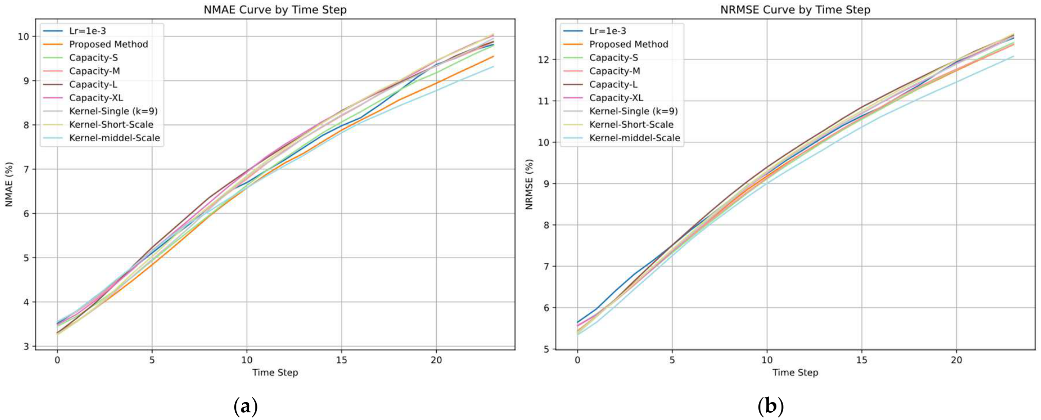
To demonstrate the robustness of the proposed method to hyperparameters, we conduct a sensitivity analysis by varying key hyperparameters. The hyperparameters used as follow:
Table A1.
Evaluation indicators Curve for Sensitivity Analysis.
| Category | Setting | NMAE (%) | NRMSE (%) |
| Baseline | Proposed (Default) | 6.85±0.15 | 9.57±0.07 |
| Learning rate | LR=1e−3 | 6.94 | 9.77 |
| Capacity | Capacity-S (TCN Hidden=16 GCN Hidden=32 RNN=64) | 6.87 | 9.62 |
| Capacity-M (TCN Hidden =24 GCN Hidden =48 RNN=96) | 7.02 | 9.64 | |
| Capacity-L (TCN Hidden =32 GCN Hidden =64 RNN=128) | 7.07 | 9.83 | |
| Capacity-XL (TCN Hidden =48 GCN Hidden =96 RNN=192) | 7.09 | 9.73 | |
| Kernel | TCN Kernel = [9] | 6.96 | 9.74 |
| TCN Kernel = [3,5,7] | 7.03 | 9.78 | |
| TCN Kernel = [9,27,81] | 6.76 | 9.43 |
As shown in Table A1 and Figure. A1, the performance remains within a narrow range across different configurations, which indicates that the proposed method does not rely on finely tuned hyperparameters.
Figure A1.
Evaluation indicators Curve for Sensitivity Analysis by 1–16 steps in advance (a)NMAE, (b)NRMSE.
Figure A1.
Evaluation indicators Curve for Sensitivity Analysis by 1–16 steps in advance (a)NMAE, (b)NRMSE.
Appendix B. Cross-Validation Results
In order to further test the time robustness of the proposed model, we conducted a cross-validation experiment. Fold0 corresponds to the default dataset partition used in this paper. For fold1-3, the test set remains unchanged, while the original training set (70%) is further divided into different training-validation partitions along the time axis, and all folds use the same test set.
Table A2.
Evaluation indicators Curve for Cross-Validation Results.
| Fold | 1 | 2 | 3 | 0 | ||||
| Model | NMAE | NRMSE | NMAE | NRMSE | NMAE | NRMSE | NMAE | NRMSE |
| Proposed Method | 9.81% | 13.21% | 9.60% | 12.98% | 9.09% | 12.55% | 6.85% | 9.57% |
| GRU | 10.08% | 13.96% | 9.51% | 13.48% | 9.85% | 13.69% | 7.45% | 10.34% |
| LSTM | 10.03% | 13.48% | 10.16% | 13.84% | 10.16% | 13.68% | 8.00% | 11.61% |
| TimeMixer | 9.95% | 13.76% | 10.11% | 13.78% | 10.23% | 14.06% | 7.46% | 10.48% |
| TimeNet | 9.81% | 13.10% | 9.61% | 13.21% | 9.71% | 13.32% | 7.28% | 10.00% |
| XGBoost | 9.99% | 14.29% | 9.82% | 14.00% | 10.05% | 14.55% | 7.55% | 10.80% |
| Transformer | 10.34% | 13.51% | 9.91% | 13.28% | 9.32% | 14.55% | 7.53% | 10.16% |
As shown in the table, the performance of the proposed model in different folds generally maintains the advantages over other methods, which indicates that the proposed method is insensitive to the specific training verification segmentation in the training data compared with other models.
Appendix C. Transfer Generalization
To evaluate the generalization ability of the proposed method for different wind farms, we conducted an experiment on the public wind power dataset consisting of 200 turbines located in the mainland United States.
As shown in Table A3, the proposed method consistently achieves lower NRMSE and NMAE compared with baseline methods.
Table A3.
Evaluation indicators of Transfer Generalization (1h ahead).
| Methods | NRMSE | NMAE |
| GRU | 18.07% | 10.64% |
| LSTM | 18.83% | 12.32% |
| TimeMixer | 20.31% | 13.76% |
| TimeNet | 19.46% | 12.40% |
| Transformer | 18.28% | 10.81% |
| XGBoost | 18.83% | 12.25% |
| Wind-only | 18.12% | 10.34% |
| Power-only | 18.14% | 10.29% |
| Geo-only | 18.14% | 10.30% |
| Proposed Method | 17.87% | 10.21% |
References
- Vanderwende, B.J.; Lundquist, J.K. The modification of wind turbine performance by statistically distinct atmospheric regimes. Environ. Res. Lett. 2012, 7(3), 034035. [Google Scholar] [CrossRef]
- Yang, M.; Huang, Y.; Guo, Y.; et al. Ultra-short-term wind farm cluster power prediction based on FC-GCN and trend-aware switching mechanism. Energy 2024, 290, 130238. [Google Scholar] [CrossRef]
- Huo, J.; Xu, J.; Chang, C.; et al. Ultra-short-term wind power prediction model based on fixed scale dual mode decomposition and deep learning networks. Eng. Appl. Artif. Intell. 2024, 133, 108501. [Google Scholar] [CrossRef]
- Yuan, X.; Chen, C.; Jiang, M.; et al. Prediction interval of wind power using parameter optimized beta distribution based LSTM model. Appl. Soft Comput. 2019, 82, 105550. [Google Scholar] [CrossRef]
- Gu, B.; Zhang, T.; Meng, H.; et al. Short-term forecasting and uncertainty analysis of wind power based on long short-term memory, cloud model and non-parametric kernel density estimation. Renew. Energy 2021, 163, 687–708. [Google Scholar] [CrossRef]
- Chen, Y.; Wang, Y.; Dong, Z.; et al. 2-D regional short-term wind speed forecast based on CNN-LSTM deep learning model. Energy Convers. Manag. 2021, 244, 114451. [Google Scholar] [CrossRef]
- Wang, Y.; Wei, S.; Yang, W.; et al. Construction of offline predictive controller for wind farm based on CNN-GRNN. Control Eng. Pract. 2022, 114, 105290. [Google Scholar] [CrossRef]
- Nguyen, H.K.M.; Phan, Q.-D.; Wu, Y.-K.; Phan, Q.-T. Multi-step wind power forecasting with stacked temporal convolutional network (S-TCN). Energies 2023, 16, 3792. [Google Scholar] [CrossRef]
- Xu, W.; Dai, W.; Li, D.; Wu, Q. Short-term wind power prediction based on a variational mode decomposition–BiTCN–Psformer hybrid model. Energies 2024, 17, 4089. [Google Scholar] [CrossRef]
- Xiao, H.; He, X.; Li, C. Multi-step prediction of offshore wind power based on Transformer network and Huber loss. Int. J. Electr. Power Energy Syst. 2024, 162, 110229. [Google Scholar] [CrossRef]
- Pan, X.; Wang, L.; Wang, Z.; et al. Short-term wind speed forecasting based on spatial-temporal graph Transformer networks. Energy 2022, 253, 124095. [Google Scholar] [CrossRef]
- Wang, S.; Wu, H.; Shi, X.; et al. TimeMixer: Decomposable multiscale mixing for time series forecasting. arXiv 2024, arXiv:2405.14616. [Google Scholar]
- Nie, Y.; Nguyen, N.H.; Sinthong, P.; et al. A time series is worth 64 words: Long-term forecasting with transformers. arXiv 2022, arXiv:2211.14730. [Google Scholar]
- Jian, Y.; Shuai, Y.; Xuejun, C.; et al. Short-term wind power forecasting and uncertainty analysis based on hybrid temporal convolutional network. J. Eng. Sci. Technol. Rev. 2023, 16(2), 10. [Google Scholar] [CrossRef]
- Veličković, P.; Cucurull, G.; Casanova, A.; et al. Graph attention networks. arXiv arXiv:1710.10903.
- Bruninx, K.; Delarue, E. A statistical description of the error on wind power forecasts for probabilistic reserve sizing. IEEE Trans. Sustain. Energy 2014, 5(3), 995–1002. [Google Scholar] [CrossRef]
- Wu, D.; Gao, C. Short-term wind power generation forecasting based on the SVM-GM approach. Electr. Power Compon. Syst. 2019, 46(11–12), 1250–1264. [Google Scholar] [CrossRef]
- Wang, L.; Gao, J.; Li, Y.; Wang, D. A method for ultra-short-term wind power forecasting of large-scale wind farms based on adaptive spatiotemporal graph convolution. Renew. Energy 2025, 249, 123321. [Google Scholar] [CrossRef]
- Sun, S.; Liu, Y.; Li, Q.; Wang, T.; Chu, F. Short-term multi-step wind power forecasting based on spatio-temporal correlations and transformer neural networks. Energy Convers. Manag. 2023, 283, 116916. [Google Scholar] [CrossRef]
- Zhao, Y.; Pan, S.; Zhao, Y.; et al. Ultra-short-term wind power forecasting based on personalized robust federated learning with spatial collaboration. Energy 2024, 288, 129847. [Google Scholar] [CrossRef]
- Lin, S.; Wang, S.; Xu, X.; et al. GAOformer: An adaptive spatiotemporal feature fusion Transformer utilizing GAT and optimizable graph matrixes for offshore wind speed prediction. Energy 2024, 292, 130404. [Google Scholar] [CrossRef]
- Peng, X.; Li, Y.; Tsung, F. A graph attention network with spatio-temporal wind propagation graph for wind power ramp events prediction. Renew. Energy 2024, 121280. [Google Scholar] [CrossRef]
- Wang, Z.; et al. Short-term wind speed forecast based on dynamic spatio-temporal directed graph attention network. Appl. Energy 2024, 361, 122071. [Google Scholar] [CrossRef]
- Duntoye, O.E.; Alowonou, K.C.; Kwon, D.-H. Wind power forecast using multilevel adaptive graph convolution neural network. Energies 2026, 19, 186. [Google Scholar]
- Wang, B.; Wang, Z.; Cao, X.; et al. Short-term wind power prediction with improved spatio-temporal modeling accuracy: A dynamic graph convolutional network based on spatio-temporal information and KAN enhancement. Electronics 2026, 487. [Google Scholar] [CrossRef]
- Hou, G.; Li, Q.; Huang, C. Spatiotemporal forecasting using multi-graph neural network assisted dual domain transformer for wind power. Energy Convers. Manag. 2025, 325, 119393. [Google Scholar] [CrossRef]
- Wang, F.; Chen, P.; Zhen, Z.; et al. Dynamic spatio-temporal correlation and hierarchical directed graph structure based ultra-short-term wind farm cluster power forecasting method. Appl. Energy 2022, 327, 119579. [Google Scholar] [CrossRef]
- Xu, M.; Zhu, R.; Yu, C.; Mi, X. DHGAR: Multi-variable-driven wind power prediction model based on dynamic heterogeneous graph attention recurrent network. Appl. Sci. 2025, 1862. [Google Scholar] [CrossRef]
- Peng, S.; Guo, L.; Huang, H.; et al. ForecastNet wind power prediction based on spatio-temporal distribution. Appl. Sci. 2024, 14(2), 937. [Google Scholar] [CrossRef]
- Li, T.; Liu, X.; Lin, Z.; et al. Ensemble offshore wind turbine power curve modelling: An integration of isolation forest, fast radial basis function neural network, and metaheuristic algorithm. Energy 2022, 239. [Google Scholar] [CrossRef]
- Shang, X.; Wei, Y.; Wan, D.; et al. A comprehensive cleaning method for outliers in wind turbine power curves based on the quartile method and segmented regression detection method. Energies 2026, 19, 1161. [Google Scholar] [CrossRef]
Figure 1.
Dynamic Spatio-temporal Correlation Calculation.
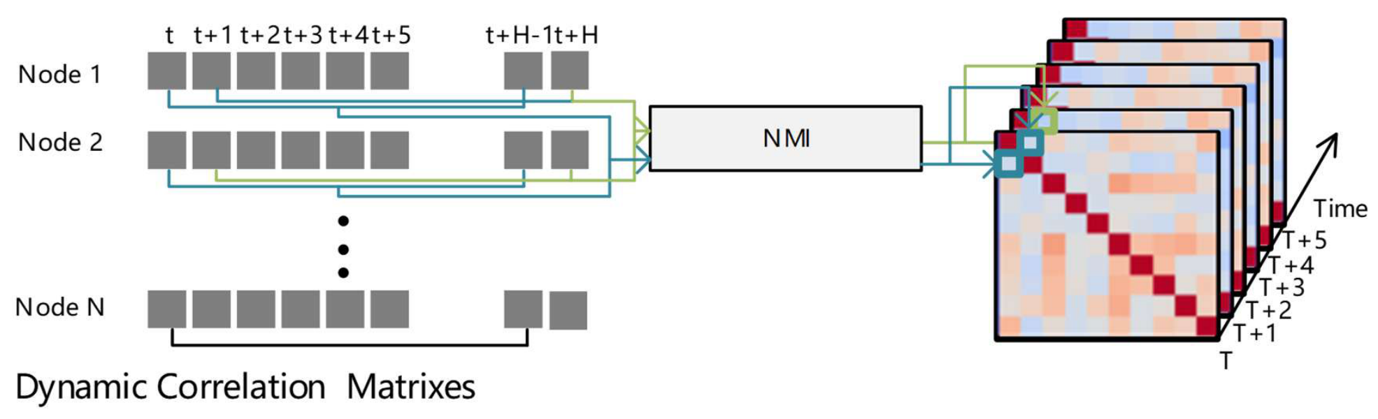
Figure 4.
Framework of Graph Fusion.
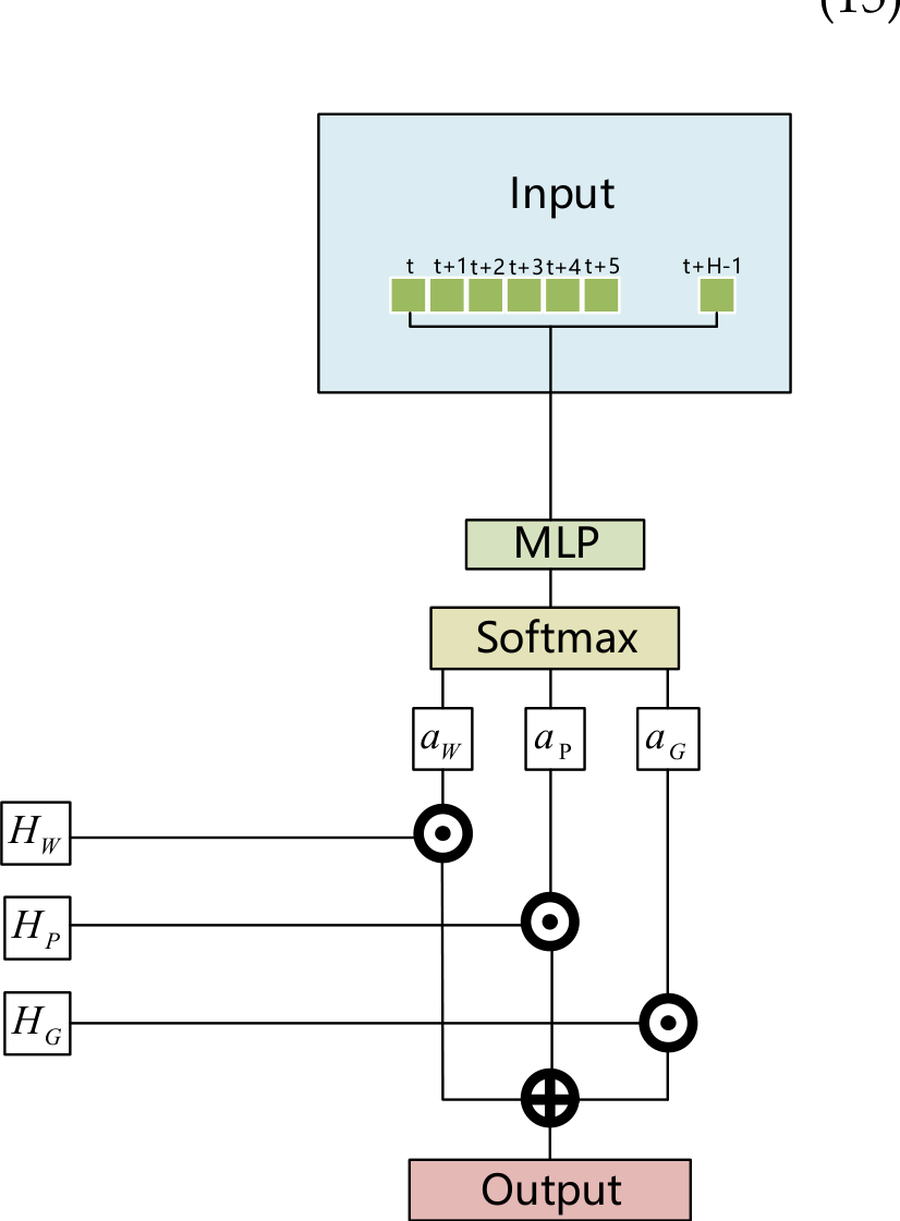
Figure 5.
Schematic Diagram of GRU.
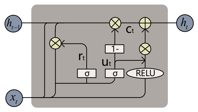
Figure 6.
Framework of Proposed Method.
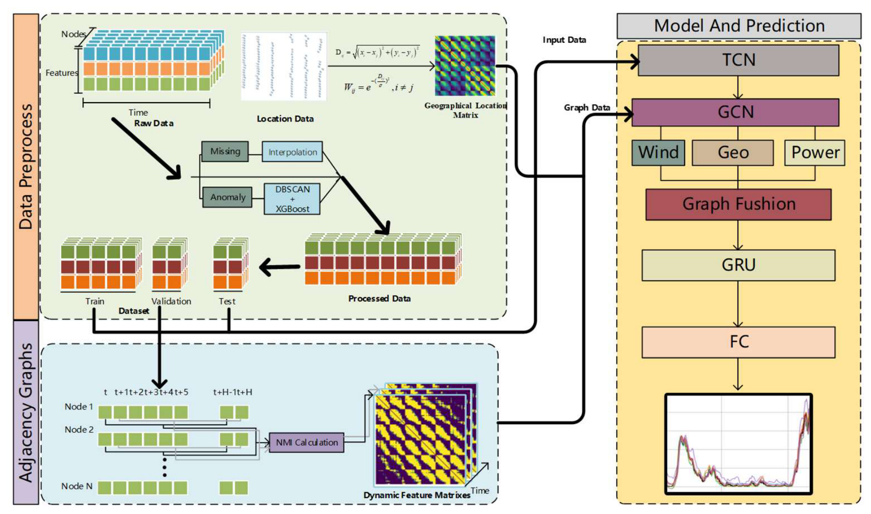
Figure 7.
Pearson Correlation of Features.
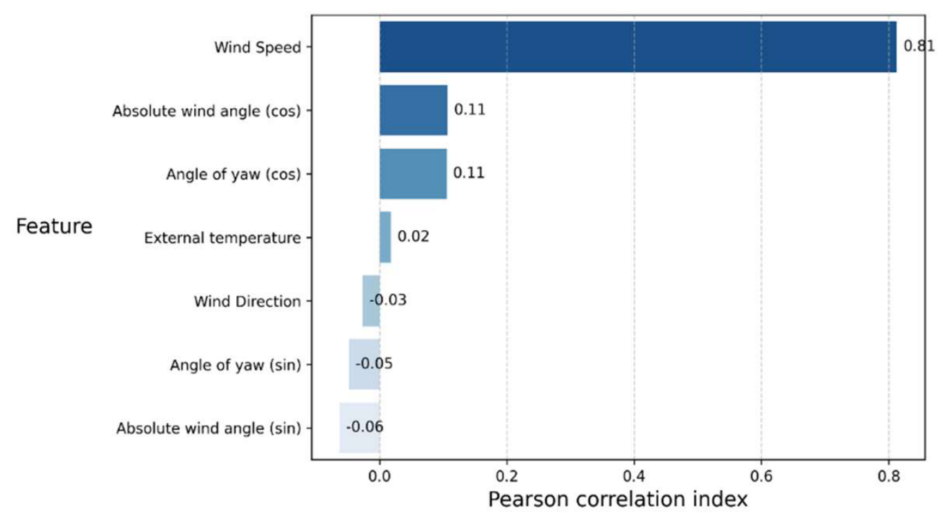
Figure 8.
Average correlation Graph of (a)Wind speed, (b)Power, (c)Location.
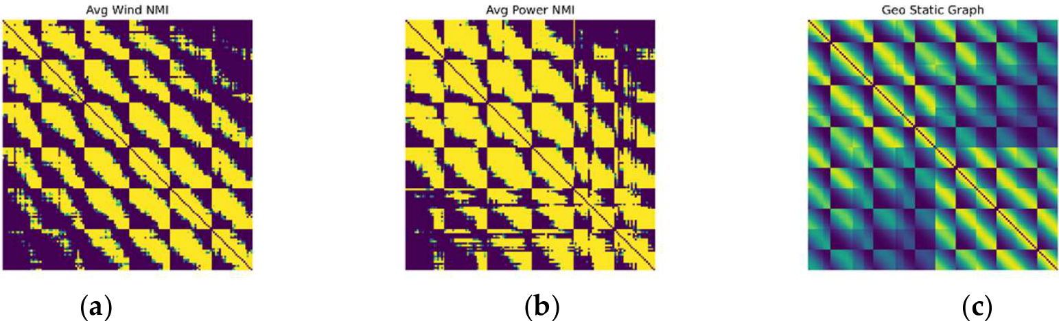
Figure 10.
Evaluation Metric Curves for ultra-short-term power prediction of the wind farm by 1–16 steps in advance (A)NMAE, (B)NRMSE.
Figure 10.
Evaluation Metric Curves for ultra-short-term power prediction of the wind farm by 1–16 steps in advance (A)NMAE, (B)NRMSE.
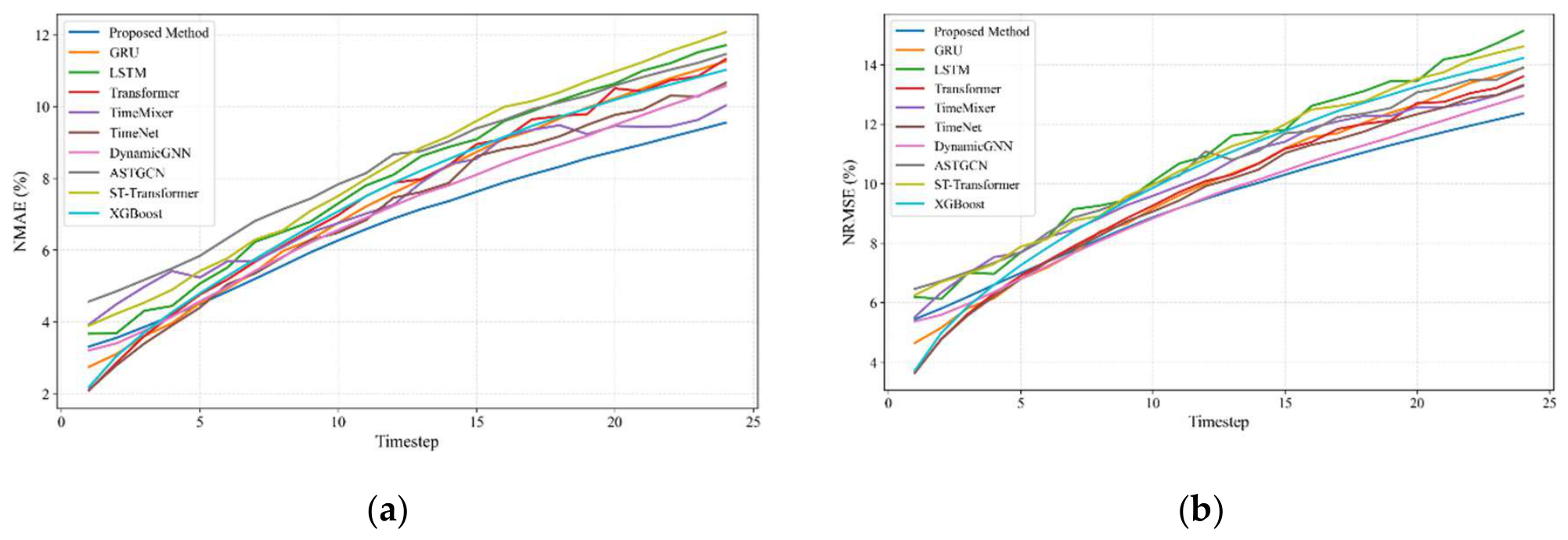
Figure 11.
Evaluation indicators Curve for Ablation study by 1–16 steps in advance(A)NMAE, (B)NRMSE.
Figure 11.
Evaluation indicators Curve for Ablation study by 1–16 steps in advance(A)NMAE, (B)NRMSE.
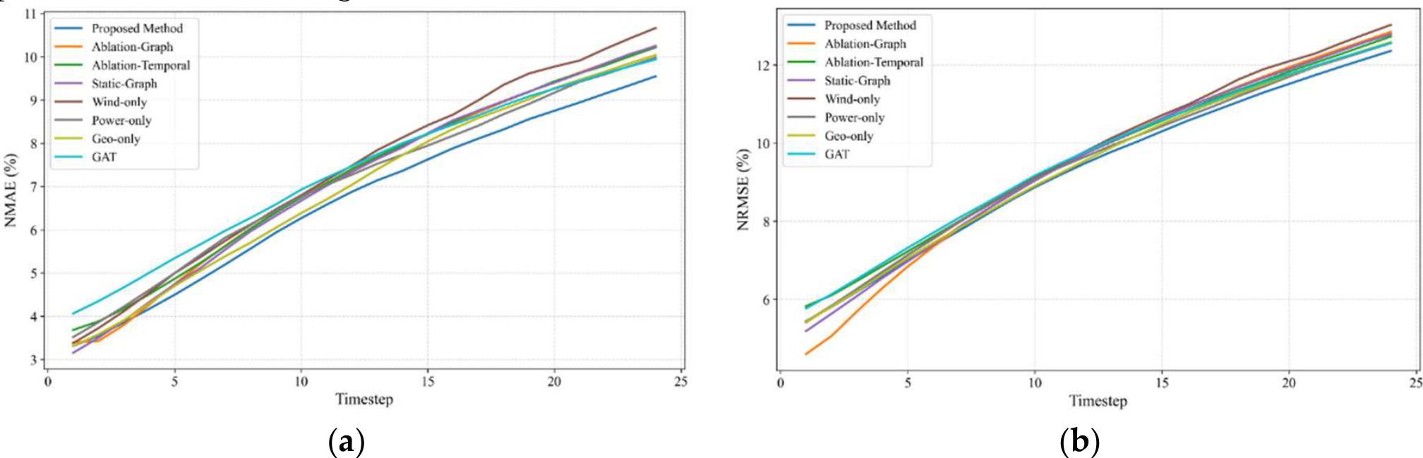
Figure 12.
Evaluation indicators Curve for Fusion Mechanism Comparisons by 1–16 steps in advance (a)NMAE, (b)NRMSE.
Figure 12.
Evaluation indicators Curve for Fusion Mechanism Comparisons by 1–16 steps in advance (a)NMAE, (b)NRMSE.
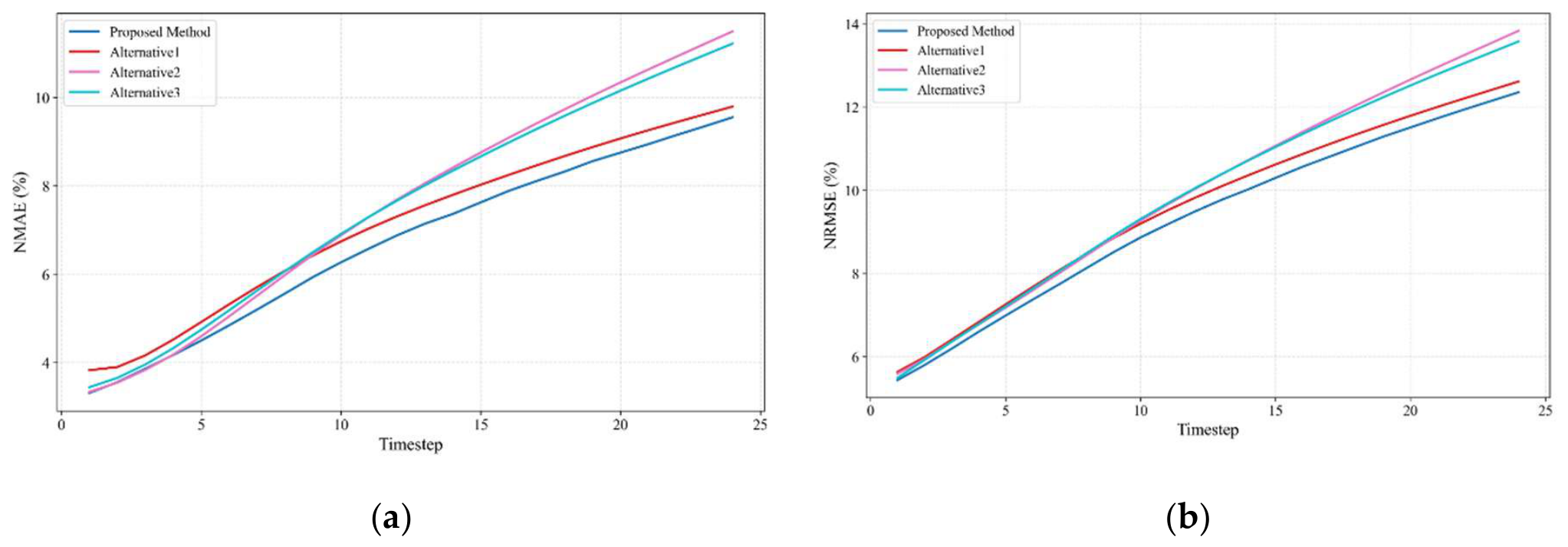
Figure 13.
Gate Weight of different time steps.
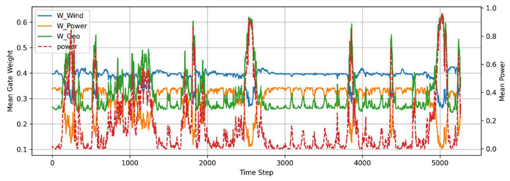
Figure 14.
Average Gate Weight of different wind turbines.
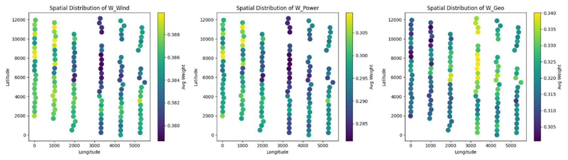
Table 1.
Implementation Details.
| Component | Parameter | Value | Description |
| Input | Window / Horizon | 144 / 24 (steps) | 24h history → 4h ahead prediction |
| Feature Dimension | 2 | Wind speed + Power | |
| Multi-Scale TCN | Kernel Sizes / Dilation | [3,9,27,81] / 1 | Multi-scale causal convolution |
| Output Dim | 64 | Fused via 1×1 conv | |
| Graph Fusion | Graphs | Wind, Power, Geo | Three dynamic/static graphs |
| Fusion Method | Learnable gated weights | Node-wise fusion via softmax gate | |
| Gate MLP Hidden | [128,64] | Two-layer gating network | |
| GRU Decoder | Input / Hidden Dim | N × 64 / 64 | RNN over temporal-graph fused features |
| Output Projection | Linear (hidden, 24×N) | Predict all 24 future steps | |
| Residual Mode | Baseline | Last / Mean of last 3 steps | Optional; for short-term residual correction |
| Data | Shape | [B, 144, N, 2] → [B, 24, N, 1] | Batch × Time × Nodes × Feature / Output |
| Training | Optimizer / LR | Adam / 1e-4 | Weight decay 2e-4, Reduce LR On Plateau scheduler |
| Loss Function | MSELoss | Early stopping (patience=10) | |
| Batch Size | 64 | For training, validation, test sets |
Table 2.
Metrics of Dynamic Matrices.
| Metrics | Wind-Power corr | Wind Avg Var | Power Avg Var | Dynamic Avg corr | Wind-Geo corr | Power-Geo corr |
| statistic | 0.9632 | 0.063952 | 0.092219 | 0.8449 ± 0.0757 | 0.2849 | 0.3157 |
Table 3.
Comparison of metric results of different models (NMAE).
| Metric | Mean | Std. | Improvement (%) | Cohen dz | P value t-test | Significant at 0.05 |
| Proposed | 6.85 | 0.11 | ||||
| ASTGCN | 7.84 | 0.21 | 12.67 | 1.42 | 3.03E-2 | TRUE |
| DynamicGNN | 7.05 | 0.12 | 2.77 | 0.88 | 1.20E-1 | FALSE |
| GRU | 7.32 | 0.2 | 6.39 | 1.87 | 1.38E-2 | TRUE |
| LSTM | 7.47 | 0.31 | 8.33 | 1.54 | 2.62E-2 | TRUE |
| ST-Transformer | 7.64 | 0.18 | 10.32 | 1.74 | 1.78E-2 | TRUE |
| TimeMixer | 7.51 | 0.25 | 8.79 | 3.24 | 1.92E-3 | TRUE |
| TimeNet | 7.41 | 0.7 | 7.49 | 4.06 | 8.17E-4 | TRUE |
| Transformer | 7.39 | 0.39 | 7.33 | 2.96 | 2.71E-3 | TRUE |
Table 5.
Comparison of NMAE results of different models and different time horizons (%).
| Horizon | 10min | 30min | 1h | 2h | 3h | 4h |
| Proposed | 3.41 | 3.93 | 4.94 | 6.96 | 8.5 | 9.74 |
| GRU | 2.74 | 3.51 | 4.84 | 7.47 | 9.48 | 11.07 |
| LSTM | 3.06 | 3.65 | 4.97 | 7.59 | 9.65 | 11.23 |
| TimeNet | 2.23 | 3.64 | 5.21 | 7.75 | 9.5 | 10.83 |
| TimeMixer | 3.64 | 4.52 | 5.52 | 7.69 | 9.33 | 10.43 |
| Transformer | 2.16 | 3.52 | 5.19 | 7.71 | 9.53 | 11.08 |
| Dynamic GNN | 3.66 | 3.93 | 4.78 | 7.04 | 8.9 | 10.38 |
| ASTGCN | 4.4 | 4.84 | 5.86 | 7.99 | 9.5 | 10.78 |
| ST-Transformer | 3.92 | 4.31 | 5.3 | 7.65 | 9.57 | 11.07 |
Table 6.
Comparison of NRMSE results of different models and different time horizons (%).
| Horizon | 10min | 30min | 1h | 2h | 3h | 4h |
| Proposed | 5.61 | 6.29 | 7.45 | 9.58 | 11.2 | 12.52 |
| GRU | 5.06 | 6.24 | 7.44 | 10.13 | 12.16 | 13.96 |
| LSTM | 5.35 | 6.1 | 7.42 | 10.07 | 12.17 | 13.97 |
| TimeNet | 3.76 | 5.69 | 7.49 | 10.13 | 11.99 | 13.45 |
| TimeMixer | 5.24 | 6.65 | 8.08 | 10.44 | 12.16 | 13.46 |
| Transformer | 3.68 | 5.64 | 7.47 | 10.06 | 11.94 | 13.52 |
| Dynamic GNN | 6.03 | 6.46 | 7.55 | 9.76 | 11.58 | 13.14 |
| ASTGCN | 7.06 | 7.34 | 8.49 | 10.75 | 12.11 | 13.55 |
| ST-Transformer | 6.55 | 7.17 | 8.22 | 10.41 | 12.28 | 14.00 |
Table 7.
Basic configuration of methods used in Ablation study .
| Methods | Category | Graph | Fusion | Graph | Ablation |
| Proposed Method | STGCN+GRU | Dynamic | MLP | Multigraph | Proposed |
| Ablation-Graph | GCN+GRU | Dynamic | MLP | Multigraph | w/o TCN |
| Ablation-Temporal | TCN+GRU | No | No | Multigraph | w/o GCN |
| Static-Graph | STGCN+GRU | Static | MLP | Multigraph | w/o Dynamic |
| Wind-only | STGCN+GRU | Dynamic | No | Wind | w/o Power & Geo |
| Power-only | STGCN+GRU | Dynamic | No | Power | w/o Wind & Geo |
| Geo-only | STGCN+GRU | Static | No | Geo | w/o Wind & Power |
| GAT | STGAT+GRU | Dynamic | MLP | Multigraph | GAT |
Table 8.
Basic Comparison of metric results of methods used in Ablation study.
| Baseline | Metric | Baseline mean | Improvement % | Cohen dz |
| Proposed | NMAE | 6.85 | ||
| Ablation-Graph | 7.14 | 3.99 | 0.84 | |
| Static-Graph | 7.16 | 4.32 | 1.02 | |
| Ablation-Temporal | 7.09 | 3.42 | 0.56 | |
| Geo-only | 6.98 | 1.78 | 0.41 | |
| Power-only | 7.19 | 4.71 | 1.19 | |
| Wind-only | 6.94 | 1.35 | 0.31 | |
| GAT | 7.22 | 5.15 | 1.84 | |
| Proposed | NRMSE | 9.68 | ||
| Ablation-Graph | 9.75 | 0.75 | 0.36 | |
| Static-Graph | 9.84 | 1.67 | 0.79 | |
| Ablation-Temporal | 9.92 | 2.45 | 0.96 | |
| Geo-only | 9.79 | 1.13 | 0.65 | |
| Power-only | 9.89 | 2.11 | 1.28 | |
| Wind-only | 9.77 | 0.90 | 1.01 | |
| GAT | 9.87 | 1.96 | 1.54 |
Table 9.
Comparison of metric results of different models for fusion methods.
| Baseline | Metric | Mean | Improvement (%) | Cohen dz |
| Proposed | NMAE | 6.85 | ||
| Residual | 7.3 | 6.22 | 1.42 | |
| Attention | 7.11 | 3.71 | 0.56 | |
| Fixed Weight | 6.98 | 1.9 | 0.53 | |
| Proposed | NRMSE | 9.68 | ||
| Residual | 10.03 | 3.47 | 1.36 | |
| Attention | 9.91 | 2.32 | 0.81 | |
| Fixed Weight | 9.82 | 1.41 | 1.32 |
Disclaimer/Publisher’s Note: The statements, opinions and data contained in all publications are solely those of the individual author(s) and contributor(s) and not of MDPI and/or the editor(s). MDPI and/or the editor(s) disclaim responsibility for any injury to people or property resulting from any ideas, methods, instructions or products referred to in the content. |
© 2026 by the authors. Licensee MDPI, Basel, Switzerland. This article is an open access article distributed under the terms and conditions of the Creative Commons Attribution (CC BY) license.
Copyright: This open access article is published under a Creative Commons CC BY 4.0 license, which permit the free download, distribution, and reuse, provided that the author and preprint are cited in any reuse.


