
Submitted:
09 July 2026
Posted:
10 July 2026
You are already at the latest version
Abstract
Using the properties of GL(2,R) matrices and the Chebyshev polynomials, we study the properties of several random fields of mutually dependent random variables (“spins”), indexed by finite onedimensional lattices forming closed chains. In any of these cases, we suppose the existence of a group of random variables, i.e., a “unit cell” of p ∈ N random variables with characteristics, which repeat itself along the chain. If p = 1 this leads to the model, called in physical sciences the one-dimensional Ising model. If p = 2 one has the so-called alternating Ising model. In any of these models the random variables can take only ±1 values (see the text for a precise definition). The couplings, that describe the mutual influence of two adjacent random variables can be both positive, enhancing the probability two adjacent variables to be of the same sign, or negative, when the opposite is true. Utilising the recurrence relations of Chebyshev polynomials and the bijective map between the number of spins and the polynomial index, we derive the free energy and specific heat in any of the models, discussing, for p ̸= 1, the specific heat double-Schottky anomaly.
Keywords:
dependent random variables
; mutual probability distributions
; probability theory
; statistical mechanics
; Ising model
; average values
; correlation functions
; Chebyshev polynomials
; Schottky anomaly
MSC: 82B20; 82M12
1. Introduction
In the current article we demonstrate how some properties of the matrices, together with those of the Chebyshev polynomials, can be used to study several Ising-type models with non-uniform couplings.
Variants of the one-dimensional Ising model with non-uniform couplings have been investigated extensively, both because of their physical relevance (see, e.g. [1] and refs. therein), and because of their rich mathematical structure ( see, e.g. [2], and refs. therein). The main difficulty stems from the noncommutativity of the transfer matrices subsequence associated with different lattice sites. Within the standard transfer-matrix approach these matrices generally do not commute and therefore cannot be diagonalized simultaneously, which prevents the derivation of a closed-form expression for the partition function. For constant or periodic couplings, the partition function can be expressed in closed form from the trace of a product of simultaneously diagonalizable transfer matrices. In the context of quasicrystals, quasi-periodic couplings present a particularly interesting and nontrivial case.
For ferromagnetic Ising model chains with aperiodic couplings (say, Fibonacci), the Lee–Yang theorem implies that the partition-function zeros lie on the unit circle. In contrast to periodic systems, however, these zeros are not continuously distributed, but form a Cantor-like structure with gaps. The associated trace-map dynamics has been studied in [3,4], while a rigorous thermodynamic-limit analysis for the Fibonacci substitution sequence is given in [5]. Related rigorous results have also been obtained using the Szegő recursion for orthogonal polynomials on the unit circle and the gap labeling theorem for CMV matrices [2]. For example, the trace-map technique typically provides only an efficient framework for the numerical evaluation of the free energy in the thermodynamic limit [3]. It should be emphasized, however, that exact closed-form expressions for standard thermodynamic quantities remain relatively rare.
In the present work, we do not address these important algebraic questions, which generally require rather sophisticated mathematical methods. Instead, by suitably relaxing the inhomogeneity conditions, one can still derive analytical results even for finite number of dynamical variables N in the chain. In particular, our approach is based on exploring the algebraic properties of Chebyshev polynomials. It should be emphasized, however, that exact analytical solutions leading to closed-form expressions for standard thermodynamic quantities still remain relatively rare in the literature. Within this framework, the algebraic structure of powers of matrices provides an efficient alternative to the direct diagonalization of transfer matrices. This simplification is a consequence of the fact that the algebra generated by a matrix is fully governed by its two fundamental invariants, and , via the Cayley–Hamilton theorem. Such an approach avoids the explicit spectral decomposition of the matrices, appearing under the trace, providing a closed algebraic framework for their evaluation. This observation naturally leads to a representation of matrix powers in terms of Chebyshev polynomials. In particular, the recursion relations satisfied by matrix powers can be mapped onto those of Chebyshev polynomials of the second kind, providing a closed algebraic framework for their evaluation.
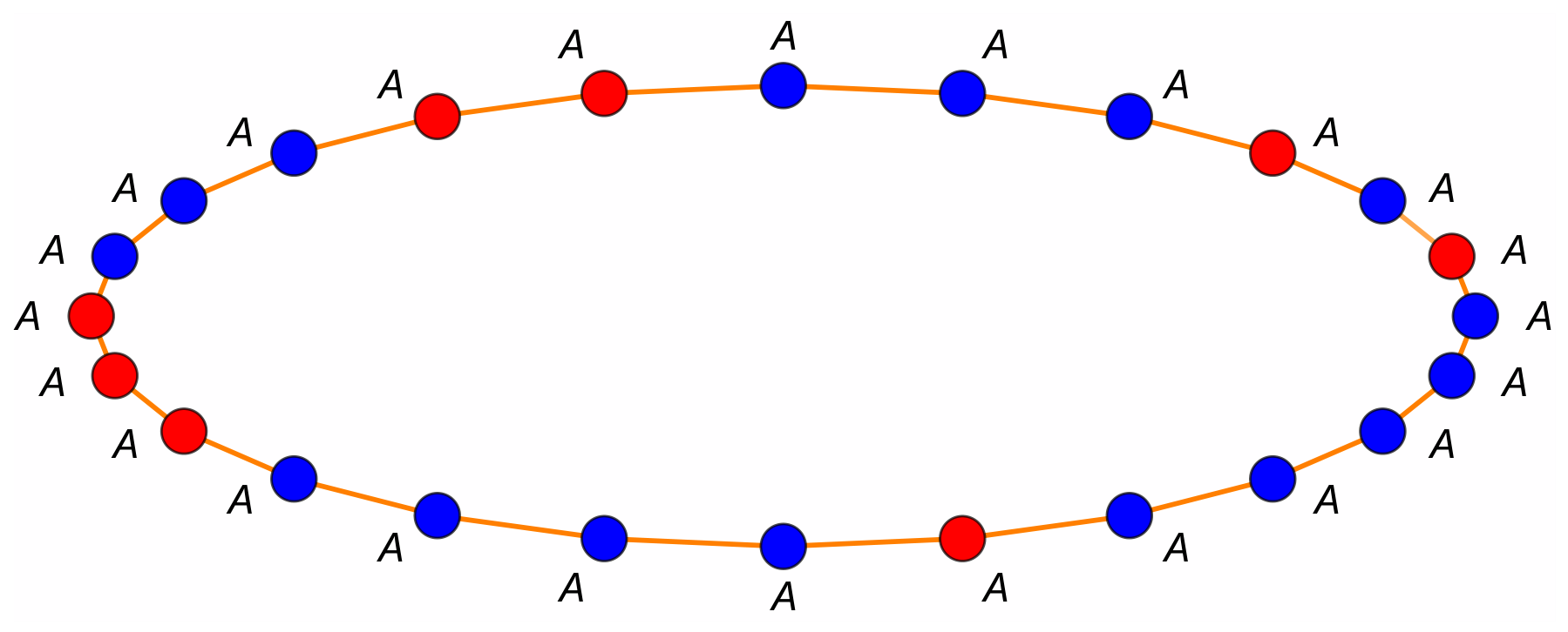
The paper is organized as follows. In Section 2, the corresponding theorems make the above correspondence precise. Section 3 and Section 4 are devoted to the study of the thermodynamic quantities of the Ising model with periodically distributed (p)-site unit cells. These results provide the physical realization of the preceding mathematical framework and are developed for general (p)-site unit cells. Section 5 is devoted to a fluctuation induced well known Casimir force.Section 6 provides a brief overview of the Schottky anomaly, which is subsequently investigated for the models considered in this work. In Section 7, we consider the standard one-dimensional Ising model with periodic boundary conditions ((p=1))the sequence of single letter (AAA…), see Figure 2, uniform interaction coupling (K), and external magnetic field (h), allowing for ferromagnetic ((K>0)) or antiferromagnetic ((K<0)) interactions, as well as positive and negative magnetic fields. In Section 8, we investigate an Ising model with nearest-neighbor interactions modulated by a periodic word of period , namely , over the alphabet , see Figure 5. The model consists of alternating ferromagnetic and antiferromagnetic interactions, and we derive the corresponding free energy in the presence of a constant magnetic field.Finally, Section 9 summarizes the main results and offers some concluding remarks.
2. Algebraic Identities for Matrices in
In what follows, we will need the properties of the general linear group of invertible matrices over the real numbers , i.e. where is the set of all matrices with entries being real numbers. The current section delivers several algebraic identities for matrices . Furthermore, in applications, we are going to consider throughout the paper, we assume that all matrices are entrywise positive. Since the characteristic polynomial of every such matrix has positive discriminant, every matrix considered in this paper has two distinct real eigenvalues. Its determinant can be, however, both positive and negative.
Theorem 1
(Chebyshev representation of matrix powers). Let . For any choice of , define
Let denote the Chebyshev polynomials of the second kind. Then, for all integers ,
where . Moreover, the right-hand side is independent of the choice of the square root of .
Proof.
By the Cayley–Hamilton theorem,
Write
where , , and, by Equation (2),
Assuming that Equation (3) holds for , we obtain
Hence
and therefore
Now define
Since , , and
it follows immediately that
Hence and satisfy the same recurrence with the same initial values, so
Using Equation (4), we derive
Substituting these expressions into Equation (3) yields Equation (1). Finally, using the parity identity
we observe that replacing
changes the factor by , while the argument of the Chebyshev polynomial changes sign, contributing the same factor. These factors cancel in both terms of Equation (1). Hence the right-hand side is independent of the choice of the square root of , completing the proof. □
Remark 1.
The Chebyshev representation avoids explicit diagonalisation and remains valid even when the eigenvalues are complex. As shown in Theorem 2, taking traces immediately yields a closed-form expression for . In transfer-matrix methods of statistical mechanics, where is a positive transfer matrix, the resulting trace formula gives exact finite-size expressions for the partition function.
Theorem 2
(Trace of powers of a matrix). Assume the hypotheses of Theorem 1. Then, for every integer ,
where denotes the Chebyshev polynomials of the first kind.
Proof.
We conclude this section with several remarks highlighting the broad applicability of the mathematical framework developed above to problems in physics. The same algebraic structure has been extensively employed for the special subgroup , consisting of all real matrices with determinant equal to one. This group plays a fundamental role in a wide range of problems in mathematical physics, particularly in the analysis of superlattices, photonic crystals, and more general stratified media.
The use of Chebyshev polynomials in these contexts dates back to the pioneering works of Abelès [6] and Jones [7]. Their subsequent application to transfer-matrix methods and wave-propagation problems has been extensively documented in [8,9,10], as well as in the standard references [11] (§ 1.5.1, p. 69), [12] (§ 1.6.2, p. 55), and the comprehensive reviews [13,14]. In these works, the relevant matrix identities are typically derived using classical techniques, most notably the Cayley–Hamilton theorem, or direct mathematical induction.
In several physical applications, it is advantageous to work with representations of the algebra , which can be naturally extended to the full matrix algebra . The most general formulation of this representation was stated, without proof, in [15]; see also [16], where the associated matrix polynomials are identified with Chebyshev polynomials. These polynomials play a central role in knot theory and arise in a wide variety of mathematical and physical contexts.
The proof presented here applies to an arbitrary invertible matrix and is both elementary and direct. At the formal level, the representation is identical to that for ; the only distinction is that, when , the quantity must be interpreted as a square root in . As established in Theorem 1, the resulting expression is independent of the choice of square root.
3. Ising Model with p Random Variables per Unit Cell
3.1. The Model
Let us consider a chain containing sites labelled by . At each site i we define a discrete random variable
interpreted in physical sciences as a “spin” variable. The mutual dependence of the random variable is determined by interactions constants and bonds , connecting the random variables and .
Let us denote the configuration of the system as
The mutual probability distribution of the N random variables is given by
Explicitly, the Hamiltonian of the system is defined by
depending on the dimensionless parameters
The normalization factor in Equation (7)
is a quantity, used in physical sciences, to define some characteristics of the system of experimental interest, namely—the free energy, specific heat, average value of the random variables (i.e., the magnetisation), and also the Casimir force which is a quantity which study is currently very modern, due to its relation with nanotechnology; definitions of these quantities will be presented below. The parameter has the physical meaning of inverse temperature, where is the Boltzmann constant. We note that the summation in Equation (9) is over all states of the random variables. Different expectation values, e.g., which is called the site magnetisation, are computed with respect to this distribution , namely
Obviously, under periodic boundary conditions does not depend of the positions “i” of the random variable. We will call this, as usual in physical sciences, a magnetisation.
From one derives the so-called free energy of the finite chain, which is of central importance in thermodynamics and statistical physics
as well as the so-called thermodynamics limit of it, defined as
which is connected to the behaviour of the infinite chains (i.e., of the “bulk system”).
3.2. Transfer Matrix Formalism
The transfer-matrix formalism provides a convenient framework for the analysis of the partition function, allowing the free energy and other thermodynamic quantities to be expressed in terms of the eigenvalues of an appropriate transfer matrix.
Throughout this work, we consider Ising chains with periodically modulated couplings of period p, namely
Such periodically modulated Ising chains (with ferromagnetic coupling constants) were introduced and analysed in [4]. Hence, the chain may be regarded as a periodic repetition of a unit cell of length p.
The corresponding local transfer matrices inherit the same periodicity,
where
The transfer matrix associated with one period is therefore
and is commonly referred to as the monodromy matrix, since it describes the evolution of the system over one complete period.
For a chain consisting of n identical unit cells, the total number of sites is . The periodic structure then implies that the transfer matrix of the entire chain is simply the n-th power of the monodromy matrix:
Assuming periodic boundary conditions, the partition function can therefore be written as [4],
Although the monodromy matrix is completely determined by the interaction pattern within a single unit cell, the frustration properties of the corresponding periodic chain depends on the number of repetitions n of that cell. The following proposition provides a precise characterization of the frustration property in the chain.
Proposition 1.
Let
Consider a periodic Ising chain consisting of n repetitions of a unit cell of period p, so that .Then the sign product around the entire ring is
Consequently, the chain is frustrated if and only if
and unfrustrated if and only if
In particular, if
then the chain is unfrustrated precisely when n is even, equivalently,
An immediate consequence of the above proposition is the following corollary, which will be used in Section 8.
Corollary 1.
Consider a periodic Ising chain whose interaction pattern is determined by a repeating unit cell of period p. Assume that the unit cell contains an odd number of antiferromagnetic couplings, i.e.,
Let the total number of spins be , so that the chain consists of m repetitions of the unit cell. Then the chain is unfrustrated if and only if m is even. Equivalently,
We now specialize this result to the interaction patterns considered in the present paper. In particular:
- 1.
-
For the interaction patternwhich has period , the chain is unfrustrated if and only if
- 2.
-
For the interaction patternwhich has period , the chain is unfrustrated if and only if
The above corollary provides a natural classification of the periodically modulated Ising chains studied in this work into frustrated and unfrustrated classes. Since frustration may substantially modify the transfer-matrix spectrum and, consequently, the thermodynamic behavior of the system, these two classes should generally be treated separately when analyzing finite-size effects and thermodynamic properties.
Although is not unimodular in general, its powers admit an exact representation in terms of Chebyshev polynomials after normalization by . As a direct consequence of Theorem 2, we obtain for the partition function:
In what follows, this representation will be systematically exploited for various values of the parameter p.
4. Free Energy Density for General p-Site Unit Cells
Let denote the eigenvalues of the real, nonsingular matrix , ordered so that . From the characteristic equation of , we obtain
Proposition 2.
Since every transfer matrix has strictly positive entries, their product also has strictly positive entries. Writing
with , we obtain
Therefore, the eigenvalues are real and distinct, and the corresponding bulk and finite-size free energies are real-valued, as expected.
Making use of Equation (21), one can calculate the bulk and finite-size free energies, employing the following well-known relations:
Using the above free energies, one obtains:
- the variance of the Hamiltonian in the statistical mechanics is called the specific heat of the system, i.e.,where the averages are taken with respect to the probability distribution Equation (7). It is easy to show thatrespectively for the bulk and finite-size systems. The factor appears because the dominant eigenvalue corresponds to the transfer matrix of a unit cell containing p spins, rather than to a single spin. In the thermodynamic limit the partition function scales asso that the free energy per spin is obtained by dividing by p. Consequently, all thermodynamic quantities defined per spin, including the specific heat, acquire the prefactor .
-
the average values of the random variables, i.e., the magnetisationIt directly follows thatrespectively for the bulk and finite-size systems.
5. Fluctuation-Induced Casimir Force
The fluctuation-induced critical Casimir force arises from finite-size corrections to the free energy, caused by the restriction of thermal fluctuations. It is therefore closely related to the spectral properties of confined systems and serves as a useful probe of finite-size effects. For general introductions and overviews of the subject, see, e.g., Refs. [17,18].
The Casimir force in the one-dimensional Ising model has been extensively investigated in a number of works [19,20,21,22,23]. In the present work, we extend these studies to Ising chains with alternating interactions. Since alternating couplings lead to a nontrivial modification of the energy spectrum, they are expected to produce distinctive features in the corresponding Casimir force.
By definition, we have
Let us first show that, in any of the models outlined above, the free energy density of the finite system approaches exponentially, in n, the corresponding one of the infinite system. From Equation (25) we obtain
where
Since the quantities defined above—the specific heat, the magnetisation and the Casimir force—are expressed via derivates of it follows that they approach their bulk (infinite chain) value exponentially fast when . For the Casimir force we obtain that it itself vanishes exponentially. In statistical physics the quantity is termed the correlation length and describes the rates at which the correlation between the random variables decays with the distance between them.
We close that general chapter by elucidating that the Casimir force is negative, i.e., attractive in physical sciences terminology, independent on the value of p. For establishing that it is enough to perform the explicit calculation of the force using Equation (32). Indeed, one has
The above property holds independent on p and on the choice of values, either positive or negative, of coupling constants . A visualisation of as a function of the scaling variable is presented in Figure 1.
6. Heat Capacity and Schottky Anomaly
The Schottky anomaly is a physical phenomenon characterized by the occurrence of one or more maxima in the temperature dependence of the specific heat. Mathematically, it means that the variance of the sum of the random variables, defining the Hamiltonian of the system, possesses maximum, or maxima, as a function of the parameters characterising the joint probability distribution in the system. It originates from the structure of the energy spectrum and therefore provides useful information about the excitation energies of the system. Since the specific heat vanishes in both the low- and high-temperature limits, it must attain at least one maximum at a finite temperature. For general discussions of the Schottky anomaly, see, e.g., pp. 54–56 of Ref. [25], as well as Refs. [26,27,28].
From a physical perspective, a Schottky peak appears when the thermal energy becomes comparable to the energy gap separating the ground state from a set of excited states. In this temperature range, the occupation probabilities of the corresponding energy levels change most rapidly, leading to enhanced energy fluctuations and, consequently, to a maximum in the specific heat. If several well-separated energy scales are present, the system may exhibit multiple Schottky peaks, each associated with a different excitation gap.
In the present study, the occurrence of a two-peak Schottky anomaly in the one-dimensional Ising model with alternating ferromagnetic and antiferromagnetic interactions () can be understood directly from the spectral decomposition of the transfer matrix. Since the bulk free energy is determined by the logarithm of the dominant eigenvalue, the temperature dependence of thermodynamic quantities is governed by the structure of the transfer-matrix spectrum. When the leading eigenvalue factorizes or contains well-separated characteristic scales, the free energy decomposes into additive contributions associated with distinct excitation gaps. As a consequence, the specific heat exhibits Schottky-type maxima at temperatures determined by these gaps. This spectral interpretation will be made explicit in Sec. Section 8.4.
In what follows we derive exact specific expressions for several Ising type models with p random variables in their unit cell.
7. Ferromagnetic or Antiferromagnetic One-Dimensional Ising Models ()
7.1. On the Case of Negative Determinant
We begin by considering the standard one-dimensional Ising model under periodic boundary conditions with interaction coupling K and external magnetic field h. We consider both the case (), when the mutual influence of two adjacent random variables is positive, i.e., increasing the likelihood the two to have the same values, or the case (), when the opposite is true. In physical sciences the chain with () is called a ferromagnetic one, while () is termed antiferromagnetic.
Figure 2.
Topology of the standard Ising model with identical spins A under periodic boundary conditions. Red (blue) circles denote spins in the state () for the representative configuration shown.
Figure 2.
Topology of the standard Ising model with identical spins A under periodic boundary conditions. Red (blue) circles denote spins in the state () for the representative configuration shown.
These models correspond to the special case , for which reduces to ; see Equation (16). In this case, , with , is the standard transfer matrix of the one-dimensional Ising model. It is a real symmetric matrix with strictly positive entries. Consequently, its eigenvalues , with . The eigenvalues are given by
Hence, Equation (21), together with
gives
Since the determinant of the transfer matrix is negative whenever , at this point the formula Equation (37) is an extension of our previous consideration in refs. [20,29].
Although for , Remark 1 guarantees that the expression in Equation (37) is real and positive and hence
Thus, the partition function remains real and positive even for , despite the fact that the Chebyshev representation formally involves the square root of the negative quantity .
Equations (25) and (28) can be specialized to the present case by setting p = 1, which yields explicit expressions for the free-energy density and the specific heat. As these expressions are straightforward, we do not display them here. Instead, we focus on the corresponding numerical results, which are sufficient to highlight the main physical features of the system, in particular the Schottky anomaly.
7.1.1. Exact Symmetry with Respect to and
Figure 3 shows that, for a periodic chain with an even number of sites N and in the absence of an external magnetic field, the specific heat and the associated Schottky anomaly are identical for ferromagnetic () and antiferromagnetic () interactions, depending only on . In contrast, this symmetry is lost for a periodic chain with an odd number of sites N, as illustrated in Figure 3. This symmetry follows from the staggered spin transformation
which is well defined on a bipartite lattice, such as a one-dimensional periodic chain with an even number of sites, and maps the Hamiltonian with coupling J onto the equivalent Hamiltonian with coupling . Indeed,
so that each nearest-neighbour interaction term changes sign.
Although this transformation acts locally on every bond, its global consistency under periodic boundary conditions, , requires the lattice to be bipartite, which is the case only for even N. For odd N, the lattice is not bipartite, and the staggered transformation Equation (39) cannot be defined consistently around the ring because the bond connecting the last and first sites joins two sites of the same parity. Consequently, the Hamiltonian with coupling J is no longer mapped onto that with coupling . The antiferromagnetic model is therefore geometrically frustrated, and its partition function and thermodynamic properties generally differ from those of the corresponding ferromagnetic model. Hence, for finite periodic chains with an odd number of sites, the free energy, specific heat, and other thermodynamic quantities are not functions of alone.
It is worth noting that the finite-size specific heat in the low-temperature regime, particularly under periodic boundary conditions, was investigated in [30]. The results presented here are fully consistent with those reported therein, thereby providing an independent confirmation of their findings.
7.1.2. Finite-Size Effects
The stronger finite-size effects observed for in Figure 4 originate from the competition between the antiferromagnetic exchange interaction and the external magnetic field. This competition generates low-lying excited states that remain close in energy to the ground state, thereby enhancing the contribution of the subleading eigenvalue of the transfer matrix. As a result, finite-size corrections decay slowly with the system size N, leading to a pronounced size dependence of the specific heat.
By contrast, for the exchange interaction and the magnetic field act cooperatively, resulting in a more robust energy gap and a faster suppression of subleading eigenvalue contributions. Consequently, finite-size corrections decay rapidly with increasing N, and the specific heat becomes only weakly dependent on the system size. This behaviour is reflected in Figure 4, where the finite-size curves quickly collapse onto the bulk result.
In summary, the finite-size behaviour is governed by whether the magnetic field competes with or reinforces the exchange interaction, which determines the effective spectral gap of the transfer matrix and controls the rate of convergence to the thermodynamic limit.
8. Ising Chain of N Sites with Period () Interaction Structure
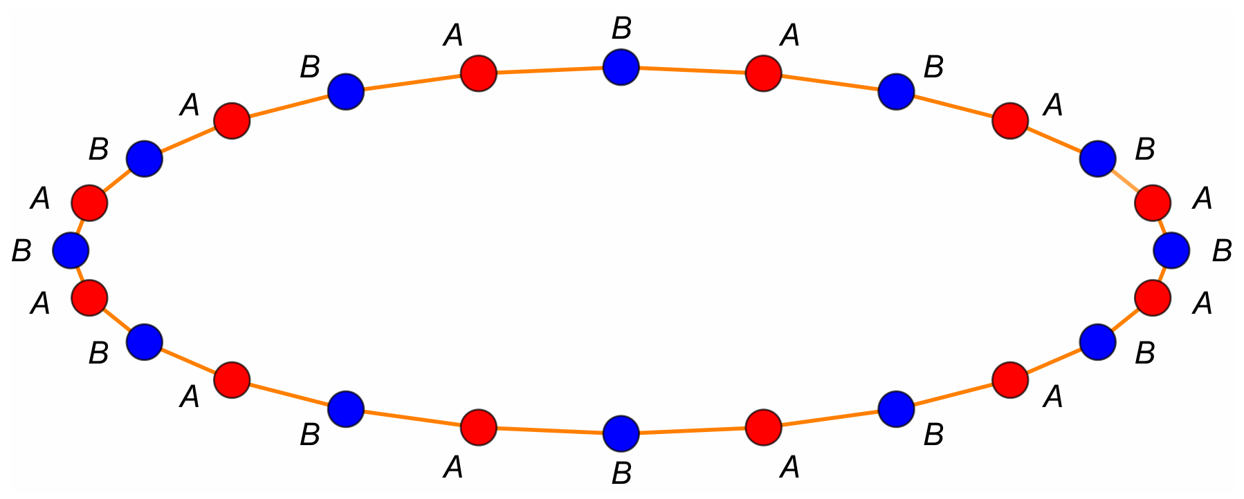
The alternating Ising model with with ferromagnetic coupling constants was first introduced in Ref. [31] and later analyzed in Refs. [32,33,34]. As a prototypical one-dimensional Ising system with spatially modulated exchange interactions, it has served as an important framework for investigating the effects of inhomogeneity and aperiodicity on magnetic properties. In this work we consider the simplest realization of this class, corresponding to spatial period , in our notation. The couplings satisfy Equation (13), thereby defining a two-site unit cell. Each cell contains dynamical variables A and B, with nearest-neighbour interactions and assigned to the bonds and , respectively (see Figure 5).
Figure 5.
Alternating Ising model with two spin species A and B arranged periodically as . The nearest-neighbour couplings and act on the bonds and , respectively.
Figure 5.
Alternating Ising model with two spin species A and B arranged periodically as . The nearest-neighbour couplings and act on the bonds and , respectively.
In the transfer-matrix formalism, we associate the matrices and with the couplings and , respectively and corresponding monodromy matrix:
Periodic boundary conditions require , ensuring an integer number of unit cells and compatibility between lattice periodicity and boundary closure, thus avoiding boundary-induced frustration.
8.1. Thermodynamic Properties
The thermodynamic properties of the system are determined by the eigenvalues of . The matrix explicitly reads
For the above matrix, the eigenvalues are
In the present case,
and
By a straightforward algebraic transformation, the discriminant in Equation (46) can be rewritten as
making it immediately clear that , so that . This also follows from Proposition 2, but the derivation is instructive.
Equations (44) and (45) generalize the results of [32,33], which were obtained in the special ferromagnetic case . The explicit form of the determinant makes the dependence on the signs of and transparent, as it enters through the factors and . In the following, we allow for the more general case .
The dependence on the signs of and is explicit through . Since is an odd function,
the determinant changes sign whenever one coupling changes sign. Therefore:
while
Thus, for nonzero magnetic field , the free energy generally depends on the signs of the couplings, distinguishing ferromagnetic, antiferromagnetic, and mixed ferro–antiferromagnetic configurations.
8.2. Zero-Field Limit
For , Equation (46) yields, after straightforward algebra, the largest eigenvalue
The corresponding zero-field bulk free energy is
Since is an even function, depends only on the absolute values and . In particular, all four combinations , , , and share the same zero-field bulk free energy and the zero-field bulk thermodynamics is invariant under sign reversals of the couplings.
8.3. Specific Heath
The specific heat per spin as defined an Equation (28) the per-spin normalization yields
The temperature dependence of the bulk specific heat , as obtained from Equation (50), is illustrated in Figure 6.
The specific heat thus appears as a superposition of two Schottky-type terms associated with the characteristic energy scales and . When these scales are well separated, , the corresponding activation temperatures are parametrically distinct, leading to two resolved maxima (see: brown, green and black dashed curves in Figure 6) As the interaction strengths become more similar (blue and red curves Figure 6), these maxima progressively coalesce into a single broadened peak.
The double-peak structure therefore directly reflects the coexistence of two distinct energy scales in the transfer-matrix spectrum.
The present model thus provides a minimal realization of a general mechanism: the appearance of multiple Schottky-type maxima as a thermodynamic manifestation of well-separated characteristic energy scales. Similar double-peak structures arise in a variety of systems with hierarchical excitation spectra (see Ref. [26] and references therein).
8.4. On the Emergence of the Double Schottky Structure
The bulk free energy per spin is determined by the dominant eigenvalue of the two-site transfer matrix. For , the largest eigenvalue factorizes, see Equation (49).
Consequently, the bulk free energy becomes additive in the two coupling constants, and the specific heat assumes the exact form
The specific heat is therefore a superposition of two Schottky-type contributions associated with the energy scales and . Each contribution exhibits a maximum at (). When the two energy scales are sufficiently different, the corresponding maxima become well separated, resulting in a characteristic double-peak (double-Schottky) structure. In the special case , the two maxima coincide and merge into a single Schottky peak.
8.5. Frustration and Finite-Size Effects
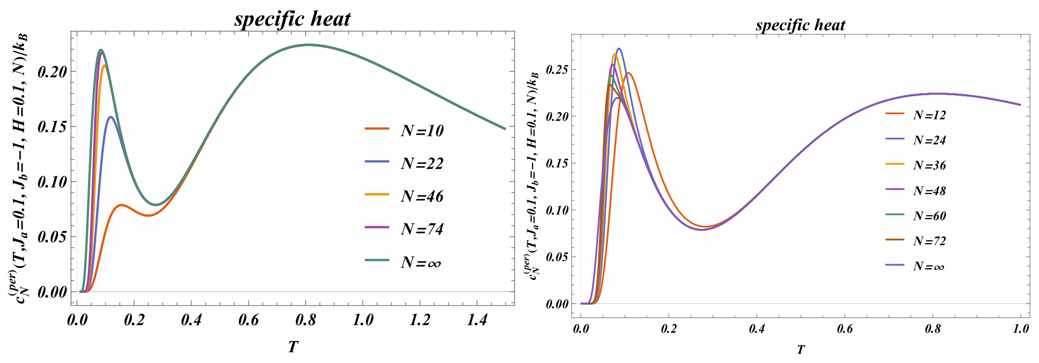
Finite-size effects and frustration in a periodic chain must be analyzed simultaneously, as they are intrinsically intertwined. The finite system size together with the periodic boundary conditions restricts the admissible spin configurations and may modify the manifestation of frustration, while frustration itself can have a significant impact on the finite-size behavior of thermodynamic observables. Consequently, a consistent analysis must treat both effects on an equal footing. Using Equations (28) and (48), this interplay is illustrated in Figure 7, where the system sizes have been chosen in accordance with Corollary 1.
In the thermodynamic limit, the effects of frustration associated with the finite system size vanish, and both the frustrated and unfrustrated finite-size curves converge to the same bulk behavior, as required. The distinction between the two cases is manifested only in the direction of convergence: as shown in Figure 7, one sequence of finite-size curves approaches the bulk curve from above, whereas the other approaches it from below.
9. Summary
The analysis presented in this work relies on Theorems 1 and 2, which express powers and traces of () matrices in terms of Chebyshev polynomials. These results furnish a convenient analytical framework for the study of one-dimensional Ising chains with periodically modulated nearest-neighbour interactions, which constitute the main subject of the present work. The class of models considered here is parametrized by an integer (p), representing the number of interactions within the monodromy matrix and thereby fixing the period of the interaction pattern along the chain. For a chain composed of (n) identical unit cells, the total number of sites is (), and the transfer matrix of the entire system is given by the (n)-th power of the monodromy matrix.
Particular attention has been devoted to the representative cases and . While corresponds to the standard ferromagnetic or antiferromagnetic Ising chain, the case , associated with the interaction pattern ), involve competing ferromagnetic and antiferromagnetic couplings within a single period. Mathematically, if the the interaction is positive (i.e., for a ferromagnetic chain) the adjacent random variables tend to have equal signs (values), while the opposite is true if it is negative (i.e., for an antiferromagnetic chain).
We have performed a detailed study of the double-peak Schottky anomaly in the specific heat. The Schottky anomaly is called an anomaly because the specific heat curve shows a non-intuitive, unexpected peak, or peaks, that does not come from collective critical behaviour, but instead from a very simple microscopic mechanism: a two-level system with an energy gap, or gaps. It looks like a “critical peak”, but it is not reflecting a phase transition(s). That mismatch between appearance and physical origin is why it is historically called an anomaly. Mathematically, it means that the variance of the sum of the random variables, defining the Hamiltonian of the system, possesses maximum, or maxima, as a function of the parameters characterising the joint probability distribution in the system.
Our results confirm that the appearance of two specific-heat maxima is a universal consequence of the presence of two well-separated characteristic energy scales, differing by roughly an order of magnitude, in agreement with previous findings [26]. Unlike earlier investigations, which were largely based on phenomenological multi-level systems, the present work demonstrates in an exact manner the emergence of this phenomenon in a one-dimensional Ising model with competing ferromagnetic and antiferromagnetic interactions subject to an external magnetic field.
One of results of this work is the classification of the models into frustrated and unfrustrated subclasses, according to the parity of the number of unit-cell repetitions. The chain is unfrustrated if and only if and frustrated, otherwise. Consequently, both the and models exhibit frustrated, as well as unfrustrated regimes. They are reflected by nontrivial thermodynamic behaviour and pronounced finite-size effects. We visualised that on the example of the variance of the Hamiltonian of the system, termed specific heat in statistical mechanics, in Figure 3, for , and Figure 7, for . We observe, that the specific heat, for the considered values of the parameters defining the joint probability distribution, possess two maxima as a function of T for . For the specific heat shows one maximum when the sign of interaction is fixed - one for positive, and one for a negative one. The role of the magnetic field in the case is shown in Figure 4. There we see that the finite-size effects depend strongly on the cooperation (), or, in contrast, in competition () between the exchange interaction and the magnetic field.
Finally, let us note that within our approach in terns out to be straightforward to determine the Casimir force within the considered models. Its scaling function is shown in Figure 1. It is remarkable, that this behaviour holds for any set of variables and the magnetisation field h. Note that the behaviour is the same for any p, which a valuable demonstration of the universality [17,24] hypothesis in the theory of critical Casimir force. We note that under periodic boundary conditions the force, as expected, is negative, having the physical meaning of an attraction.
To conclude, let us note that along the lines outlined in the current article, one can consider other, more complicated models, e.e., the case where a ferromagnetic bond of strength is followed by three antiferromagnetic bonds of strength . Repetition of this bond sequence generates a lattice with unit-cell period . A related model was previously investigated in Ref. [35]. That study demonstrated that such a bond arrangement produces a characteristic multi-peak structure in the specific heat as a function of temperature and external magnetic field, as well as a terrace-like structure of the magnetisation. We hope to return to study of such, more complicated systems, in the near future.
Author Contributions
Conceptualization, N.S.T. and D.D.; methodology, N.S.T. and D.D.; software, D.D.; validation, D.D.; formal analysis, N.S.T. and D.D.; investigation, N.S.T. and D.D.; writing—original draft preparation, N.S.T.; writing—review and editing, N.S.T. and D.D.; visualization, D.D. All authors have read and agreed to the published version of this manuscript.
Funding
This work is supported by Grant KP-06-H72/5, competition for financial support for basic research projects—2023, Bulgarian National Science Fund. It was accomplished by the Center of Competence for Mechatronics and Clean Technologies “Mechatronics, Innovation, Robotics, Automation and Clean Technologies”—MIRACle, with the financial support of contract No. BG16RFPR002-1.014-0019-C01, funded by the European Regional Development Fund (ERDF) through the Programme “Research, Innovation and Digitalisation for Smart Transformation” (PRIDST) 2021–2027.
Data Availability Statement
The original contributions presented in this study are included in the article. Further inquiries can be directed to the corresponding author.
Conflicts of Interest
The authors declare no conflicts of interest.
References
- Jagannathan, A. The Fibonacci quasicrystal: Case study of hidden dimensions and multifractality. Rev. Mod. Phys. 2021, 93, 045001. [Google Scholar] [CrossRef]
- Damanik, D.; Embree, M.; Fillman, J. Gap labels for zeros of the partition function of the 1D Ising model via the Schwartzman homomorphism. Indag. Math. 2024, 35, 813–836. [Google Scholar] [CrossRef]
- Baake, M.; Grimm, U.; Joseph, D. Trace maps, invariants, and some of their applications. Int. J. Mod. Phys. B 1993, 7, 1527–1550. [Google Scholar] [CrossRef]
- Barata, J.C.A.; Goldbaum, P.S. On the distribution and gap structure of Lee–Yang zeros for the ising model: Periodic and aperiodic couplings. J. Stat. Phys. 2001, 103, 857–891. [Google Scholar] [CrossRef]
- Yessen, W.N. Properties of 1D classical and quantum Ising models: Rigorous results. Ann. Henri Poincaré 2014, 15, 793–828. [Google Scholar]
- Abelès, F. Recherches sur la propagation des ondes électromagnétiques sinusoïdales dans les milieux stratifiés. Applications aux couches minces English title: “Research on the propagation of sinusoidal electromagnetic waves in stratified media. Applications to thin films”. Ann. Phys. 1950, 12, 596–640 and 706–782. [Google Scholar] [CrossRef]
- Jones, H. The electron energy spectrum in long period superlattices. J. Phys. F. Met. Phys. 1973, 3, 2075–2085. [Google Scholar] [CrossRef]
- Sprung, D.W.L.; Wu, H.; Martorell, J. Scattering by a finite periodic potential. Am. J. Phys. 1993, 61, 1118–1123. [Google Scholar] [CrossRef]
- Wu, H.; Sprung, D.W.L.; Martorell, J. Periodic quantum wires and their quasi-one dimensional nature. J. Phys. D. Appl. Phys. 1993, 26, 798–803. [Google Scholar] [CrossRef]
- Griffiths, D.J.; Steinke, C.A. Waves in locally periodic media. Am. J. Phys. 2001, 69, 137–154. [Google Scholar] [CrossRef]
- Furman, S.A.; Tikhonravov, A.V. Basics of Optics of Multilayer Systems; Atlantica Séguier Frontieres; World Scientific Publishing Co., Pte. Ltd.: Singapore, 1992. [Google Scholar]
- Born, M.; Wolf, E. Principles of Optics: Electromagnetic Theory of Propagation, Interference and Diffraction of Light, chapter 1.6. In Theory of Dielectric Films, 7th ed.; Cambridge University Press: Cambridge, UK, 1999; pp. 54–65. [Google Scholar]
- Sánchez-Soto, L.L.; Monzón, J.J.; Barriuso, A.G.; Cariñena, J.F. The transfer matrix: A geometrical perspective. Phys. Rep. 2012, 513, 191–227. [Google Scholar] [CrossRef]
- Pereyra, P. The transfer matrix method and the theory of finite periodic systems. From heterostructures to superlattices. Phys. Status Solidi B 2022, 259, 2100405. [Google Scholar]
- Brandi, R.; Ricci, P.E. Composition Identities of Chebyshev Polynomials via 2×2 Matrix Powers. Symmetry 2020, 12, 746. [Google Scholar] [CrossRef]
- Owczarek, R. Remarks on Chebyshev polynomials, Fibonacci polynomials and Kauffman bracket skein modules. J. Knot Theor. Ramif. 2018, 27, 1841007. [Google Scholar] [CrossRef]
- Dantchev, D.M.; Dietrich, S. Critical Casimir effect: Exact results. Phys. Rep. 2023, 1005, 1–130. [Google Scholar] [CrossRef]
- Dantchev, D. On Casimir and Helmholtz fluctuation-induced forces in micro-and nano-systems: Survey of some basic results. Entropy 2024, 26, 499. [Google Scholar] [CrossRef] [PubMed]
- Rudnick, J.; Zandi, R.; Shackell, A.; Abraham, D. Boundary conditions and the critical Casimir force on an Ising model film: Exact results in one and two dimensions. Phys. Rev. E 2010, 82, 041118. [Google Scholar] [CrossRef] [PubMed]
- Dantchev, D.M.; Tonchev, N.S.; Rudnick, J. Casimir versus Helmholtz forces: Exact results. Ann. Phys. 2023, 459, 169533. [Google Scholar] [CrossRef]
- Dantchev, D.M.; Tonchev, N.; Rudnick, J. Casimir and Helmholtz forces in one-dimensional Ising model with Dirichlet (free) boundary conditions. Ann. Phys. 2024, 464, 169647. [Google Scholar] [CrossRef]
- Dantchev, D.; Tonchev, N.; Rudnick, J. Finite-size Nagle-Kardar model: Casimir force. Phys. Rev. E 2024, 110, L062104. [Google Scholar] [CrossRef] [PubMed]
- Dantchev, D.; Tonchev, N. A Brief Survey of Fluctuation-Induced Interactions in Micro and Nano-Systems and One Exactly Solvable Model as Example. In Advanced Computing in Industrial Mathematics. BGSIAM 2023; Lilkova, E., Datcheva, M., Aleksandrova, T., Eds.; Studies in Computational Intelligence; Springer: Cham, Switzerland, 2025; Volume 1219, pp. 44–58. [Google Scholar] [CrossRef]
- Brankov, J.G.; Dantchev, D.M.; Tonchev, N.S. The Theory of Critical Phenomena in Finite-Size Systems—Scaling and Quantum Effects; World Scientific: Singapore, 2000. [Google Scholar]
- Mussardo, G. An Introduction to Exactly Solved Models in Statistical Physics Statistical Field Theory, 2010.
- Souza, M.d.; Paupitz, R.; Seridonio, A.; Lagos, R.E. Specific heat anomalies in solids described by a multilevel model. Braz. J. Phys. 2016, 46, 206–212. [Google Scholar] [CrossRef]
- Akiyama, H.; Jido, D. Systematic study of hadronic excitation energy using the Schottky anomaly. Phys. Rev. D. 2021, 104, 114014. [Google Scholar] [CrossRef]
- Tonchev, N.S.; Dantchev, D. Chebyshev Polynomials in the Physics of the One-Dimensional Finite-Size Ising Model: An Alternative View and Some New Results. Condens. Matter 2024, 9, 53. [Google Scholar] [CrossRef]
- Tonchev, N.S.; Dantchev, D. The Algebra of Chebyshev Polynomials and the Transfer-Matrix Approach for the One-Dimensional Ising Model with a Defect. Mathematics 2026, 14, 741. [Google Scholar] [CrossRef]
- Lee, J. Low-temperature behavior of the finite-size one-dimensional Ising model and the partition function zeros. J. Korean Phys. Soc. 2014, 65, 676–683. [Google Scholar] [CrossRef]
- Lu, J.P.; Odagaki, T.; Birman, J.L. Properties of one-dimensional quasilattices. Phys. Rev. B 1986, 33, 4809. [Google Scholar] [CrossRef]
- Grimm, U.; Baake, M. Aperiodic Ising Models. arXiv 1996, arXiv:cond-mat/9604116. [Google Scholar]
- Baake, M.; Grimm, U. Aperiodic order and quasicrystals. In The Mathematics of Long-Range Aperiodic Order; Moody, R.V., Ed.; NATO ASI Series C: Mathematical and Physical Sciences; Springer: Dordrecht, The Netherlands, 1997; Volume 489, pp. 197–237. [Google Scholar]
- Baake, M.; Grimm, U. Aperiodic Order; Cambridge University Press: Cambridge, UK, 2013; Volume 1. [Google Scholar]
- Doman, B.; Williams, J. Fibonacci and Lucas polynomials. In Proceedings of the Mathematical Proceedings of the Cambridge Philosophical Society; Cambridge University Press: Cambridge, UK, 1981; Volume 90, pp. 385–387. [Google Scholar]
Figure 1.
The behaviour of the scaling function of the Casimir force as a function of . This behaviour holds for any set of variables and the magnetisation field h. Note that the behaviour is the same for any p, which a valuable demonstration of the universality [17,24] hypothesis in the theory of critical Casimir force.
Figure 1.
The behaviour of the scaling function of the Casimir force as a function of . This behaviour holds for any set of variables and the magnetisation field h. Note that the behaviour is the same for any p, which a valuable demonstration of the universality [17,24] hypothesis in the theory of critical Casimir force.
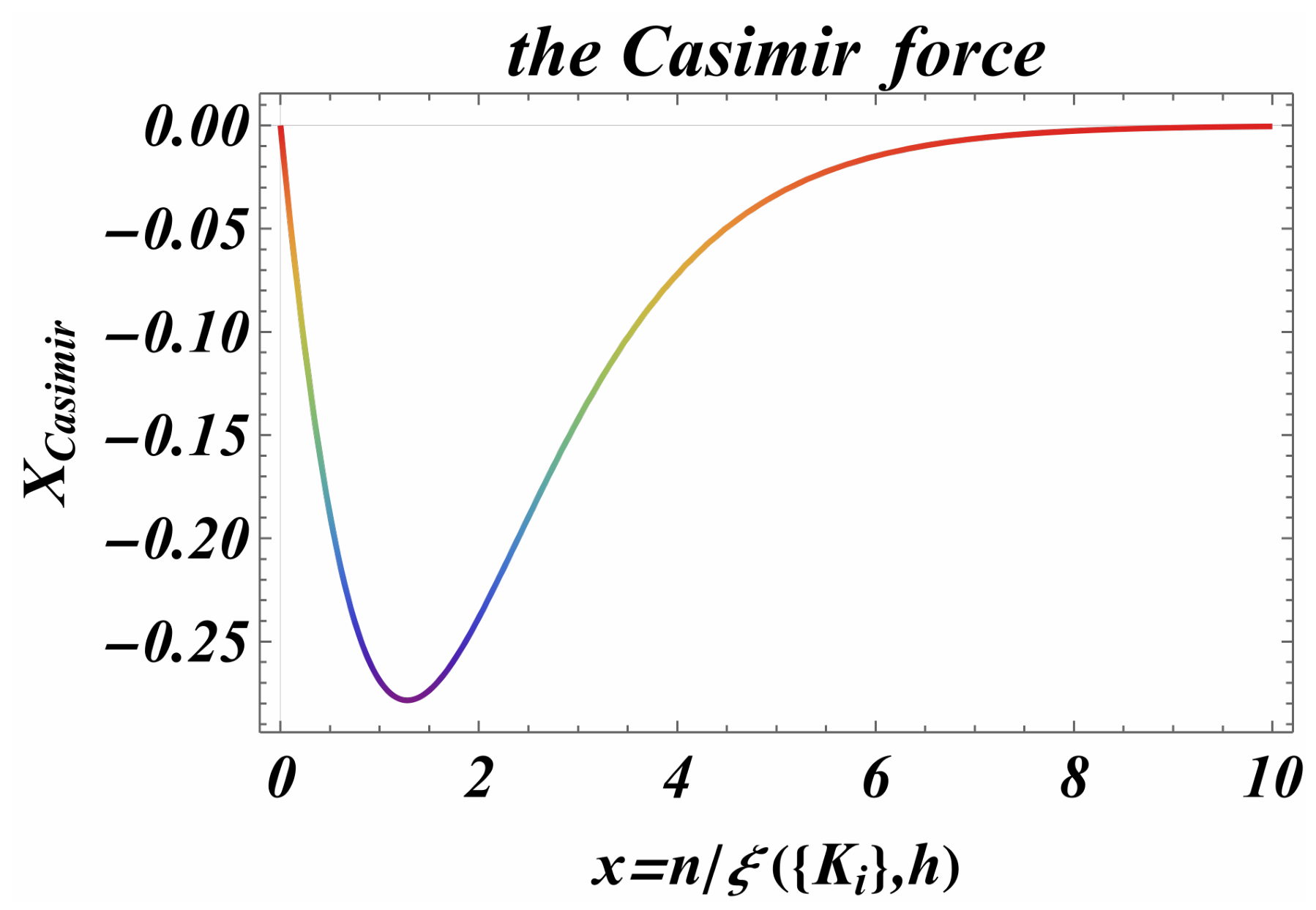
Figure 3.
The finite-size specific heat of the Ising model in the absence of the magnetic fields for different numbers N (left) for even number of random variables as a function of for the antiferromagnetic interaction (the left side of the figure) and ferromagnetic interaction (the right of the figure). (right) The same, but for odd numbers of random variables.
Figure 3.
The finite-size specific heat of the Ising model in the absence of the magnetic fields for different numbers N (left) for even number of random variables as a function of for the antiferromagnetic interaction (the left side of the figure) and ferromagnetic interaction (the right of the figure). (right) The same, but for odd numbers of random variables.
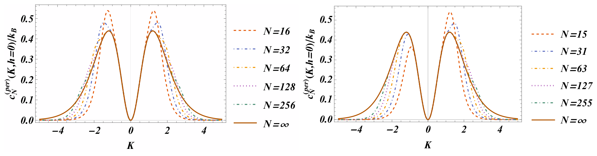
Figure 4.
Finite-size specific heat of the Ising model in a magnetic field for different system sizes, shown as a function of . The left panel corresponds to the antiferromagnetic case , while the right panel corresponds to the ferromagnetic case .
Figure 4.
Finite-size specific heat of the Ising model in a magnetic field for different system sizes, shown as a function of . The left panel corresponds to the antiferromagnetic case , while the right panel corresponds to the ferromagnetic case .
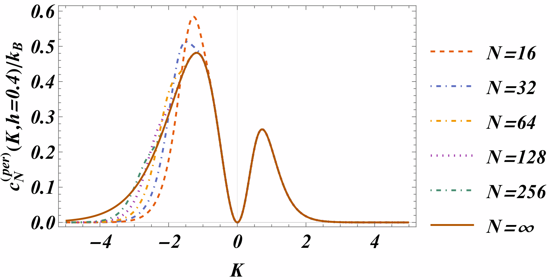
Figure 6.
Bulk specific heat versus temperature T for the model, for several combinations of the ferromagnetic interaction and antiferromagnetic interaction and magnetic field .
Figure 6.
Bulk specific heat versus temperature T for the model, for several combinations of the ferromagnetic interaction and antiferromagnetic interaction and magnetic field .
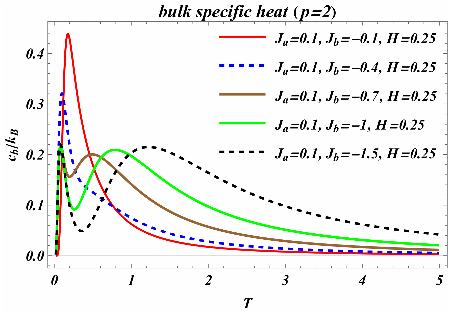
Figure 7.
Specific heat as a function of the temperature T for the model with and with a magnetic field . (left) The various system sizes N considered in the figure satisfy corresponding to the condition for a frustrated chain. (right) Specific heat , as a function of temperature T for the model, for values of and , that differ substantially in magnitude.The various system sizes N considered in the figure satisfy corresponding to the condition for unfrustrated chain.
Figure 7.
Specific heat as a function of the temperature T for the model with and with a magnetic field . (left) The various system sizes N considered in the figure satisfy corresponding to the condition for a frustrated chain. (right) Specific heat , as a function of temperature T for the model, for values of and , that differ substantially in magnitude.The various system sizes N considered in the figure satisfy corresponding to the condition for unfrustrated chain.
Disclaimer/Publisher’s Note: The statements, opinions and data contained in all publications are solely those of the individual author(s) and contributor(s) and not of MDPI and/or the editor(s). MDPI and/or the editor(s) disclaim responsibility for any injury to people or property resulting from any ideas, methods, instructions or products referred to in the content. |
© 2026 by the authors. Licensee MDPI, Basel, Switzerland. This article is an open access article distributed under the terms and conditions of the Creative Commons Attribution (CC BY) license (http://creativecommons.org/licenses/by/4.0/).
Copyright: This open access article is published under a Creative Commons CC BY 4.0 license, which permit the free download, distribution, and reuse, provided that the author and preprint are cited in any reuse.