

Submitted:
09 July 2026
Posted:
10 July 2026
You are already at the latest version
Abstract
Remote swell generated far from land can deliver hazardous wave energy to island coasts many tens of hours after the responsible wind event has ceased locally. Forecasting this hazard typically relies on full spectral wave models forced by global winds, which require specialized input data, computational infrastructure and expert interpretation. Here we present a reduced physical framework that constrains the amplitude envelope of long-range swell along a single dominant ray, using deep-water dispersion, steepness-limited saturation and post-source attenuation. The reduced model describes three successive regimes. First, remote wind input increases the significant wave height Hs from approximately 3 m to a physically derived saturation level of about 5.8 m. Second, Hs reaches a quasi-steady plateau when the bulk steepness ε=kHs/2 approaches a threshold εth≈0.06, so that whitecapping dissipation balances further wind-driven growth. Third, after leaving the forcing region, the swell decays slowly during propagation and can still arrive offshore with Hs of order 4 m after approximately 72 h. For a representative 14 s swell packet, this corresponds to a deep-water group velocity of about 10.9 m s-1, a travel distance of about 2830 km, and an effective attenuation length of about 7500 km. The analytical envelope is tested against quality-controlled measurements from the Graciosa buoy, Azores, in the North Atlantic. In the analysed record, 117 observations satisfied Hs≥4 m and 12≤Tp≤16 s. The strongest selected long-period candidate reached Hs=5.98 m with Tp=15.4 s, remaining below the corresponding steepness-limited ceiling for εth=0.06. The buoy data support the proposed envelope as a physically grounded reference for energetic long-period swell near the Azores. The framework provides an interpretable first-alert diagnostic for assessing whether a remote swell packet is capable of producing hazardous offshore conditions at Azorean island coasts, while remaining complementary to full spectral wave forecasting.
Keywords:
remote swell
; long-period waves
; Azorean island coasts
; coastal wave hazard
; steepness-limited saturation
; whitecapping dissipation
; significant wave height
; deep-water wave propagation
; upper-bound envelope
; buoy measurements
1. Introduction
Long-period swell generated by remote storms can impact island coasts days after the local winds have calmed. Measurements in both the Atlantic and Pacific show that energetic swell packets produced by intense storm systems can propagate thousands of kilometres across deep water and still arrive with metre-scale significant wave heights , well after the generating winds have ceased at the target location. Classic basin-scale tracking demonstrated that swell originating in one part of an ocean basin can cross essentially the entire basin and remain hazardous on arrival [1]. This basin-scale persistence has since been confirmed by satellite and modelling studies, which show that swell systems can retain a coherent spectral identity over several days of propagation and across ocean-basin distances [2,3,4,5]. This is a direct operational problem for isolated archipelagos, including mid-Atlantic islands such as the Azores: port operations, coastal safety and nearshore infrastructure can all be affected by 3–4 m offshore swell even under otherwise calm local weather.
At present, forecasting of remote-swell arrival is handled mainly by third-generation spectral wave models such as WAVEWATCH III–class systems. These models solve the spectral wave-action balance for the full two-dimensional wave spectrum under wind forcing, including wind input, nonlinear wave–wave transfers, and dissipation by whitecapping and breaking [6,7]. They can provide global fields of significant wave height, peak period and direction, often with several days of lead time. In operational and research practice, these models are increasingly combined with satellite products — SAR wave mode, Sentinel-1A/B, wide-swath altimetry, CFOSAT, SWOT and related directional wave measurements — to improve the description of swell amplitude and direction across basins and to validate forecasts against real propagation events [5,8,9,10,11,12,13].
However, these products are not automatically translated into a compact physical envelope for island-scale hazard interpretation. Full spectral models provide technically rich outputs, including directional spectra, multiple wave partitions and source diagnostics, but they do not usually express the result as a simple amplitude ceiling such as: what is the largest offshore swell height that can plausibly survive a multi-day propagation path toward an island? This distinction is important for small island settings, where the immediate operational question is often whether a remote event can produce hazardous offshore swell within the next 2–4 days.
The literature on long-range swell propagation provides two constraints that are central to the present framework. First, long-period swell in deep water can propagate with weak attenuation, with e-folding scales of several thousand kilometres and, in low-steepness cases, even more than 10,000–20,000 km [2,3,4]. Second, swell dissipation increases strongly with steepness. Satellite SAR and in situ data show that steeper swell loses energy faster, while low-steepness swell can travel over basin scales with comparatively weak decay [2,3]. Independent breaking-probability and whitecapping studies also show that dominant-wave breaking is strongly linked to wave steepness and spectral saturation [14,15,16,17]. These results suggest a physically controlled amplitude ceiling: once a swell packet becomes too steep, enhanced whitecapping and active breaking prevent indefinite growth.
This steepness-controlled ceiling is already implicit in whitecapping source terms. Operational wave models use source-term formulations that trigger enhanced dissipation when the wave field exceeds nonlinear thresholds such as crest slope, spectral saturation or steepness-related criteria, and they treat that dissipation as a dominant sink balancing wind input once waves become highly energetic [14,15,16,17,18]. The mechanism itself is therefore not new. What is less commonly available is a reduced, transparent formulation that converts this internal dissipation physics into an interpretable upper-bound envelope for island-scale swell hazard.
A further complication is that measured sea states are rarely pure single-component swell systems. They often contain wind sea, one or more swell partitions and mixed directional components. Recent CFOSAT-based sea-state classification studies highlight the importance of separating swell-dominated states from mixed or wind-sea-dominated conditions when interpreting wave records [12]. This is particularly relevant for island settings: a high value alone is not sufficient to identify a long-range swell hazard unless the associated peak period and steepness are also considered.
What is missing is therefore a compact, first-order formulation that:(i) states explicitly that steepness-triggered whitecapping can act as a physical growth limiter, setting an offshore saturation level for significant wave height under strong remote forcing;(ii) separates this saturation height, controlled mainly by and , from the arrival height, controlled mainly by post-source attenuation; and(iii) converts this physical picture into a practical upper-bound envelope that can be checked against local island-scale measurements.
Reduced physical envelopes of this type are most useful when tested against real wave measurements. For the Azores, quality-controlled buoy records provide a direct way to assess whether energetic long-period sea states remain below, or approach, the steepness-limited ceiling predicted by the reduced model [19]. This use of in situ buoy data complements satellite-based approaches: satellite missions provide basin-scale coverage and directional information, while buoy records provide direct local measurements of , and wave direction at the island scale [5,8,9,10,11,12,20,21].
In this work, we address this gap by proposing and analysing a reduced swell-evolution framework for long-range island hazard assessment and by testing its implications against measurements from the Graciosa buoy, Azores [19]. The study has five main components:
(1) Bulk energy balance for a single swell packet. We collapse the full spectral wave-action balance into an ordinary differential equation for the significant wave height of the dominant swell component along its propagation path. The retained processes are remote wind input, steepness-dependent whitecapping dissipation and weak propagation-related losses after the packet leaves the source region [6,7,18].
(2) Steepness-limited saturation as a dynamical ceiling. We show that the swell saturates when its bulk steepness approaches a threshold , taken here within the representative range for energetic long-period swell in deep water. For the reference case and , this gives [14,15,16,17,18].
(3) Slow decay and multi-day survival. Once the packet exits the forcing region, direct wind input vanishes and the swell decays more slowly. In the reference case, a 14 s swell packet travels approximately 2830 km in 72 h, and a decay from to corresponds to an effective attenuation length of approximately 7500 km [1,2,3,4,5].
(4) A practical upper-bound hazard diagnostic. The framework converts steepness-limited saturation and post-source decay into a physically interpretable first-alert envelope. Its purpose is not to replace full spectral forecasting, but to estimate whether a remote swell packet is physically capable of producing hazardous offshore conditions at an island coast.
(5) Test using Graciosa buoy measurements. We use quality-controlled Graciosa buoy records to test whether energetic long-period sea states observed near the Azores are consistent with the proposed envelope [19]. In the analysed record, 117 observations satisfy and . The strongest selected long-period candidate reaches with , remaining below the predicted reference steepness-limited ceiling for .
The contribution of this study is therefore a physically constrained upper-bound framework tested against Graciosa buoy measurements, not a deterministic replacement for spectral wave forecasting. It identifies steepness-limited saturation as the mechanism that caps swell growth under remote forcing, explains how part of that capped amplitude can survive multi-day propagation, and recasts these processes as an interpretable diagnostic for long-range swell hazard at Azorean island coasts. This study follows a physics-based approach in which dispersion, nonlinear steepness limitation and attenuation are used as reduced descriptors of a complex oceanographic process.
2. Materials and Methods
2.1. Reduced Physical Description of the Swell Packet
We consider a coherent long-period swell packet generated in a remote wind-forced region and subsequently propagating across deep water toward an island coast. The packet is described by a dominant peak period , a corresponding deep-water wavenumber , and a bulk significant wave height along its propagation path.
The purpose of the present framework is not to reproduce the full directional wave spectrum. Instead, the spectral wave-action balance is reduced to a one-dimensional envelope model for the dominant swell component. This reduction retains only the leading-order processes that control the packet amplitude: wind input during remote generation, steepness-controlled whitecapping dissipation, and weak propagation-related losses after the packet leaves the forcing region.
The reduced approach is motivated by the same physical structure used in third-generation spectral wave models, but with a different objective. Full models resolve the spectral wave-action balance, source terms and propagation over space, frequency and direction [6,7], whereas the present framework extracts only the amplitude-limiting physics needed to define a transparent saturation envelope.
The starting point is the spectral wave-action balance,
where is the wave-action density, is the intrinsic radian frequency, is the group-velocity vector, and is the total source/sink term. In third-generation wave models,
where is wind input, represents nonlinear wave–wave interactions, and represents dissipation, dominated here by whitecapping and breaking [6,7,18].
For the present reduced model, this full spectral balance is projected onto one dominant swell component centred on . The result is a ray-following amplitude model. The model does not claim to predict the exact value of at every time along the trajectory. Rather, it constrains the amplitude scale through three physical quantities: the group velocity, the steepness threshold and the attenuation length.
The Graciosa buoy measurements are therefore used as a local test of the envelope, not as a calibration of all source terms. The buoy data test whether energetic long-period sea states observed near the Azores remain within the steepness-limited bounds predicted by the reduced model [19].
2.2. Bulk Energy Equation
For a narrow-band deep-water swell component, the bulk wave-energy density scales with the square of the significant wave height and can be expressed as
where is a constant that depends on the precise wave-height convention used. The value of this constant is not essential for the present framework, because the saturation height is derived from a nondimensional steepness threshold instead of from an absolute calibration of the energy source terms.
Along the dominant ray, the reduced energy budget may be written as
where is the effective wind-energy input into the dominant swell component, is dissipation by whitecapping and active breaking, and represents propagation-related losses, including geometric spreading and weak nonlinear leakage away from the dominant component.
Since , the amplitude evolution can be expressed in terms of relative growth and decay rates:
where is the effective wind-input growth rate, is the steepness-dependent whitecapping decay rate, and is the weak propagation/spreading decay rate.
This rate-based formulation avoids introducing an unnecessary calibration of the absolute source terms. The physical conclusions depend on the relative balance between input and dissipation, and on the steepness condition, not on the numerical prefactor used in the bulk energy definition.
The three regimes may therefore be written compactly as:
During the growth regime, wind input exceeds the combined loss terms and increases. During saturation, steepness-dependent whitecapping balances wind input. During free propagation, direct wind input vanishes and the packet decays slowly under residual propagation losses.
The key point is that the saturation condition is controlled by the bulk steepness,
rather than by the absolute normalisation of the energy equation. This is why the saturation height can be derived directly from the threshold condition , as shown below.
This rate-based representation is consistent with recent source-term developments in which dissipation is made strongly dependent on breaking probability, spectral saturation or steepness-related quantities [14,15,16,17,18]. The reduced model does not reproduce those source terms in detail; instead, it retains their common physical implication: once the wave field becomes sufficiently steep, dissipation increases rapidly and limits further amplitude growth.
2.3. Deep-Water Dispersion and Travel-Time Scale
For deep-water gravity waves,
The phase velocity and group velocity are therefore
Using , the deep-water wavenumber is
and the group velocity becomes
For the representative long-period swell considered in this study, . This gives
And
Over a 72 h propagation time, the corresponding propagation distance is approximately
This calculation fixes the space–time scale of the problem. A 14 s swell packet naturally travels a few thousand kilometres in approximately three days. Therefore, the 72 h warning time used in this framework follows directly from deep-water dispersion and is not an arbitrary operational assumption.
This group-velocity scale is consistent with classic basin-scale swell tracking and with modelling studies of long-range propagation. Snodgrass et al. showed that swell energy can remain coherent over ocean-basin distances, while numerical and satellite-based studies confirm that long-period swell can be followed over multi-day, multi-thousand-kilometre paths [1,2,3,4,5].
The same dispersion relation also provides the wavenumber used in the steepness calculation. This is important for internal consistency: the travel-time scale, the saturation height and the steepness diagnostic are all derived from the same peak period , instead of being chosen independently.
For each Graciosa buoy record, the observed determines both the wavenumber used in Equation (6) and the corresponding saturation ceiling . The comparison with the buoy data is therefore period-dependent, rather than based on a single fixed wave-height threshold.
2.4. Wave Steepness and Whitecapping Threshold
The nonlinear state of the dominant swell component is described using the bulk steepness defined in Equation (6). This variable links the amplitude of the packet to its tendency to undergo active breaking and whitecapping. Studies of swell dissipation show that attenuation depends strongly on steepness: low-steepness swell can propagate over very long distances, whereas steeper swell dissipates much more rapidly [2,3]. The use of steepness as a bulk diagnostic is also supported by studies of breaking probability and whitecapping. Dominant-wave breaking has been shown to depend strongly on wave steepness and spectral saturation, and recent source-term formulations increasingly treat whitecapping as a nonlinear response to saturation or breaking-related thresholds [14,15,16,17,18].
We assume that efficient whitecapping becomes dynamically important when
where is a practical threshold for breaking-dominated dissipation. For energetic long-period swell in deep water, a representative range is
In the reference calculation, we use . This threshold is not treated as a universal constant. It is a practical bulk criterion representing the onset of efficient whitecapping in the dominant swell component. The sensitivity analysis therefore explores the range , instead of relying only on the reference value. This qualification is particularly relevant when interpreting the Graciosa buoy measurements. Real buoy records may include mixed wind-sea and swell components, and recent global sea-state classifications based on CFOSAT observations demonstrate that separating swell-dominated states from mixed conditions is essential when interpreting , and wave direction [12]. For this reason, the Graciosa analysis focuses specifically on energetic long-period records, rather than treating every high- sea state as a clean remote-swell event.
2.5. Steepness-Limited Saturation Height
The main mechanism of the framework is steepness-limited saturation. During the growth stage, increases the energy of the swell packet. However, as increases, the steepness also increases. Once approaches , whitecapping dissipation becomes strong enough to balance further wind-driven growth. In the rate-based notation introduced above, this saturation condition is written as
This formulation is consistent with whitecapping and dissipation source-term developments, in which breaking and dissipation increase nonlinearly with steepness, spectral saturation or breaking probability instead of acting as a constant background loss [14,15,16,17,18]. When this balance is reached, the bulk amplitude no longer increases appreciably, so that
The swell packet then reaches a quasi-steady saturation height. Since , the threshold condition gives
Substituting Equation (9) into Equation (12) yields
For and ,
This value is important for the reference case. The saturation height is not a fitted or imposed plateau. It follows directly from the combination of the deep-water dispersion relation and a physically meaningful steepness threshold for active whitecapping.
The key point is that the amplitude ceiling is obtained before any comparison with the buoy data. The Graciosa measurements are therefore not used to tune ; they are used later to test whether observed energetic long-period sea states remain compatible with the steepness-limited envelope.
The scaling
is especially important. It means that long-period swell can sustain a much larger bulk height before reaching the same steepness threshold. Conversely, short-period swell reaches the breaking-controlled ceiling at a lower significant wave height. This scaling is the physical reason why long-period swell is particularly relevant for island hazard: it is both fast enough to cross basin-scale distances in a few days and capable of carrying metre-scale amplitude after saturation.
This period dependence is also important when projecting the Graciosa buoy measurements onto the saturation envelope. A single value such as applies only to the reference case . For the Graciosa buoy records, the appropriate saturation ceiling must be evaluated using the observed of each sea state. This is why the later -versus- comparison is a stronger test of the model than comparison with a single fixed wave-height threshold.
2.6. Post-Saturation Decay and Effective Attenuation Length
After the swell packet leaves the remote forcing region, direct wind input into the dominant component vanishes:
The reduced rate equation then becomes
Because the packet is no longer being actively forced, its steepness relaxes slightly. Since is a strongly nonlinear function of , this reduction in steepness weakens whitecapping substantially. The remaining decay is then dominated by slower propagation-related losses.
This behaviour is consistent with swell-dissipation studies showing that attenuation depends strongly on steepness: low-steepness swell can propagate across very long distances with weak decay, whereas steeper swell dissipates more rapidly [2,3]. Long-range modelling studies also show that basin-scale swell decay can be represented through effective attenuation behaviour, although the underlying mechanisms remain distributed across several processes [4].
In the reduced envelope model, these post-source losses are represented by an effective attenuation length . This parameter does not describe a single dissipation mechanism. Instead, it summarises the combined effect of directional spreading, weak nonlinear leakage, residual whitecapping and any unresolved propagation losses along the dominant ray.
This post-source decay is represented as
For the reference case, the propagation distance is
If the packet arrives with from a saturation height , then the required effective attenuation length is
Substituting the representative values gives
Thus, an arrival height of approximately 4 m is consistent with an effective swell attenuation length of order
This value lies within the broad observed range for long-period swell attenuation, particularly after the packet has relaxed below the strongest breaking regime [2,3,4].
The attenuation length is the main uncertainty in the arrival estimate. For this reason, the model does not present as a single deterministic forecast. Instead, is treated as a sensitivity parameter controlling how much of the saturated amplitude survives the propagation. The saturation height is fixed primarily by steepness and period; the arrival height is determined by attenuation during propagation. This separation is fundamental to the logic of the reduced model.
This distinction is also important when comparing the envelope with Graciosa buoy measurements. Buoy records near the Azores are not expected to reproduce exactly the reference value . Instead, they are used to test whether observed energetic long-period sea states remain compatible with the steepness-limited envelope and with plausible attenuation from a remote source region.
2.7. Reduced Closure in Terms of Characteristic Rates
The reduced amplitude equation, Equation (5), can also be interpreted in terms of characteristic growth and decay rates. In this notation, the three regimes correspond to growth, saturation and free propagation, as described in Section 2.2.
A generic threshold-like representation of whitecapping is
This expression is not used as a calibrated source term. Its role is to encode the required physical behaviour: whitecapping is weak below the threshold and increases rapidly once exceeds . The exact values of and are therefore not needed to derive the saturation height, because the ceiling follows from the threshold condition itself.
This closure is deliberately minimal, but it is physically aligned with more detailed source-term formulations. Although explicit breaking-probability approaches and saturation-based whitecapping formulations differ in implementation, they share the qualitative behaviour required here: dissipation remains limited below a threshold and increases sharply once the sea state becomes sufficiently steep or saturated [14,15,16,17,18].
The propagation decay rate can be related to the attenuation length through
This closes the reduced interpretation: fixes and , fixes , and fixes the residual amplitude at landfall. These three quantities form the minimal physical basis of the saturation envelope.
This closure also clarifies how the Graciosa buoy measurements are used in the framework. The buoy data are not used to calibrate , , , or . Instead, they are used to test whether observed energetic long-period sea states fall within the steepness-limited envelope implied by , , and .
This point is important because real sea states may contain multiple partitions. The reduced framework is intended for sea states with a dominant long-period component, identified through . For this reason, the later filtering step excludes many high-, shorter-period records that may correspond to locally forced wind sea or mixed-sea conditions instead of clean long-range swell propagation [12].
2.8. Computational Implementation and Reproducibility
The calculations presented in this study have two components: an analytical envelope calculation and a buoy-based test.
The analytical reference case is fully specified by
From these values, the wavenumber is computed using Equation (9), the group velocity using Equation (10), the propagation distance as , the steepness-limited saturation height using Equation (13), and the effective attenuation length using Equation (17).
The time series used in Figure 1 and Figure 2 is not a reconstruction of a measured event and not the output of a numerical wave model. It is a regime-based physical envelope constructed to satisfy the three constraints derived above: growth toward the steepness-limited ceiling, quasi-steady saturation at , and post-source attenuation consistent with .
The sensitivity analyses in Table 1 and Table 2 are computed directly from Eqs. (13) and (16). The buoy-based component uses quality-controlled wave measurements from the Graciosa buoy, Azores. The downloaded record spans 18 November 2025 to 10 May 2026 and includes significant wave height , peak period , wave direction, and the corresponding quality-control flags. Only records with valid quality-control flags for , , and wave direction were retained.
The Graciosa buoy data provide a local in situ constraint on the sea states actually observed near the Azores. This is relevant because the Azores are located in a sector of the Northeast Atlantic where atmospheric variability and extreme events have been identified as important regional hazards, making local wave measurements particularly valuable [22]. These buoy measurements complement satellite-based studies, which provide wider spatial coverage but do not replace local quality-controlled records for testing island-scale wave conditions [5,8,9,10,11,12,20,21].
Data processing and figure generation were performed in Python 3 using standard scientific libraries, including NumPy, pandas and Matplotlib. The processing workflow consisted of reading the downloaded ERDDAP CSV file, applying the quality-control filters, computing the derived wave parameters, identifying the energetic long-period records, and generating the analytical envelope figures, sensitivity tables and buoy-based diagnostics. No WAVEWATCH III, SWAN or other third-generation spectral wave model was run in this study.
For each retained record, the deep-water wavenumber was computed from the observed using Equation (9), and the corresponding bulk steepness was calculated using Equation (6). The buoy records were then compared with the theoretical steepness-limited ceilings from Equation (13), using representative thresholds , 0.06 and 0.07.
Energetic long-period candidate sea states were identified using the criteria
These criteria are not used to define the physical model; they are used only to identify observed sea states relevant to the long-period swell hazard discussed in the paper.
The use of a period filter is essential because not every energetic record corresponds to a clean long-range swell packet. High-, shorter-period records may reflect mixed sea or locally forced wind-sea conditions. Recent global classifications of sea states from CFOSAT observations show that distinguishing swell-dominated, wind-sea-dominated and mixed conditions is necessary when interpreting wave records [12].
All numerical values in the analytical tables and figures can be reproduced with a spreadsheet or with a short script using the equations and parameters stated in the text. The buoy-based figures and event tables can be reproduced from the downloaded Graciosa buoy CSV by applying the quality-control filter, computing , computing , and selecting the energetic long-period records defined above.
Because the present article proposes a reduced physical envelope instead of a calibrated forecast model, reproducibility here means reproducing both: (i) the analytical calculations, parameter sensitivities and plotted envelopes; and (ii) the buoy-data test based on the stated quality-control and event-selection criteria. It does not mean reproducing a full spectral hindcast or a storm-by-storm operational forecast.
This reproducibility definition is intentionally narrow. The purpose of the study is not to reconstruct the remote storm history of each buoy event, nor to assimilate satellite data into a full spectral model. Rather, it is to provide a transparent analytical envelope and to test whether observed energetic long-period sea states near the Azores are physically compatible with that envelope.
3. Results
3.1. Physically Constrained Amplitude Envelope
The reduced model produces a physically constrained amplitude envelope rather than a calibrated deterministic forecast. The representative evolution is defined by three regimes corresponding to changes in the dominant terms of the reduced rate balance introduced in Section 2.2: wind-driven growth, steepness-limited saturation, and post-source decay.
During the first regime, the packet remains under strong remote wind forcing. In the rate-based notation used here,
and grows from approximately 3.0 m toward the steepness-limited saturation level. At this stage, the bulk steepness remains below the whitecapping threshold, so the packet can still accept energy from the wind without immediately dissipating it through active breaking.
During the second regime, the packet reaches
At this point, the effective wind-input and whitecapping rates become comparable,
and the growth rate tends to zero:
For , the corresponding saturation height is
This is the main result for the reference envelope. The plateau height is not chosen from the plotted time series; it is obtained independently from the steepness condition . Therefore, the onset of the plateau has a direct physical meaning: the swell has reached the amplitude at which further wind input is balanced by whitecapping dissipation. This behaviour is consistent with studies showing that wave breaking and whitecapping increase rapidly once the sea state becomes sufficiently steep or spectrally saturated [14,15,16,17,18].
During the third regime, the packet exits the forcing region. Direct wind input vanishes,
whitecapping weakens as the packet relaxes, and the amplitude decays slowly over the propagation path. The representative arrival height is
after approximately
This arrival height corresponds to a post-source attenuation length of approximately
for a propagation distance of about 2830 km. Thus, the arrival amplitude is consistent with the attenuation envelope developed in Section 2.6. This attenuation scale is also compatible with previous studies showing that long-period swell can persist over several thousand kilometres when steepness is low [2,3,4].
The reference envelope may therefore be summarized as
over approximately
The first transition represents wind-driven growth toward the steepness-limited ceiling; the second represents slow decay after the packet leaves the source region. The intermediate 24–48 h interval corresponds to a quasi-steady saturation window, not to continued amplitude growth.
Figure 1 shows the conceptual three-stage evolution of the reference swell packet. This envelope is a reference physical construction, not a measured time series. Its agreement with buoy measurements near the Azores is assessed later using the Graciosa buoy record.
3.2. Internal Consistency of Steepness and Saturation
The internal consistency of the model is verified by computing the steepness from the same , , and values used in the reference envelope. For ,
The initial height corresponds to
which is well below the whitecapping threshold. At saturation,
So
Thus, the plateau occurs at the assumed steepness threshold, not at an arbitrarily selected amplitude. At arrival,
So
This lower value explains why the packet can propagate with weaker whitecapping after leaving the source region. The same , , , and values are therefore mutually consistent across growth, saturation and arrival.
This behaviour matches the physical picture emerging from swell attenuation studies: low-steepness swell can survive long-range propagation with weak decay, whereas steeper swell dissipates more efficiently [2,3]. In the present envelope, the packet first reaches the limiting steepness during saturation and then relaxes to a lower steepness during free propagation.
This internal consistency check is important because it links the plotted amplitude envelope to the governing steepness condition. The model is not using one set of parameters to define the saturation height and another set to plot the steepness. The same wavenumber , derived from , controls both quantities.
Figure 2 shows the quantitative amplitude and steepness diagnostics for the reference envelope. The steepness curve is calculated from
Using
Thus, Figure 2 should be interpreted as a self-consistency diagnostic for the reduced physical envelope, not as a measured buoy time series.
3.3. Sensitivity of Saturation Height to
andThe saturation height is controlled by
This shows that the ceiling scales linearly with the steepness threshold and quadratically with the peak period. Table 1 reports the resulting saturation heights for representative values of and .
The reference case , , and lies in the middle of a physically reasonable parameter range. It is not a value selected arbitrarily to obtain a desired arrival height.
The quadratic dependence on is physically important. Increasing the peak period from 12 s to 16 s at fixed raises the saturation height from 4.29 m to 7.63 m. Thus, long-period swell is not only faster and more persistent; it can also sustain a larger significant wave height before reaching the same steepness-controlled breaking limit.
The threshold acts linearly. At , changing from 0.05 to 0.07 shifts from 4.87 m to 6.82 m. The range is retained because whitecapping and breaking thresholds are not universal constants; breaking probability, spectral saturation, wave groups, directional spreading and mixed wind-sea/swell conditions can all influence the onset of effective dissipation [14,15,16,17,18].
This sensitivity analysis strengthens the model because it shows that the saturation ceiling is governed by a general scaling law,
instead of by a single tuned numerical value. Figure 3 generalizes this sensitivity analysis by showing the continuous dependence of on for , 0.06 and 0.07.
3.4. Sensitivity of Arrival Height to Attenuation Length
The arrival height depends on the post-source attenuation length:
Using
And
Table 2 reports the resulting offshore arrival height for effective attenuation lengths between 3000 km and 20000 km. This range spans relatively strong attenuation, intermediate long-range attenuation and very weak attenuation, allowing the 4 m-class reference case to be interpreted within a broader physical envelope.
The 4 m-class arrival used in the reference envelope corresponds to . This value is neither a nearly lossless assumption nor an extreme dissipation case; it represents an intermediate long-range attenuation regime appropriate for swell that has already relaxed below the strongest breaking state. It is also consistent with swell-dissipation studies showing that long-period swell can persist over several thousand kilometres, especially once steepness has decreased below the strongly dissipative range [2,3,4]. The attenuation sensitivity clarifies the meaning of the 4 m-class arrival. If the effective attenuation length is short, for example , the swell decays to only 2.27 m after 2830 km. If attenuation is weak, for example , the arrival height remains between 4.40 m and 5.07 m. The reference case is therefore an intermediate attenuation regime, not an extreme or lossless assumption.
This distinction is essential. The model does not claim that every 14 s swell packet will arrive at exactly 4 m after 72 h. It states that a swell packet saturating near 5.84 m will arrive as a 4 m-class offshore event if its effective attenuation length is of order
This turns the arrival estimate into a physically interpretable hazard envelope instead of a deterministic forecast.
Section 3.1, Section 3.2, Section 3.3 and Section 3.4 therefore define the analytical part of the study: a reference amplitude envelope, its internal steepness consistency, and its sensitivity to the main physical parameters. The next step is to test whether observed energetic long-period sea states near the Azores are compatible with this envelope.
3.5. Testing the Saturation Envelope with Graciosa Buoy Observations
To assess whether the reduced envelope is compatible with real offshore sea states near the Azores, we use quality-controlled data from the Graciosa buoy in the mid-Atlantic [19]. The record spans November 2025–May 2026 and includes significant wave height , peak period , wave direction, and the derived bulk steepness
Energetic long-period events are defined as those satisfying
These criteria identify the subset of records that can be meaningfully compared with the reference long-period envelope. They do not define the physical framework itself. This distinction is important because real sea states may include mixed wind-sea and swell components, and classification studies show that separating swell-dominated and mixed conditions is essential when interpreting wave records [12]. The buoy-based analysis therefore tests the proposed envelope, instead of providing a full event-by-event hindcast validation.
Before comparing the buoy records with the theoretical saturation curves, it is useful to establish the temporal structure of the buoy record. Figure 4 shows the time evolution of , , and over the analysed period. Black markers identify records satisfying both and . This time-domain view shows that the selected events recur during the record and provides context for the subsequent -plane comparison.
Where the time series contains gaps, these are treated simply as periods without available quality-controlled buoy measurements. No physical interpretation is assigned to the gaps, and they are not used in the envelope comparison. The comparison is based only on retained records passing the quality-control filters described in Section 2.8.
However, the reduced model is not tested most directly in time, but in the plane, because the predicted saturation height is period-dependent. For this reason, Figure 5 compares all retained buoy records with the theoretical steepness-limited saturation curves
for , 0.06 and 0.07. Grey points indicate the full quality-controlled dataset, while black circles mark the selected energetic long-period events. The reference case used in the analytical envelope, , , and , is also indicated to link the buoy records directly to the reduced model.
Most selected energetic long-period events fall within the sensitivity envelope, with only a small number of records exceeding the reference curve and a single record slightly exceeding the upper curve. This behaviour supports the interpretation of the analytical model as a period-dependent amplitude envelope with finite threshold sensitivity, rather than as a sharply deterministic breaking limit.
In the analysed record, 117 quality-controlled records satisfy
And
The strongest long-period candidate reaches
With
For this peak period, the corresponding bulk steepness is
and the predicted ceiling for is approximately
Thus, the strongest long-period candidate remains below the reference steepness-limited ceiling. Equivalently,
indicating that the event approaches, but does not reach, the saturation level.
To quantify the buoy-based comparison, Table 3 summarizes the ten strongest energetic long-period records identified in the Graciosa buoy dataset. For each event, the table reports the peak time, significant wave height, peak period, wave direction, bulk steepness, the corresponding reference saturation ceiling for , and the ratio . This ratio provides a compact measure of how close each observed event lies to the period-dependent steepness-limited ceiling.
The wave-direction values reported in Table 3 provide directional context for the selected energetic long-period events. The strongest records occur across several directional sectors, rather than from a single fixed direction. In the present study, these values are not used to reconstruct source regions or propagation rays; they document the directional diversity of the observed events and support the interpretation of the buoy comparison as an amplitude-envelope test.
The event ratios show that the strongest long-period records generally approach, but do not systematically exceed, the reference saturation ceiling. Seven of the ten strongest events remain below the ceiling, while three exceed it. The key result is not that every observed point lies below a single fixed curve, but that the energetic long-period records are mostly contained within the physically motivated sensitivity band. The few exceedances of the reference curve occur mainly for shorter peak periods within the selected interval, where the period-dependent ceiling is lower, and should be interpreted as near-threshold or mixed-sea cases within the uncertainty of a bulk steepness criterion.
Together, Figure 4 and Figure 5 and Table 3 connect the analytical envelope with the Graciosa buoy record. Figure 4 establishes the temporal occurrence of the selected energetic long-period sea states; Figure 5 places all retained buoy measurements relative to the theoretical saturation curves; and Table 3 quantifies how close the strongest records are to the reference period-dependent ceiling. These results show that the analytically derived saturation heights are compatible with offshore swell conditions observed near the Azores, while the few exceedances identify cases where the single-packet approximation is most strongly stressed.
4. Discussion
The results show that a reduced steepness-based framework can capture the main amplitude constraints on long-range swell propagation toward the Azores. The analytical part of the study defines a period-dependent saturation ceiling, while the buoy comparison tests whether energetic long-period sea states observed near the islands occupy the expected region of the plane. The main outcome is that the Graciosa records are broadly consistent with the proposed steepness-limited envelope, while also showing the finite uncertainty expected from real, non-partitioned sea states. The discussion therefore focuses on three aspects: the physical robustness of the envelope, the value of the buoy comparison, and the operational interpretation of the framework for island-hazard warning.
4.1. Physical Robustness of the Envelope
The most robust result is the saturation height, because it follows directly from
For a given peak period and bulk steepness threshold, the maximum sustainable swell height is fixed by steepness. This makes the ceiling a physical quantity, not a fitted parameter.
This is the main strength of the framework. The saturation height is not obtained by tuning the representative time series, by fitting the Graciosa buoy data, or by selecting a convenient plateau. It follows from two basic ingredients: the deep-water dispersion relation and the bulk steepness condition
In this sense, the framework isolates a physical constraint that is already implicit in more complete spectral wave models but is not usually presented as a standalone amplitude diagnostic.
The importance of the buoy data is not merely that large waves were recorded at Graciosa, but that the energetic long-period records fall in the expected region of the plane relative to the steepness-limited saturation curves. Figure 5 is especially relevant in this respect. The theoretical curves are obtained independently from the buoy data, using only the deep-water dispersion relation and the prescribed steepness thresholds. The buoy records are then projected onto this pre-defined envelope. This ordering is important because it shows that the buoy data are not used to tune the ceiling; they are used to test whether real Azorean sea states are compatible with it.
The comparison in Figure 5 shows that the selected energetic long-period records are mostly contained within the sensitivity band. This is the physically relevant result. The framework does not require every observation to fall below a single universal curve, which would be unrealistic for bulk buoy parameters extracted from mixed real sea states. Instead, the envelope defines the range within which long-period swell-dominated records should lie if steepness-limited saturation is a plausible amplitude constraint.
This interpretation is consistent with several strands of the wave literature. The classic basin-scale observations of Snodgrass et al. demonstrated that swell can propagate across ocean-basin distances while preserving a coherent spectral identity, showing that remote wave systems can remain dynamically meaningful long after leaving the generation region [1]. More recent satellite-based studies showed that swell dissipation across oceans depends strongly on steepness: low-steepness swell can propagate with extremely weak decay, whereas steeper swell dissipates much more rapidly [2,3]. Recent basin-scale modelling of swell propagation further supports the view that long-period swell can retain hazardous amplitude over multi-day, multi-thousand-kilometre trajectories [4].
The same physical idea is also present in established wave-model source terms. In SWAN, saturation-based whitecapping formulations treat dissipation as a nonlinear response to spectral saturation, instead of as a constant empirical loss term [15]. WAVEWATCH III and related third-generation models include wind input, nonlinear interactions and whitecapping/breaking dissipation as explicit physical source and sink terms [6,7,18]. Refined breaking-probability and whitecap-statistics studies further show that dominant-wave breaking is strongly linked to steepness, saturation and active whitecapping [14,16,17]. The present framework does not reproduce these spectral source terms, but extracts their most relevant implication for island-hazard screening: once the wave field becomes too steep, dissipation rises sharply and imposes a practical amplitude ceiling.
The Graciosa buoy data provide an independent local test of this interpretation. In the analysed record, 117 quality-controlled records satisfy
And
The strongest selected long-period candidate reaches
With
For this period, the reference ceiling is approximately
so the event reaches about 85% of the reference ceiling. This is a useful result: the largest long-period event is high enough to be operationally relevant, but it remains below the predicted steepness-limited level.
Table 3 adds a quantitative layer to this comparison. Seven of the ten strongest selected events remain below the reference ceiling, whereas three exceed it. These exceedances occur mainly for , where the period-dependent ceiling is lower. This behaviour is consistent with a bulk threshold framework: the envelope should not be read as a sharp universal breaking boundary, but as a physically motivated sensitivity band. The few exceedances identify cases where mixed sea state, finite spectral bandwidth, wave grouping, directional spreading or local wind-sea contribution may be important.
The ratio
is particularly useful because it normalises each observation by its own period-dependent ceiling. This is more informative than alone. A 5 m sea state at is much closer to its steepness-limited ceiling than a 5 m sea state at . This distinction is precisely what a period-dependent envelope captures and what a fixed wave-height threshold would miss.
The second robust result is the travel-time scale. The 72 h lead time follows from the deep-water group velocity for , giving a basin-scale travel distance of approximately 2830 km. This estimate follows from the standard deep-water group velocity,
For long-period swell with , is approximately , so a 2–4 day propagation window naturally corresponds to distances of order several thousand kilometres. This is the correct scale for remote North Atlantic swell reaching the Azores from upstream storm regions and is consistent with classic basin-scale swell tracking, satellite-based dissipation studies and recent basin-scale modelling [1,2,3,4,5].
The least certain component is the attenuation length . Ardhuin et al. reported that energy e-folding scales for swell can exceed for weakly dissipative cases, but can shrink to approximately for the steepest observed swells [2]. The reference value used here,
lies between these extremes. It is neither a nearly lossless propagation assumption nor a strongly dissipative breaking-dominated case; rather, it represents an intermediate long-range attenuation regime appropriate for a swell packet that has already relaxed below the most active whitecapping state.
The distinction between long-period swell and high- sea states is illustrated by the maximum in the full buoy record. The largest measured value,
occurred at
outside the selected long-period interval. This event is not a counterexample to the proposed framework; it illustrates why alone is insufficient. Shorter-period energetic records may correspond to locally forced wind sea, storm sea or mixed conditions, and should not be interpreted using a clean long-range swell envelope without spectral partitioning.
The buoy wave-direction variable provides additional context, but it should be interpreted cautiously. The ten strongest selected events in Table 3 occur across several directional sectors, instead of from a single fixed direction. This indicates that the present comparison should not be read as a source-direction reconstruction. Instead, the buoy data are used primarily to test whether energetic long-period sea states, irrespective of their detailed propagation path, occupy the expected steepness-limited region of the plane. A full source-to-island validation would require event tracking using buoy direction, reanalysis winds and waves, and satellite or spectral-model products.
This interpretation is consistent with recent CFOSAT-based sea-state classification studies, which show that real ocean conditions frequently contain mixed wind-sea and swell components that must be separated before drawing conclusions about long-range swell dynamics [12]. The framework is therefore most appropriate for long-period swell-dominated packets, not for every energetic sea state recorded by the buoy.
4.2. Implications for Island Hazard Warning
For an island authority, the relevant question is not whether a full directional spectrum can be reconstructed, but whether a remote event can send a dangerous swell packet toward the coast within approximately three days. The present approach answers that question through three physical checks: whether the peak period implies a basin-scale group velocity, whether the swell height approaches the steepness-limited ceiling, and whether the attenuation envelope allows metre-scale swell to survive to the island.
For the reference case, all three checks are satisfied. A 14 s packet can saturate near 5.8 m, propagate approximately 2800 km in 72 h, and arrive as a 4 m-class offshore event if the effective attenuation length is approximately 7500 km.
In this form, the diagnostic can be interpreted as a two-stage filter. First, the period selects whether the sea state is dynamically compatible with multi-day swell propagation. Second, the ratio
measures how close the observed or forecast sea state is to its period-dependent steepness ceiling. A long-period event with may still be energetic, but it is not close to the saturation limit. A long-period event with is more relevant for early-warning screening because it combines large offshore height with proximity to the physical amplitude ceiling.
Figure 5 and Table 3 clarify how this diagnostic would work in practice. Figure 5 shows where observed sea states fall relative to the period-dependent saturation curves. Table 3 converts this graphical comparison into the ratio , which directly indicates how close each event is to the physically admissible height scale for its period.
This reduces a complex spectral problem to a small number of interpretable quantities:
A non-specialist user does not need to inspect the full two-dimensional directional spectrum to understand the first-order hazard scale. If places the packet in the long-period range, approaches the steepness-limited ceiling, and plausible attenuation still leaves metre-scale offshore height at the island, then the event should be treated as potentially hazardous.
The Graciosa buoy records reinforce this operational relevance. During the analysed period, 117 quality-controlled records satisfied
and
These are observed offshore sea states near the Azores [19], not theoretical constructs. Several of the strongest selected events reach 70–90% of the reference saturation ceiling, combining metre-scale height with a long enough period to support multi-day propagation and strong coastal response.
The proposed diagnostic is especially relevant for archipelagos. Islands are small targets embedded in large ocean basins, so a swell packet may travel for days before interacting with local bathymetry, harbours and exposed coastlines. A compact offshore amplitude estimate can support early screening before more detailed coastal transformation, harbour agitation or run-up modelling is available.
This is also where the present approach differs from satellite or spectral-model products. Sentinel-1, CFOSAT, SWOT and altimetry products can provide valuable basin-scale information on swell height, direction and propagation [5,8,9,10,11,12,13], while WAVEWATCH III-type systems can provide full spectral forecasts [6,7,10]. However, neither automatically expresses the result as a simple physical ceiling on offshore swell amplitude. The contribution of the present framework is to convert that physics into an interpretable hazard envelope for island-scale decision support.
The diagnostic should nevertheless be used conservatively. It does not imply that every remote event should be assigned a fixed 4 m arrival height. Rather, it provides a first-alert envelope: if a long-period swell packet is near its steepness-limited ceiling and plausible attenuation still leaves metre-scale amplitude after propagation, the event should be escalated for more detailed spectral, directional and coastal-impact assessment.
4.3. Operational Interpretation
The practical value of the method is not that it predicts every event in detail, but that it provides a physically constrained screening calculation. A simple implementation would proceed as follows: estimate or observe and ; compute , , and ; evaluate
and propagate the resulting height using a plausible range of . Events with long , high , and weak-to-moderate attenuation would be flagged as candidates for more detailed forecasting.
This workflow preserves the simplicity of the proposed approach while remaining compatible with more complete forecast systems and remote-sensing products [5,8,9,10,11,12,13]. Its purpose is not to replace those systems, but to make their first-order amplitude physics more transparent and easier to interpret in an island-hazard context.
The distinction from third-generation wave models is therefore one of scope, not competition. Spectral models solve the full wave-action balance and can provide directional spectra, multiple partitions, wind-sea/swell separation, refraction and source-term diagnostics [6,7,18]. The present approach does none of that. Its advantage is interpretability: it shows why a particular height scale is physically plausible, why growth should saturate, and why a long-period packet can remain hazardous after several days of propagation.
The approach is best viewed as a decision-support layer above, or alongside, operational models. It can be used to sanity-check a forecast, communicate the physical basis of a warning, or provide a first estimate when only limited wave information is available. In the Azorean context, where exposed coastlines and harbour operations are sensitive to long-period swell, this kind of transparent amplitude-envelope reasoning can be particularly valuable.
4.4. Limitations
This framework deliberately does not resolve directional spreading, multiple spectral peaks, refraction by currents, wave–current interaction, coastal shoaling, harbour resonance, or local bathymetric amplification. The arrival height should therefore be interpreted as an offshore deep-water hazard scale.
This limitation is important. A 4 m offshore swell does not translate uniquely into a coastal impact. Nearshore response depends on local bathymetry, coastline orientation, shelf width, harbour geometry, infragravity response and wave setup. Two coasts exposed to the same offshore swell height may experience very different breaking conditions, run-up or harbour agitation. The present framework stops at the offshore hazard envelope; local impact modelling must be added separately.
A second limitation is that the Graciosa buoy data provide a local test of the envelope, but do not reconstruct the full source-to-island propagation pathway. The buoy record confirms that energetic long-period sea states near the Azores are broadly compatible with the steepness-limited envelope, but it does not reconstruct the remote storm source, the propagation path, or the full directional spectrum for each event. A full validation would require event-by-event tracking using reanalysis winds and waves, satellite altimetry/SAR, SWOT or CFOSAT observations, and possibly spectral model hindcasts [5,8,9,10,11,12,13].
This limitation is especially relevant to the few records that exceed the reference or upper steepness curves. They do not by themselves invalidate the envelope, because the comparison uses bulk and , not a spectrally partitioned swell component. In mixed sea states, the peak period may identify one component while the significant wave height integrates energy over a broader spectrum. This can increase the apparent bulk steepness relative to the idealized single-packet assumption. These records should therefore not be over-interpreted as true violations of a steepness-limited swell ceiling. Rather, they show that the bulk steepness threshold has finite uncertainty, which is why the framework uses a sensitivity band instead of a single deterministic line.
A third limitation concerns the effective attenuation length . In the present framework, summarises several physical processes: directional spreading, residual whitecapping, nonlinear energy leakage, air–sea interaction and unresolved propagation effects. Treating all of these as a single exponential attenuation scale is useful for an amplitude envelope, but it is not a substitute for a process-resolving model. This is why the attenuation analysis is presented as a sensitivity study instead of as a calibrated forecast.
Wave–current interaction is another process not included explicitly. Currents can modify wave propagation, apparent wave properties and model–satellite comparisons, particularly through refraction and Doppler effects. Recent work on ocean currents, wave modelling and satellite observations highlights that these effects can matter for detailed event reconstruction [23]. They are intentionally outside the present first-order envelope, but should be included in future event-specific applications.
Finally, the steepness threshold is used as a bulk diagnostic. Real breaking depends on spectral bandwidth, directionality, wave groups, wind forcing and local current effects. Therefore, should not be interpreted as a universal breaking constant. The sensitivity range 0.05–0.07 is retained precisely to acknowledge this uncertainty.
These limitations define the intended domain of the framework. The approach is most appropriate for long-period swell-dominated offshore sea states, where a dominant , and steepness can be meaningfully interpreted. It is less appropriate for strongly mixed, locally wind-forced or short-period storm seas, which require spectral partitioning before the present envelope can be applied [12].
4.5. Outlook
The next step is to couple the present reduced envelope with event-based tracking of swell generation and propagation. ERA5 wave fields, satellite altimetry, Sentinel-1 wave mode products, SWOT observations, CFOSAT/SWIM directional spectra and buoy records could be combined to identify remote generation regions, estimate , follow the propagation path and infer event-specific attenuation lengths [5,8,9,10,11,12,13]. This would allow to be constrained dynamically rather than prescribed as a sensitivity parameter.
The increasing availability of satellite wave observations makes this extension particularly timely. Sentinel-1 provides swell measurements that can be compared with WAVEWATCH III hindcasts [8,10], CFOSAT adds directional wave information relevant to swell and mixed sea-state classification [9,11,12,20,21], and SWOT now offers phase-resolved observations of swells across ocean basins [5,13]. These systems could be used to transform the present envelope from a static diagnostic into an event-following tool.
A particularly useful extension would be to exploit the wave-direction information already present in the Graciosa buoy record. Direction was used here as part of the retained quality-controlled dataset but not developed into a full directional analysis. Future work could combine buoy direction, satellite-derived propagation direction and reanalysis wind fields to determine whether selected long-period events correspond to coherent remote swell rays. This would directly bridge the current gap between local buoy evidence and full source-to-island reconstruction.
A second extension would be probabilistic. Instead of a single reference packet, future implementations could propagate ensembles of , and , producing a probability distribution for offshore arrival height. Such an approach would retain the transparency of the present method while making it more directly usable for operational risk thresholds.
A third extension would link the offshore envelope to local coastal response. Once the offshore , and direction are estimated, site-specific shoaling, refraction and harbour response models could translate the deep-water hazard scale into coastal impact indicators. This would preserve the separation between basin-scale swell physics and local exposure, while allowing the method to support practical warning workflows.
In this broader sense, long-period swell acts as a physical memory of remote storms. The wind event may have ceased locally, but its energetic imprint remains encoded in the period, amplitude and steepness of the swell packet that reaches the island days later. The reduced framework proposed here provides a compact way to read that memory in physically meaningful terms.
5. Conclusions
This study developed a reduced physical framework for estimating the upper-bound amplitude envelope of long-range swell propagating toward Azorean island coasts in the North Atlantic. The framework links deep-water dispersion, steepness-limited saturation and post-source attenuation, and tests the resulting envelope against quality-controlled measurements from the Graciosa buoy.
The main result is that the saturation height of a long-period swell packet is controlled by bulk wave steepness. For deep-water swell,
This relation defines a physical ceiling for significant wave height. It is not obtained by fitting a time series or imposing an empirical amplitude limit, but follows directly from the steepness condition
For the reference case and , the reduced model gives .
The same peak period gives a deep-water group velocity of approximately , corresponding to a propagation distance of about 2830 km in 72 h. Thus, the multi-day warning scale used in the framework is physically grounded in the dispersion relation. A 4 m-class offshore arrival after this distance requires an effective attenuation length of , which should be interpreted as an attenuation-dependent envelope rather than as a deterministic forecast.
The Graciosa buoy records support the physical plausibility of this envelope. In the analysed record, 117 quality-controlled records satisfied and . The strongest selected long-period candidate reached with , corresponding to relative to the reference ceiling. More generally, the selected energetic long-period records were mostly contained within the physically motivated sensitivity band.
The buoy data therefore support the framework as a locally tested upper-bound envelope for energetic long-period swell near the Azores. The selected sea states occupy the expected region of the plane, showing that the proposed saturation curves provide a physically meaningful reference for offshore swell conditions in this island setting. Future extensions can add source tracking, spectral partitioning and directional propagation analysis.
The resulting approach is not a replacement for WAVEWATCH III or other third-generation spectral wave models. Its value lies in interpretability: it provides a rapid, physically transparent diagnostic for assessing whether a remote swell packet is capable of producing hazardous offshore conditions at Azorean island coasts.
In summary, the framework shows that long-period swell can be understood as a physically constrained carrier of remote storm energy. Its period fixes the travel speed, its steepness fixes the maximum sustainable height, and its attenuation length controls how much of that amplitude survives the crossing. This provides a compact and reproducible basis for early assessment of long-range swell hazards in the Azores and other exposed North Atlantic island settings, while leaving full storm-source reconstruction, directional propagation analysis and coastal-impact modelling to future work. More broadly, the work illustrates how reduced physical modelling can complement observational oceanography by converting local buoy records into mechanistic, interpretable constraints on offshore wave hazard.
Supplementary Materials
The following supporting information can be downloaded at the website of this paper posted on Preprints.org. Table S1, numerical values used to generate Figure 1; Table S2, numerical values used to generate Figure 2; Table S3, reference-case parameters; Table S4, sensitivity of to and ; Table S5, sensitivity of to the effective attenuation length ; Table S6, continuous values used to generate Figure 3; and Table S7, processed Graciosa buoy records satisfying and .
Author Contributions
Conceptualization, H.C.V.; methodology, H.C.V.; software, H.C.V.; validation, H.C.V. and M.M.; formal analysis, H.C.V.; investigation, H.C.V.; resources, H.C.V. and M.M.; data curation, H.C.V. and M.M.; writing—original draft preparation, H.C.V.; writing—review and editing, H.C.V. and M.M.; visualization, H.C.V. and M.M.; supervision, H.C.V.; project administration, H.C.V. and M.M.; funding acquisition, M.M. All authors have read and agreed to the published version of the manuscript.
Funding
The Article Processing Charge was financially supported by OKEANOS — Research Institute of Marine Sciences of the University of the Azores, Horta, Faial, Portugal.
Data Availability Statement
No new field measurements were generated in this study. The original Graciosa buoy records are publicly available through the ERDDAP data service under the dataset ID Graciosa_Buoy. The processed values used to generate the analytical figures, sensitivity tables and buoy-based diagnostics are provided as Supplementary Material.
Conflicts of Interest
The authors declare no conflicts of interest.
Abbreviations and Symbols
The following abbreviations and symbols are used in this manuscript:
| Significant wave height | |
| Steepness-limited saturation significant wave height | |
| Offshore arrival significant wave height | |
| Peak wave period | |
| Deep-water wavenumber | |
| Intrinsic radian frequency | |
| Phase velocity | |
| Group velocity | |
| Bulk wave-energy density | |
| Wave-height convention constant in the bulk energy expression | |
| Water density | |
| Gravitational acceleration | |
| Bulk wave steepness, | |
| Threshold bulk steepness for efficient whitecapping | |
| Effective attenuation length | |
| Propagation distance | |
| Distance along the propagation path | |
| Arrival time or propagation time to the island | |
| Effective wind-energy input into the dominant swell component | |
| Whitecapping and active-breaking dissipation | |
| Propagation-related losses | |
| Effective wind-input growth rate | |
| Whitecapping decay rate | |
| Propagation/spreading decay rate | |
| Wave-action density | |
| Total source/sink term in the spectral wave-action balance | |
| Wind-input source term | |
| Nonlinear wave–wave interaction source term | |
| Dissipation source term | |
| Ratio measuring proximity to the steepness-limited saturation ceiling | |
| SAR | Synthetic Aperture Radar |
| SWAN | Simulating WAves Nearshore model |
| SWOT | Surface Water and Ocean Topography mission |
| CFOSAT | China–France Oceanography SATellite |
| SWIM | Surface Waves Investigation and Monitoring instrument on CFOSAT |
| ERA5 | Fifth-generation ECMWF atmospheric reanalysis |
| ERDDAP | Environmental Research Division’s Data Access Program |
| WAVEWATCH III | Third-generation spectral wave model |
References
- Snodgrass, F. E.; Groves, G. W.; Hasselmann, K. F.; Miller, G. R.; Munk, W. H.; Powers, W. H. Propagation of Ocean Swell across the Pacific. Philosophical Transactions of the Royal Society of London. Series A, Mathematical and Physical Sciences 1966, 259(1103), 431–497. Available online: http://www.jstor.org/stable/73313. [CrossRef]
- Ardhuin, F.; Chapron, B.; Collard, F. Observation of swell dissipation across oceans. Geophys. Res. Lett. 2009, 36, L06607. [Google Scholar] [CrossRef]
- Stopa, J.E.; Ardhuin, F.; Collard, F. Swell dissipation from 10 years of Envisat ASAR in wave mode. Geophys. Res. Lett. 2016, 43(7), 3423–3430. [Google Scholar] [CrossRef]
- Pathirana, S.; Young, I.; Meucci, A. Modelling swell propagation across the Pacific. Front. Mar. Sci. 2023, 10, 1187473. [Google Scholar] [CrossRef]
- Ardhuin, F.; Gaultier, L.; Rascle, N.; et al. Phase-Resolved Swells Across Ocean Basins in SWOT Observations. Geophys. Res. Lett. 2024, 51, e2024GL109658. [Google Scholar] [CrossRef]
- Tolman, H.L. A third-generation model for wind waves on slowly varying, unsteady, and inhomogeneous depths and currents. J. Phys. Oceanogr. 1991, 21(6), 782–797. [Google Scholar]
- Tolman, H. L.; Balasubramaniyan, B.; Burroughs, L. D.; Chalikov, D. V.; Chao, Y. Y.; Chen, H. S.; Gerald, V. M. Development and Implementation of Wind-Generated Ocean Surface Wave Modelsat NCEP. Weather Forecast. 2002, 17(2), 311–333. [Google Scholar]
- Wang, H.; Mouche, A.; Husson, R.; Grouazel, A.; Chapron, B.; Yang, J. Assessment of ocean swell height observations from Sentinel-1A/B wave mode against buoy in situ and modelling hindcasts. Remote Sens. 2022, 14(4), 862. [Google Scholar] [CrossRef]
- Aouf, L.; Hauser, D.; Chapron, B.; Toffoli, A.; Tourain, C.; Peureux, C. New directional wave satellite observations: Towards improved wave forecasts and climate description in Southern Ocean. Geophys. Res. Lett. 2021, 48, e2020GL091187. [Google Scholar] [CrossRef]
- Khan, S.S.; Kleinherenbrink, M.; Ribal, A.; Young, I.R. Ocean Swell Comparisons Between Sentinel-1 and WaveWatch III. J. Geophys. Res. Ocean. 2021, 126, e2020JC016265. [Google Scholar] [CrossRef]
- Oruba, L.; Hauser, D.; Planes, S.; Dormy, E. Ocean Waves in the South Pacific: Complementarity of SWIM and SAR Observations. Earth Space Sci. 2022, 9, e2021EA002187. [Google Scholar] [CrossRef]
- Li, H.; et al. A Novel Sea State Classification Scheme of the Global CFOSAT Wind and Wave Observations. J. Geophys. Res. Ocean. 2024, 129, e2023JC020686. [Google Scholar] [CrossRef]
- Ardhuin, F.; et al. Sizing the largest ocean waves using the SWOT mission. In Proceedings of the National Academy of Sciences, 2025. [Google Scholar] [CrossRef] [PubMed]
- Banner, M.L.; Morison, R.P. Refined source terms in wind wave models with explicit wave breaking prediction. Part I: Model framework and validation. Ocean Model. 2010, 33(1–2), 177–189. [Google Scholar] [CrossRef]
- van der Westhuysen, André J.; Zijlema, M.; Battjes, & J. A. Nonlinear saturation-based whitecapping dissipation in SWAN for deep and shallow water. Coast. Eng. 2007, 54(2), 151–170. [Google Scholar] [CrossRef]
- Banner, M. L.; Babanin, A. V.; Young, I. R. Breaking Probability for Dominant Waves on the Sea Surface. J. Phys. Oceanogr. 2000, 30(12), 3145–3160. [Google Scholar]
- Leckler, Fabien; Ardhuin, F.; Filipot, J.-F.; Mironov, A. Dissipation source terms and whitecap statistics. Ocean Model. 70 2013, 62–74. [Google Scholar] [CrossRef]
- Ardhuin, F.; Rogers, E.; Babanin, A.V.; Filipot, J.-F.; Magne, R.; Roland, A.; Van der Westhuysen, A.; Queffeulou, P.; Lefevre, J.-M.; Aouf, L.; Collard, F. Semiempirical dissipation source functions for ocean waves. Part I: Definition, calibration, and validation. J. Phys. Oceanogr. 2010, 40(9), 1917–1941. [Google Scholar] [CrossRef]
- +ATLANTIC CoLAB; Copernicus Marine Service; EMODnet. Global Ocean, In Situ Observation Copernicus (Graciosa_buoy) . ERDDAP dataset ID: Graciosa_Buoy. Available online: [URL] (accessed on. (accessed on 12 May 2026).
- Li, B.; et al. Evaluation of CFOSAT Wave Height Data with In Situ Measurements in the South China Sea. Remote Sens. 2023, 15, 898. [Google Scholar] [CrossRef]
- Hay, A.; et al. In Situ Validation of Altimetry and CFOSAT SWIM Wave Measurements at the Southern Ocean Flux Station. J. Atmos. Ocean. Technol. 2023, 40, 1395–1415. [Google Scholar] [CrossRef]
- Carvalho, F.; Meirelles, M.; Henriques, D.; Porteiro, J.; Navarro, P.; Vasconcelos, H.C. Climate Change and Extreme Events in Northeast Atlantic and Azores Islands Region. Climate 2023, 11, 238. [Google Scholar] [CrossRef]
- Altiparmaki, O.; et al. Influence of Ocean Currents on Wave Modeling and Satellite Observations. J. Geophys. Res. Ocean. 2024, 129, e2024JC021581. [Google Scholar] [CrossRef]
Figure 1.
Conceptual three-stage evolution of a remote swell packet propagating toward an island coast. The curve represents a regime-based envelope for the bulk significant wave height , not a fitted or measured time series. The packet grows from approximately 3.0 m to the steepness-limited saturation value , remains near saturation while wind input and whitecapping losses balance, and then decays toward an offshore arrival height of order 4 m after leaving the forcing region. Vertical dashed lines indicate the approximate regime transitions.
Figure 1.
Conceptual three-stage evolution of a remote swell packet propagating toward an island coast. The curve represents a regime-based envelope for the bulk significant wave height , not a fitted or measured time series. The packet grows from approximately 3.0 m to the steepness-limited saturation value , remains near saturation while wind input and whitecapping losses balance, and then decays toward an offshore arrival height of order 4 m after leaving the forcing region. Vertical dashed lines indicate the approximate regime transitions.
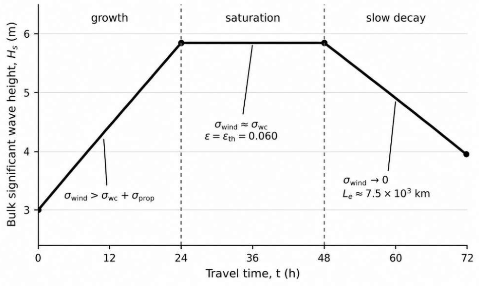
Figure 2.
Quantitative amplitude and steepness diagnostics for the representative long-range swell packet. (a) Evolution of bulk significant wave height over 72 h, showing growth, quasi-steady saturation near , and post-source decay toward approximately 4.0 m; (b) Corresponding bulk steepness , with the assumed threshold shown as a horizontal dashed line. The coincidence between the plateau and confirms the internal consistency of the reference envelope.
Figure 2.
Quantitative amplitude and steepness diagnostics for the representative long-range swell packet. (a) Evolution of bulk significant wave height over 72 h, showing growth, quasi-steady saturation near , and post-source decay toward approximately 4.0 m; (b) Corresponding bulk steepness , with the assumed threshold shown as a horizontal dashed line. The coincidence between the plateau and confirms the internal consistency of the reference envelope.
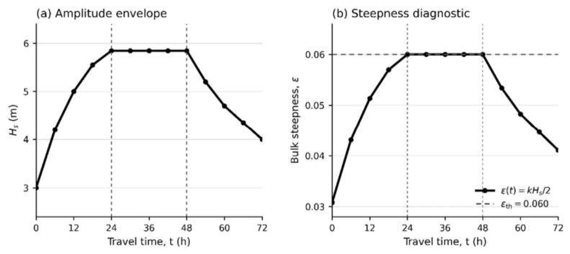
Figure 3.
Sensitivity of the steepness-limited saturation height to peak period and threshold steepness. The curves show for , 0.06 and 0.07. The marked reference case corresponds to and , giving . The quadratic dependence on shows why long-period swell can sustain larger significant wave heights before reaching the same steepness threshold.
Figure 3.
Sensitivity of the steepness-limited saturation height to peak period and threshold steepness. The curves show for , 0.06 and 0.07. The marked reference case corresponds to and , giving . The quadratic dependence on shows why long-period swell can sustain larger significant wave heights before reaching the same steepness threshold.
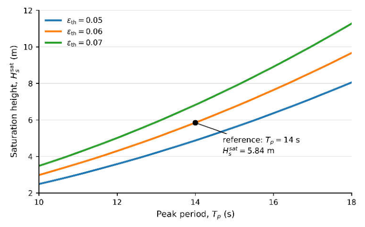
Figure 4.
Time evolution of quality-controlled Graciosa buoy observations over the analyzed period. Top panel: significant wave height . Middle panel: peak period . Bottom panel: bulk steepness , with indicated by a dashed line. Black markers identify energetic long-period records satisfying and .
Figure 4.
Time evolution of quality-controlled Graciosa buoy observations over the analyzed period. Top panel: significant wave height . Middle panel: peak period . Bottom panel: bulk steepness , with indicated by a dashed line. Black markers identify energetic long-period records satisfying and .
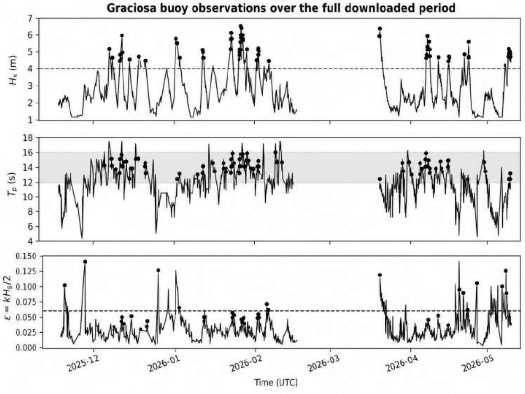
Figure 5.
Observed Graciosa buoy sea states relative to steepness-limited saturation curves. Grey points represent all quality-controlled buoy measurements, and black circles identify energetic long-period records satisfying and . The coloured curves show for , 0.06 and 0.07. The reference case , , and is indicated for comparison.
Figure 5.
Observed Graciosa buoy sea states relative to steepness-limited saturation curves. Grey points represent all quality-controlled buoy measurements, and black circles identify energetic long-period records satisfying and . The coloured curves show for , 0.06 and 0.07. The reference case , , and is indicated for comparison.
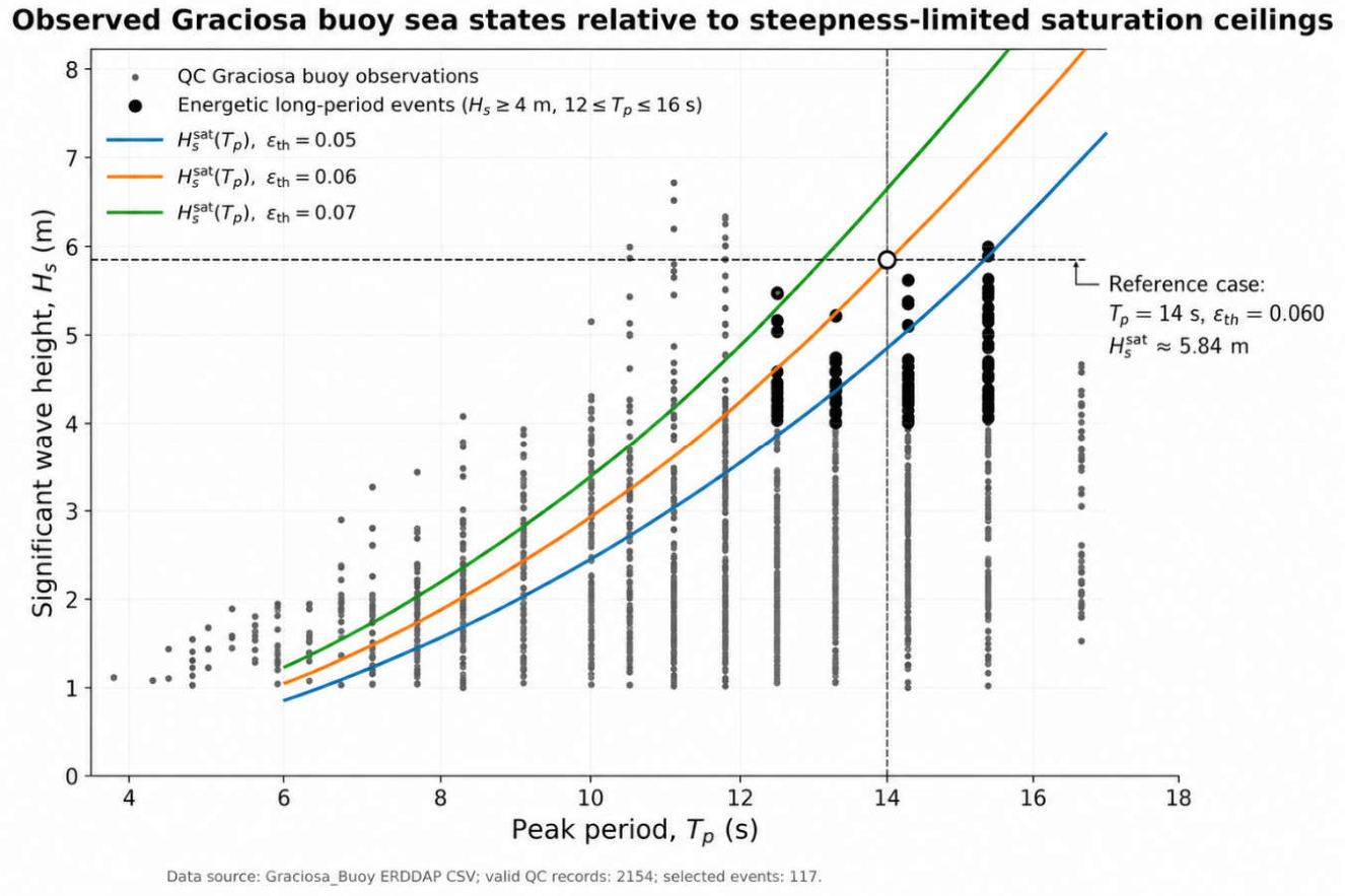

Table 1.
Sensitivity of the steepness-limited saturation height to peak period and threshold steepness .
Table 1.
Sensitivity of the steepness-limited saturation height to peak period and threshold steepness .
| TP (s) | for | for | for |
|---|---|---|---|
| 12 | 3.58 m | 4.29 m | 5.01 m |
| 14 | 4.87 m | 5.84 m | 6.82 m |
| 16 | 6.36 m | 7.63 m | 8.91 m |
Table 2.
Sensitivity of offshore arrival height to effective attenuation length , using and .
| Le (km) | |
|---|---|
| 3000 | 2.27 m |
| 5000 | 3.32 m |
| 7500 | 4.01 m |
| 10000 | 4.40 m |
| 20000 | 5.07 m |
Table 3.
Ten strongest energetic long-period events recorded at the Graciosa buoy.
| Peak time UTC |
(m) |
(s) | Direction (°) |
, (m) |
||
|---|---|---|---|---|---|---|
| 2026-01-26 23:08 | 5.98 | 15.4 | 352 | 0.0507 | 7.07 | 0.85 |
| 2026-01-23 12:08 | 5.62 | 15.4 | 82 | 0.0477 | 7.07 | 0.79 |
| 2026-01-27 19:08 | 5.52 | 15.4 | 138 | 0.0468 | 7.07 | 0.78 |
| 2026-04-06 22:17 | 5.48 | 15.4 | 39 | 0.0465 | 7.07 | 0.77 |
| 2026-03-19 21:17 | 5.46 | 12.5 | 345 | 0.0703 | 4.66 | 1.17 |
| 2026-01-27 15:08 | 5.37 | 14.3 | 97 | 0.0528 | 6.10 | 0.88 |
| 2026-04-23 02:17 | 5.15 | 12.5 | 110 | 0.0663 | 4.66 | 1.11 |
| 2026-01-02 10:08 | 5.03 | 12.5 | 45 | 0.0648 | 4.66 | 1.08 |
| 2026-02-02 12:08 | 4.73 | 13.3 | 48 | 0.0538 | 5.27 | 0.90 |
| 2026-01-29 08:08 | 4.68 | 15.4 | 352 | 0.0397 | 7.07 | 0.66 |
Disclaimer/Publisher’s Note: The statements, opinions and data contained in all publications are solely those of the individual author(s) and contributor(s) and not of MDPI and/or the editor(s). MDPI and/or the editor(s) disclaim responsibility for any injury to people or property resulting from any ideas, methods, instructions or products referred to in the content. |
© 2026 by the authors. Licensee MDPI, Basel, Switzerland. This article is an open access article distributed under the terms and conditions of the Creative Commons Attribution (CC BY) license (http://creativecommons.org/licenses/by/4.0/).
Copyright: This open access article is published under a Creative Commons CC BY 4.0 license, which permit the free download, distribution, and reuse, provided that the author and preprint are cited in any reuse.