

Submitted:
09 July 2026
Posted:
10 July 2026
You are already at the latest version
Abstract
Background. Routine laboratory tests provide multidimensional information about systemic physiology, but their interpretation is usually analyte-specific and may not capture cumulative abnormality burden across biological systems. A laboratory-derived Restorative Index (RI) framework has been formulated to transform normalized laboratory deviations into a bounded 0–100 score, where higher values indicate lower laboratory abnormality burden. This study applied the global and domain-specific RI framework to de-identified longitudinal clinical laboratory data and evaluated its computability, longitudinal behavior, domain decomposition, and exploratory predictability. Methods. This retrospective application study analyzed de-identified longitudinal laboratory and treatment/dose data. Eligible numeric laboratory values were transformed into normalized abnormality distances relative to reference intervals. Subject-date panels with at least five RI-eligible analytes were used to compute global RI. Domain-specific RIs were computed for predefined biological domains. Subject-date panels were classified as baseline, intermediate, follow-up, or single-record observations. Exploratory predictive models included regularized linear models, Bayesian regression, tree-based ensemble models, boosting models, support-vector regression, neural networks, and domain-to-global models. Cross-validation used subject-level grouping where repeated observations were present. Results. The RI framework was applied to 2,001 eligible subject-date panels. Baseline RI was available in 902 subjects, follow-up RI in 551 subjects, and intermediate RI in 306 subjects, contributing 548 intermediate RI rows. Median global RI increased from 59.66 at baseline to 61.72 at follow-up, with a median change of +2.52 and mean change of +3.28 RI points. Using a 5-point threshold, 227 subjects improved, 167 remained stable, and 157 declined. Global RI prediction was feasible but modest; the strongest global model predicted final RI from the latest known pre-follow-up RI using ExtraTrees, with cross-validated R2=0.417, MAE = 12.24, and RMSE = 15.23. Domain-specific prediction was stronger for renal/uric intermediate RI (R2=0.598) and hematology/CBC intermediate RI (R2=0.570). Same-date global RI could be partially estimated from domain-specific RI features, with the best model achieving R2=0.639, whereas future final global RI prediction from domain RI dynamics was weaker (R2=0.237). Conclusion. The RI framework was applicable to heterogeneous longitudinal laboratory data and provided a computable, trackable, and biologically decomposable summary of laboratory abnormality burden. Domain-specific RI improved interpretability and selected-domain predictability. These findings support RI as a retrospective laboratory-informatics framework, but RI changes should not be interpreted as treatment efficacy and require prospective external validation against clinical outcomes.
Keywords:
restorative index
; laboratory medicine
; clinical informatics
; longitudinal data
; abnormality burden
; machine learning
; predictive modeling
; reference intervals
; electronic health records
; domain-specific biomarkers
1. Background
Routine clinical laboratory testing is one of the most widely used sources of objective physiological information in medicine. Hematology, renal function, liver enzymes, electrolytes, metabolic markers, inflammatory markers, endocrine tests, coagulation indices, and urinalysis are commonly interpreted as discrete analytes, usually by comparing each result with its corresponding reference interval. Reference intervals are fundamental to laboratory medicine because they provide the context by which measured values are classified as expected or unexpected relative to a defined reference population [1,2]. However, this analyte-by-analyte approach can become difficult to interpret when a patient has many mild or moderate abnormalities distributed across multiple biological systems. A laboratory report may contain several values that are each only modestly abnormal, yet their cumulative burden may reflect a clinically meaningful state of systemic physiological dysregulation.
The interpretation of serial laboratory results is also more complex than a simple normal-versus-abnormal classification. In longitudinal care, clinicians frequently need to determine whether a patient is improving, deteriorating, or remaining stable over time. Concepts such as biological variation, index of individuality, and reference change values were developed because changes in laboratory values must be interpreted against the background of analytical imprecision and within-person physiological variation [3,4]. These concepts emphasize that the clinical meaning of a laboratory value depends not only on its position relative to a population reference interval, but also on its change relative to previous values from the same individual [3].
Several established clinical scoring systems demonstrate the value of converting multidimensional physiological information into interpretable summary scores. In critical care, APACHE II and SOFA use selected physiological, clinical, and biochemical variables to quantify illness severity or organ dysfunction [5,6]. APACHE II was developed as a severity-of-disease classification system based on acute physiological derangement, age, and chronic health status [5], while SOFA was designed to describe organ dysfunction across major organ systems in critically ill patients [6]. These systems show that composite physiological scores can support risk stratification, outcome prediction, and standardized comparison across patients or time points. However, these scores were developed primarily for acute illness and critical care contexts rather than for broad longitudinal quantification of laboratory abnormality burden in heterogeneous outpatient or mixed clinical populations.
A related conceptual precedent exists in the deficit-accumulation model of frailty and in allostatic load research. The frailty index summarizes health status as the proportion of accumulated deficits among a defined set of possible deficits [7]. Allostatic load, in parallel, attempts to quantify multisystem physiological dysregulation using biomarker patterns across neuroendocrine, cardiovascular, metabolic, inflammatory, and other domains [8]. These frameworks support the broader principle that the total burden of abnormalities across systems may be informative even when individual abnormalities are nonspecific. Nevertheless, existing deficit-accumulation and allostatic load approaches are not primarily designed to transform routine laboratory panels into a scalable, visit-level, laboratory-specific abnormality burden score.
Routine laboratory data are increasingly being used in statistical and machine-learning models for screening, prognosis, risk prediction, and clinical decision support. Reviews of machine learning in laboratory medicine emphasize that routinely collected laboratory values contain rich, structured information and can support predictive modeling when appropriate preprocessing, validation, interpretability, and clinical context are considered [9]. At the same time, prediction models based on clinical data are vulnerable to optimism bias, poor generalizability, leakage from repeated measurements, missingness-related artifacts, and insufficient external validation [10,11]. These concerns are particularly important when laboratory data are used longitudinally, because repeated observations from the same subject can inflate apparent model performance if validation is not performed at the subject level.
To address these gaps, we applied a laboratory-derived Restorative Index (RI) as a quantitative measure of laboratory abnormality burden. The RI framework first transforms each eligible laboratory value into a normalized abnormality distance relative to its reference interval. Values within the reference interval contribute no abnormality burden, whereas values below or above the interval contribute a positive deviation scaled by an analyte-specific normalization denominator. These deviations are then aggregated as a root-mean-square abnormality burden and transformed onto a bounded 0–100 index, where higher values indicate lower laboratory abnormality burden and an RI of 100 indicates that all included analytes are within their corresponding reference intervals.
A global RI provides a compact summary of systemic laboratory abnormality burden, but a single global score may obscure biologically distinct trajectories. For example, a patient may show improvement in renal markers while simultaneously showing worsening hematologic or inflammatory markers. In such a case, the global RI may appear stable even though the underlying biological domains are moving in different directions. We therefore extended the RI framework into domain-specific RIs, including hematology/CBC, renal/uric, liver/biliary, glycemic/insulin, lipid, inflammatory/immune, electrolyte/acid-base, thyroid, coagulation, vitamin D, prostate, and urinalysis domains. This domain-specific decomposition preserves the simplicity of a summary index while allowing organ-system-level interpretation of where abnormality burden arises.
The domain-specific formulation also enables a hierarchical view of laboratory physiology. At the lowest level, individual analytes are converted into normalized abnormality distances. These analyte-level distances can be aggregated within biological domains to form domain-specific RIs. Domain-specific RIs can then be used to interpret, approximate, or model the global RI. This creates a structured analytical pathway from raw laboratory values to organ-system subindices and finally to a global systemic abnormality burden score. Such a hierarchy may be preferable to a purely black-box predictive model because it retains biological interpretability and allows investigators to distinguish between systemic change and domain-specific change.
In addition to static RI computation, longitudinal RI modeling may provide insight into whether laboratory abnormality burden changes over time and whether future RI values can be predicted from baseline RI, previous RI, treatment timing, dose-related variables, and domain-specific RI profiles. Because clinical prediction models require careful validation and transparent reporting, the present work treats RI prediction as exploratory model-behavior analysis rather than as a definitive clinical decision tool [10,11]. The goal is not to claim therapeutic efficacy or to replace clinical interpretation, but to evaluate whether RI can serve as a mathematically coherent, biologically interpretable, and longitudinally modelable summary of laboratory abnormality burden.
In this study, we applied a previously formulated global and domain-specific RI framework [12] to de-identified longitudinal clinical laboratory data. Because the RI is based on reference-interval-normalized abnormality burden rather than disease-specific diagnostic criteria, the framework is intended to be disease-agnostic and potentially applicable across multiple clinical contexts in which routine laboratory panels are available. The specific objectives were: first, to assess computability of RI in heterogeneous longitudinal laboratory panels; second, to quantify baseline, intermediate, and follow-up RI trajectories; third, to decompose global RI into biological domains; fourth, to evaluate whether selected domain-specific RI trajectories are more predictable than global RI; fifth, to test whether domain-specific RIs reconstruct or predict global RI; and sixth, to examine exploratory predictive models using baseline, previous RI, time, treatment, and dose features. We hypothesized that domain-specific RI decomposition would improve biological interpretability and that selected domain-specific RI trajectories would be more predictable than the global RI because they represent more coherent physiological subsystems.
2. Methods
2.1. Study Design
This study was designed as a retrospective, de-identified application study of a previously formulated laboratory-derived Restorative Index framework. The primary aim was to apply the previously defined RI framework to longitudinal clinical laboratory data. The study was not designed as an interventional clinical trial and was not intended to evaluate treatment efficacy. Rather, the analysis focused on the application of the previously formulated RI framework, its longitudinal behavior, its decomposition into biological domains, and the feasibility of predicting intermediate and final RI values from baseline, previous RI, treatment-related, dose-related, and domain-specific features.
The RI equations and abnormality-distance framework were based on the previously described laboratory-derived RI methodology [12]. In the present study, these equations were applied without changing the core RI formulation. The current analysis therefore evaluates real-world application, longitudinal behavior, domain-specific decomposition, and exploratory predictability rather than proposing a new index formula.
The laboratory datasets used for the method-behavior evaluation were analyzed in de-identified form, as cleared by the Indonesian Molecular Innovation Foundation ethics committee (IMIF 01/SK/VI/2025). All participants had previously provided written informed consent permitting the use of their clinical and laboratory data for research purposes, with protection of personal privacy and confidentiality. Because this manuscript presents retrospective application and evaluation of a previously formulated laboratory-derived index, it does not report an interventional clinical trial or make therapeutic efficacy claims. The overall RI construction workflow, from raw laboratory values to normalized abnormality distances, global RI, domain-specific RI, and longitudinal predictive modeling, is summarized in Figure 1.
2.2. Data Sources and Dataset Structure
The analysis used two linked data sources: a longitudinal laboratory dataset and a treatment/dose dataset. The laboratory dataset contained subject identifiers, laboratory dates, analyte names, measured values, units, and reference interval information where available. The treatment/dose dataset contained subject-level or visit-level treatment information, including treatment timing, interval, treatment frequency, and dose-related variables. Subject identifiers were standardized before merging by harmonizing spacing, case, punctuation, and common name-format inconsistencies. Records that could not be reliably linked were retained for laboratory RI computation when possible but were excluded from treatment-response modeling if treatment or dose predictors were unavailable.
The unit of analysis for RI computation was the subject-date laboratory panel. A subject-date panel was defined as all eligible numeric laboratory measurements obtained from the same subject on the same laboratory date. When multiple rows for the same analyte were present on the same subject-date, the value judged most analytically usable was retained after numeric conversion and reference-interval parsing. This aggregation step was performed to ensure that RI values represented visit-level laboratory status rather than isolated laboratory rows.
The initial laboratory dataset contained 2,093 raw laboratory rows across 915 subjects. After laboratory cleaning, numeric conversion, reference interval parsing, analyte eligibility screening, and minimum-panel filtering, 2,001 eligible subject-date RI panels were retained for longitudinal analysis. Among these, 902 subjects had a baseline RI, 551 subjects had an eligible follow-up RI, and 306 subjects had at least one eligible intermediate RI. A total of 548 intermediate RI rows were available for intermediate RI modeling.
2.3. Laboratory Value Preprocessing
Laboratory values were first converted to numeric format. Non-numeric characters, reporting symbols, and unit annotations embedded in value fields were removed when the measured value could be unambiguously recovered. Values reported as qualitative, categorical, uninterpretable, or non-numeric were excluded from RI computation. Laboratory items without usable reference intervals or without a predefined normalization rule were also excluded from the primary RI calculation.
Reference intervals were parsed into lower and upper limits where possible. For analytes with two-sided reference intervals, both lower and upper limits were used. For analytes with one-sided reference limits, such as “less than” or “greater than” thresholds, the abnormality distance was computed only in the clinically abnormal direction. Values within the accepted reference interval were treated as normal and contributed zero abnormality burden. This approach follows the clinical logic of reference-interval interpretation, while transforming categorical normality into a continuous abnormality-distance scale [1,2].
2.4. Normalized Abnormality Distance
Following the previously formulated RI methodology [12], for each subject , date , and analyte , the measured laboratory value was denoted as . The lower and upper reference limits were denoted as and , respectively. A normalized abnormality distance, , was calculated as follows:
The normalized abnormality distance is therefore non-negative. A value of indicates that the analyte is within the reference interval. Increasing values of indicate increasing distance outside the reference interval. The direction of abnormality, whether below or above the interval, was recorded separately when needed for analyte-level interpretation, but the primary RI burden calculation used the absolute normalized abnormality distance.
2.5. Global Abnormality Burden
For each eligible subject-date panel, the global laboratory abnormality burden was calculated as the root-mean-square of all eligible normalized abnormality distances:
2.6. Global Restorative Index Formulation
The global Restorative Index was calculated according to the previously formulated inverse-burden transformation [12]:
A subject-date panel was retained for global RI computation only if it contained at least five RI-eligible numeric analytes:
This minimum-panel rule was applied to reduce instability from sparse panels and to ensure that the global RI reflected a multidimensional laboratory profile rather than one or two isolated analytes.
2.7. Baseline, Intermediate, and Follow-Up RI Definitions
For each subject, RI values were ordered chronologically. The earliest eligible RI was defined as the baseline RI:
The latest eligible RI was defined as the final follow-up RI:
Any eligible RI occurring between the baseline and final follow-up date was classified as an intermediate RI:
Subjects with only one eligible subject-date panel contributed to cross-sectional RI computation but not to baseline-to-follow-up change analysis. Subjects with at least two eligible RI panels contributed to baseline/follow-up analysis. Subjects with three or more eligible RI panels could additionally contribute to intermediate RI modeling and latest-known pre-follow-up prediction tasks.
The absolute RI change from baseline to follow-up was calculated as:
Subjects were descriptively categorized as improved, stable, or declined using a threshold of 5 RI points:
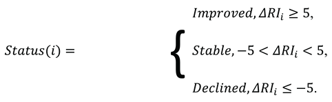
This categorical classification was used only for descriptive interpretation and was not used as the primary modeling target.
2.8. Domain-Specific RI Construction
To preserve biological interpretability, each eligible analyte was assigned to a predefined biological domain. The primary domains included hematology/CBC, renal/uric, liver/biliary, glycemic/insulin, lipid, inflammation/immune, electrolyte/acid-base, thyroid, coagulation, vitamin D, prostate, and urinalysis. Domain assignment was performed before modeling to avoid data-driven post hoc grouping.
For each domain , a domain-specific abnormality burden was computed as:
The domain-specific RI was then calculated as:
2.9. Domain-to-Global RI Reconstruction
Because the global RI and domain-specific RIs are both derived from the same analyte-level abnormality distances, a deterministic domain-to-global reconstruction was also evaluated. First, each domain RI was converted back to its corresponding burden:
The global burden was then approximated by recombining domain burdens using the number of analytes available in each domain as weights:
The reconstructed global RI was then calculated as:
This reconstruction analysis was interpreted separately from prognostic machine-learning models. It evaluates whether domain-specific RIs mathematically approximate the same-date global RI. It does not test whether domain-specific RIs predict future global RI.
2.10. Treatment, Timing, and Dose Predictors
Treatment and dose variables were included as exploratory covariates to evaluate modelability of RI trajectories. They were not used to infer treatment efficacy. In the treatment/dose dataset, GXM referred to a mixed gasotransmitter formulation composed of nitric oxide, carbon monoxide, and hydrogen sulfide in an intended ratio of . HHO referred to an oxyhydrogen formulation composed of hydrogen and oxygen in an intended ratio of . NO referred to nitric oxide exposure.
These variables were treated as retrospective exposure descriptors rather than causal treatment assignments. Dose-related features were summarized at the subject level, including average GXM dose, average HHO dose, average NO dose, treatment frequency, average treatment interval, days from baseline, and days to follow-up. Where appropriate, skewed dose variables were transformed using . Because the available dose fields may reflect recorded particle-based, volume-based, or derived average exposure measures rather than fully standardized per-session or cumulative biological dose, they were interpreted only as exploratory predictors in RI trajectory models. Time-dependent variables were calculated relative to the baseline laboratory date and the final follow-up laboratory date. For dynamic prediction tasks, the time interval between the latest known pre-follow-up RI and final follow-up RI was also included.
The phrase “latest known pre-follow-up RI” refers to the most recent eligible RI measurement before the final follow-up date. This value was used to represent the subject’s most recent observed laboratory trajectory before the final endpoint. It was not the final RI itself and therefore did not leak the target outcome into the model.
2.11. Predictive Modeling Tasks
Several predictive modeling tasks were defined. The first task was intermediate RI prediction, in which the target was an intermediate RI value and the predictors included baseline RI, previous RI, previous RI change, timing variables, treatment interval, treatment frequency, dose-related variables, and diagnosis/category where available:
The second task was final RI prediction from baseline information only:
The third task was dynamic final RI prediction from the latest known pre-follow-up RI:
The fifth task evaluated whether global RI could be estimated or predicted from domain-specific RI profiles. Same-date models estimated global RI from domain RIs measured on the same date, whereas prognostic models predicted final global RI from baseline domain RIs, latest pre-follow-up domain RIs, or domain RI dynamics:
and
2.12. Model Classes
Both interpretable and non-linear models were evaluated. Regularized and Bayesian linear models included Ridge regression, ElasticNetCV, and Bayesian Ridge regression. Non-linear ensemble models included Random Forest, ExtraTrees, Gradient Boosting, XGBoost, and LightGBM where available. Kernel-based and neural-network approaches included radial-basis-function support vector regression and multilayer perceptron regression. Naive comparator models were also evaluated, including baseline RI alone or previous RI alone, depending on the prediction task.
Linear models were included to provide interpretability and to assess whether RI trajectories were adequately described by additive predictor effects. Tree-based and boosting models were included to test non-linear predictor interactions. Neural-network models were evaluated as exploratory complex models but were not prioritized unless they improved cross-validated performance. Machine-learning implementation was performed using Python and scikit-learn, with additional compatible libraries where available [13].
2.13. Missing Data Handling
Missing laboratory values were not imputed for RI computation. RI was calculated only from analytes that were actually available and eligible in each subject-date panel. The number of analytes included in each RI calculation was retained as a coverage variable. This was important because different subject-date panels could contain different laboratory breadth, and RI interpretation may depend on the number and type of analytes available.
For predictive modeling, missing predictor values were handled within model pipelines using median imputation for continuous variables. Categorical variables, including diagnosis/category where available, were encoded using indicator variables. The imputation strategy was applied within the cross-validation pipeline to reduce information leakage. RI outcome values themselves were not imputed.
2.14. Cross-Validation and Leakage Prevention
Predictive performance was evaluated using cross-validation. For tasks with repeated observations per subject, folds were grouped at the subject level so that observations from the same subject did not appear in both training and validation folds. This was done to reduce within-subject leakage and overly optimistic performance estimates. The exploratory prediction analyses were reported with reference to PROBAST and TRIPOD+AI principles, recognizing that the present models were intended for model-behavior evaluation rather than clinical deployment [10,11].
For each modeling task, cross-validated predictions were generated and compared against observed RI values. The primary performance metric was the coefficient of determination:
Additional metrics included mean absolute error:
root mean squared error:
and mean bias:
Observed-versus-predicted plots, residual plots, and Bland–Altman plots were generated to visually assess model calibration, dispersion, systematic bias, and limits of agreement.
2.15. Model Interpretation and Feature Analysis
For regularized linear models, standardized coefficients were examined to identify the direction and relative magnitude of associations between predictors and RI outcomes. For tree-based models, feature importance values were extracted where available. These analyses were considered exploratory because model interpretability can be affected by collinearity, missingness, repeated measurements, and non-random treatment exposure.
Feature-importance results were therefore interpreted as model-behavior indicators rather than causal evidence. In particular, treatment and dose predictors were not interpreted as evidence of therapeutic efficacy. The observational design, lack of randomization, potential confounding by indication, and heterogeneous laboratory follow-up prevented causal inference.
2.16. Statistical Summaries
Continuous variables were summarized using mean, standard deviation, median, and interquartile range where appropriate. RI changes were summarized as absolute differences from baseline to follow-up and from baseline to intermediate visits. The number of subjects classified as improved, stable, or declined was reported descriptively using the predefined 5-point RI threshold. Domain-specific RI coverage was summarized by the number of eligible subject-date panels, number of subjects, number of analytes per domain, and the proportion of panels with sufficient domain data.
Model performance was summarized separately for global RI prediction, domain-specific RI prediction, and global RI prediction from domain-specific RI features. Same-date domain-to-global reconstruction was interpreted as a mathematical decomposition analysis, while final RI prediction from baseline or latest pre-follow-up predictors was interpreted as longitudinal prediction.
2.17. Software and Reproducibility
Data cleaning, RI computation, domain-specific RI construction, predictive modeling, cross-validation, and figure generation were performed in Python. The main computational libraries included pandas and NumPy for data processing, scikit-learn for machine-learning pipelines and cross-validation, and matplotlib for figure generation [13]. Output files included subject-date RI timelines, baseline/follow-up summaries, intermediate RI tables, domain-specific RI timelines, model-performance tables, cross-validated prediction files, feature-importance summaries, residual plots, Bland–Altman plots, and observed-versus-predicted figures.
3. Results
3.1. Applicability of the RI Framework to Longitudinal Laboratory Data
The Restorative Index (RI) framework was successfully applied to heterogeneous longitudinal laboratory data after preprocessing, numeric conversion, reference-interval parsing, and subject-date aggregation. Subject-date panels containing at least five RI-eligible numeric laboratory analytes were considered eligible for RI computation.
A total of 2,001 eligible subject-date panels were retained for analysis, representing repeated laboratory measurements across 902 subjects. Among these, 551 subjects had at least one eligible follow-up laboratory panel, while 306 subjects contributed one or more intermediate RI measurements, yielding 548 intermediate RI observations. Overall, 62 laboratory analytes spanning multiple biological systems were incorporated into the RI framework. Table 1 summarizes the composition of the analyzed dataset and the proportion of laboratory panels that could be converted into RI values.
These findings demonstrate that the RI framework is applicable to heterogeneous routine laboratory panels despite differences in analyte composition between subjects and visits. Rather than requiring identical laboratory panels, the RI could be computed from available eligible analytes, making it suitable for retrospective longitudinal datasets with variable laboratory coverage.
3.2. Longitudinal Behavior of the Global RI
After successful RI computation, longitudinal RI trajectories were examined by classifying each eligible subject-date panel as baseline, intermediate, or follow-up.
Among subjects with both baseline and follow-up RI values, the median global RI increased from 59.66 at baseline to 61.72 at follow-up. The median change was +2.52 RI points, while the mean change was +3.28 RI points. Using a descriptive threshold of five RI points, 227 subjects improved, 167 remained relatively stable, and 157 demonstrated declining RI values. Table 2A and Table 2B summarizes baseline, intermediate, and follow-up RI statistics.
The longitudinal behavior of the RI is illustrated in Figure 3, which shows both the cohort median trajectory and individual subject trajectories. Although the overall median RI increased modestly, individual trajectories were highly heterogeneous. Some subjects demonstrated sustained improvement, others remained relatively stable, and others exhibited progressive deterioration.
Intermediate RI measurements provided additional temporal resolution. A total of 548 intermediate RI observations were available from 306 subjects. Median intermediate RI was 54.97, while the mean intermediate RI was 58.38. Relative to baseline, intermediate RI increased by a median of +2.20 points and a mean of +3.19 points. Together, these observations indicate that the RI behaves as a longitudinal laboratory summary index capable of capturing both overall cohort trends and subject-specific variation.
3.3. Domain-Specific RI Decomposition
To improve biological interpretability, global RI was decomposed into predefined biological domains, including hematology/CBC, renal/uric, liver/biliary, glycemic/insulin, lipid, inflammatory/immune, electrolyte/acid-base, thyroid, coagulation, vitamin D, prostate, and urinalysis. Table 2 lists the analytes assigned to each biological domain.

Table 3.
Mapping of RI-eligible laboratory analytes to biological domains.
| Domain | Mapped analytes | RI-eligible analytes included in the domain |
|---|---|---|
| Hematology/CBC | 17 | Basophils, Eosinophils, Erythrocytes (Red Blood Cells), Granulocytes, Hematocrit, Hemoglobin, Leukocytes (White Blood Cells), Lymphocytes, Mean Corpuscular Hemoglobin (MCH), Mean Corpuscular Hemoglobin Concentration (MCHC), Mean Corpuscular Volume (MCV), Monocytes, Mean Platelet Volume (MPV), Neutrophils, Platelet Distribution Width (PDW), Red Cell Distribution Width (RDW), Platelets. |
| Renal/Uric | 5 | Uric acid, Blood urea nitrogen (BUN), Creatinine, Estimated glomerular filtration rate (eGFR), Urea |
| Liver/Biliary | 8 | Albumin, Total Bilirubin, Direct Bilirubin, Indirect Bilirubin, Alkaline Phosphatase (ALP), Gamma-Glutamyl Transferase (GGT), Aspartate Aminotransferase (AST), Alanine Aminotransferase (ALT) |
| Glycemic/Insulin | 6 | 2-hour Postprandial Plasma Glucose (2h-PPG), Random Plasma Glucose, Fasting Plasma Glucose, Hemoglobin A1c (HbA1c), Homeostatic Model Assessment of Insulin Resistance (HOMA-IR), Insulin |
| Lipid | 4 | HDL cholesterol, Total cholesterol, LDL cholesterol, Triglycerides |
| Inflammation/Immune | 3 | C-reactive protein (CRP), High-sensitivity C-reactive protein (hs-CRP), Erythrocyte sedimentation rate (ESR) |
| Electrolyte/Acid-base | 7 | Ionized Calcium, Ionized Magnesium, Potassium, Chloride, Total Magnesium, Sodium, pH |
| Thyroid | 5 | Free triiodothyronine (Free T3), Free thyroxine (Free T4), Triiodothyronine (T3), Thyroxine (T4), Thyroid-stimulating hormone (TSH) |
| Coagulation | 2 | International Normalized Ratio (INR), Prothrombin Time (PT) |
| Vitamin D | 1 | 25-Hydroxyvitamin D [25(OH)D] |
| Prostate | 1 | Prostate-specific antigen (PSA) |
| Urinalysis | 1 | Urine pH |
Domain coverage differed considerably across the dataset because laboratory testing was performed according to clinical need rather than a standardized protocol. Hematology/CBC and renal/uric domains contained the largest number of longitudinal observations, whereas thyroid, vitamin D, prostate, coagulation, and urinalysis domains were available less consistently. Despite these differences, domain-specific RI computation was feasible across all predefined domains whenever sufficient analytes were available. This decomposition enabled biological interpretation beyond the global RI by identifying the organ systems contributing most strongly to overall laboratory abnormality burden. For example, a patient with an unchanged global RI could simultaneously demonstrate improving renal RI, worsening hematology RI, and stable liver RI. Such patterns would be obscured if only the global RI were considered.
3.4. Exploratory Predictive Modeling of RI Trajectories
Because RI represents a longitudinal summary of laboratory abnormality burden, exploratory analyses were performed to determine whether future RI values could be predicted from baseline RI, previous RI, treatment-related variables, timing variables, dose-related variables, and domain-specific RI profiles. Prediction was considered a secondary exploratory endpoint rather than the primary objective of this study.
Among global RI models, intermediate RI prediction achieved cross-validated values of approximately 0.25. Final RI prediction from baseline information achieved , whereas prediction using the latest known pre-follow-up RI achieved the strongest overall performance (). Table 4 summarizes predictive performance across all global RI tasks, while Figure 4 illustrates observed-versus-predicted RI values for the principal prediction models.
Overall, prediction performance was modest, indicating that global laboratory abnormality burden contains measurable temporal structure but remains influenced by substantial biological and clinical variability that was not captured by the available predictors.
3.5. Domain-Specific RI Trajectories
Exploratory prediction was also performed separately for individual biological domains. Prediction accuracy differed substantially between domains. Renal/uric and hematology/CBC RI trajectories consistently demonstrated the strongest predictive performance across multiple modeling tasks. Intermediate renal/uric RI prediction achieved a cross-validated of 0.598, while hematology/CBC intermediate RI prediction achieved . Final RI prediction using the latest known pre-follow-up value also exceeded global RI performance for both domains.
These results are summarized in Table 5, while Figure 5 provides a heatmap of prediction performance across all evaluated biological domains.
The stronger performance of selected domains suggests that organ-system-specific laboratory abnormalities follow more coherent longitudinal trajectories than the aggregate systemic RI.
3.6. Hierarchical Relationship Between Domain-Specific and Global RI
Finally, the hierarchical structure of the RI framework was evaluated by determining whether domain-specific RI profiles could explain or predict the global RI. Same-date global RI reconstruction from domain-specific RI values performed well, with the best model achieving a cross-validated of 0.639. In contrast, prediction of future global RI from baseline domain-specific RI values or domain-specific RI dynamics showed substantially weaker performance, with values ranging from approximately 0.21 to 0.24. These results are summarized in Table 6 and illustrated in Figure 6.
The findings suggest that domain-specific RIs primarily function as explanatory components of the global RI rather than independent longitudinal predictors. In other words, domain-specific RI values effectively describe the current composition of laboratory abnormality burden but only partially explain its future evolution.
4. Discussion
4.1. Principal Findings
This study applied a previously formulated laboratory-derived Restorative Index (RI) framework to de-identified longitudinal clinical laboratory data. The RI framework converted heterogeneous routine laboratory panels into a scalar global abnormality burden score on a clinically intuitive 0–100 scale, where higher values indicate lower laboratory abnormality burden. This allowed laboratory analytes with different units, reference ranges, and physiological meanings to be integrated into a single visit-level index.
The RI framework was applicable to real-world longitudinal laboratory data and enabled baseline, intermediate, and follow-up trajectories to be quantified. Among subjects with both baseline and follow-up RI values, median global RI increased modestly from 59.66 at baseline to 61.72 at follow-up, with a median change of +2.52 points and a mean change of +3.28 points. However, individual trajectories were heterogeneous: 227 subjects improved by at least 5 RI points, 167 were stable, and 157 declined by at least 5 RI points. These findings suggest that RI can capture both cohort-level trends and subject-level variability in laboratory abnormality burden over time.
Exploratory predictive modeling of global RI was feasible but modest. Final RI prediction from baseline features achieved , while dynamic final RI prediction using the latest known RI trajectory achieved . The strongest global RI model incorporated the latest known pre-follow-up RI, with ExtraTrees reaching . This suggests that recently observed laboratory trajectory carries important predictive information beyond baseline status and treatment exposure alone. Nevertheless, substantial unexplained variance remained, consistent with biological heterogeneity, variable laboratory follow-up, non-standardized testing patterns, and unmeasured clinical factors.
Domain-specific RI modeling provided an important extension of the global RI. Renal/uric and hematology/CBC domains showed stronger predictive performance than the global aggregate, with intermediate RI prediction reaching and , respectively. Same-date domain-specific RIs also partially reconstructed the global RI, with same-date domain-to-global prediction reaching using domain RI values alone and improving slightly when domain coverage counts were included. These findings support a hierarchical interpretation of the RI framework: analyte-level abnormality distances can be aggregated into domain-specific RIs, and domain-specific RIs can explain a substantial portion of the global RI.
Taken together, the results support RI as an applicable, disease-agnostic framework for retrospective laboratory trajectory analysis. The global RI provides a compact summary of systemic laboratory abnormality burden, while domain-specific RIs provide biological interpretability across organ-system domains. Because the framework depends on normalized deviation from reference intervals rather than on disease-specific endpoints, it may be adaptable to diverse clinical contexts, including chronic disease monitoring, multimorbidity assessment, aging-related research, rehabilitation cohorts, and retrospective laboratory analytics. However, future global RI prediction remained limited, indicating that RI trajectories are influenced by unmeasured biological, clinical, measurement, and treatment-response heterogeneity.
4.2. Biological Interpretability of Domain-Specific RI
The global RI summarizes systemic laboratory abnormality burden, but domain-specific RI explains where that burden comes from. This distinction is important because a single global score can obscure biologically meaningful differences between organ systems. A patient may show improved renal RI, worsened hematology/CBC RI, and stable liver RI, resulting in little net change in the global RI. In such a case, a global-only interpretation may classify the trajectory as stable, whereas domain-specific decomposition reveals a biologically important redistribution of abnormality burden.
The stronger predictive performance observed in renal/uric and hematology/CBC domains may reflect both methodological and biological factors. These domains are commonly measured in routine practice, resulting in more complete longitudinal coverage and more stable domain RI estimates. They also contain physiologically related analytes. The renal/uric domain includes creatinine, urea, BUN, estimated glomerular filtration rate, and uric acid, which are linked through renal filtration and nitrogen metabolism. The hematology/CBC domain includes hemoglobin, hematocrit, red blood cell indices, white blood cell counts, platelets, and differential counts, which collectively reflect hematopoietic, inflammatory, and circulating-cell status.
Domain-specific RI may therefore improve signal coherence by reducing biological heterogeneity. The global RI aggregates abnormalities across renal, hepatic, hematologic, metabolic, inflammatory, endocrine, coagulation, electrolyte, and urinalysis domains, which may change independently or in opposite directions. By contrast, domain-specific RIs isolate narrower physiological subsystems and may therefore have stronger signal-to-noise ratios. The higher predictability of renal/uric and hematology/CBC RIs should not be interpreted as evidence that these domains are universally more important than others; rather, it indicates that, in this dataset, these domains had more complete measurement density and more coherent longitudinal structure.
4.3. Interpretation of Predictive Modeling
Non-linear and complex models were evaluated to determine whether RI trajectories contained interactions or non-additive relationships not captured by regularized linear models. These included ensemble tree models, boosting models, kernel-based regression, and neural-network models. However, complex models did not uniformly outperform simpler models. In several global RI prediction tasks, ElasticNetCV or other regularized linear approaches performed as well as or better than more complex methods.
This limited superiority of complex models suggests that much of the predictable RI variance was captured by baseline RI, previous RI, RI change, time interval, and treatment timing. More flexible models may offer only incremental benefit when these trajectory features are already included, especially in heterogeneous retrospective datasets with variable follow-up, sparse predictors, and non-random missingness. The clearest non-linear advantage was observed when the latest known pre-follow-up RI was included, suggesting that complex models may be useful when richer trajectory information is available.
These findings support the use of interpretable models as the primary analytic reference and non-linear models as exploratory sensitivity analyses. The RI itself is mathematically transparent, and its clinical value depends partly on interpretability. Highly flexible models may require larger, more standardized prospective datasets before they can be considered reliable. The use of subject-level cross-validation was important because prediction models in longitudinal clinical data are vulnerable to overfitting, data leakage, optimism bias, and poor generalizability if validation is not carefully designed [10,11].
4.4. Clinical and Research Implications
The RI framework may be useful as a disease-agnostic tool for retrospective laboratory trajectory monitoring, systemic abnormality burden quantification, patient-level longitudinal visualization, and domain-specific interpretation of laboratory change. Rather than replacing analyte-level interpretation or disease-specific endpoints, RI provides a complementary summary of overall laboratory abnormality burden and its organ-system components. In research settings, RI may serve as an exploratory endpoint, a stratification variable, or a framework for comparing laboratory trajectories across heterogeneous clinical populations. This broader applicability may be particularly relevant for studies involving multimorbidity, aging, chronic disease, rehabilitation, or longitudinal clinical phenotyping, where laboratory abnormalities often span multiple biological systems rather than a single disease category.
4.5. Not A Clinical Efficacy Claim
A critical limitation of interpretation is that the present study does not establish treatment efficacy. The dataset was retrospective, non-randomized, and application-focused. Treatment exposure, dose, frequency, and timing were not assigned randomly, and subjects may have differed in baseline condition, indication, disease severity, follow-up frequency, laboratory ordering patterns, concurrent care, and unmeasured clinical events. These factors can confound any apparent association between treatment variables and RI change. Therefore, RI changes should not be interpreted as evidence that any specific treatment caused improvement or decline. A subject’s RI may change because of natural disease course, regression to the mean, concurrent medical care, differences in laboratory testing, hydration or nutritional status, acute illness, medication changes, or other unmeasured factors. The present analysis demonstrates that RI can be computed, tracked, decomposed into biological domains, and modeled longitudinally. It does not prove that treatment exposure caused RI improvement.
The appropriate interpretation is methodological and applicative: the RI framework provides a feasible way to quantify laboratory abnormality burden from heterogeneous routine laboratory data, and RI trajectories show measurable longitudinal behavior. Predictive models demonstrate that some aspects of RI variation are modelable, especially when prior trajectory information or domain-specific structure is included. However, causal claims require prospective study designs with standardized laboratory panels, predefined endpoints, controlled treatment exposure, and appropriate comparison groups.
Because the present analysis is retrospective, non-randomized, and application-focused, RI changes should not be interpreted as treatment efficacy. Rather, they demonstrate the applicability of RI computation, the interpretability of domain-specific decomposition, and the exploratory modelability of RI trajectories.
4.6. Future Validation and Implementation
Future work should focus on validating the RI framework under more standardized and clinically interpretable conditions. First, prospective studies should apply the RI framework using a predefined laboratory panel measured at standardized time points. This would reduce variability caused by heterogeneous laboratory ordering and allow global and domain-specific RI trajectories to be compared more directly across subjects and visits.
Second, external validation is needed in independent datasets. The present analysis used a single retrospective dataset, and internal cross-validation cannot establish generalizability. Future studies should test whether RI computation, domain-specific decomposition, and predictive model performance remain stable across different laboratories, populations, reference intervals, assay platforms, and clinical settings.
Third, RI should be validated against clinically meaningful outcomes. Future studies should examine whether baseline RI, longitudinal RI change, or domain-specific RI trajectories correlate with symptoms, functional status, hospitalization, disease-specific outcomes, imaging biomarkers, frailty measures, or biological aging markers. Such analyses are necessary to determine whether RI is only a laboratory abnormality burden score or whether it also reflects clinically relevant physiological status.
Fourth, a minimal standardized RI panel should be developed. Although the full RI framework can incorporate many analytes, practical implementation would benefit from identifying a smaller set of laboratory tests that preserves most of the information contained in the broader index. This minimal panel should be statistically informative, clinically balanced across major physiological domains, and feasible for routine prospective use.
Fifth, refined longitudinal modeling approaches should be explored. Mixed-effects models, Bayesian hierarchical models, time-series models, uncertainty intervals, domain-weighted RI formulations, and clinically constrained machine-learning models may improve interpretability and predictive performance. These refinements should be developed in larger prospective datasets and evaluated using transparent validation procedures.
Together, these future directions will determine whether RI can progress from a retrospective laboratory trajectory framework to a validated longitudinal biomarker. Until such validation is completed, RI should be regarded as an applicable research tool for summarizing and modeling laboratory abnormality burden rather than as a standalone clinical decision instrument.
5. Limitations
This study has several important limitations that should be considered when interpreting the RI framework, the longitudinal RI trajectories, and the predictive modeling results. First, the analysis was based on a retrospective dataset. Laboratory tests, follow-up intervals, treatment exposure, and dose schedules were not prospectively standardized. As a result, the available data reflect real-world clinical and operational patterns rather than a controlled study protocol. Retrospective data are useful for application and longitudinal model-behavior evaluation study, but they are inherently limited for causal inference and prospective clinical decision-making.
Second, treatment exposure was non-randomized. Subjects were not assigned to treatment groups under a randomized or controlled design, and treatment frequency, interval, and dose may have been influenced by clinical condition, patient preference, physician decision-making, availability, disease severity, or follow-up behavior. Therefore, associations between treatment-related variables and RI change should not be interpreted as evidence of treatment efficacy. Any apparent relationship between treatment exposure and RI trajectory may be confounded by indication, baseline health status, concurrent care, or unmeasured clinical factors.
Third, selection bias may be present. Subjects who had repeated laboratory measurements and sufficient laboratory coverage to compute RI may differ systematically from subjects with sparse or incomplete laboratory data. For example, patients undergoing closer clinical monitoring may have more severe illness, greater clinical concern, better adherence, or greater access to follow-up testing. These factors could influence both RI computation and longitudinal RI behavior. Therefore, the analyzed cohort may not represent the broader population from which the data were drawn.
Fourth, laboratory panels were not uniform across subjects or visits. The RI framework was designed to accommodate heterogeneous laboratory panels, but this flexibility also introduces interpretive complexity. A global RI calculated from a broad panel containing hematology, renal, liver, metabolic, inflammatory, and electrolyte markers is not identical in information content to a global RI calculated from a narrower panel. Although a minimum requirement of five eligible analytes was used to reduce instability from sparse panels, the number and type of analytes contributing to RI still varied across subject-date panels.
Fifth, missingness may be clinically informative. In routine clinical data, laboratory values are not missing at random. A test may be absent because it was clinically unnecessary, unavailable, too costly, not ordered, or not repeated after normalization. Conversely, abnormal or clinically concerning domains may be tested more frequently. Therefore, missing analytes may carry information about clinical status, physician concern, or care patterns. The present analysis did not fully model informative missingness. Instead, RI was calculated from available eligible analytes, and analyte/domain coverage was retained descriptively.
Sixth, domain-specific RI coverage varied by subject, visit, and biological domain. Domains such as hematology/CBC and renal/uric markers were more frequently available and therefore more suitable for longitudinal modeling. Other domains, including thyroid, vitamin D, prostate markers, coagulation, and some inflammatory markers, had more limited or irregular coverage. Differences in domain coverage may partly explain why renal/uric and hematology/CBC models performed better than other domain models. Therefore, stronger performance in these domains should not be interpreted solely as biological superiority; it may also reflect better measurement density and more complete longitudinal data.
Seventh, treatment and dose variables may be incomplete, heterogeneous, or confounded. Treatment count, interval, frequency, and dose-related variables were extracted from available treatment/dose records, but these variables may not fully capture actual biological exposure. They may not reflect adherence, administration quality, timing relative to laboratory testing, concurrent therapies, acute illness, diet, hydration, medication changes, or other clinical events. Dose variables may also be correlated with baseline severity or treatment indication. Consequently, treatment/dose predictors should be interpreted as exploratory covariates rather than causal exposure variables.
Eighth, no external validation cohort was available. All RI computation, domain-specific RI construction, trajectory analysis, and predictive modeling were performed within the available dataset. Although cross-validation was used, internal validation cannot replace external validation. Model performance may decline when applied to independent populations, different laboratories, different reference intervals, different clinical settings, or prospectively collected datasets. External validation will be necessary before the RI framework or predictive models can be considered generalizable.
Ninth, reference intervals may vary by laboratory, assay method, population, sex, age, and clinical context. The RI framework depends on reference intervals to define abnormality distances. If reference intervals differ across laboratories or are not adjusted for relevant biological factors, RI values may vary even for the same measured analyte values. Some analytes have age- or sex-specific reference ranges, while others depend on assay platform or laboratory calibration. Future implementations should incorporate standardized reference-interval handling, including age-, sex-, method-, and laboratory-specific reference ranges where appropriate.
Tenth, the RI has not yet been validated against hard clinical outcomes. The present analysis evaluated whether RI could be computed, tracked longitudinally, decomposed into biological domains, and modeled statistically. It did not test whether RI predicts mortality, hospitalization, disease progression, functional status, frailty, imaging outcomes, quality of life, or other clinically meaningful endpoints. Without outcome validation, RI should be interpreted as a laboratory abnormality burden index rather than a validated clinical outcome measure.
Eleventh, the predictive models are exploratory and not clinical-grade. Although multiple model classes were evaluated, including regularized linear models, ensemble models, boosting methods, kernel models, and neural networks, the models were developed for method-behavior analysis rather than clinical deployment. The observed cross-validated performance was modest for global RI prediction and stronger only in selected domain-specific tasks. The models may be sensitive to missingness, panel composition, small subgroup sizes, predictor collinearity, and retrospective sampling. They should therefore not be used to guide clinical decisions without prospective validation, calibration assessment, external testing, and evaluation of clinical utility.
Finally, the present RI formulation uses a specific mathematical structure: normalized abnormality distances, root-mean-square aggregation, and inverse transformation onto a 0–100 scale. This formulation is transparent and clinically interpretable, but it is not the only possible formulation. Alternative weighting schemes, analyte-specific clinical importance weights, direction-sensitive penalties, age-adjusted normalization, Bayesian uncertainty intervals, or disease-specific domain weights may improve performance in future studies. The current formulation should therefore be regarded as a first-generation RI framework requiring further refinement and validation.
In summary, the limitations of this study are primarily related to its retrospective design, heterogeneous laboratory coverage, non-randomized treatment exposure, lack of external validation, and absence of hard clinical outcome validation. These limitations do not invalidate the methodological contribution of the RI framework, but they do constrain interpretation. The present findings support RI as a feasible and modelable laboratory abnormality burden index, while future prospective studies are required to establish generalizability, clinical validity, and practical utility.
6. Conclusion
This study applied a previously formulated laboratory-derived Restorative Index framework to de-identified longitudinal clinical laboratory data. The global RI provided a compact summary of systemic laboratory abnormality burden, while domain-specific RIs revealed biologically interpretable organ-system trajectories. The framework was computable across heterogeneous subject-date panels and showed modest but measurable longitudinal predictability, particularly when recent RI trajectory information was included. Selected domain-specific RIs, especially renal/uric and hematology/CBC indices, showed stronger predictability than the global aggregate. These findings support RI as an applicable disease-agnostic framework for retrospective laboratory trajectory analysis across multiple clinical contexts, while prospective external validation and clinical outcome correlation remain necessary before clinical deployment.
Funding
No external funding was received for this study.
Ethics approval and consent to participate
The laboratory datasets used in this retrospective application study were analyzed in de-identified form, as approved by the Indonesian Molecular Innovation Foundation Ethics Committee (IMIF 01/SK/VI/2025). The study was conducted in accordance with the ethical principles of the Declaration of Helsinki and applicable Indonesian regulations governing research involving human participants. All participants had previously provided written informed consent permitting the use of their clinical and laboratory data for research purposes, with protection of personal privacy and confidentiality. Because this manuscript presents a retrospective application and evaluation of a previously formulated laboratory-derived index, it does not report an interventional clinical trial or evaluate treatment efficacy.
Consent for publication
Not applicable. The manuscript does not contain identifiable individual person data, images, or videos.
Availability of data and materials
The raw de-identified clinical laboratory dataset is not publicly available because of privacy and ethics restrictions. To support reproducibility, the RI computation equations, analyte-to-domain mapping, aggregate RI outputs, model-performance tables, and analytic scripts can be provided by the corresponding author on reasonable request, subject to institutional approval.
Competing interests
The author declares that he has no competing interests.
Authors’ contributions
ATH conceptualized the study, developed the application framework, curated and analyzed the data, interpreted the results, prepared the figures and tables, drafted the manuscript, revised the manuscript critically for intellectual content, and approved the final version for submission.
Acknowledgments
The author acknowledges the Indonesian Molecular Innovation Foundation for administrative and ethics support. The author also acknowledges the participants whose de-identified laboratory data contributed to this retrospective analysis. The author used ChatGPT, an AI language model developed by OpenAI, for editorial assistance, language refinement, manuscript organization, and drafting support. The author reviewed, verified, and takes full responsibility for all manuscript content, analyses, interpretations, references, and conclusions.
Authors’ information
Aditya Tri Hernowo is affiliated with the Indonesia Molecular Innovation Foundation, Malang, Indonesia, and Universitas Islam Indonesia, Yogyakarta, Indonesia.
List of Abbreviations
ALP: Alkaline phosphatase
ALT: Alanine aminotransferase
AST: Aspartate aminotransferase
BUN: Blood urea nitrogen
CBC: Complete blood count
CO: Carbon monoxide
CRP: C-reactive protein
eGFR: Estimated glomerular filtration rate
ESR: Erythrocyte sedimentation rate
GGT: Gamma-glutamyl transferase
GXM: Gasotransmitter mixture
HbA1c: Hemoglobin A1c
HHO: Oxyhydrogen formulation
HOMA-IR: Homeostatic Model Assessment of Insulin Resistance
hs-CRP: High-sensitivity C-reactive protein
INR: International normalized ratio
MAE: Mean absolute error
ML: Machine learning
MPV: Mean platelet volume
NO: Nitric oxide
PDW: Platelet distribution width
PT: Prothrombin time
RDW: Red cell distribution width
RI: Restorative Index
RMSE: Root mean squared error
TRIPOD: Transparent Reporting of a multivariable prediction model for Individual Prognosis Or Diagnosis
TSH: Thyroid-stimulating hormone
References
- Ozarda, Y. Reference intervals: current status, recent developments and future considerations. Biochem Med 2016. [Google Scholar] [CrossRef]
- Ceriotti, F. Prerequisites for use of common reference intervals. Clin. Biochem Rev. 2007. [Google Scholar] [PubMed]
- Sithiravel, C.; et al. Biological variation, reference change values and index of individuality. Biochem Med 2021. [Google Scholar] [CrossRef]
- Sandberg, S.; et al. Biological variation: recent developments and future challenges. Clin Chem Lab Med 2022. [Google Scholar] [CrossRef] [PubMed]
- Knaus, W.A.; Draper, E.A.; Wagner, D.P.; Zimmerman, J.E. APACHE II: a severity of disease classification system. Crit Care Med 1985. [Google Scholar] [CrossRef] [PubMed]
- Vincent, J.L.; et al. The SOFA score to describe organ dysfunction/failure. Intensive Care Med 1996. [Google Scholar] [CrossRef] [PubMed]
- Rockwood, K.; Mitnitski, A. Frailty in relation to the accumulation of deficits. J. Gerontol. A Biol. Sci. Med. Sci. 2007. [Google Scholar] [CrossRef] [PubMed]
- Beese, S.; et al. Allostatic load measurement: a systematic review of reviews. Psychosom Med 2022. [Google Scholar] [CrossRef]
- Rabbani, N.; et al. Applications of machine learning in routine laboratory medicine. Clin. Biochem 2022. [Google Scholar] [CrossRef] [PubMed]
- Moons, K.G.M.; et al. PROBAST: a tool to assess risk of bias and applicability of prediction model studies. Ann Intern Med. [CrossRef] [PubMed]
- Collins, G.S.; Moons, K.G.M.; Dhiman, P.; Riley, R.D.; Beam, A.L.; Van Calster, B.; Ghassemi, M.; Liu, X.; Reitsma, J.B.; van Smeden, M.; Boulesteix, A.L.; et al. TRIPOD+AI statement: updated guidance for reporting clinical prediction models that use regression or machine learning methods. BMJ 2024, 385, e078378. [Google Scholar] [CrossRef] [PubMed]
- Hernowo, A.T. Generalizable laboratory-derived restorative index for cross-clinical assessment of systemic laboratory abnormality burden. Unpublished manuscript. 2026.
- Pedregosa, F.; Varoquaux, G.; Gramfort, A.; Michel, V.; Thirion, B.; Grisel, O.; et al. Scikit-learn: machine learning in Python. J. Mach. Learn Res. 2011, 12, 2825–2830. [Google Scholar]
Figure 1.
Conceptual diagram of Restorative Index construction. Raw laboratory values are first converted into eligible numeric analytes and interpreted relative to their reference intervals. Each analyte is transformed into a normalized abnormality distance, where values within the reference interval contribute zero abnormality burden and values outside the interval contribute a positive scaled deviation. These analyte-level abnormality distances are aggregated into a global abnormality burden and transformed into the global Restorative Index (RI). The same abnormality-distance framework is also applied within biological domains to generate domain-specific RIs. Global and domain-specific RIs are then used for baseline, intermediate, and follow-up trajectory analysis, as well as predictive modeling of intermediate and final RI values.
Figure 1.
Conceptual diagram of Restorative Index construction. Raw laboratory values are first converted into eligible numeric analytes and interpreted relative to their reference intervals. Each analyte is transformed into a normalized abnormality distance, where values within the reference interval contribute zero abnormality burden and values outside the interval contribute a positive scaled deviation. These analyte-level abnormality distances are aggregated into a global abnormality burden and transformed into the global Restorative Index (RI). The same abnormality-distance framework is also applied within biological domains to generate domain-specific RIs. Global and domain-specific RIs are then used for baseline, intermediate, and follow-up trajectory analysis, as well as predictive modeling of intermediate and final RI values.
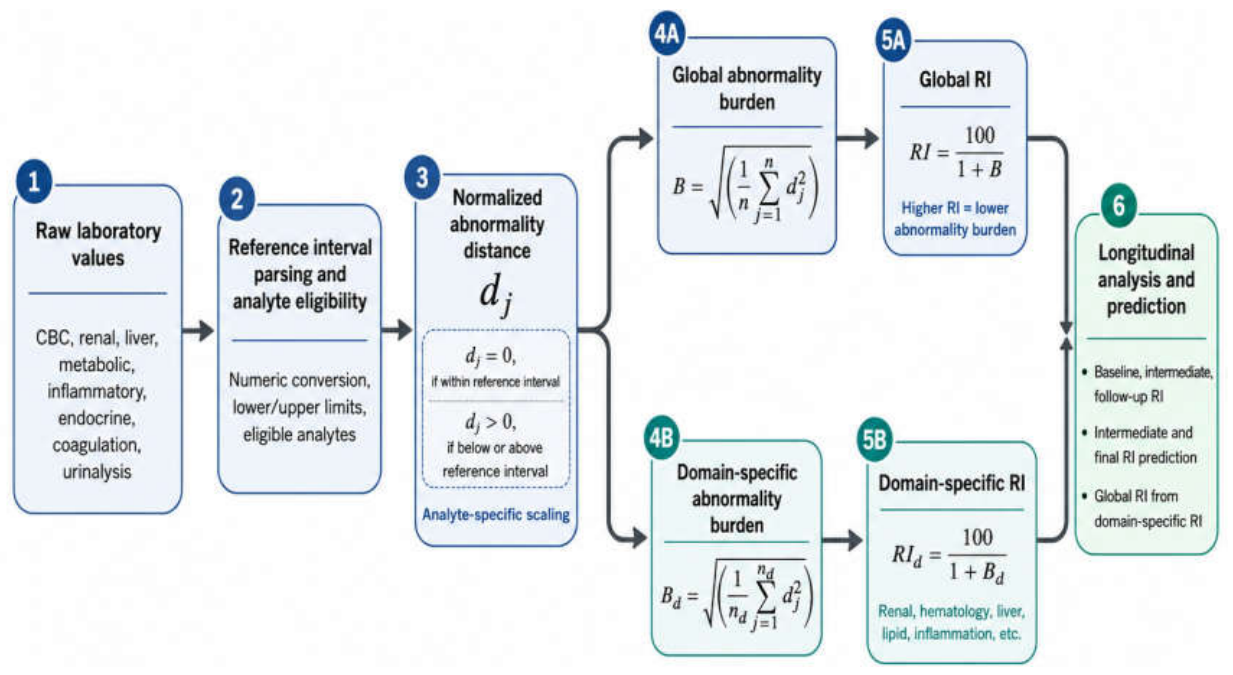
Figure 2.
Restorative Index formula and interpretation scale. The global abnormality burden B is calculated as the root-mean-square of normalized analyte-level abnormality distances dj. Analytes within their reference intervals contribute dj=0, whereas analytes below or above their reference intervals contribute positive scaled deviations. The Restorative Index is then calculated as RI = 100/(1+B), producing a bounded 0–100 score in which higher values indicate lower laboratory abnormality burden. When B = 0, all included analytes are within their reference intervals and RI = 100. As B increases, RI decreases nonlinearly; for example, B = 0.5 corresponds to RI = 66.7, B = 1 corresponds to RI = 50, and B = 4 corresponds to RI = 20.
Figure 2.
Restorative Index formula and interpretation scale. The global abnormality burden B is calculated as the root-mean-square of normalized analyte-level abnormality distances dj. Analytes within their reference intervals contribute dj=0, whereas analytes below or above their reference intervals contribute positive scaled deviations. The Restorative Index is then calculated as RI = 100/(1+B), producing a bounded 0–100 score in which higher values indicate lower laboratory abnormality burden. When B = 0, all included analytes are within their reference intervals and RI = 100. As B increases, RI decreases nonlinearly; for example, B = 0.5 corresponds to RI = 66.7, B = 1 corresponds to RI = 50, and B = 4 corresponds to RI = 20.
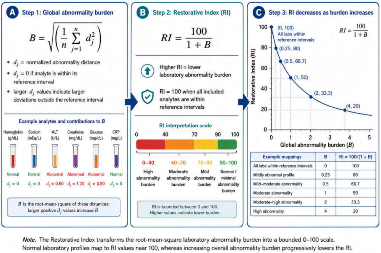
Figure 3.
Baseline, intermediate, and follow-up global Restorative Index trajectories. Panel A shows individual subject-level global RI trajectories across baseline, intermediate, and follow-up stages, with faint gray spaghetti lines representing individual longitudinal patterns and the dark-blue line representing the cohort median trajectory. Median RI values were 59.66 at baseline, 54.97 at intermediate visits, and 61.72 at follow-up. Panel B shows stage-wise global RI distributions using violin and boxplot summaries, with the median trajectory overlaid. The figure demonstrates a modest overall median increase from baseline to follow-up, while individual trajectories remained heterogeneous, with some subjects improving, some remaining stable, and others declining.
Figure 3.
Baseline, intermediate, and follow-up global Restorative Index trajectories. Panel A shows individual subject-level global RI trajectories across baseline, intermediate, and follow-up stages, with faint gray spaghetti lines representing individual longitudinal patterns and the dark-blue line representing the cohort median trajectory. Median RI values were 59.66 at baseline, 54.97 at intermediate visits, and 61.72 at follow-up. Panel B shows stage-wise global RI distributions using violin and boxplot summaries, with the median trajectory overlaid. The figure demonstrates a modest overall median increase from baseline to follow-up, while individual trajectories remained heterogeneous, with some subjects improving, some remaining stable, and others declining.
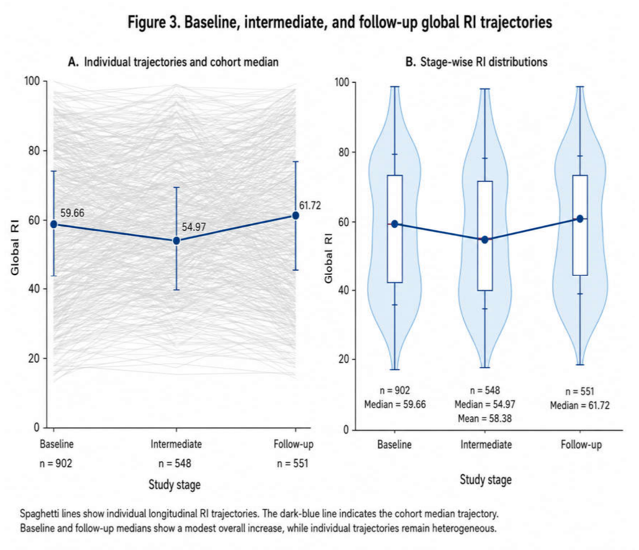
Figure 4.
Observed versus predicted global Restorative Index values across the main prediction tasks. Each panel shows cross-validated observed global RI values on the x-axis and model-predicted global RI values on the y-axis, with the diagonal identity line indicating perfect prediction. Panel A shows intermediate RI prediction. Panel B shows final RI prediction from baseline features only. Panel C shows final RI prediction using the latest known pre-follow-up RI, which produced the strongest global RI prediction performance among the main models. Panel D shows the dynamic final RI model using the latest known RI trajectory. Across panels, prediction was feasible but residual dispersion remained substantial, indicating that global RI trajectories were only partially explained by baseline, prior trajectory, treatment, dose, and timing features.
Figure 4.
Observed versus predicted global Restorative Index values across the main prediction tasks. Each panel shows cross-validated observed global RI values on the x-axis and model-predicted global RI values on the y-axis, with the diagonal identity line indicating perfect prediction. Panel A shows intermediate RI prediction. Panel B shows final RI prediction from baseline features only. Panel C shows final RI prediction using the latest known pre-follow-up RI, which produced the strongest global RI prediction performance among the main models. Panel D shows the dynamic final RI model using the latest known RI trajectory. Across panels, prediction was feasible but residual dispersion remained substantial, indicating that global RI trajectories were only partially explained by baseline, prior trajectory, treatment, dose, and timing features.
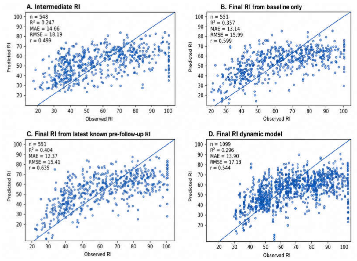
Figure 5.
Domain-specific Restorative Index model performance across biological domains and prediction tasks. The heatmap shows the best cross-validated R2 values obtained for domain-specific RI prediction models across the evaluated biological domains and modeling tasks. Warmer or higher-intensity cells indicate stronger predictive performance. Renal/uric and hematology/CBC domains showed the most consistent predictability, particularly for intermediate RI prediction and final RI prediction using the latest known pre-follow-up RI. These findings suggest that selected organ-system-specific RI trajectories may be more coherent and modelable than the aggregate global RI.
Figure 5.
Domain-specific Restorative Index model performance across biological domains and prediction tasks. The heatmap shows the best cross-validated R2 values obtained for domain-specific RI prediction models across the evaluated biological domains and modeling tasks. Warmer or higher-intensity cells indicate stronger predictive performance. Renal/uric and hematology/CBC domains showed the most consistent predictability, particularly for intermediate RI prediction and final RI prediction using the latest known pre-follow-up RI. These findings suggest that selected organ-system-specific RI trajectories may be more coherent and modelable than the aggregate global RI.
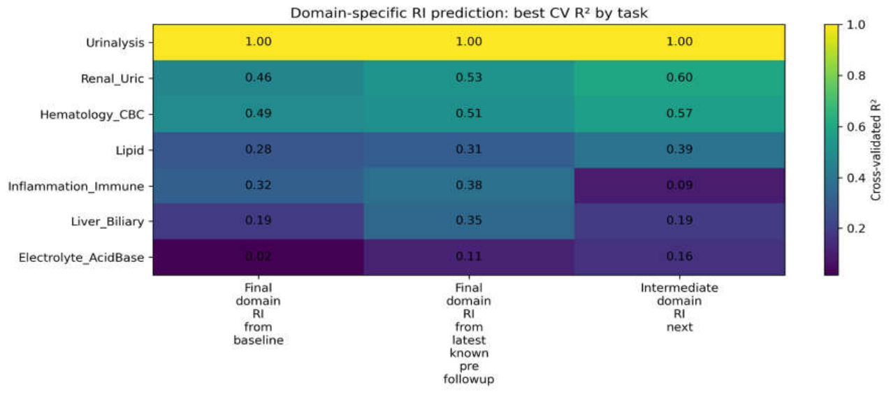
Figure 6.
Global Restorative Index estimation and prediction from domain-specific Restorative Indices. Panel A shows formula-based reconstruction of same-date global RI from domain-specific abnormality burdens and domain analyte counts. Panel B shows same-date machine-learning estimation of global RI using domain-specific RI and coverage features, representing the strongest domain-to-global estimation task. Panel C shows longitudinal prediction of final global RI from domain-specific RI dynamics. Same-date domain-specific RI profiles partially reconstructed the global RI, supporting a hierarchical RI framework, whereas future final global RI prediction from domain RI dynamics was weaker, indicating that domain-specific RIs are more useful for interpretive decomposition than for standalone prediction of future global RI.
Figure 6.
Global Restorative Index estimation and prediction from domain-specific Restorative Indices. Panel A shows formula-based reconstruction of same-date global RI from domain-specific abnormality burdens and domain analyte counts. Panel B shows same-date machine-learning estimation of global RI using domain-specific RI and coverage features, representing the strongest domain-to-global estimation task. Panel C shows longitudinal prediction of final global RI from domain-specific RI dynamics. Same-date domain-specific RI profiles partially reconstructed the global RI, supporting a hierarchical RI framework, whereas future final global RI prediction from domain RI dynamics was weaker, indicating that domain-specific RIs are more useful for interpretive decomposition than for standalone prediction of future global RI.
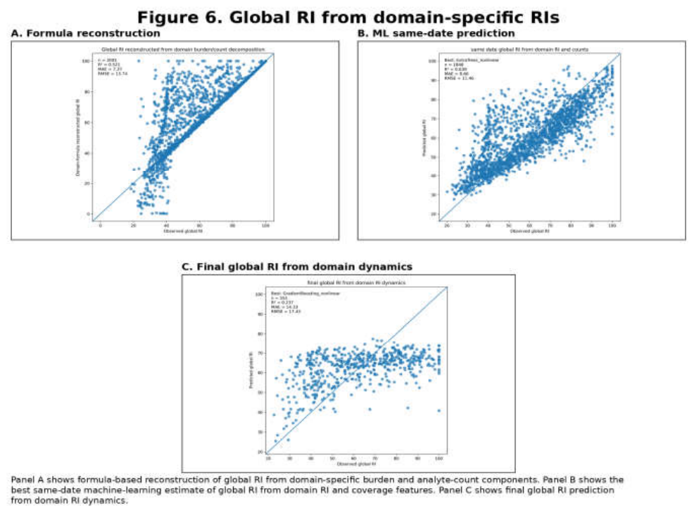
Table 1.
Dataset composition and Restorative Index panel eligibility.
| Metric | Result |
|---|---|
| Eligible subject-date panels | 2,001 |
| Subjects with baseline RI | 902 |
| Subjects with follow-up RI | 551 |
| Subjects with intermediate RI | 306 |
| Intermediate RI rows | 548 |
| RI analytes included | 62 |
Table 2.
A. Stage-wise RI summary. B. Change classification.
| (A) | ||||
| Stage | n rows/subjects | Median RI | ||
| Baseline | 902 | 59.66 | ||
| Intermediate | 548 | 54.97 | ||
| Follow-up | 551 | 61.72 | ||
| (B) | ||||
| Change category | Definition | n | ||
| Improved | ΔRI ≥ +5 | 227 | ||
| Stable | −5 < ΔRI < +5 | 167 | ||
| Declined | ΔRI ≤ −5 | 157 | ||
Table 4.
Predictive model performance for intermediate and final global Restorative Index.
| Prediction task | Best model | CV R2 | MAE | RMSE |
|---|---|---|---|---|
| Intermediate RI | XGBoost / RandomForest | ~0.246-0.247 | ~14.7 | ~18.2 |
| Final RI from baseline only | ElasticNetCV | 0.357 | 13.14 | 15.99 |
| Final RI dynamically from latest known RI | ElasticNetCV | 0.296 | 13.90 | 17.13 |
| Final RI from last pre-follow-up RI | ExtraTrees | 0.417 | 12.24 | 15.23 |
Table 5.
Predictive model performance for selected domain-specific Restorative Indices.
| Domain/task | Best model | CV R2 | MAE | RMSE |
|---|---|---|---|---|
| Renal/Uric intermediate RI | ExtraTrees | 0.598 | 11.65 | 15.16 |
| Hematology/CBC intermediate RI | ExtraTrees | 0.570 | 10.54 | 13.45 |
| Renal/Uric final RI from latest known pre-follow-up | ExtraTrees | 0.525 | 10.60 | 14.57 |
| Hematology/CBC final RI from latest known pre-follow-up | ExtraTrees | 0.510 | 11.10 | 14.24 |
| Hematology/CBC final RI from baseline | ExtraTrees | 0.492 | 11.38 | 14.57 |
| Renal/Uric final RI from baseline | ExtraTrees | 0.465 | 11.69 | 15.43 |
Table 6.
Global Restorative Index estimation and prediction from domain-specific Restorative Index features.
Table 6.
Global Restorative Index estimation and prediction from domain-specific Restorative Index features.
| Task | Best model | CV R2 | MAE | RMSE |
|---|---|---|---|---|
| Same-date global RI from domain RI only | ExtraTrees | 0.621 | 8.88 | 11.74 |
| Same-date global RI from domain RI + counts | ExtraTrees | 0.639 | 8.66 | 11.46 |
| Same-date global RI from domain RI + burden + counts | ExtraTrees | 0.636 | 8.64 | 11.51 |
| Final global RI from baseline domain RIs | GradientBoosting | 0.211 | 14.71 | 17.72 |
| Final global RI from latest pre-follow-up domain RIs | GradientBoosting | 0.226 | 14.57 | 17.55 |
| Final global RI from domain RI dynamics | GradientBoosting | 0.237 | 14.33 | 17.43 |
Disclaimer/Publisher’s Note: The statements, opinions and data contained in all publications are solely those of the individual author(s) and contributor(s) and not of MDPI and/or the editor(s). MDPI and/or the editor(s) disclaim responsibility for any injury to people or property resulting from any ideas, methods, instructions or products referred to in the content. |
© 2026 by the authors. Licensee MDPI, Basel, Switzerland. This article is an open access article distributed under the terms and conditions of the Creative Commons Attribution (CC BY) license (http://creativecommons.org/licenses/by/4.0/).
Copyright: This open access article is published under a Creative Commons CC BY 4.0 license, which permit the free download, distribution, and reuse, provided that the author and preprint are cited in any reuse.


