
Submitted:
07 July 2026
Posted:
09 July 2026
You are already at the latest version
Abstract
This paper presents the application of artificial intelligence, gaming, and optimization algorithms to safe route planning and traffic control for various types of autonomous vehicles. The study covers autonomous mobile robots and vehicles based on land, autonomous surface and underwater vehicles based in water, marine autonomous surface ships, and autonomous air vehicles. Biomimetic autonomous vehicle solutions are presented for each of these three areas of operation. A comparative analysis of the methods enables the mapping of real-world characteristics of autonomous processes, such as their multi-objective and game-like nature. To address the challenges of ensuring the safe operation of autonomous systems, this work presents a comparative assessment of individual route-planning methods regarding collision risk and optimality. In particular, route-planning methods are developed for various possible kinematic, dynamic, and game trajectories, both cooperative and non-cooperative. An experiment comparing individual path-planning methods was conducted using examples of recorded real-world navigation situations. Following the analysis, special attention was paid to the types and methods of cybersecurity used for individual types of autonomous vehicles.
Keywords:
autonomous vehicles
; biomimetic objects
; artificial neural network
; linear and dynamic programming
; game theory
; planning algorithms
; cybersecurity
1. Introduction
The effectiveness of real autonomous vehicle deployment depends on safely completing the planned route. This success depends on the efficiency of the vehicle’s drive, motion sensor hardware, and functional software and, in particular, planning the best, safest trajectory. We can choose between dangerous and safe trajectories, but only one can be optimal. Route-planning strategies for autonomous systems take into account physical constraints, environmental hazards, and freedom of movement. Airborne and waterborne vehicles operate in large three-dimensional spaces, while land vehicles navigate limited two-dimensional road networks with nonholonomic kinematics and dynamic local traffic. Venu S. and Gurusamy M. [1] examined route planning in a much broader context than robotics and autonomous vehicles, encompassing urban mobility, healthcare robots, search-and-rescue operations, logistics, and warehousing. In urban mobility, route-planning algorithms improve traffic flow and optimize route planning in smart cities, and in healthcare, they help surgical robots to navigate precisely in constrained environments. Autonomous air vehicles (AAVs) and mobile robots (AMRs) can maneuver through hazardous or disaster-stricken zones during search-and-rescue operations, and can also perform logistics route planning to automate the rapid delivery of goods in dynamic warehouse environments. For these applications, route-planning algorithms must evolve continually throughout their design and operation. A combination of more advanced computational processes, sensor technologies, and artificial intelligence-based technologies is essential. Such approaches hold enormous promise, as they are transforming the way autonomous devices interact with and navigate the world. Fossen T.I. et al. [2] emphasize that guidance, navigation, and traffic control systems for autonomous vehicles are increasingly important in land, sea, and air operations. Autonomous underwater vehicles can be used for pipeline inspection, light intervention work, underwater research, and oceanographic/biological data collection. Autonomous unmanned aerial systems can be used in many applications, such as inspection, monitoring, data collection, and surveillance. Currently, vehicles operate with limited autonomy and minimal intelligence. There is a growing interest in cooperative and coordinated multi-vehicle systems, real-time replanning, robust autonomous navigation systems, and robust autonomous vehicle control. Unmanned vehicles with a high level of autonomy can be used to safely and efficiently collect environmental data, assimilate climate and environmental models, and complement global satellite systems.
The aim of this work is to demonstrate that by utilizing select methods from automatic control theory, artificial intelligence, and game theory, it is possible to develop algorithms for determining safe trajectories for various types of autonomous vehicles that will ensure optimal performance of their tasks.
The main achievements of this work include:
- The development of algorithms for determining safe trajectories for kinematic, dynamic and game-cooperative and non-cooperative land, water, and aerial vehicles.
- The application of methods of assessing the optimality of safe trajectories in the context of collision risk and deviation from the reference route.
- Accounting for environmental conditions by assigning appropriate collision risk models.
The rest of this paper is organized as follows: Section 2 contains a review of the literature on the topic of this work. Section 3 describes the necessary theoretical tools in the areas of control techniques, optimization, artificial intelligence, and game theory. Section 4 and Section 5, and 6 present algorithms for determining the safe trajectories of autonomous land, water, and aerial vehicles, respectively, as well as relevant cybersecurity and biomimetic solutions. The experimental results are discussed in Section 7, indicating the advantages and limitations of individual methods for determining safe vehicle trajectories. Finally, Section 8 presents the most important conclusions of this research and a plan for further investigation.
2. Related Work
2.1. Autonomous Land Vehicles
Autonomous ground vehicles, including mobile robots and self-driving cars, operate on well-defined roadways or in open environments while navigating around static and dynamic obstacles such as pedestrians and other vehicles. Key challenges they face include stringent kinematic limitations—such as turning radius constraints and restricted lateral movement—alongside the need for real-time detection and avoidance of obstacles, as well as varying levels of traction with the ground. Path planning is a critical aspect of mobile robot functionality, serving as the basis for addressing several related navigation issues. The authors of [3] indicate that the complexity of path planning escalates with an increase in the size and quantity of obstacles present within a given area, impacting the choice of suitable planning techniques. A thorough review of research on autonomous mobile robots is warranted, including various subjects such as sensor types, mobile robot platforms, simulation tools, path-planning and tracking strategies, sensor fusion techniques, and obstacle avoidance methods [4]. For instance, the authors of [5] proposed a three-tier framework for managing unmanned cargo transport systems in seaports and discussed difficulties linked to implementing route-planning and traffic management technologies for autonomous freight vehicles operating in port settings. The task of autonomous driving in unpredictable environments—including agriculture, military operations, and mining contexts—demands a comprehensive hierarchical approach to route planning [6]. A comparative analysis, presented in [7], was conducted on widely used route-planning algorithms tailored to unstructured terrains such as forests and mountainous areas. Methodologies catered toward autonomously exploring and mapping unknown surroundings are vital components of route-planning endeavors [8]. An extensive examination of decision-making and planning algorithms relevant to autonomous driving is crucial. This includes knowledge-based methods—which use systems driven by rules, state transitions, or game theory—and autonomous planning strategies that encompass search-based techniques, sampling approaches, and optimization practices [8]. There are also data-driven tactics involving machine learning frameworks such as imitation learning, reinforcement learning, and inverse reinforcement learning [9]. The earliest patents concerning route planning for autonomous vehicles are also significant in this context [10,11].
2.2. Autonomous Water Vehicles
Autonomous surface vehicles (ASVs), underwater vehicles (AUVs), and ships navigate in a three-dimensional space that is constantly subject to changing natural forces. Key challenges include the influence of sea currents, wind, and waves; extended braking distances; and compliance with regulatory frameworks such as the International Maritime Organization's Convention on the International for Preventing Collisions at Sea (COLREGs). Deep reinforcement learning has shown significant potential for collision avoidance in unmanned surface vehicles. To address these challenges, the authors of [12] introduce an ASV collision avoidance strategy using Gaussian-distributed actor–critic mixed models. In [13], trajectory tracking and collision avoidance for ASVs in the context of maritime sports support are analyzed. An adaptive control strategy with a predefined gliding mode was proposed to manage tracking errors of the CyberShip II-based ASV system. The review presented in [14] categorizes the variety of path-planning algorithms found in the existing literature on unmanned ships and sailboats, examining their advantages, disadvantages, and evaluation metrics. Ref. [15] presents a compliance framework based on COLREGs. Traditional approaches to autonomous ship navigation in grid-based maritime environments require discretization, which dictates path resolution based on area scale and spatial complexity. In wide geographic regions, this resolution may not be able to satisfy complex navigation requirements, leading to suboptimal or inaccurate routing. To address this problem, the authors of [16] proposed a parameterized path-planning algorithm that represents navigation areas and obstacles using polygons derived from electronic navigation charts rather than discrete grids. The review presented in [17] evaluates route-planning algorithms used by autonomous maritime autonomous surface ships (MASSs) in the context of collision regulation to illustrate how researchers address these challenges. The results suggest that route-planning algorithms should consider various traffic regulations; particularly those that can be fine-tuned for safe distance parameters or constraints. Effective collision avoidance technology is crucial for AUVs operating in aquatic environments. Many existing electrical impulse measurement techniques rely on fixed static thresholds, which limit adaptation to external dynamic changes. In [18], a bio-inspired approach was proposed, which is characterized by dynamic adaptive thresholds modeled based on temporal changes in biological neural systems. This method combines spiking neural networks with deep reinforcement learning tailored to AUV operations involving dynamic underwater collision avoidance tasks in complex, unknown environments. Regarding UAV route-planning methodologies, common strategies include graph search routing, optimization processes, and particle swarm intelligence techniques [19].
2.3. Autonomous Aerial Vehicles
Unmanned aerial vehicles operate in open, three-dimensional spaces that have the lowest density of static ground obstacles but are highly dynamic due to variable air currents. The main challenges in these contexts are limitations resulting from flight dynamics—minimum speed, ceiling, airspace restrictions, geofencing—and high energy consumption during take-off maneuvers. In [20], a two-stage cooperative encirclement model for autonomous aerial devices (AAVs) was proposed, consisting of an acquisition phase and a homing phase. In the acquisition phase, an error-correcting polynomial interpolation and fitting method is developed to achieve early capture and significantly improve the accuracy of intruder trajectory prediction. For capture point allocation, an iterative allocation strategy based on convex optimization is developed to minimize the total energy consumption of the system while strictly satisfying the capture formation constraints. According to [21], a fundamental aspect of AAV autonomy is route optimization, which determines efficient paths by taking into account factors such as mission objectives, safety, and energy consumption. AAV route-planning methodology involves deterministic models, stochastic sampling techniques, bioinspired methods, and integrated algorithmic frameworks. To improve the competitiveness of AAV logistics compared with traditional ground logistics, a two-layer route network structure was constructed [22] that separates logistics transshipment from terminal delivery. In the delivery layer, a door-to-door distribution metod was adopted, and a model was established to identify the locations of transshipment nodes their associated service connections. In the transshipment layer, a standard index for deviation between routes was introduced to construct a route-network-planning model. A two-layer algorithm was designed to solve this above model.
2.4. Cybersecurity
The reduced human involvement in autonomous systems compared with traditional non-autonomous systems increases the impact of cyberattacks because humans have fewer opportunities to detect, intervene, or mitigate malicious activity. Research has explored the vunerabilities of autonomous systems – such as sensing communication, and navigation – in specofic applications like Autonomous Surface Vehicles (ASVs) and Autonomous Aerial Vehicles (AAVs). Furthemore various studies have focused on defence mechanisms designed to prevent, detect, and mit9gate thesse vulnerabilities. For example, some defensive approaches utilize redundancy and cross-validation technicues to recgnize compromised sensor data or implement localization strategies that combine multiple postioning systems to counter spoofing or jamming attacs [23]. The open-source nature of AAV software and protocols heightens their vunerability resulting in a growing array of cybersecurity challenges. An evaluation of AAV architecture clasifies security treats into four main categories: communication network, software, payload, and intelligent security [24]. The authors of [25] concluded that it is essential to model autonomous systems from a security perspective, identify threats and vulnerabilities, and then model attacks. This review examines analytical models of systems and attacks and identifies a research gap that the scientific community needs to fill.
3. Theoretical Tools
Theoretical tools for controlling autonomous objects encompass a wide range of mathematical and engineering methods that enable robots and vehicles to make decisions and complete tasks independently. Among the most important are control techniques, optimization, artificial intelligence, and game theory.
3.1. Control Techniques
Real-time control algorithms utilize microcontrollers or programmable logic controllers (PLCs) to monitor and directly control autonomous objects digitally. Adaptive control is an advanced feature often implemented within direct digital control.
In a direct digital control system (DDC), the controlled variable is converted into a digital signal at discrete moments in time and then, according to the programmed control algorithm in the PLC, is converted into a setting signal (Figure 1).
The incremental proportional–integral–derivative (PID) direct digital control algorithm used to control actuators of autonomous objects operates according to the following relationship:
The algorithm settings comprise the following parameters:
- Gain coefficient KP;
- Integral coefficient KI;
- Derivative coefficient KD.
The following types of adaptive control are distinguished:
- Gain scheduling (GS) controller tuning;
- Model reference adaptive system (MRAS);
- Self-tuning regulator (STR).
During adaptive control, functions to identify the dynamics of the autonomous object and tuning are implemented as appropriate changes in the PID controller settings.
3.2. Optimization
Autonomous system optimization means achieving maximum effect without any human input while preserving full safety and resource constraints. The process is based on the combination of mathematical computational modeling and optimal control theory. The optimization tools used are as follows:
- Linear programming;
- Dynamic programming;
- Linear quadratic regulators (LQRs);
- Model predictive control (MPC);
- Linear matrix inequalities (LMIs).
3.3. Artificial Intelligence
For automatic vehicles and robots, artificial intelligence systems allow them to operate autonomously, cope with ever-changing surroundings, and make decisions freely and without human intervention.
An artificial neural network is a computational system whose layout and behavior is based on the human body’s nervous system. The most useful advantage of neural networks is their capability to learn and adapt without an exact understanding of the method applied to control the autonomous object. In this way, a neural network can learn to autonomously respond to input and output signals to complete certain tasks.
Fuzzy control is a fuzzy-logic-based control method applied in automatic systems and robotics. Fuzzy logic, unlike classical logic, allows for intermediate values between 0 and 1 and facilitates decision-making under uncertain (or imprecise) circumstances. Fuzzy control is utilized in autonomous systems that are mathematically difficult to describe yet require precise operation. It has some advantages, such as a high immunity to interference and the ease of implementing expert knowledge—a human frame of mind—in the algorithm guiding the autonomous object.
An evolutionary algorithm, relative to deterministic optimization methods, undertakes a search that begins not from a single point but from a range of points and applies probabilistic, not deterministic, rules to select the optimal solution.
An expert system is a computer program in the realm of artificial intelligence that is capable of automating the decision-making process of a human expert in a highly specific and specialized field. It is based on knowledge that is stored in the system—rules, facts and reasoning procedures—that makes it feasible for an autonomous robot to carry out complex operations.
Particle swarm algorithms exploit a population of moving particles to search for an appropriate fitness function, such as the control objective function. These particles can learn a point in the search space by memorization, a process in which the desired objective function has the greatest value, and transmit that to all or a fraction of the population. Individual particles that have learned from this information can change their position to reach the point with the maximum value.
A multi-agent system is a distributed computer system comprising a large number of interacting elements, such as agents. It is not a central program that performs all the processing; it is a group of independent entities that communicate to solve problems better, than a single agent can. Every agent is independent, with its own goals, and makes decisions without constant external supervision. Agents share information, trade, cooperate, and opportunities to learn and, under certain circumstances, compete.
Machine learning is a form of artificial intelligence (AI) in which computers learn on their own without executing a programmed action on a sequential basis. Instead of static rules, algorithms process massive quantities of information, identify recurrent patterns in the data, and develop a mathematical model that can be used by a given autonomous object to make predictions or decisions.
3.4. Game Control
Game-theoretic methods of control, particularly of autonomous objects, are used to model interactions between multiple autonomous objects or between the controller of an autonomous object and an uncertain environment, seeking to determine the players’ strategies. The largest class of games that can be applied to the play-based control of autonomous objects are differential games which, in their extensive form as multi-step games, take the form of matrix and positional games.
In a matrix game, the first player, as their own autonomous object, can use various pure strategies, and the second player, as an autonomous object the first player encounters, can also use a variety of pure strategies. Such a game is described using a collision risk matrix, where the number of rows corresponds to the number of permissible strategies of the first-player autonomous object, and the number of columns consists of the total number of permissible strategies of all the autonomous objects involved in a given collision situation.
The role of a positional game in an autonomous system is to make the strategy of the first-player object in the present step dependent on the positions of the objects it encounters. This allows the process model to account for any changes in the course and speed of the objects encountered while executing control. The criterion for selecting the optimal trajectory of the first-player object is to determine its course and speed, ensuring the smallest distance losses for safely navigating around objects encountered in a distance no smaller than the assumed value, taking into account the dynamics of the object in the form of the lead time of the maneuver.
4. Autonomous Land Vehicles
Autonomous land vehicles can be autonomous mobile robots or autonomous vehicles (AVs); they employ intelligent technologies such as sensors, cameras, radars, LiDAR (Light Detection and Ranging), and artificial intelligence for autonomous mobility. Environmental sensors obtain real-time data and evaluate it using AI algorithms that inform decision-making. These sensors record distances and detect objects surrounding the vehicle (using radar and LiDAR), enabling navigation under dynamic road conditions. A GPS device provides location information, and computer vision is employed to recognize traffic signals and other road users.
4.1. Autonomous Mobile Robots
With their efficiency and ability to cover diverse ground, AMRs are utilized in automation, logistics, and exploration. Their wheeled or tracked shape permits rapid and agile movement, making them suitable for various technological applications (Figure 2).
Mobile robot motion planning consists of path planning and trajectory planning. Path planning and trajectory planning are two consecutive stages of a mobile robot’s navigation process—the first is determines where the robot is going, and the second determines how it will get there.
4.1.1. Path Planning
Robot path-planning methods involve finding a sequence of points or path sequences along which the robot will move to reach its destination from the starting point while avoiding collisions with obstacles and taking into account a given quality criterion (objective function); for example, the shortest, fastest, or least energy-intensive path.
Mobile robot path planning is implemented using a variety of methods.
-
Global methods:
- –
- A* heuristic algorithm;
- –
- Dijkstra’s algorithm;
- –
- Wave propagation;
- –
- Voronoi diagram;
- –
- Visibility graph.
-
Local methods:
- –
- Potential fields;
- –
- Elastic ribbon.
-
Artificial intelligence methods:
- –
- Evolutionary algorithm;
- –
- Ant colony algorithm;
- –
- Expert algorithm;
- –
- Machine learning.
4.1.2. Trajectory Planning
Trajectory planning involves determining how the robot should move along a designated path. This involves timing, taking into account the robot’s dynamics and kinematics, as well as constraints such as its maximum velocity, acceleration, and other dynamic parameters of the path (Figure 3).
The current status of the collision avoidance process for multiple autonomous mobile robots is monitored using measurement devices such as radar, gyroscope, logger, LiDAR, and GPS.
Computational intelligence algorithms for the safe trajectory of the autonomous mobile robot constitute a significant part of the system and include a neural network with dynamic programming and a cooperative and non-cooperative risk game. For the purpse examined.
The process model envisions a multi-stage implementation for robot control, transitioning from the initial state to the final state. The final state is achieved by safely navigating around all encountered robots and reverting to theoriginal path. The dynamics of the robot are facrored in by considering the lead time required for maneuvering corse adjustments, which roughly corresponds to the values of threee time constants associatedd with the robot.
Individual algorithms differ in their approach to formulating the control objective function, ranging from not taking into account changes in the courses and speeds of the encountered robots (kinematic trajectory (KT) algorithm) to assigning the encountered robots domains generated by an artificial neural network (dynamic trajectory (DT) algorithm), or the game trajectory (GT) algorithms that consider the cooperative (GT_c) and non-cooperative strategies (GT_nc) of the encountered robots.
Kinematic Trajectory (KT) Algorithm
The KT algorithm does not contain artificial intelligence elements and is used for comparison with the dynamic and game algorithms (Figure 4).
It is assumed that the encountered robot j moves with a constant heading ψj and velocity Vj. The basis for determining safe robot trajectories via synthesizing algorithms is to first determine the allowable sets of course and/or velocity changes that ensure safe passage of the robot.
Robot 0, moving at speed V0, heading ψ0 at a distance Dj, and bearing Nj relative to the encountered robot j moving at speed Vj and heading ψj, should pass it at a safe distance Ds. To achieve this, there are infinitely many possible course and velocity changes from the set of allowable maneuvers to the left side of L0 or to the right side of R0. The optimal solution, which ensures the maximum projection of the velocity vector in the given direction of the robot’s movement and leads to the smallest trajectory losses while safely passing the encountered robots, is selected from this set.
The optimization criterion is the smallest distance loss necessary to safely pass all j robots; this is achieved with the maximum projection of the robot’s velocity vector V0 in the x direction of its movement to the nearest turning point on the given movement route:
The minimum-time criterion (2) achieves the safe passing distance Ds by first changing the robot’s heading 0 to the value to port or to starboard in a manner that satisfies the priority rule. If this is not possible, the algorithm decides to reduce the speed to the value .
Simplex linear programming was used to optimize this control problem, which limits the possible solutions in the linear sets P0 and S0 and allows for determining the optimal solution ensuring the minimum control quality index (2).
Dynamic Trajectory (DT) Algorithm
The DT algorithm takes into account the degree of danger caused by the movement of passing robots j at each step k when calculating the safe trajectory of robot 0 by assigning them a hexagonal domain, the size of which is shaped by a previously trained artificial neural network (Figure 5).
To assess the collision risk with robot j, a unidirectional neural network comprising three layers is employed. This nework featuers six neurons in the input, three in hiden, an one in output layers. Neurons within both the input and hiden layers apply a hyperbolic tangent activation function, while the neuron in the output layer a sigmoidal unipolar activation function.
The task of identifying an optimal trajectory for robot 0 involves selecting from numerous viable safe paths that do not infringe upon defined neural regions indicating potential collisions with robot j. This selection process is approached as a multi-stage decision-making procedure. The Bellman dynamic programming method and the time-optimal optimization criterion are used to solve this process:
Game Trajectory (GT) Algorithm
The GT algorithm considers the collision risk by formulating a multi-object matrix game model. The collision risk rj is formulated as a function of the minimum distance and the time for robot j to pass robot 0 and the distance Dj between them:
In addition to the previously mentioned robot approach parameters, the collision risk value depends primarily on the course- and speed-changing maneuvers performed by the robots; i.e., the game control strategy (Figure 6).
A collision risk matrix is created in which the number of rows corresponds to the number of maneuvering strategies of robot 0, and the number of columns corresponds to the maneuvering strategies of individual robots j.
Therefore, the optimization criterion in a cooperative matrix game will be as follows:
In a non-cooperative matrix game, the form is as follows:
Figure 7 illustrates a comparison of safe trajectories of the autonomous robot passing eight other robots, determined according to the individual algorithms KT, DT, GTc, and GTnc.
4.1.3. Motion Control
The following types of algorithms are used to control the motion of holonomic robots:
- Basic—PID algorithms;
- Learning—neural network algorithms;
- Accounting for uncertainty—fuzzy logic algorithms.
The following types of algorithms are used to control the movement of non-holonomic robots:
- Basic—PID algorithms;
- Optimization—LQR algorithms;
- Prediction—MPC algorithms.
4.1.4. Cybersecurity for Autonomous Mobile Robots
For AMRs, cybersecurity comprises a set of technologies, processes, and practices designed to protect robots, their software, data, and the networks they operate on from unauthorized access, cyberattacks, and manipulation. AMRs are intelligent, networked machines that utilize LiDAR sensors, cameras, and AI to navigate uncontrolled environments. Due to their connectivity, they are potential targets for attacks by agents resembling a mobile insider within a company’s IT infrastructure.
Threats to AMRs include the following:
- Hijacking;
- Industrial espionage;
- Network intrusion;
- Data manipulation.
AMR cybersecurity strategies include the following:
- Encrypted communication;
- Secure booting;
- Access control;
- Software updates;
- Compliance with industry standards for automation system security.
4.2. Autonomous Vehicles
AVs are vehicles that can drive themselves with minimal or no human intervention. Their operation relies on advanced systems that allow them to navigate, accelerate, brake, and avoid obstacles (Figure 8).
The following are AV perception and localization algorithms:
- Global positioning systems;
- Inertial measurement unit;
- Simultaneous localization and mapping;
- Image recognition.
AV control algorithms integrate sensor data to make decisions and control the vehicle’s movement in real time.
Figure 9 illustrates the hierarchical structure of the control system in a group of autonomous vehicles.
4.2.1. Trajectory Planning
With respect to trajectory planning for autonomous vehicles, the following types of trajectories can be distinguished:
- Kinematic trajectory, which takes into account vehicle dynamics in the form of lead time for course or speed changes;
- Dynamic trajectory, which takes into account vehicle dynamics in the form of process state equations;
- Game trajectory, which takes into account possible course and speed changes of other autonomous vehicles (Figure 10).
Kinematic Trajectory (KT)
In a multi-stage approach, the KT algorithm takes into account the kinematic equations of autonomous vehicles, corresponding to the sequence of subsequent maneuvers.
The optimal collision avoidance maneuver, which allows the vehicle to maintain the previously established safe passing distance ds by optimally changing the course to the right χ*0,r or left χ*0,L or optimally reducing the speed σ0*, is determined from the area of permissible maneuvers (green), the structure of which is shown in Figure 11.
The Simplex linear programming method is used to calculate optimal course and speed values within a limited area of allowable maneuvers. The criterion for optimal vehicle control quality is reaching the nearest turning point with the smallest distance loss during the anti-collision maneuver. These losses are lowest at the maximum vehicle speed component in the direction leading to that turning point along the given trajectory. When the vehicle moves at a constant speed, minimizing the distance loss s* is equivalent to minimizing the time t* needed to reach the autonomous vehicle’s turning point on the given route:
The effect of minimizing the maneuvering time while avoiding vehicle collisions is the deviation δ* of the safe trajectory from the set trajectory, determined from the calculated optimal trajectory.
Dynamic Trajectory (DT)
The DT algorithm is based on a dynamic model of the control process, which contains state equations describing the dynamic properties of the autonomous vehicle and constraints in the form of motion domains assigned to each autonomous vehicle encountered. The circular and hexagonal domains are created by a pre-trained three-layer neural network with tangentoidal and sigmoidal activation functions. The neural network is designed using MATLAB 2026 Neural Network Toolbox software, and an error propagation algorithm with an adaptive learning rate and momentum is used for training.
The criterion for the quality of vehicle control is the smallest deviation of the route s from the nearest turning point on the route, achieved with the shortest time to reach this point:
Game Trajectory (GT) Algorithm
The GT algorithm is determined based on a multi-step positional game model for a group of autonomous vehicles.
The algorithm first determines the area of permissible maneuvers for the target autonomous vehicle relative to the other n autonomous vehicles, using the method presented in Figure 11. Then, using the same method, sets of permissible maneuvers are determined for each of the n autonomous vehicles relative to the primary autonomous vehicle. The dynamics of the autonomous vehicles are considered in terms of the maneuver lead time.
The control quality criterion is the smallest deviation of the driving path from the predetermined nearest turning point on the given route. In the case of cooperation between vehicles (algorithm GTc), this is given by
In the case of non-cooperative maneuvering (algorithm GTnc), it is
Figure 12 compares the trajectories of autonomous vehicles in multidirectional and one-way traffic, determined according to the KT, DT, GTc, and GTnc algorithms.
A comparison of the values of the final deviation of the trajectories δ* from their initial values for autonomous vehicles in multidirectional and one-way traffic depending on the safe passing distance δ for the KT, DT, GTc, and GTnc algorithms is shown in Figure 13.
4.2.2. Cybersecurity for Autonomous Vehicles
AV cybersecurity comprises a set of processes, technologies, security measures, and best practices designed to protect the electronic systems, software, communication networks, and data of modern vehicles from unauthorized access, digital attacks, and manipulation.
Cyberattacks on autonomous vehicles are classified as follows:
- Cyberattacks on electronic control units (ECUs).
- Cyberattacks on the in-vehicle network of AVs consist of the deliberate breach, disruption, or takeover of a vehicle’s information systems through access to its internal communication network. Attacks can target the engine, brakes, or steering system.
- Cyberattacks on the Keyless Entry/Go system using advanced electronic tools.
- Cyberattacks on sensors, disrupting the operation of vehicle perception and artificial intelligence systems.
- Cyberattacks on mobile apps used to monitor, lock, unlock, and remotely control vehicle functions.
- Cyberattacks on a vehicular ad hoc network (VANET), preventing vehicles from communicating vehicle-to-vehicle (V2V) and vehicle-to-infrastructure (V2I).
- Cyberattacks on the infotainment system and Bluetooth, which act as a barrier to the vehicle’s internal CAN bus network, allowing hackers to remotely take control of the vehicle.
4.3. Autonomous Biomimetic Land Vehicles
The design of autonomous biomimetic vehicles draws inspiration from nature regarding structure, behavior, or ecosystems to produce more efficient, sustainable, and intelligent systems capable of autonomous movement in various environments (Figure 14).
Biomechanical engineering is the foundation of biomimetic vehicle design; it has applications such as the following:
- Locomotion systems, where walking robots mimicking geckos, insects, or animals can navigate uneven, complex surfaces, including in disaster contexts such as rescue missions and nuclear waste disposal.
- Aerodynamic efficiency, where vehicle designs in trains, airplanes, and submarines incorporate shapes inspired by, among other things, the beak of a kingfisher, reducing air resistance and noise.
- Military and specialized applications, such as biologically inspired unmanned ground vehicles (UGVs), resembling a dog, are used in military and reconnaissance missions, minimizing risk to humans.
- Sensor cleaning for autonomous vehicles, mimicking the swinging motion of mammals shaking off water.
- Robots inspired by insects and arthropods, exhibiting biologically inspired features;
- Robots inspired by snakes, capable of navigating tight spaces and climbing complex surfaces.
5. Autonomous Water Vehicles
Autonomous water systems are technologies that can operate autonomously or remotely, without constant human supervision, to perform tasks on or under water:
- ASVs, which are capable of operating without a crew on board and used for research, monitoring, inspection, and patrol;
- Maritime autonomous surface ships;
- AUVs, operating underwater without a pilot or cable connection and autonomously carrying out pre-programmed missions such as seabed mapping, industrial monitoring, and wreck searches.
5.1. Autonomous Surface Vehicles
Autonomous surface vehicles are used in the following:
- Hydrography and surveying, for scanning the seabed, collecting bathymetric data, and monitoring the aquatic environment;
- Military operations, acting as mine-sweeping platforms, conducting reconnaissance and patrol operations, and increasing the safety of ship crews;
- Scientific research, for collecting water samples, monitoring water quality, and observing oceanographic phenomena;
- Transport and logistics, for autonomous cargo transport in ports or on short sea routes;
- Security and surveillance, for monitoring maritime borders, critical infrastructure, and search and rescue operations (Figure 15).
The control process for a group of autonomous surface vehicles, where the target autonomous vessel 0, located at position (X0, Y0), avoids collisions by changing course ψ0 as control u0, and the remaining k autonomous surface vehicles, each located at position (Xk, Yk), controlled by their course ψk as control uk, is illustrated in Figure 16.
Controlling individual vehicles influences their relative motion and the distance over which they pass each other, which determines whether a model considers cooperative or non-cooperative game. If vessels adhere to the COLREGs, the game is cooperative. However, challenging environmental conditions, interference with autonomous vehicle motion data measurements, and various subjective factors lead to a non-cooperative game (Figure 17).
The control objective function, as an index of optimal control quality, takes the form of the collision risk rk in the process of safely controlling an autonomous surface vehicle:
where is the shortest passage time of the primary vehicle and vehicle k; Ts is the safe passage time of the vehicle depending on the traffic conditions.
5.1.1. Trajectory Planning
The autonomous surface vehicle 0 has control , where i = 1, 2, …, I is the number of strategies by which it can change its course o perform an anti-collision maneuver when passing other vehicles at a distance no less than Ds. Similarly, the k vehicle uses control , where j = 1, 2, …, J is the number of strategies with which it can change its course in order to perform an anti-collision maneuver (Figure 18).
Game Trajectory (GT) Algorithm
The surface vessel’s trajectory algorithm for the GT involves creating a collision risk matrix , where the collision risk rk is a relative measure of safety when vehicles pass each other. The current situation is described by the values . The safe situation is defined by the quantities (Ds, Ts). Collision risk rk is defined as the mean squared measure of the relationship between the assessment of the current situation and the proximity of vehicles to the expected safe situation, as follows:
where cd, ct, and c are weighting factors that depend on traffic conditions, taking values from 0 to 1. For example, in situations of concentrated vehicle traffic, cd = ct = 0.4, c = 0.5, and in situations of greater distances between vehicles, cd = ct = 0.5, c = 0.1.
The GTnc algorithm calculates the elements of the collision risk matrix, where the number of rows is equal to the number of strategies of the primary vehicle and the number of columns is equal to the total number of strategies of all other vehicles.
The safe and optimal trajectory of the primary vehicle 0 in a group of k other vehicles is calculated using dual linear programming:
It is assumed that for various unknown reasons, k other vehicles will collide using strategy j, which maximizes the collision risk. Next, the primary vehicle, for this strategy of the other vehicles, determines acceptable strategies, from which it selects strategy i, which minimizes the collision risk by executing an anti-collision maneuver.
Kinematic Trajectory (KT) Algorithm
Assuming that other vehicles move without changing their course over time, the game control task reduces to a non-game control task:
Figure 19 shows the safe game and non-game trajectories of the primary vehicle among the group of k = 14 other vehicles, determined by the GTnc and KT algorithms.
5.1.2. Cybersecurity for Autonomous Surface Vehicles
Cybersecurity for ASVs, including protection against remote hijacking, is a key aspect of their operability. Given the growing role of underwater ASVs in protecting ports and offshore wind farms, their reliability directly depends on their resistance to cyberattacks, which can lead to environmental disasters, technology theft, or collisions.
The following are cyber threats to ASVs:
- GNSS/GPS spoofing—the most serious threat, involving the transmission of false location signals, allowing a hacker to alter the vessel’s course, drive it aground, or hijack it.
- Signal jamming—jamming radio/satellite communications, which cuts the USV off from its shore-based operator, preventing remote control.
- Denial of service/distributed denial of service (DoS/DDoS) attacks—overloading the vessel’s communication systems, leading to its immobilization or loss of control.
- Man-in-the-middle (MMA) attacks—interception of communication between the control station and the ASV, enabling the injection of false commands.
- Software attacks (malware/firmware)—infecting operating systems with malware, which can lead to the theft of sensitive data, such as maps and research results, or sabotage.
- IS system vulnerabilities—manipulating data from the automatic identification system (AIS), which distorts the situational awareness of other vessels.
- The following are methods of protecting ASVs from cyberattacks:
- Communication encryption—use of advanced encryption algorithms for all data transmitted between the ASV and the SCC.
- Authentication—implementation of strong authentication mechanisms to prevent unauthorized devices from accessing the USV network.
- Security by design—considering cybersecurity issues at the design stage of the units, not only during their operation.
- Intrusion detection systems—implementation of systems that monitor traffic in the onboard network and detect unusual behavior; for example, using machine learning.
- System hardening—regular firmware updates and removal of vulnerabilities in control systems.
5.2. Autonomous Ships
MASSs are surface vessels that can operate with minimal or no crew. This means there is no need for humans on board, which can significantly reduce operating costs and increase the efficiency of maritime transport. The development of autonomous ships is aimed at improving safety at sea and protecting the environment. Reducing the number of people on board not only minimizes the risk of accidents but also allows for more precise management of resources and emissions (Figure 20).
The MASS vessel traffic control process includes functions such as automatic steering along a preset course or trajectory, collision avoidance, optimal route navigation, and precise control during port entry, berthing, and anchoring. The systems performing these functions are closely interconnected and form a hierarchical, multi-level MASS vessel traffic control system (Figure 21).
The structure of this multi-layer system is governed by a hierarchy of control modes. First, an optimal voyage route is determined. Then, as the ship moves along this route, if collision avoidance is necessary, a safe trajectory to the nearest turning point on the optimal route is determined. The ship’s movement along each segment is controlled directly in real time.
5.2.1. Route Optimization
To determine the optimal route (OR) for a MASS, an evolutionary algorithm is used to route the vessel, in which each individual in the population represents a potential solution to the problem. During the calculation, the algorithm operates on a population of individuals representing different variants of the vessel’s route, described by a polygonal line with constant speeds along each route segment. The route representation in the evolutionary algorithm includes an ordered set of turning points in the form of their geographic coordinates, with an additional parameter describing the speed along the route segment between successive points.
The optimization criterion is
where Qt is the total route cost, Qs is the route safety cost, and Qe is the route economic cost.
The route safety cost Qs increases proportionally with a decrease in distance between the ship and constraints, static and dynamic. The economic cost Qe is proportional to the time and fuel (energy) required to traverse a given route (Figure 22).
5.2.2. Trajectory Planning
The process of controlling the movement of an autonomous MASS first involves determining a safe and optimal trajectory and then steering it along that trajectory. In a navigational situation at sea, there are various possible methods of controlling the movement of an autonomous ship (Figure 23).
The passing of one’s own MASS 0 by another MASS j is illustrated in Figure 24.
The safe trajectory of the MASS 0 is a sequence of successive changes of its speed V0 and course ψ0.
Kinematic Trajectory (TK)
The kinematic trajectory algorithm allows for determining the optimal safe course changes to port and starboard and speed via the construction of joint sets of permissible maneuvers for j passing ships, as illustrated in Figure 25, and then their linear approximation.
The time-optimal kinematic control of the MASS 0 is determined by the following linear programming algorithm:
Another possible means of determining the kinematic trajectory of the MASS is to use the ACO algorithm or a fuzzy–neural algorithm.
Dynamic Trajectory (DT)
The synthesis of the DT algorithm is enabled by Bellman’s optimality principle. Regardless of the ship's state and initial decisions, the remaining optimal strategies depend on the current state and the decision made. Because the MASS's collision avoidance process satisfies duality conditions, the optimal trajectory can be determined by starting the calculation from the first stage and proceeding to the last (Figure 26).
The control process state constraints consist of collision risk domains for MASS j in the shape of a circle for a stationary ship or a hexagon, ellipse, or parabola for a moving ship, which vary in size depending on the collision risk. An artificial neural network is used for this purpose, the output of which is the risk of collision with MASS j, as shown in Figure 27.
Game Trajectory (GT)
In order to achieve the game control of MASS 0, the sets of admissible strategies of other autonomous ships, MASS j, are first defined with respect to the MASS 0, and the sets of admissible strategies for MASS 0 with respect to each of the passing ships MASS j. Triple linear programming is used to solve the problem.
The optimal strategy for cooperative safe maneuvering of MASS 0 is determined from the condition
The strategy for non-cooperative maneuvering is determined from
Figure 28 presents a comparison of safe trajectories of MASS 0, determined by the following individual safe control algorithms: TKlp, a linear programming algorithm; TKa, an ant algorithm; TKfn, a fuzzy–neural algorithm; DT, a dynamic programming algorithm; GTc, a positional cooperative game algorithm; and GTnc, a positional non-cooperative game algorithm.
5.2.3. Cybersecurity for Maritime Autonomous Surface Ships
Cybersecurity for MASSs is a set of processes, technologies, procedures, and countermeasures designed to protect a ship’s digital systems, data, software, and communications infrastructure from unauthorized access, manipulation, disruption, or cyberattacks. In the case of unmanned vessels, cybersecurity is crucial for ensuring physical security, navigation, and protection against takeovers.
Types of cyberattacks include the following:
- Hijacking/piracy—remotely taking control of a vessel to steal cargo or cause an environmental disaster.
- Navigation manipulation—spoofing GPS/AIS positions to cause collisions or groundings.
- System sabotage—disabling propulsion or safety systems.
- MASS vessel cybersecurity tasks are as follows:
- Protection of OT and IT operating systems-securing navigation systems, engine control systems, mooring systems, and IT systems against remote takeovers.
- Communication security—protecting satellite and radio communication channels between the ship and the remote operating center (ROC) from jamming or spoofing.
- Sensor integrity—ensuring that data from radar, GPS, AIS, and cameras, which inform AI decisions, are accurate and have not been manipulated.
- Cyber resilience—the ship’s ability to continue operating safely or transition to a secure state despite an active cyberattack.
- Security by design—incorporating security measures into the ship’s design rather than adding them later.
- The IMO cyber risk management system includes:
- Threat assessment;
- Design of a secure maritime cyber architecture;
- Protection of vessels and maritime operations.
5.3. Autonomous Underwater Vehicles
An AUV is an unmanned vehicle capable of autonomous navigation and performing its tasks without operator supervision or with minimal supervision, based on pre-programmed instructions (Figure 29).
Depending on its needs, the underwater vehicle can be equipped with various research equipment: digital cameras for photography and video, sonars, magnetometers, fluorometers for chlorophyll analysis, sensors for measuring oxygen saturation and physical and chemical parameters of the water, and sampling devices. Data acquired by the underwater vehicle sensors are typically stored in its memory, which is copied after the mission is completed and the vehicle is returned to its service vehicle.
5.3.1. Multi-Agent Systems
A multi-agent system (MAS) consists of AUVs that cooperate to perform complex underwater tasks [36]. A single AUV (agent) has limited autonomy, but its coordination within the MAS facilitates the achievement of global goals that a single agent would be unable to accomplish.
Agent actions are described by the following:
- Possible actions: ;
- Possible environmental states: ;
- Actions: action: , where S* is the selected environmental sequence;
- Environment: environment: ;
- Perception: perception: ;
- Action function: action: , where P* is the perception sequence.
The agent’s interaction with the environment is treated as a game with nature—a two-player game with zero payoffs:
- One player is the agent, and the other is nature, a hypothetical opponent of the agent;
- Nature is a passive opponent, so it has no interest in winning;
- The agent’s strategies are modes of action, while nature’s strategies are its states;
- Nature implements its states according to a random mechanism, about which the agent may possess or obtain certain information.
- Four types of agents are distinguished:
- A logical agent, whose decision-making function is implemented through deduction;
- A reactive agent, whose decision-making function is implemented based on a specific environmental state;
- A belief–desire–intention (BDI) agent, in which the decision-making function consists of a combination of data representing belief, desire, and intention;
- Layered architectures, in which the decision-making function is implemented by layers representing levels of abstraction in the environment.
- The technology selection and implementation include
- A programming language, commonly Python, Java, or C++;
- Agent platforms, when there are dedicated structures that facilitate the construction of agent systems, such as the Java Agent Development Framework (JADE) or MESA.
Figure 30 shows an example of a search of the port in Gdynia by a team of eight cooperating AUVs. The route of each of the eight vehicles is shown in color against a background of the electronic map of the water body.
5.3.2. Trajectory Stabilization
Stabilizing an AUV’s trajectory involves controlling its movement along a predetermined route. The AUV’s route is represented as a broken line through the i-th turning points (Figure 31).
The structure of the AUV trajectory stabilization system is shown in Figure 32.
The operation of the AUV vehicle trajectory stabilization system is illustrated in Figure 33.
5.3.3. Cybersecurity for Autonomous Underwater Vehicles
AUV cybersecurity comprises a set of technologies, processes, and practices designed to protect unmanned underwater vehicles from cyberattacks, unauthorized access, hijacking, and damage. AUVs are increasingly used for scientific and commercial purposes, such as pipeline inspections and military intelligence/surveillance, making them an attractive target for hackers or malicious actors. AUV failure can lead to the loss of expensive equipment, the leakage of confidential data, and, in military applications, a breach of national security. Therefore, modern AUVs, especially military AUVs, must meet stringent cybersecurity standards, such as Lloyd’s Classification AL3–AL5.
Threats to AUVs include the following:
- Sensory data manipulation—altering sensor input, leading to erroneous decisions by the autonomous system;
- Man-in-the-middle attacks—intercepting and modifying communications between AUVs and the mother ship;
- DoS attacks—disruption of communications, preventing the operator from controlling the vehicle.
- UAV cybersecurity tasks include the following:
- Communication security—AUVs communicate with their base using acoustic or radio signals while afloat. Cybersecurity includes encrypting these communications to prevent eavesdropping or the transmission of false commands.
- Data protection—the vehicles collect sensitive data in the form of seabed maps, sonar images, and intelligence information. Security measures protect this information from theft during collection or transmission.
- Resistance to interception (spoofing/jamming)—AUVs use GPS/INS navigation systems. Cyberattacks can involve jamming or spoofing GPS signals to misdirect or hijack a vehicle.
- Software and firmware security—protection against malware that could disable the vehicle, alter its mission, or cause hardware damage.
- Physical security—because AUVs can be hijacked, their systems must be resistant to physical intrusion and attempts to extract data directly from the device’s memory.
5.4. Biomimetic Autonomous Water Vehicles
The main feature of autonomous biomimetic underwater vehicles is their ability to move in a manner similar to the natural movement of marine organisms, distinguishing them from traditional propeller-driven submersibles (Figure 34).
These vehicles are characterized by
- Wave propulsion, utilizing flexible fins or hulls that generate wave motion, providing a silent and efficient mode of locomotion.
- Autonomy—thanks to advanced artificial intelligence systems and sensors, the vessels are capable of autonomously analyzing their surroundings and making decisions without constant operator supervision, which is crucial in difficult-to-access or hazardous environments.
- Nature-mimicking properties, which typically make them quieter, more agile, and less invasive in the marine environment than conventional designs.
6. Autonomous Aerial Vehicles
AAVs are aerial vehicles, such as drones and aircraft, that are automatically deployed without human control en route or from the ground. They utilize on-board systems for perception, decision-making, and action, completing missions with their targets. These systems include UAVs, which can be piloted remotely or fully autonomously.
AAVs are classified according to their aerodynamic design, which influences flight characteristics, duration, and payload:
- Multirotor AAVs, the most popular, include quadrotors, hexacopters, and octocopters, which feature vertical takeoff and landing (VTOL) and hovering, ideal for inspection and photography with limited flight time;
- Fixed-wing aircraft (FIAs), which resemble small airplanes but cannot hover and are characterized by a different flight pattern and longer range, making them unique for mapping large areas;
- Hybrid VTOLs, combining the features of multi-rotor aircraft (vertical take-off and landing) with fixed wings (effective horizontal flights) for operational efficiency (Figure 35).
6.1. Trajectory Planning
Game Trajectory (GT)
An adequate model for managing the movement of an autonomous aerial vehicle in situations in which it encounters other autonomous aerial vehicles can be described mathematically as a differential game involving multiple participants. This complex mathematical description is reduced to a multi-step matrix game model that considers the risk of collision between flying objects and their possible movement strategies.
The radar anti-collision system provides automatic monitoring of k = 1, 2, …, K encountered aerial vehicles, displaying quantities describing their movement in the form of speed vk, heading ψk, distance dk, and bearing βk, as well as parameters for passing aerial vehicles in the form of the minimum distance dk,min, and the time tk,min to achieve this distance (Figure 36).
Simplifying the dynamic properties of aerial vehicles to perform an anticollision maneuver with a lead time allows for the formulation of a matrix game model. The control variables of the primary aerial vehicle are represented by its heading ψ and velocity v, while the control variables of the k encountered aerial vehicles are represented by the heading ψk and velocity vk.
For the primary aerial vehicle, the state variables are represented by the collision risk rk, while for the encountered aerial vehicles, the state variables are represented by the distance dk and bearing βk (Figure 37).
The game matrix R, in which the primary vehicle has the option of using s0 pure strategies and the k encountered vehicle has sk pure strategies, can be written as the following collision risk matrix:
The number of rows in matrix R is equal to the number of allowable strategies for aerial vehicles in the form of maneuvers for course Δψ0 and speed Δv0:
The number of columns consists of the total number of allowable strategies for all players involved in the collision situation, and similarly for all changes in the course Δψk and speed Δvk of each encountered aerial vehicle:
The limits on allowable strategies (s0, sk) result from the limits of the vehicle operating area.
The risk of collision between a primary aerial vehicle and the k aerial vehicles encountered can be expressed as the mean square of three components of the encounter measure:
- The closest approach distance of the vehicles dk,min in relation to the previously assumed safe passing distance ds;
- The time to closest approach of the vehicles tk,min in relation to the previously assumed safe approach time ts;
- The distance, dk, between the vehicles in relation to the previously assumed safe approach distance ds.
Figure 38 shows collision risk surfaces for three traffic intensities when the primary vehicle passes the k encountered vehicles:
- Light traffic, where ζd = 0.6; ζt = 0.3; dk/ds = 10.
- Medium traffic, where ζd = 0.4; ζt = 0.4; dk/ds = 5.
- Heavy traffic, where ζd = 0.1; ζt = 0.4; dk/ds = 2.
The GT algorithm is used when, as in most real-world control situations, it is impossible to reach a saddle point in a matrix game and guarantee equilibrium using pure strategies of the objects. Therefore, an acceptable solution in a real game can be achieved by using mixed strategies, which represent the probability of applying a pure player strategy.
The probability matrix P of applying pure strategies in the game control of autonomous flying objects takes the following form:
The optimal game control of the aerial vehicle is the strategy with the highest probability:
The quality index Q* of the safe trajectory of an aerial vehicle in the cooperative matrix game (GTc) takes the form
while in the non-cooperative matrix game (GTnc), it takes the form
Kinematic Trajectory (KT)
In the KT algorithm, the quality index Q* for the optimal safe control of an aerial vehicle along a kinematic trajectory takes the following form:
Figure 39 shows a comparison of safe trajectories of an AAV when passing K = 3 encountered autonomous aerial vehicles determined by the GTc, GTnc, and KT algorithms in light and heavy traffic.
6.2. Cybersecurity for Autonomous Aerial Vehicles
AAV security systems ensure availability, confidentiality, and authenticity. Cyberattacks contribute to loss of control of the aircraft and disruption of emergency systems.
Types of cyberattacks include
- Jamming;
- GPS spoofing;
- Meaconing;
- Eavesdropping;
- Data injection;
- DoS and DDoS attacks;
- Deauthentication.
Security tasks include
- Attack detection;
- Threat modeling;
- Detection of unauthorized aircraft;
- Data protection;
- Trust and privacy;
- Network security;
- Authentication.
6.3. Biomimetic Autonomous Aerial Vehicles
Biomimetic aerial vehicles in the autonomous space are unmanned aerial vehicles that are modeled after birds or insects, taking into account all flight mechanics, physical characteristics, and behavioral cues. Instead of rotors, they use flapping wings (ornithopters) and have cutting-edge artificial intelligence systems, freeing them to make independent path development and avoid obstacles (Figure 40).
7. Discussion
The use of optimization methods, artificial intelligence, and game theory enables the determination of safe trajectories for autonomous land, water, and aerial vehicles with varying application efficiency.
The optimality of the safe trajectory of an autonomous mobile robot when passing other AMRs (Figure 7) is their final deviation from the reference path. This deviation depends on the method used to determine the safe trajectory. The smallest deviation is achieved by the GTc multi-object cooperative game algorithm. Comparably good results are also obtained for the DT dynamic algorithm supported by an artificial neural network, which uses multistage dynamic programming with neural collision risk areas in the form of moving domains of passing robots. The problem here is selecting the most appropriate domain shape for the situation from among many possible shapes, such as a circle, hexagon, parabola, or ellipse. The advantage of the KT kinematic algorithm, which uses multistep dual linear programming, is its simplicity and speed of calculation, but it produces a slightly larger deviation in the safe trajectory. While using the non-cooperative game algorithm allows for the consideration of uncertain situations in the motion of a larger number of robots, it leads to large deviations in the safe trajectory.
The analysis of safe trajectories for AVs, such as autonomous cars or buses, should be performed separately for multi-directional and one-way traffic, as shown in Figure 12 and Figure 13. In multi-directional traffic, there are small differences between safe trajectories for individual trajectory-calculation algorithms. However, in one-way traffic, the dynamic trajectory algorithm is very sensitive to deviations from the safe trajectory, using neural representations of passing vehicles and taking into account their greater weight compared with other autonomous vehicles.
Taking into account the construction of ASVs, it is important to compare the safe kinematic trajectory with the safe non-cooperative trajectory, as shown in Figure 19.
MASSs are the largest autonomous vehicles, strictly adhering to the COLREGs for maritime navigation safety. This is reflected in the safe trajectories shown in Figure 28. The smallest deviation from the safe trajectory is ensured by artificial intelligence algorithms in the form of a KTa particle swarm and a DT artificial neural network.
Figure 30 and Figure 33 show that in the case of AUVs, the most appropriate solution for carrying out their tasks is to employ the multi-agent system concept. This enables their practical application in the identification of various objects located in underwater sea areas.
The safe trajectories of AAVs, as shown in Figure 39, are highly dependent on the previously established safe approach distance. The game cooperative trajectory algorithm ensures the smallest deviation from the reference flight path.
8. Conclusions
This paper offers a comparative view of methods of safe route planning for autonomous vehicles, considering vehicle kinematics and dynamics and the risk of collision in planning road trips. By applying control theory, game theory, and artificial intelligence, the movement of multiple vehicles may be considered in combination with traffic density. The results of simulation studies on individual algorithms confirm that non-cooperative game trajectory algorithms are effective for ensuring that autonomous vehicles can travel safely in unexpected, problematic situations, even if the path traveled deviates from the assigned path. Additionally, integrating an artificial neural network into the dynamic programming of a safe route decreases the computation time with the number of vehicles encountered and the value of the resulting safe passage distance.
Despite these favorable findings, this research has several limitations. First, the matrix game trajectory algorithm is extremely sensitive to the form of the mathematical model of collision risk adopted for the calculations. Second, the dynamic trajectory algorithm is sensitive to the shape of the domains of the passing vehicles considered in the calculation. Finally, the assumed value of the advance time for a maneuver, which depends on the unknown dynamics of passing vehicles, significantly influences the course of the calculated safe route.
Future research should address these limitations by synthesizing adequate mathematical models of collision risk and the shape of the domains as the prohibited maneuver area. To weaken the dependence on vehicle dynamics and the safe road shape, the advance time should be determined using standard time constant values for the classes of autonomous vehicles. Lastly, to showcase the applicability of the methods used to calculate safe routes in a real-world context, more detailed simulation studies on autonomous vehicles in different operating scenarios are needed. Finally, is recommend to improve the algorithms to ensure the reproducibility of results.
Funding
This research was funded as part of the research project of the Faculty of Computer Science, Gdynia Maritime University, Poland, No. WI/2026/PZ/02: “Development of methods and algorithms for environmental perception, navigation and control of autonomous vehicles”.
Data Availability Statement
All data supporting the findings of this study are available within the article.
Conflicts of Interest
The author declares no conflicts of interest.
Abbreviations
The following abbreviations are used in this manuscript:
| AAV | Autonomous aerial vehicle |
| AMR | Autonomous mobile robot |
| ASV | Autonomous surface vehicle |
| AUV | Autonomous underwater vehicle |
| AV | Autonomous vehicle |
| DT | Dynamic trajectory |
| GT | Game trajectory |
| KT | Kinematic trajectory |
| MAS | Multi-agent system |
| MASS | Maritime Autonomous Surface Vehicle |
References
- Venu, S.; Gurusamy, M. A comprehensive review of path planning algorithms for autonomous navigation. Results Eng. 2025, 28, 107750. [Google Scholar] [CrossRef]
- Fossen, T.I.; Pettersen, K.Y.; Nijmeijer, H. Sensing and Control for Autonomous Vehicles, 1st ed.; Springer: Cham, Switzerland, 2018; ISBN 978-3-319-85642-1. [Google Scholar] [CrossRef]
- Ugwoke, K.C.; Nnanna, N.A.; Abdullahi, S.E.Y. Simulation-based review of classical, heuristic, and metaheuristic path planning algorithms. Sci. Rep. 2025, 15, 12643. [Google Scholar] [CrossRef] [PubMed]
- Nahavandi, S.; Alizadehsani, R.; Nahavandi, D.; Mohamed, S.; Mohajer, N.; Rokonuzzaman, M.; Hossain, I. A Comprehensive Review on Autonomous Navigation. ACM Comput. Surv. 2025, 57, 234. [Google Scholar] [CrossRef]
- Yang, M.; Zhang, D.; Wang, H. Overview of Path Planning and Motion Control Methods for Port Transfer Vehicles. J. Mar. Sci. Eng. 2025, 13, 1318. [Google Scholar] [CrossRef]
- Wang, N.; Li, X.; Zhang, K.; Wang, J.; Xie, D. A Survey on Path Planning for Autonomous Ground Vehicles in Unstructured Environments. Machines 2024, 12, 31. [Google Scholar] [CrossRef]
- Liu, C.; Xue, Z.; Sziranyi, T. Comparison of Path Planning Algorithms for Autonomous Vehicle Navigation Using Satellite and Airborne LiDAR Data. arXiv 2025, arXiv:2507.05884. [Google Scholar] [CrossRef]
- Julia, M.; Gil, A.; Reinoso, O. A comparison of path planning strategies for autonomous exploration and mapping of unknown environments. Auton. Robot. 2012, 33, 427–444. [Google Scholar] [CrossRef]
- Hu, J.; Wang, Y.; Cheng, S.; Xu, J.; Wang, N.; Fu, B.; Ning, Z.; Li, J.; Chen, H.; Feng, C.; et al. A survey of decision-making and planning methods for self-driving vehicles. Front. Neurorobot. 2025, 19, 1451923. [Google Scholar] [CrossRef] [PubMed]
- Sorin, D.J.; Konidaris, G.D.; Floyd-Jones, W.; Murray, S. Motion Planning for Autonomous Vehicles and Reconfigurable Motion Planning Processors, CN201780035817. 9 June 2017.
- Waymo LLC. Route Planning for an Autonomous Vehicle, US10126136B2. 13 November 2018.
- Hao, S.; Guan, W.; Zhang, X.; Cui, Z.; Qu, S. USV autonomous collision avoidance strategy via GMM-distributional soft actor-critic in complex maritime environments. Ocean Eng. 2026, 362, 126099. [Google Scholar] [CrossRef]
- Xie, Z.; Liu, L.; Li, X. Prescribed-Time Trajectory Tracking and Collision Avoidance of Unmanned Surface Vehicles for Maritime Sports Assistance. Drones 2026, 10, 441. [Google Scholar] [CrossRef]
- Wu, Y.; Wang, T.; Liu, S.A. Review of Path Planning Methods for Marine Autonomous Surface Vehicles. J. Mar. Sci. Eng. 2024, 12, 833. [Google Scholar] [CrossRef]
- Namazi, H.; Perera, L.P. COLREGs-Compliance Framework to Evaluate Collision Avoidance Capabilities in Future Autonomous Vessels. In Proceedings of the 8th International Conference on Maritime Technology and Engineering MARTECH2026, Lisbon, Portugal, 27–29 May 2026. [Google Scholar]
- Nachimuthu, S.; Koch, P.; Constapel, M. Parametric Path Planning for Autonomous Ships in Spatially Constrained Waterways. J. Phys. Conf. Ser. 2025, 3123, 012009. [Google Scholar] [CrossRef]
- Ozturk, U.; Akdag, M.; Ayabakan, T. A review of path planning algorithms in maritime autonomous surface ships: Navigation safety perspective. Ocean. Eng. 2022, 251, 111010. [Google Scholar] [CrossRef]
- Zhang, B.; Zhang, Z.; Feng, W. BDAT-Planner: Bioinspired Dynamic Adaptive Threshold Planner for Underwater Collision Avoidance of AUVs. J. Mar. Sci. Eng. 2026, 14, 1025. [Google Scholar] [CrossRef]
- Ni, R.; Wang, J.; Qin, D.; He, Z.; Li, Q.; Zhang, C. Review of Autonomous Underwater Vehicle Path Planning. Symmetry 2026, 18, 476. [Google Scholar] [CrossRef]
- Meng, W.; Zhang, X.; Zhou, L.; Guo, H.; Hu, X. Advances in UAV Path Planning: A Comprehensive Review of Methods, Challenges, and Future Directions. Drones 2025, 9, 376. [Google Scholar] [CrossRef]
- Li, Z.; Li, S.; Lu, J.; Wang, S. Air Route Network Planning Method of Urban Low-Altitude Logistics UAV with Double-Layer Structure. Drones 2025, 9, 193. [Google Scholar] [CrossRef]
- Wang, Z.; Zhang, X.; Yao, S.; Lam, H.K.; Qi, Q. Dynamic Environment Perception and Collision Avoidance Control of UUV Based on 3-D Multibeam Sonar Information Coding. In IEEE Trans. Ind. Electron; 2026. [Google Scholar] [CrossRef]
- Olthuis, J.J.; Sciancalepore, S.; Zannone, N. Cyberattacks and defenses for Autonomous Navigation Systems: A systematic literature review. Comput. Netw. 2025, 267, 111331. [Google Scholar] [CrossRef]
- Wang, Z.; Li, Y.; Wu, S.; Zhou, Y.; Yang, L.; Xu, Y.; Zhang, T.; Pan, Q. A survey on cybersecurity attacks and defenses for unmanned aerial systems. J. Syst. Archit. 2023, 138, 102870. [Google Scholar] [CrossRef]
- Jahan, F.; Sun, W.; Niyaz, Q.; Alam, M. Security Modeling of Autonomous Systems: A Survey. ACM Comput. Surv. 2019, 52, 1034. [Google Scholar] [CrossRef]
- Autonomous Mobile Robot Reach Truck MW-R16 Multiway. Available online: https://www.mw-r.com/reach-truck/20?_gl=1*1u9tbyx*_up*MQ..*_gs*MQ..&gclid=CjwKCAjwxITRBhBYEiwA6mZm7fNTG7nMN3hdnz_4AJhIgw7lg3bdLLM11oTcye1xQNyUV3_PzK5rkhoC3WkQAvD_BwE/ (accessed on 4 June 2026).
- Autonomous Mobile Robot Pallet Jack MiR1200 Pohoenix Mecano. Available online: https://www.phoenix-mecano.com/en-uk/products/smart-production/automated-guided-vehicles/autonomous-mobile-robots/ (accessed on 4 June 2026).
- Autonomous Vehicle JAGUAR I-PACE Waymo. Available online: https://waymo.com/blog/2018/03/meet-our-newest-self-driving-vehicle/ (accessed on 4 June 2026).
- Autonomous Vehicle Enviro 100AEV Alexander Dennis. Available online: https://www.alexander-dennis.com/alexander-dennis-enviro100ev-pair-are-guernseys-first-electric-buses/ (accessed on 4 June 2026).
- Autonomous Biomimetic Land Vehicle Atlas Boston Dynamics. Available online: https://bostondynamics.com/products/atlas/ (accessed on 4 June 2026).
- Autonomous Biomimetic Land Vehicle Mole_Bot Kaist. Available online: https://maker.pro/blog/biomimetic-mole-bot-enables-unmanned-exploration-of-underground-resources/ (accessed on 4 June 2026).
- Autonomous Surface Vehicle WAM-F. Available online: https://oceanpowertechnologies.com/products/unmanned-surface-vehicles/ (accessed on 5 June 2026).
- Autonomous Surface Vehicle VOYAGER. Available online: https://www.saildrone.com/tag/voyager/ (accessed on 5 June 2026).
- Autonomous Ship MASS LNG Carrier m/v PRISM COURAGE. Available online: https://newatlas.com/transport/first-autonomous-ocean-passage-prism-courage-tanker-hyundai/ (accessed on 5 June 2026).
- Autonomous Ship MASS Ferry m/f FALCO. Available online: https://www.finferries.fi/en/news/press-releases/finferries-falco-worlds-first-fully-autonomous-ferry.html/ (accessed on 5 June 2026).
- Koznowski, W.; Kula, K.; Lazarowska, A.; Lisowski, J.; Miller, A.; Rak, A.; Rybczak, M.; Mohamed-Seghir, M.; Tomera, M. Research on Synthesis of Multi-Layer Intelligent System for Optimal and Safe Control of Marine Autonomous Object. Electronics 2023, 12, 3299. [Google Scholar] [CrossRef]
- Autonomus Underwater Vehicle Ghost Shark XL. Available online: https://www.anduril.com/news/ghost-shark-enters-program-of-record-from-prototype-to-fleet-in-three-years/ (accessed on 7 June 2026).
- Autonomous Underwater Vehicle Hugin. Available online: https://www.kongsberg.com/what-we-do/ocean-space/autonomous-and-uncrewed-solutions/auv/hugin/ (accessed on 7 June 2026).
- Zak, A. Selected issues of controlling a team of autonomous underwater vehicles. AMW Sci. Pap. 2013, 54/192A, 1–225. (In Polish) [Google Scholar]
- Autonomous Biomimetic Water Vehicle BioSwimmer. Available online: https://www.boston-engineering.com/industries/defense/defense-robotics/ (accessed on 7 June 2026).
- Autonomous Biomimetic Water Vehicle RoboLobster. Available online: https://bugbot.wordpress.com/tag/robot-lobster/ (accessed on 7 June 2026).
- Autonomus Aerial Vehicle Dragan Heavy Lift Drone. Available online: https://draganfly.com/products/heavy-lift/ (accessed on 7 June 2026).
- Autonomous Aerial Vehicle Mugin-5 Pro. Available online: https://www.muginuav.com/product/mugin-5-pro-5000mm-vtol-uav-platform-8-motor-mounts/ (accessed on 7 June 2026).
- Autonomous Biomimetic Aerial Vehicle Delfly Nimble. Delft. Available online: https://www.delfly.nl/ (accessed on 9 June 2026).
- Autonomous Biomimetic Aerial Vehicle Hummingbird MAV. Available online: https://www.airforcetechnology.com/projects/hummingbird-nano-air-vehicle/ (accessed on 9 June 2026).
Figure 1.
Direct digital control system: yrn is the reference value, en is the control error, uan is the setting signal, y is the controlled value, z is the disturbance, and n is the signal sample number.
Figure 1.
Direct digital control system: yrn is the reference value, en is the control error, uan is the setting signal, y is the controlled value, z is the disturbance, and n is the signal sample number.
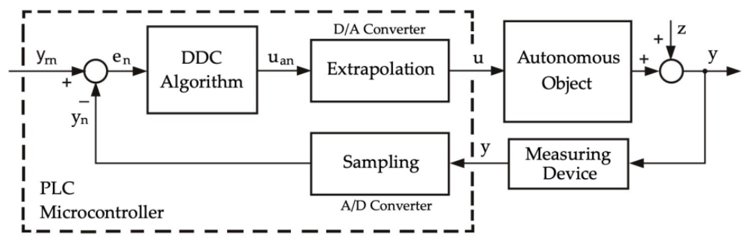
Figure 2.
Examples of autonomous mobile robots: Pallet Jack MiR1200 (Phoenix Mecano) [26] (left); Reach Truck MW-R16 (Multiway) [27] (right).
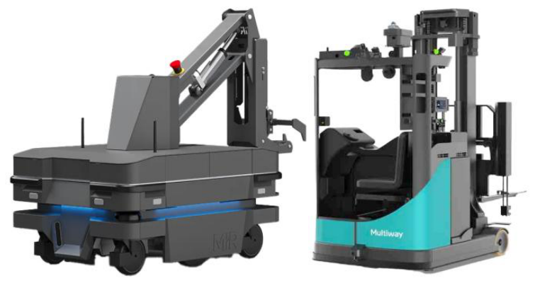
Figure 3.
Computational intelligence algorithms for preventing collisions between an autonomous mobile robot and other mobile robots: x (t)—actual state variables; xm (t)—measured state variables; p (X, Y, t)—optimal and safe robot trajectory.
Figure 3.
Computational intelligence algorithms for preventing collisions between an autonomous mobile robot and other mobile robots: x (t)—actual state variables; xm (t)—measured state variables; p (X, Y, t)—optimal and safe robot trajectory.
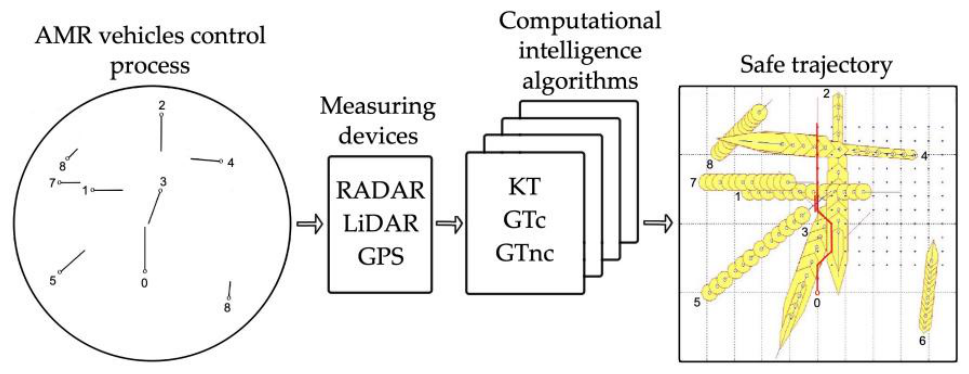
Figure 4.
Determination of the set L0 of the course change to the left and the set R0 of the course change to the right or reducing the speed of robot to 0 to maintain a safe passing distance from robot j at a safe distance Ds.
Figure 4.
Determination of the set L0 of the course change to the left and the set R0 of the course change to the right or reducing the speed of robot to 0 to maintain a safe passing distance from robot j at a safe distance Ds.
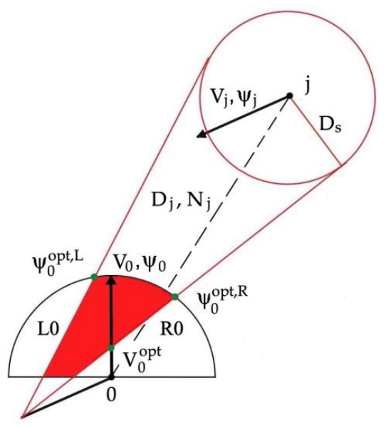
Figure 5.
Illustrating the dangerous area of approach of robots 0 and j in the form of a hexagonal neural domain: d*—final deviation of the safe trajectory of robot 0 from the given direction of movement.
Figure 5.
Illustrating the dangerous area of approach of robots 0 and j in the form of a hexagonal neural domain: d*—final deviation of the safe trajectory of robot 0 from the given direction of movement.
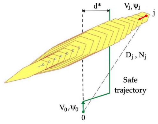
Figure 6.
The maneuvering strategies for robot 0 are expressed as (ψ0, V0), while those for robot j are represented as (ψj, Vj) within the context of the matrix game framework.
Figure 6.
The maneuvering strategies for robot 0 are expressed as (ψ0, V0), while those for robot j are represented as (ψj, Vj) within the context of the matrix game framework.
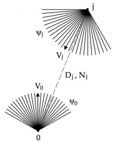
Figure 7.
Safe trajectory of the autonomous mobile robot 0 at safe distance, Ds = 6 m, determined by the GTnc algorithm (left). Comparison of KT, DT, GTc, and GTnc algorithms (right).
Figure 7.
Safe trajectory of the autonomous mobile robot 0 at safe distance, Ds = 6 m, determined by the GTnc algorithm (left). Comparison of KT, DT, GTc, and GTnc algorithms (right).
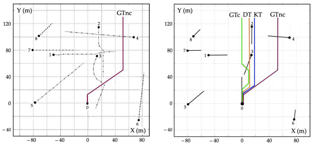
Figure 8.
Examples of autonomous vehicles: JAGUAR I-PACE (Waymo) [28] (left); Reach Truck MW-R16 (Multiway) [29] (right).
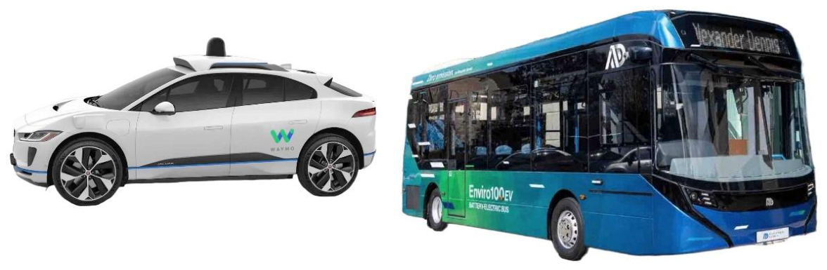
Figure 9.
Hierarchical system for controlling a group of autonomous vehicles.
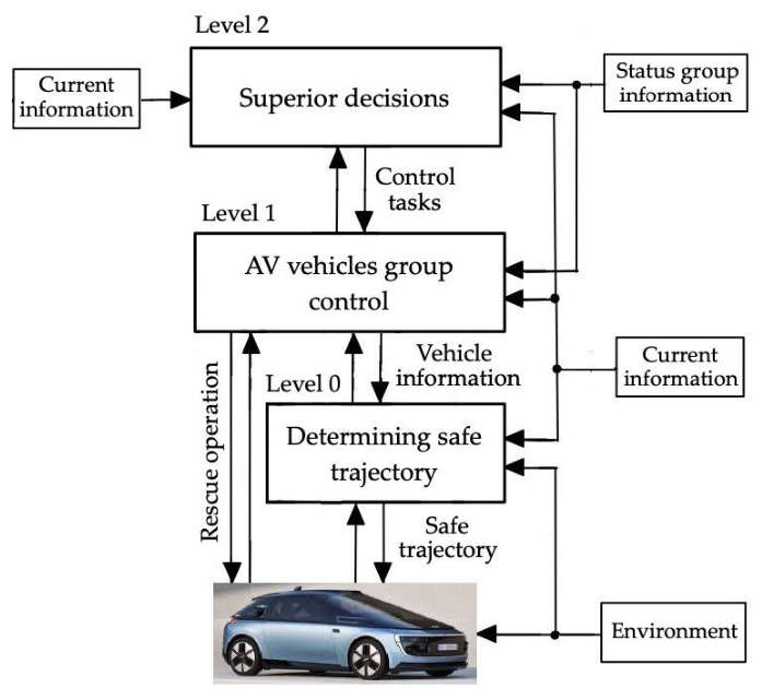
Figure 10.
The road situation of a group of autonomous vehicles: σ0 and χ0 are the speed and heading of the primary autonomous vehicle; σn and χn are the speed and heading of the n-th autonomous vehicle, n = 1, …, N; φn and δn are the bearing and distance to the n-th autonomous vehicle; X0 and Y0 are the coordinates of the primary autonomous vehicle’s position; Xn and Yn are the coordinates of the n-th autonomous vehicle’s position.
Figure 10.
The road situation of a group of autonomous vehicles: σ0 and χ0 are the speed and heading of the primary autonomous vehicle; σn and χn are the speed and heading of the n-th autonomous vehicle, n = 1, …, N; φn and δn are the bearing and distance to the n-th autonomous vehicle; X0 and Y0 are the coordinates of the primary autonomous vehicle’s position; Xn and Yn are the coordinates of the n-th autonomous vehicle’s position.
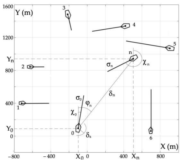
Figure 11.
Graphic interpretation of the areas of permitted maneuvers (green) and prohibited maneuvers (red) for driving while maintaining a safe overtaking distance δs in a group of autonomous vehicles.
Figure 11.
Graphic interpretation of the areas of permitted maneuvers (green) and prohibited maneuvers (red) for driving while maintaining a safe overtaking distance δs in a group of autonomous vehicles.
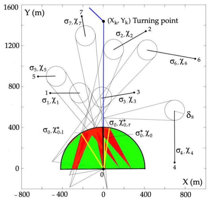
Figure 12.
Comparison of trajectories of autonomous vehicles in multidirectional (left) and one-way traffic (right) determined according to the KT, DT, GTc, and GTnc algorithms with a safe overtaking distance of δs.
Figure 12.
Comparison of trajectories of autonomous vehicles in multidirectional (left) and one-way traffic (right) determined according to the KT, DT, GTc, and GTnc algorithms with a safe overtaking distance of δs.
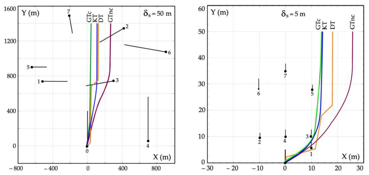
Figure 13.
Values of final deviation of trajectories from their initial values for autonomous vehicles in multidirectional (left) and one-way traffic (right).
Figure 13.
Values of final deviation of trajectories from their initial values for autonomous vehicles in multidirectional (left) and one-way traffic (right).
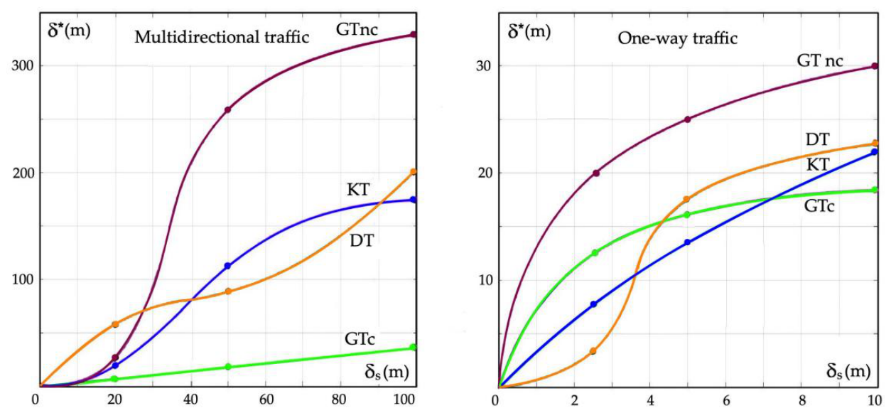
Figure 14.
Examples of autonomous biomimetic land vehicles: Spot and Atlas (Boston Dynamics) (left) [30]; Mole_Bot (Kaist) (right) [31].
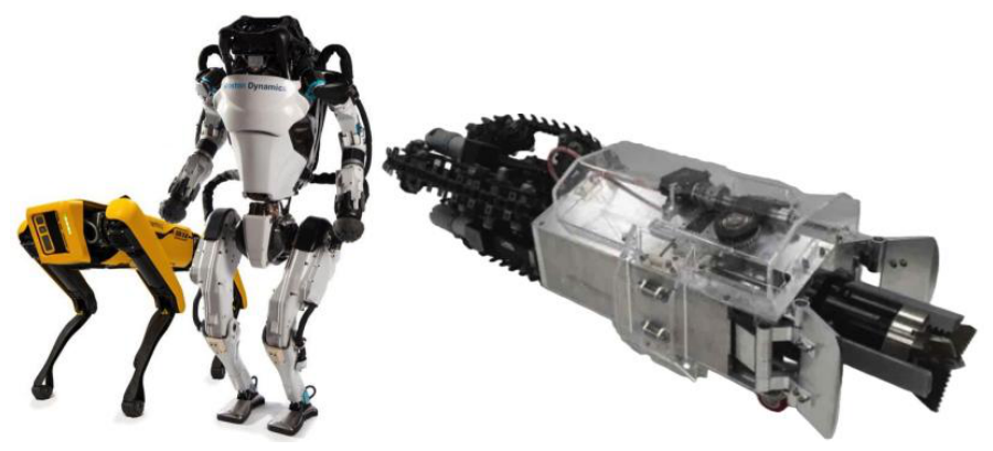
Figure 15.
Examples of autonomous surface vehicles: WAM-F (Ocean Power Technology) [32] (left); Voyager (Salidrone) [33] (right).
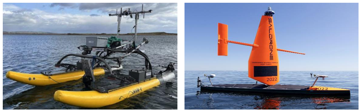
Figure 16.
Block diagram of the control process in a group of autonomous surface vehicles.
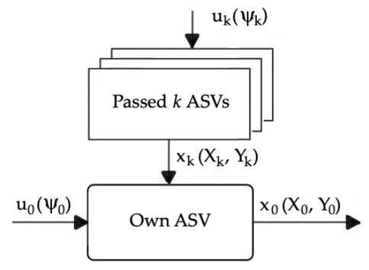
Figure 17.
Visualization of the movement of autonomous surface vehicles: V0 and ψ0 are the speed and heading of the primary vehicle; Vk and ψk are the speed and heading of vehicle k; Dk and Nk are the distance and bearing to vehicle k; and are the minimum distance and time to pass vehicle k; Ds is the safe distance for passing vehicles; (X,Y) are the coordinates of the vehicles’ positions.
Figure 17.
Visualization of the movement of autonomous surface vehicles: V0 and ψ0 are the speed and heading of the primary vehicle; Vk and ψk are the speed and heading of vehicle k; Dk and Nk are the distance and bearing to vehicle k; and are the minimum distance and time to pass vehicle k; Ds is the safe distance for passing vehicles; (X,Y) are the coordinates of the vehicles’ positions.
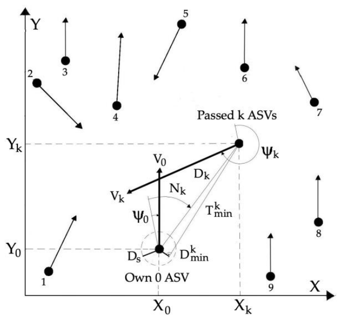
Figure 18.
The set of the number of acceptable strategies i for the primary vehicle 0 and the number of acceptable strategies j for the other vehicles.
Figure 18.
The set of the number of acceptable strategies i for the primary vehicle 0 and the number of acceptable strategies j for the other vehicles.
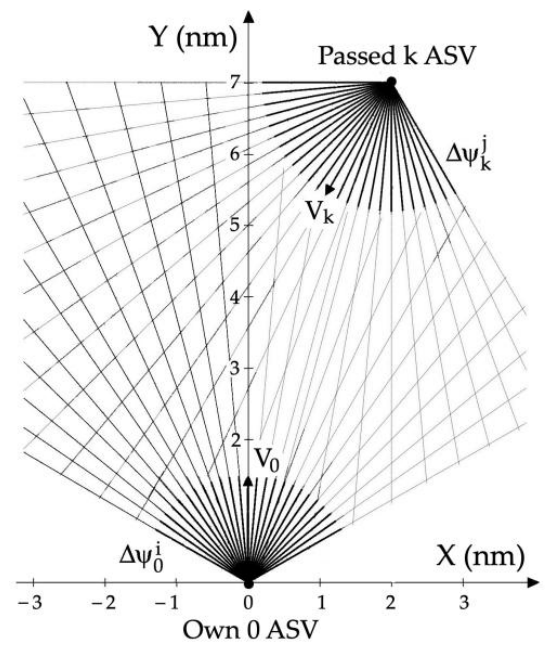
Figure 19.
Safe game GT (left) and non-game KT (right) trajectories of ASV using sets of maneuvering strategies of vehicles i = 13 and j = 25.
Figure 19.
Safe game GT (left) and non-game KT (right) trajectories of ASV using sets of maneuvering strategies of vehicles i = 13 and j = 25.
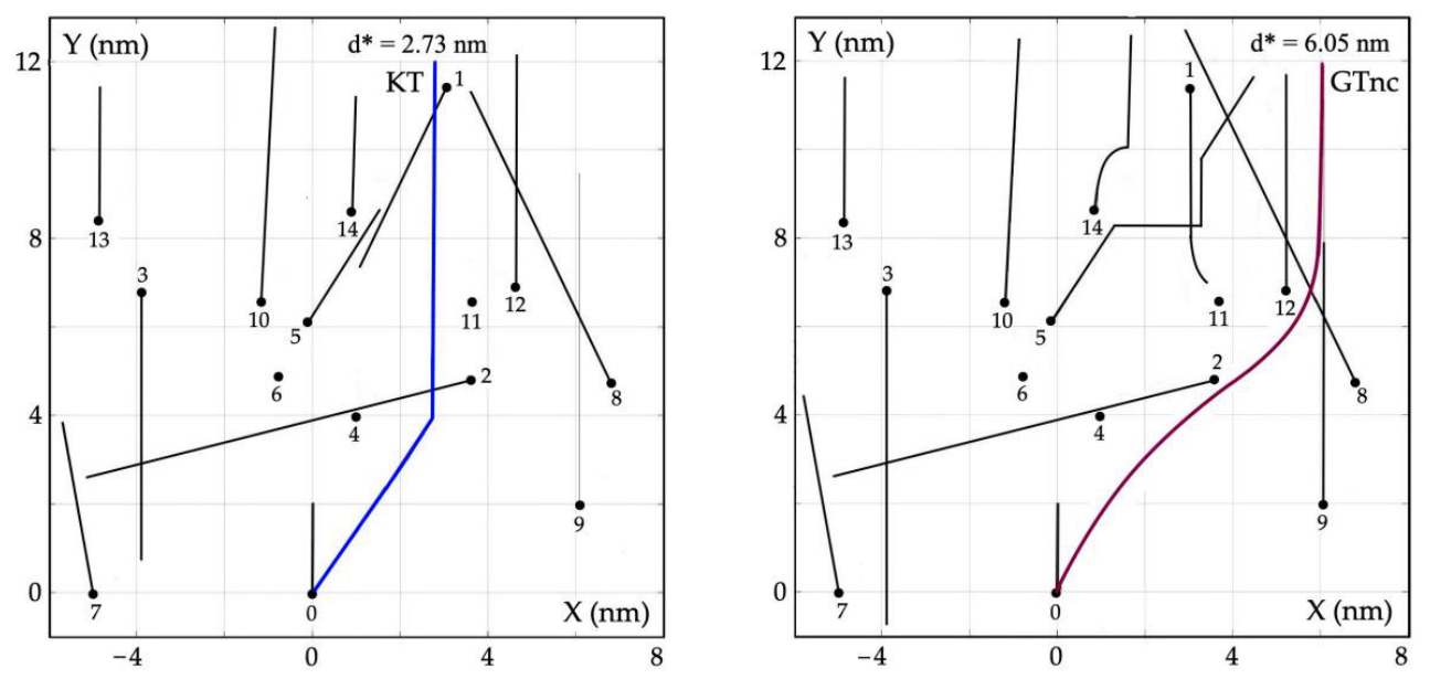
Figure 20.
Examples of autonomous ships—MASS: LNG carrier m/v PRISM COURAGE [34] (left) and ferry m/f FALCO [35] (right).
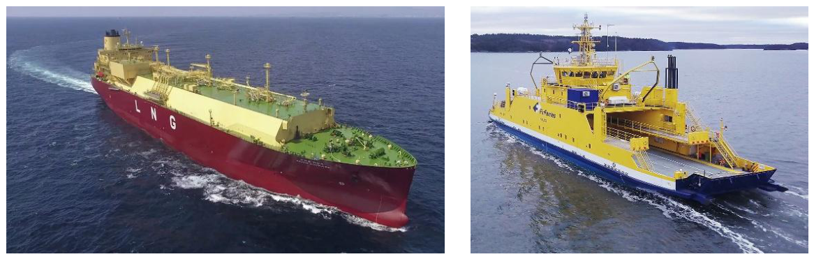
Figure 21.
Multi-layer structure of the MASS group control system.
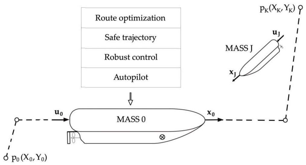
Figure 22.
Determining the optimal route of the MASS using the OR algorithm in the Gulf of Mexico during a hurricane event [36].
Figure 22.
Determining the optimal route of the MASS using the OR algorithm in the Gulf of Mexico during a hurricane event [36].
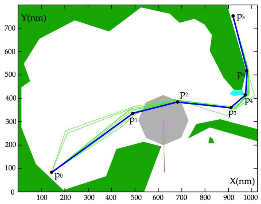
Figure 23.
Illustrating possible trajectories of the MASS.
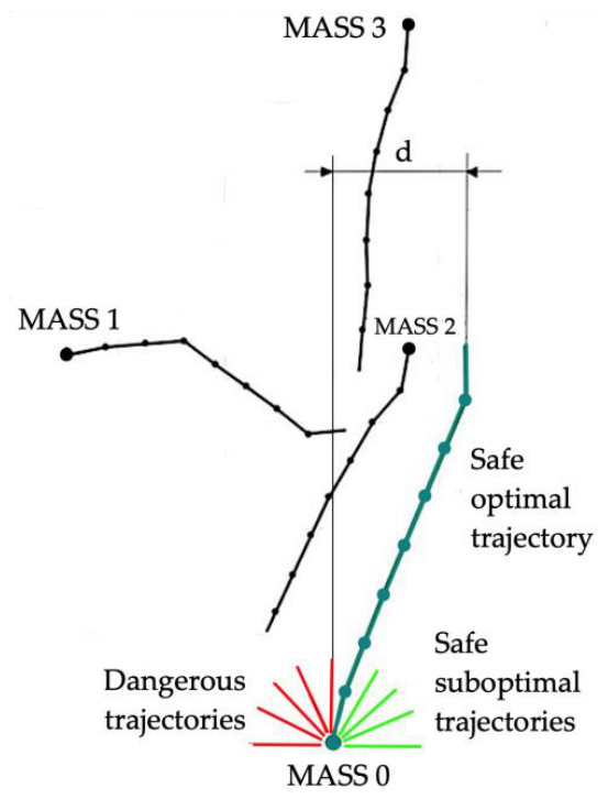
Figure 24.
The quantities describing the movement of MASSs as they pass: ψ0 and V0 are the course and speed of own ship 0; ψjand Vj are the course and speed of ship j; Xj and Yj are the coordinates of ship j.
Figure 24.
The quantities describing the movement of MASSs as they pass: ψ0 and V0 are the course and speed of own ship 0; ψjand Vj are the course and speed of ship j; Xj and Yj are the coordinates of ship j.
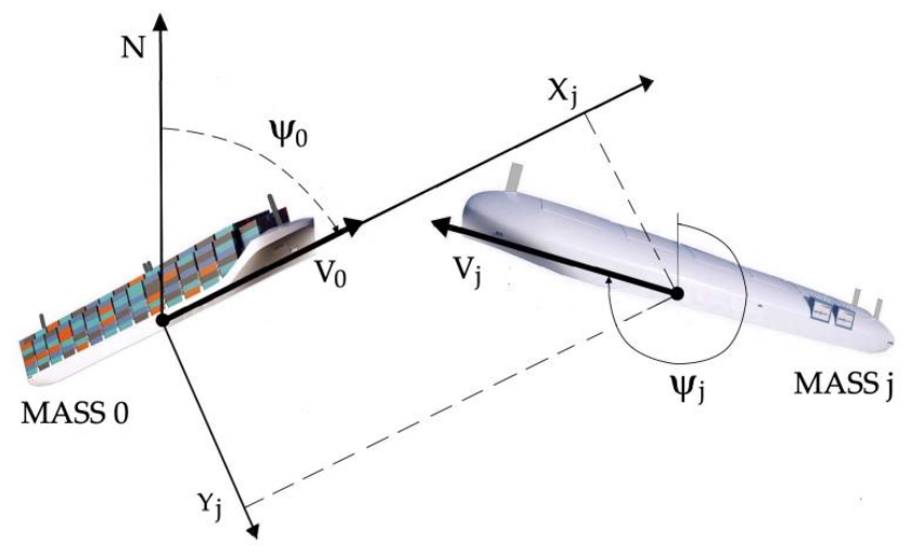
Figure 25.
Geometric determination of the sets of permissible maneuvers of the MASS 0 (green color) in order to pass the MASS j at a safe distance Ds.
Figure 25.
Geometric determination of the sets of permissible maneuvers of the MASS 0 (green color) in order to pass the MASS j at a safe distance Ds.
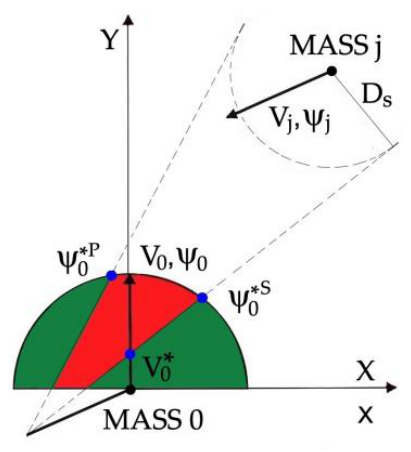
Figure 26.
Dynamic programming grid of the optimal dynamic trajectory of the MASS 0, where t* is the optimal, minimum time of ship movement; d is the deviation of the optimal trajectory from the initial direction of movement; Δx is the density of the dynamic programming grid; and n is the number of the calculation stage.
Figure 26.
Dynamic programming grid of the optimal dynamic trajectory of the MASS 0, where t* is the optimal, minimum time of ship movement; d is the deviation of the optimal trajectory from the initial direction of movement; Δx is the density of the dynamic programming grid; and n is the number of the calculation stage.
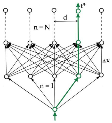
Figure 27.
An artificial neural network that adjusts the size of the possible collision area depending on the collision risk value.
Figure 27.
An artificial neural network that adjusts the size of the possible collision area depending on the collision risk value.
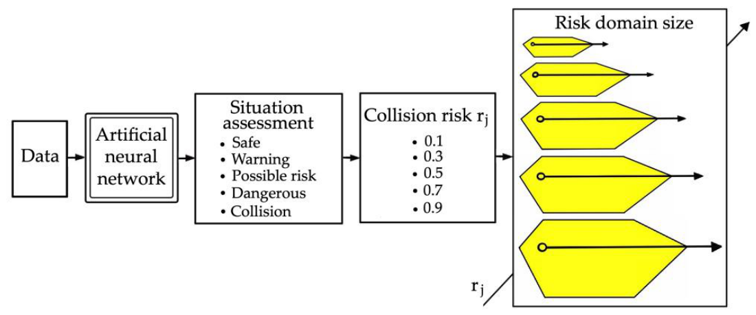
Figure 28.
Comparison of safe trajectories of MASS 0.
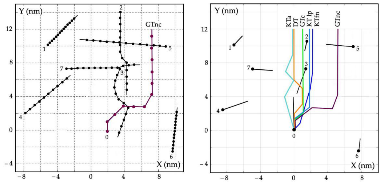
Figure 29.
Examples of autonomous underwater vehicles: Ghost Shark XL (Anduril Industries) [37] (left); Hugin (Konsberg) [38] (right).
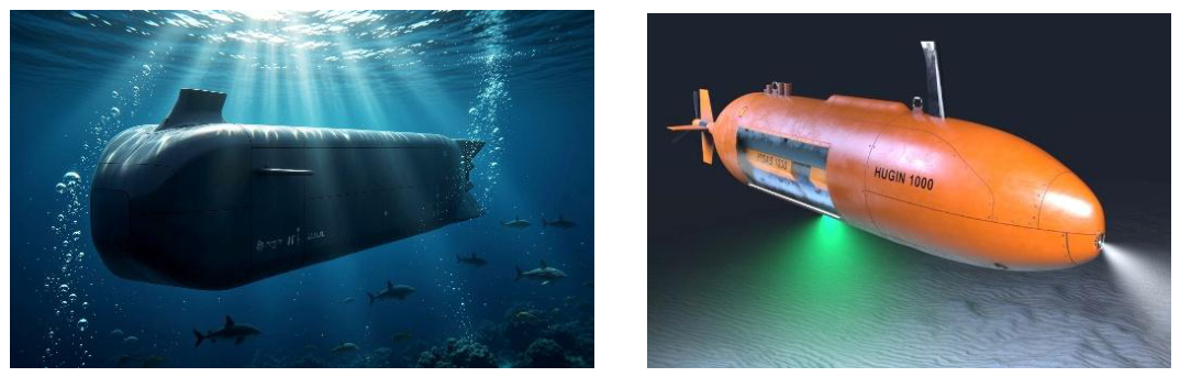
Figure 30.
The process of searching the port area in Gdynia using a multi-agent system [39].
Figure 30.
The process of searching the port area in Gdynia using a multi-agent system [39].
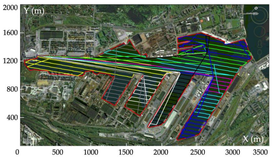
Figure 31.
The set route of an autonomous underwater vehicle.
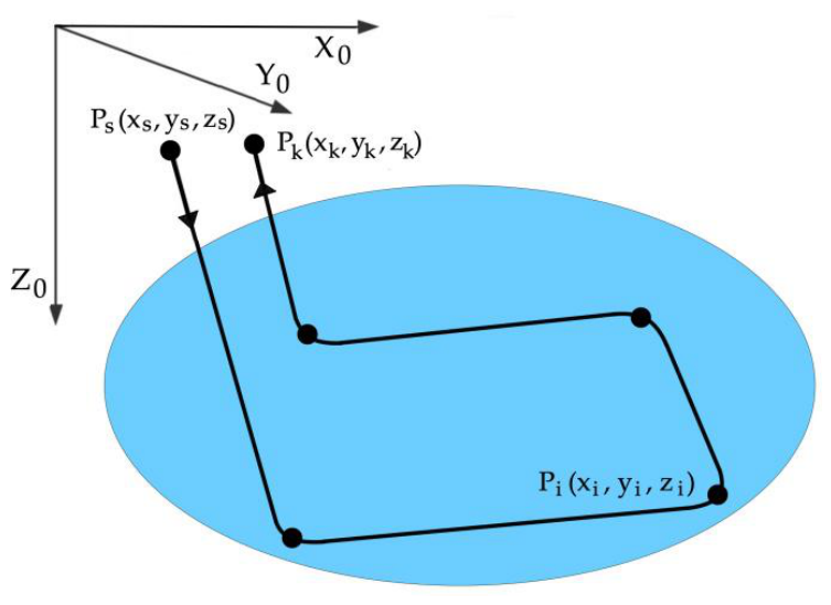
Figure 32.
Trajectory stabilization system of an AUV vehicle: Pi (xi, yi, zi) are the reference positions of the subsequent trajectory sections, P (x, y, z) is the actual position of the vehicle, ψr is the reference course, and zr is the reference draft of the vessel.
Figure 32.
Trajectory stabilization system of an AUV vehicle: Pi (xi, yi, zi) are the reference positions of the subsequent trajectory sections, P (x, y, z) is the actual position of the vehicle, ψr is the reference course, and zr is the reference draft of the vessel.
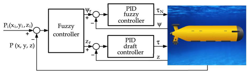
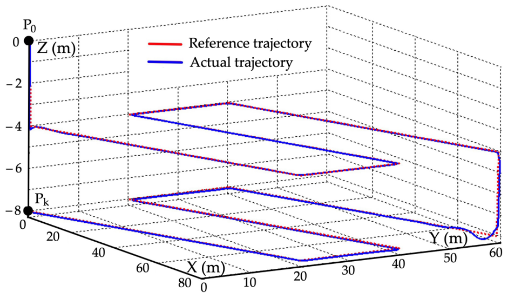
Figure 34.
Examples of autonomous biomimetic water vehicles: BioSwimmer (Boston Engineering) (left) [40]; RoboLobster (Lobster Robotics) (right) [41].
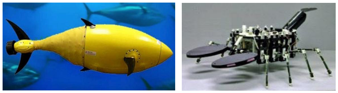
Figure 35.
Examples of autonomous aerial vehicles: Draganfly Heavy Lift Drone (Draganfly) [42] (left) and Mugin-5 Pro (Muginuav) [43] (right).
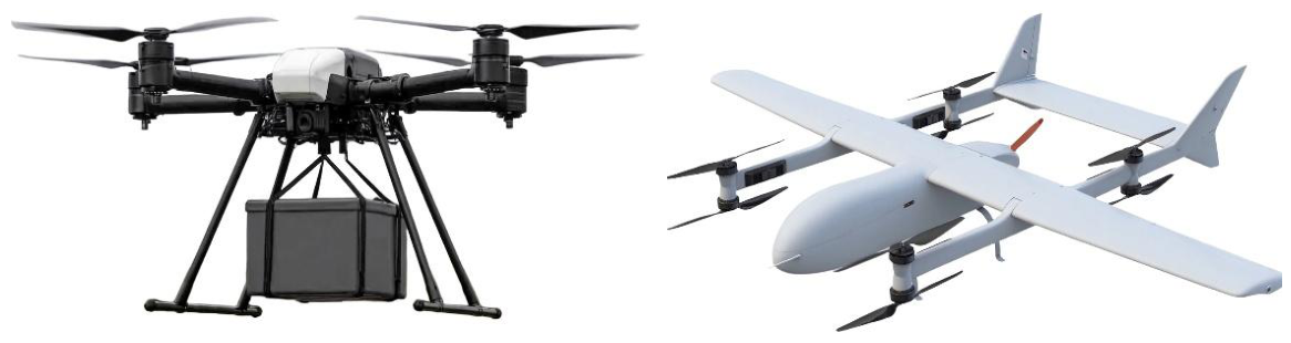
Figure 36.
Passing by the primary AAV 0 with speed v and heading ψ and encountering an AAV k moving with speed vk and heading ψk.
Figure 36.
Passing by the primary AAV 0 with speed v and heading ψ and encountering an AAV k moving with speed vk and heading ψk.
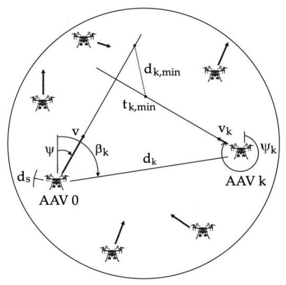
Figure 37.
State variables of autonomous aerial vehicles: s0 (ψ0, v0) are strategies of the primary vehicle; sk (ψk, vk) are strategies of the k vehicle; rk (s0, sk) represents the risk of collision of the primary vehicle with the k encountered vehicle.
Figure 37.
State variables of autonomous aerial vehicles: s0 (ψ0, v0) are strategies of the primary vehicle; sk (ψk, vk) are strategies of the k vehicle; rk (s0, sk) represents the risk of collision of the primary vehicle with the k encountered vehicle.
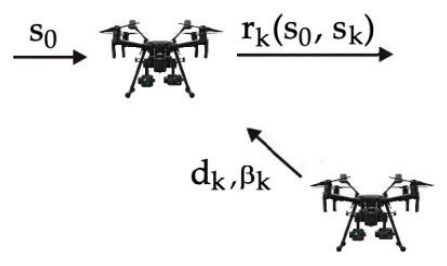
Figure 38.
Collision risk value depending on the smallest values of distance and approach time of aerial vehicles: (a) light traffic; (b) medium traffic; (c) heavy traffic.
Figure 38.
Collision risk value depending on the smallest values of distance and approach time of aerial vehicles: (a) light traffic; (b) medium traffic; (c) heavy traffic.
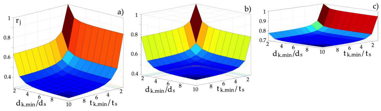
Figure 39.
Comparison of safe trajectories of AAV 0 when passing K = 3 encountered autonomous aerial vehicles: determined by the GTnc algorithm in heavy traffic when ds = 12 m (left), comparison of the KT, GTc, and GTnc algorithms in light traffic when ds = 4 m and in heavy traffic when ds = 12 m (right).
Figure 39.
Comparison of safe trajectories of AAV 0 when passing K = 3 encountered autonomous aerial vehicles: determined by the GTnc algorithm in heavy traffic when ds = 12 m (left), comparison of the KT, GTc, and GTnc algorithms in light traffic when ds = 4 m and in heavy traffic when ds = 12 m (right).
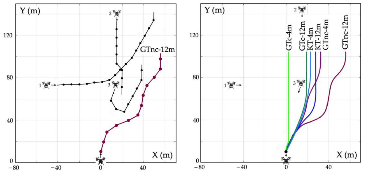
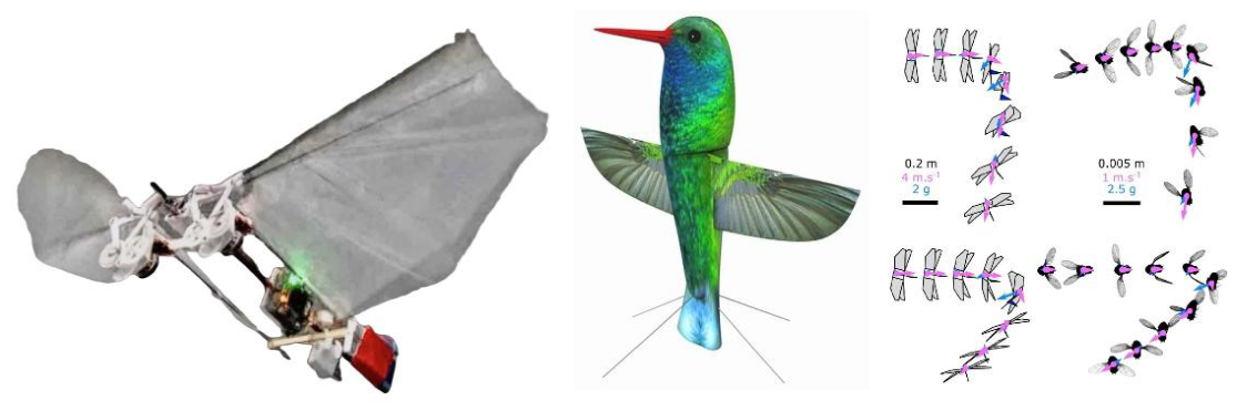
Disclaimer/Publisher’s Note: The statements, opinions and data contained in all publications are solely those of the individual author(s) and contributor(s) and not of MDPI and/or the editor(s). MDPI and/or the editor(s) disclaim responsibility for any injury to people or property resulting from any ideas, methods, instructions or products referred to in the content. |
© 2026 by the authors. Licensee MDPI, Basel, Switzerland. This article is an open access article distributed under the terms and conditions of the Creative Commons Attribution (CC BY) license (http://creativecommons.org/licenses/by/4.0/).
Copyright: This open access article is published under a Creative Commons CC BY 4.0 license, which permit the free download, distribution, and reuse, provided that the author and preprint are cited in any reuse.