

Submitted:
08 July 2026
Posted:
09 July 2026
You are already at the latest version
Abstract
Effective decision-making in reservoir management requires accurate insight into interwell fluid-flow communication and the dynamic response of fluids in fractured reservoirs. This study builds upon prior Visibility Graph (VG) analysis and Multiplex Network (MN) methodologies to infer potential interwell communication patterns associated with subsurface fluid flow connectivity. We leverage VG-derived adjacency matrices in conjunction with production and injection time series, treating them as dynamic reservoir responses and transforming them into image representations using the Gramian Angular Field (GAF) method. These GAF images then serve as input to a Convolutional Neural Network (CNN) for classifying zones associated with different levels of inferred interwell fluid-flow connectivity. The result is a dual-path framework that combines structural insights from VG with learned spatiotemporal patterns from production-injection dynamics, enabling the generation of spatial diagnostic maps for reservoir planning. These maps provide a proxy interpretation of possible preferential communication pathways associated with production-injection response. The proposed method supports practical decision-making by providing interpretable spatial representations of reservoir connectivity and production-injection interaction patterns. Comparison of the resulting metrics demonstrates the potential of the method to support reservoir diagnostics and identify zones where connectivity-related behavior may require further engineering evaluation. Furthermore, we assess two GAF-based input strategies, the impact of data augmentation, and the resulting spatial classification of interwell connectivity zones.
Keywords:
interwell fluid-flow connectivity
; fractured reservoirs
; production-injection dynamics
; subsurface flow
; Gramian Angular Field
; convolutional neural networks
; porous media
1. Introduction
Reservoir management involves complex decision-making under uncertainty, particularly when optimizing production and interpreting interwell fluid-flow connectivity from production and injection responses [13,14,15]. Most assessment techniques rely heavily on geological and geophysical data, which may be incomplete or insufficient to fully characterize dynamic reservoir behavior. However, available information often provides only limited insight into in in situ properties, and may not be updated frequently enough to represent the evolving petrophysical and flow conditions of the reservoir. In addition, conventional numerical simulations and heuristic methods remain essential for reservoir analysis, but they can be computationally intensive and difficult to interpret when rapid diagnostic assesment is required [12]. Recent advances in visibility graph (VG) and multiplex network analysis provide a data-driven framework for inferring interwell connectivity and fluid-flow interaction patterns from production and injection signals [18]. These techniques use metrics such as average edge overlap and interlayer mutual information to characterize persistent connectivity structures and temporal variations in interwell communication. However, translating these inferred connectivity patterns into spatially interpretable reservoir zones remains a significant challenge.
Accurate identification of interwell communication pathways is critical for understanding fluid displacement and optimizing development strategies in fractured reservoirs. In fractured systems, these pathways may reflect preferential flow channels that influence injection efficiency, sweep behavior, and production response. Effective modeling of such interwell communication informs decisions regarding well placement, stimulation, and reservoir management. Traditional approaches, such as pressure transient analysis [7], and tracer tests [5,6], can require high-cost instrumentation, extensive prior knowledge, or specific operational conditions, and may not always capture dynamic production behavior in heterogeneous systems [8,9,11].
Recent advances in Machine Learning (ML) and Deep Learning (DL) offer data-driven approaches for modeling reservoir connectivity from production, injection, and spatial response data [4]. Techniques such as Long-Short-Term Memory (LSTM) networks, Recurrent Neural Networks (RNNs), and Graph Neural Networks (GNNs) have shown potential for time series prediction and spatial inference in networked geoscience and subsurface systems [20,22,24]. However, many of these models require long temporal histories or rely on spatial regularization that may be too coarse to capture localized interwell communication in fractured domains.
To address this limitation, we propose a dual-path convolutional framework that uses Gramian Angular Field (GAF) representations [25] to encode production and injection dynamics, as well as interwell interaction matrices, into 2D image representations suitable for CNN-based analysis [16]. These representations serve as inputs to a Convolutional Neural Network (CNN) [19] for connectivity-zone classification and segmentation, combining temporal signal analysis with the spatial interpretation of interwell communication patterns [3]. The proposed dual-path framework includes two complementary processing pipelines designed to evaluate whether different GAF-based representations provide consistent spatial interpretations of reservoir connectivity:
- Type A: Converts sliding windows of well-specific production/injection time series into GAF images to represent local well-level dynamic responses.
- Type B: Encodes full interaction matrices based on flow ratio dynamics into GAF images at each time step to represent system-level interwell interaction patterns.
The characteristics of these pipelines are schematically illustrated in Figure 1.
This dual approach captures both localized well-level dynamic behavior and system-wide interaction structure, improving robustness resulting in improved robustness, interpretability, and spatial coverage. We further integrate interconnectivity scores and well coordinates into the CNN pipeline to incorporate structural and spatial reservoir context. Accordingly, our study evaluates the comparative effectiveness of each GAF type, the impact of data augmentation, and the resulting spatial classifications of reservoir connectivity zones. The main contribution of this work is the integration of GAF-based dynamic response encoding with CNN-based spatial classification to support the identification of reservoir zones associated with different levels of interwell fluid-flow communication. By transforming production and injection time series into structured representations, this framework supports the inference of high-probability interwell communication zones with minimal a priori assumptions.
2. Methodology
The proposed complementary framework combines temporal patterns extracted from production and injection flow-rate time series with a static interwell interconnectivity matrix [18]. This approach enables the segmentation and classification of reservoir regions associated with different levels of inferred interwell fluid-flow connectivity by applying a CNN architecture to GAF-encoded dynamic data [16]. The procedure converts production and injection time series into 2D GAF representations that encode dynamic reservoir-response patterns. The encoded temporal and interaction patterns are then extracted using CNN architectures.
Thus, the complementary dual-path architecture consists of GAF transformations applied to two different preprocessed data representations, labeled as Type A and Type B.
The key steps involved in this redundant architecture are:
Data acquisition and preprocessing. The framework requires a static interwell interconnectivity matrix, production and injection flow-rate time series for the study period, and the projected spatial coordinates of the wells. In the Type A pathway, historical production or injection flow rates from individual wells are segmented using a sliding window technique prior to their GAF transformation. This approach emphasizes temporal signal patterns within individual wells. In the Type B pathway, the flow rates of all wells at each timestamp are mapped into a matrix representation, referred to as a state matrix. This approach emphasizes system-level interwell interaction patterns and the temporal evolution of reservoir flow states. In this sense, Type A is intended to represent local dynamic well response, whereas Type B is intended to represent field-scale interaction states related to interwell fluid communication.
As a next step, the time series was normalized using min-max scaling and then rescaled to the interval for angular encoding:
Time series to image transformation. The time series were transformed into image-like representations using the GASF method. This transformation encodes time-dependent production and injection response patterns into 30×30 grayscale images that retain temporal relationships.
For a given normalized time series , we define the polar encoding
The GAF matrix is then constructed with elements given by:
Equation 3 refers to the Gramian Angular Summation Field (GASF), which captures temporal correlations by encoding pairwise angular relationships between time points. The resulting matrix is symmetric and emphasizes consistent signal co-movement patterns. By construction, this representation emphasizes global similarity between time points.
Although GASF is traditionally used to encode global correlations in sequential data, its application to Type B allows the model to capture structured interwell relationships within each time-step interaction matrix. This structured encoding supports CNN-based detection of latent interwell interaction patterns in reservoir dynamics.
Table 1 shows the comparison between the GASF transformations applied to Type A and Type B images.
Data augmentation.
The effects of data scarcity are reduced by applying statistical augmentation techniques to the dataset. Gaussian noise, Fourier perturbations, and time series warping are introduced to generate the augmented dataset. These procedures are intended to improve the robustness of the model by introducing variability into the original data while preserving its structural characteristics, a desirable feature for model generalization.
Gaussian Noise Injection. Gaussian Noise injection was used to simulate realistic sensor or measurement variability. Let be a normalized time series. We generate an augmented series by adding zero-mean Gaussian noise:
where controls the noise level. In practice, small values of (e.g., 0.01, to 0.05) are used to avoid excessive alteration of the overall distribution.
Fourier Transform Perturbation. Fourier transform perturbation modifies frequency components while preserving the main temporal structure, thereby simulating plausible phase or trend distortions.
The Discrete Fourier Transform (DFT) is applied to the original signal: . We then apply a perturbation to the phase components of the frequency domain.
where is the original phase and is a small uniform random phase shift. The inverse DFT gives the augmented time series:
This preserves the spectral magnitude while introducing plausible temporal deformations.
Time Series Warping (Time-Axis Warp).
Time Series warping introduces nonlinear distortions to simulate real-world variability in rate or shape. A smooth, monotonic warping function is applied to the time axis:
where is drawn from a low-frequency noise process (e.g., cubic spline over random anchor points), and controls smoothness. Interpolation is used to sample the values at warped indices.
Using the above techniques to address data imbalance, synthetic images were generated for underrepresented classes, notably Class 2. This balancing procedure was later evaluated using the classification performance metrics reported in the Results section. The data augmentation was constrained to preserve the overall structure of production and injection responses, so that synthetic samples remained consistent with plausible reservoir-rate variability.
Label construction. To support the regression and classification objectives, four label sets were derived from the interconnectivity matrix: Total, Injection, Ratio, and Class. The Total label is defined as the sum of all absolute interconnections per well. The Injection label is defined as the sum of absolute interconnections associated with injection wells. The Ratio label is defined as the ratio between injection-related interconnectivity and total interconnectivity per well.
Finally, the Class label is derived from Ratio thresholds and divided into Low, Medium, High interconnectivity categories. This label is used to map the spatial distribution of inferred connectivity regions using the well coordinates. These categories are interpreted as weak, intermediate, and strong inferred interwell communication, respectively, and are used as proxy indicators of spatial variability in reservoir connectivity
Convolutional Neural Network. Once the data are transformed into image-like representations, the classification tasks are handled by a CNN architecture designed to extract hierarchical features associated with dynamic reservoir responses and interwell interaction patterns. The CNN architecture used in this work follows the standard feedforward CNN pipeline (see Figure 2):
- 1.
- Convolution + ReLU: Feature extraction through convolution filters followed by the ReLU activation function .
- 2.
- Pooling: Dimensionality reduction via max pooling or average pooling.
- 3.
- Flattening: Conversion of feature maps into 1D vectors.
- 4.
- Fully connected layers: Transformation of features into a final classification vector.
- 5.
- Softmax: Normalized output over the class space
As shown in Table 1, Type A GASF images represent individual well behavior, while Type B GASF images represent system-level interwell dynamics. The Type A experiments focused on classifying zone probabilities using time-series data transformed into GASF images and combined with static interconnectivity features. These GASF images encode production or injection behavior over time for individual wells, while the interconnectivity matrix provides inferred structural relationships between wells.
Model architecture and training. The resulting image representations are fed into a CNN to learn patterns associated with subsurface flow dynamics and to classify reservoir regions according to the established labels.
Spatial visualization and analysis. To interprate model predictions in a geographical context, different visualizations are proposed, included zone probability heatmaps and well-label zone classification maps.
Figure 1 summarizes the two complementary pipelines, Type A and Type B. It shows the process from time-series normalization and GAF transformation to CNN-based reservoir connectivity classification.
3. Results
The proposed framework was applied to a fractured reservoir case study involving production and injection data from 12 production wells and 4 injection wells.
3.1. Data Acquisition and Preprocessing
The study incorporated three primary sources of field data: a static 16×16 interconnectivity matrix, interconnectivity matrix inferred for 12 production wells and 4 , production and injection flow-rate time series for the study period, and spatial well coordinates used as additional model features. It is important to highlight that for these wells, the geographical coordinates are given as longitude and latitude respectively and were used as features encoded together with the time series datapoints. The wells to were identified as production wells and to as injection wells. This configuration provides a representative setting for evaluating how production and injection signals reflect possible interwell communication in a fractured reservoir.
To prepare the dataset for modeling, missing values in the time series were interpolated and the min-max scaling normalization technique was applied to ensure scale consistency.
After these pre-processing steps were applied to the production and injection flow-rate data, the resulting dataset was prepared for the GASF transformation.
3.2. GASF Images Generation
To predict interwell connectivity zones, the dual-path modeling framework applied GASF transformations to two types of reservoir input data: production/injection flow-rate time series per well (Type A) and interwell state matrices (Type B). In both pathways, GASF was used to encode either temporal well-level responses (Type A) or snapshot interwell interaction matrices (Type B).
This transformation encodes the temporal evolution of the production and injection responses into a structured image G, making local and global temporal correlations accessible to CNN spatial filters.
Figure 1 illustrates this two-branch GASF modeling pipeline. In the Type A pathway, the historical production or injection time series of each well were segmented using a sliding window technique, transformed into GASF images, and classified using CNNs architectures. This approach emphasizes temporal signal patterns within individual wells.
In contrast, the Type B pathway processes the matrix of production/injection ratios between wells at each time step, encoding the system-level interwell interaction structure as a 2D image. These snapshots were also converted into GASFs and used for training with CNN models.
By combining these complementary perspectives, the model captures both temporal well behavior and system-level interwell correlations, enhancing the robustness of zone classification.
This methodology integrates dynamic flow-response features and spatial interwell information for connectivity-zone classification and interwell fluid-flow analysis in fractured reservoir systems.
3.3. Data Augmentation
Augmentation techniques, such as Gaussian noise, Fourier transform perturbations, and time-series warping, were applied two both input pathways.
Gaussian noise was applied with controlling the noise level. This level introduces realistic noise without distorting the time series dynamics. In the case of Fourier Transform Perturbation the value used was . This phase shift modifies the periodicity slightly, simulating distortions in flow patterns while preserving signal energy. For time-series warping, four anchor points were used, with a warp magnitude of and cubic spline interpolation. These parameters introduce smooth nonlinear distortions in local signal speed without abrupt jumps.
Type A – Sliding time series GASF
A total of 1,154 GASF images were generated using sliding-window transformations of per-well production and injection logs, including the augmentation techniques described above.
Type B – Flow Interaction Matrix GASF
A second set of 112 GASF images (Type B) was derived by converting flow interaction matrices—representing all well interactions at each time step into GASF representations. Augmentation using Fourier and noise-based perturbations expanded this set to 1,000 samples.
3.4. Model Architecture and Training
After the data pre-processing stage, data augmentation, label determination, and data balance engineering, we trained a set of CNN-based architectures enhanced with spatial and structural input vectors.
The model inputs include:
- GASF images (30××30×1): GASF-encoded representations of production/injection dynamics for Type A and Type B.
- Flattened interconnectivity matrix (256D): Encodes the static inferred connectivity relationships among the 16 wells for the study period.
- Well coordinate vector (32D): Comprises normalized X and Y coordinates for each of the 16 wells.
The CNN path processes the GASF images using two convolutional layers followed by max pooling and flattening. Then, this representation is concatenated with the flattened interconnectivity vector and coordinate vector. The merged feature set is passed through two dense layers with dropout regularization, concluding with an output layer for either regression (total connectivity, injection connectivity, ratio) or classification (zone label).
This combined input strategy allows the model to leverage temporal production/injection dynamics from the GASF images, spatial location from the coordinate vector, and structural relationships from the interconnectivity matrix. The model is trained using a standard 80/20 split, and performance is evaluated with RMSE for regression outputs and accuracy for classification.
The architecture also provides a flexible basis for future extensions, such as attention mechanisms to emphasize influential interwell regions.
3.5. Quantitative Results for Experiments Type A and Type B
This section presents the evaluation metrics, spatial visualizations, and interpretative analysis of the proposed GASF-CNN framework for reservoir connectivity-zone classification. The results are analyzed in terms of prediction accuracy, spatial consistency, and potential implications for reservoir management. For Type A, four models were trained to predict zone-related labels derived from the interconnectivity matrix:
- Label Total (regression): RMSE = 1.3914
- Label Injection (regression): RMSE = 0.5704
- Label Ratio (regression): RMSE = 0.2039
- Label Class (classification): Accuracy =
Among these models, the injection-related score achieved the lowest RMSE, suggesting that injection-related connectivity may be more consistently represented in the input features. The Ratio label model also showed a relatively low RMSE, indicating a meaningful relationship between injection dominance and overall interwell connectivity.
The Type A classification accuracy of across three classes (low, medium, high) indicates that individual well-level GASF representations capture some connectivity-related information, but remain insufficient for robust spatial classification. This performance may be influenced by class imbalance, overlapping zone characteristics, or noise introduced during label replication.
For Type B, each GASF image reflects an instantaneous interaction snapshot across all wells. These representations provided more informative system-level interwell features for zone classification and outperformed Type A in classification accuracy.
- CNN Model (Type B): RMSE = 0.2871
- Redundant CNN + Interconnectivity vector: RMSE = 0.2895
- Before class balancing, the weighted classifier accuracy reached , but recall remained low for minority classes.
This behavior suggests that connectivity-zone prediction benefits from representing the reservoir as an interacting flow system rather than as independent well-level time series alone.
The classifier performed well for the dominant class (low probability zones), but showed limited ability to capture medium- and high-probability zones due to severe class imbalance.
3.6. Spatial Visualization of the Results Type A and Type B
To interpret model predictions in a geographic context, multiple spatial visualizations were generated:
- Zone probability heatmap: Interpolated predicted probabilities revealed coherent clusters of medium and high interconnectivity in the northern and central areas of the reservoir, consistent with denser production-injection well arrangements.
- Well labels and zone classification: Each well was labeled with its predicted zone class and surrounded by a 100-meter influence circle to emphasize its local connectivity influence.
These visual outputs support the spatial interpretation of model predictions and provide diagnostic maps for assessing potential interwell communication zones.
For Type A, spatial visualizations were generated to locate probable zones of inferred interwell connectivity. Two representative figures are included:
Zone Probability Heatmap: Displays predicted zone scores over well coordinates, interpolated to show intensity of probable interconnection zones.
Interconnectivity Overlay: Shows inferred connectivity scores overlaid with zone probability predictions and labeled well positions. Circular zone thresholds aid in visually distinguishing low, medium, and high probability regions.
These spatial tools helped translate numerical predictions into operationally meaningful geospatial diagnostics.
To interpret the model predictions in spatial terms:
- Geographical scatter plots of the wells were generated using their coordinates (longitude-latitude).
- Interconnectivity lines (based on matrix thresholds) were overlaid.
- Zone probability heatmaps were created by interpolating predicted probabilities in the geographical space.
Figure 3 was generated to visually support the results and facilitate spatial interpretation. It presents an interpolated heatmap over the geographical area of the reservoir. Warmer zones (red, orange) indicate higher predicted zone probability scores, suggesting stronger inferred interwell connectivity or more pronounced injection-production interaction. Cooler zones represent wells with lower connectivity probabilities. The Well locations are overlaid, color-coded by prediction strength, and labeled for reference.
- The Type B results indicate that well-to-well interactions encoded as temporal flow matrices provide a richer feature space for zone probability estimation.
- The static interconnectivity matrix, when added as a flattened vector, improved regression accuracy, although it did not enable the model to distinguish minority classes in classification.
- Before augmentation, class imbalance remained the most critical challenge. Although class weighting improved some metrics, it was insufficient to enable generalization.
To address data imbalance, synthetic images were generated for underrepresented classes (notably, high interconnectivity Class 2). To evaluate the performance of the classification model after augmenting the underrepresented Class 2 samples, we retrained the Type B CNN classifier. The post-augmentation classification metrics demonstrated a notable improvement in the overall accuracy and class balance:

Table 2.
Classification Report for Three Classes
| Precision | Recall | F1-Score | Support | |
|---|---|---|---|---|
| Class 0 | 0.91 | 1.00 | 0.95 | 67 |
| Class 1 | 1.00 | 0.65 | 0.79 | 66 |
| Class 2 | 0.81 | 1.00 | 0.89 | 67 |
| Accuracy | 0.89 | 200 | ||
| Macro Avg | 0.90 | 0.88 | 0.88 | |
| Weighted Avg | 0.90 | 0.89 | 0.88 |
These results show strong precision and recall for all three classes, especially for Class 2, which was previously underrepresented. The improved balance suggests that the augmentation pipeline enriched the diversity of Class 2 samples and improved their representation during training.
The classification results are further supported by the confusion matrix in Figure 4, where most samples in all three classes are correctly predicted, particularly Classes 0 and Class 2. Class 1, which previously suffered from confusion due to its intermediary nature, also shows strong improvements following the augmentation step.
The Figure 5 illustrates the effectiveness of the balancing process, showing that the model had equal exposure to each interaction zone during training. This correction was crucial in improving the robustness of the model and mitigating classification skew. With a final accuracy of , the classifier shows improved performance for spatial zone estimation based on production-injection interactions.
To explore the spatial implications of the model predictions, we generated two visualizations using the predicted zone labels, well coordinates, and the interconnectivity context.
The visualizations in Figure 6 and Figure 7 show the spatial distribution of predicted zone classes across thw well field smoothed using Kernel Density Estimation (KDE) [17]. KDE estimates a continuous spatial density surface by placing a smoothing kernel over each data point and summing the contributions across the field. Higher-density zones with stronger connectivity predictions (Class 2) tend to cluster around specific wells, particularly in the northeastern and central portions of the field. Figure 8 shows the probability contour distribution of the zone scores obtained for Type B. From a reservoir-flow perspective, these Class 2 clusters can be interpreted as candidate regions of stronger inferred communication, where production response may be more strongly influenced by injection-driven interactions.
4. Discussion
In Figure 6, the Type A model shows more localized inferred connectivity zones around high-production wells, driven mainly by their individual temporal flow behavior. However, it shows limited spatial coherence and is less effective at capturing regional connectivity trends.
In contrast, the Type B model (Figure 7), reflects smoother, spatially consistent patterns across wells, particularly highlighting regional clusters where interwell dynamics are likely to indicate fluid-flow communication. This spatial clustering is consistent with the interwell relationships inferred from the VG-derived interconnectivity matrix and with the expected influence of production-injection interactions in fractured reservoirs. In fractured reservoirs, such spatially coherent zones may indicate preferential communication pathways that influence displacement efficiency, channeling tendency, or sweep heterogeneity.
The results suggest that Type B GAFs provide richer system-level context, yielding stronger classification balance and more coherent representation of field-scale connectivity behavior in the present case study. These zones help visualize localized regions of stronger inferred interwell communication, which may support the prioritization of monitoring , reservoir management, or intervention strategies.
This comparison supports the robustness of spatial zone classification across both input types, with Type B better capturing continuous regional interactions.
Figure 3 and Figure 8 provide a direct spatial comparison between zone probability predictions derived from Type A time series GASFs representations and Type B interaction-based GASFs representations. Both models assign zone likelihoods to each well and interpolate them over the field to visualize areas of high inferred interwell connectivity probability.
The Type A model shows greater spatial variability and sharper local transitions, likely due to the independent treatment of each well’s production-injection profile. This method captures temporal well-level features, but provides limited information about system level interwell connectivity.
In contrast, the Type B model generates smoother, more regionally coherent probability zones. It accounts for flow-based interactions between wells, which may explain its stronger consistency with inferred physical interconnectivity patterns.
Notably, wells , , and are consistently marked with high zone scores in both types Type A and Type B models, supporting the consistency of the approach across different data representations.
Despite methodological differences, the similarities in key hotspot areas across the two models support the internal consistency of the framework. These spatial consistencies between methods suggest that the GASF-based zone classification methodology has potential to be adapted to other temporal representations of reservoir behavior.
Model strengths and spatial dynamics. This modeling framework demonstrates three key strengths:
- 1.
- Temporal-spatial fusion: By transforming per-time-step production-injection interactions into GAF images (Type B), the model captures dynamic flow-interaction patterns that static spatial features alone may miss.
- 2.
- Zone Probabilistic Interpretation: The use of a zone-based classification system (low, medium, high) provides an interpretable diagnostic framework for understanding interwell dynamics from a spatial perspective.
- 3.
- Flexibility for adaptation: While the interconnectivity matrix in this study is static and reservoir-specific, the methodology is modular. By retraining on new GAF representations and updating the interconnectivity matrix, the approach can be adapted to other fields.
The ability to infer spatial zones of interwell connectivity from production-injection time series and interwell relationships offers a promising path for retrospective reservoir evaluation and, with further development, near-real-time monitoring. While the results are preliminary, the combination of spatial and dynamic features shows potential for reservoir connectivity diagnostics.
However, several methodological and validation challenges remain. For instance, the static nature of the interconnectivity matrix may limit temporal generalization. In addition, the limited number of labeled samples associated with the 16-well setup constrains model learning. Finally, ground-truth validation remains challenging in subsurface systems without independent physical evidence, such as tracer tests or pressure responses.
Despite these challenges, the framework presents a novel and interpretable approach to delineating reservoir zones associated with inferred interwell fuid-flow communication. It lays the groundwork for more advanced reservoir-flow diagnostic models, such as those integrating dynamic interconnectivity, coordinate embeddings, and attention mechanisms. Future validation should compare the inferred zones with independent dynamic evidence, such as tracer tests, pressure interference responses, production logging, or reservoir simulation outputs.
5. Conclusions
This study proposes a dual-path convolutional learning framework for identifying reservoir zones associated with inferred interwell fluid-flow connectivity in fractured reservoirs. By combining Type A (well time series) and Type B (flow interaction matrix) GAF transformations, the framework captures both localized well-level flow dynamics and system-wide interwell interaction behavior. Data augmentation helped balance underrepresented zone classes and improved classification performance.
The spatial interpretations derived from both methods showed similarities in high-connectivity areas, supporting the internal consistency of the framework across the two data representations. Type B GAFs, in particular, offer smoother field-scale interpretation of interwell connectivity patterns.
The ability to infer spatial zones of interwell connectivity from production-injection time series and interwell relationships supports retrospective reservoir evaluation and, with further development, near real-time monitoring. While the results are preliminary, the combination of spatial and dynamic features shows potential for reservoir connectivity diagnostics.
However, three main challenges remain. First, the static nature of the interconnectivity matrix may limit temporal generalization. Second, the limited number of labeled samples associated with the 16-well setup constrains model learning. Third, ground-truth validation remains difficult in subsurface systems without corroborative physical data, such as tracer tests or pressure responses.
Despite these challenges, the framework presents a novel and interpretable approach to delineating reservoir zones associated with inferred fluid-flow communication between wells. It lays the groundwork for more advanced reservoir-flow diagnostic models, such as those integrating dynamic interconnectivity, coordinate embeddings, and attention mechanisms.
Zone classification models showed improved performance, particularly in predicting injection-related connectivity indicators and visualizing spatial trends between wells. The results indicate that production-injection dynamics contain structured information related to spatial variability in interwell flow communication. Integration of GASF encoded time-series, interconnectivity data, and spatial features provides a data-driven approach to reservoir characterization and interwell connectivity assessment.
Acknowledgments
This investigation was conducted with support from the Laboratorio de Flujos Multifásicos of the Instituto de Ingeniería (II-UNAM), and the Instituto Nacional de Investigaciones Nucleares (ININ). The study is based on data provided by J. A. González Guevara from PEMEX Exploración y Producción (PEMEX-PEP).
References
- Zhao, Z. A Method for Identifying Channeling Paths in Low-Permeability Fractured Reservoirs. Fluid Dyn. Mater. Process. 2021. [Google Scholar] [CrossRef]
- Zhao, H.; Kang, Z.; Zhang, X.; Sun, H.; Cao, L.; Reynolds, A. C. A Physics-Based Data-Driven Numerical Model for Reservoir History Matching and Prediction With a Field Application. SPE J. 2016, 2175–2194. [Google Scholar] [CrossRef]
- Wang, Z.; Oates, T. Spatially Encoding Temporal Correlations to Classify Temporal Data Using Convolutional Neural Networks . arXiv 2015. [Google Scholar] [CrossRef]
- Du, Shuyi; Wang, Ruifei; Wei, Chenji; Wang, Yuhe; Zhou, Yuanchun; Wang, Jiulong; Song, Hongqing. The Connectivity Evaluation Among Wells in Reservoir Utilizing Machine Learning Methods . IEEE Access 2020, 8, 47209–47219. [Google Scholar] [CrossRef]
- Ren, S.; Yao, G.; Zhang, Y. High-resolution geostatistical modeling of an intensively drilled heavy oil reservoir, the BQ 10 block, Biyang Sag, Nanxiang Basin, China.; Marine and Petroleum Geology, Volumen: Doi, 2019; Volume 104, pp. 404–422. [Google Scholar] [CrossRef]
- Husebya, O.; Sagen, J.; Viig, S.; Dugstad, O. Simulation and interpretation of inter-well tracer tests.; EPJ Web of Conferences, Volumen 50: Doi, 2013; p. 03003. [Google Scholar] [CrossRef]
- Mustafa, C.; Shukri, I. Challenges of Pressure Transient Analysis PTA: Uncertainty Assessment and Pitfalls in Well Test Analysis-How Much Confidence Does a PTA Interpretation Has? . In 2020. International Petroleum Technology Conference; Doi, 2020. [Google Scholar] [CrossRef]
- Zhao, Z.; Li, B.; Su, Z.; Chang, L.; Zhu, H.; Liu, M.; Ma, J.; Wang, F.; Li, Q. A Method for Identifying Channeling Paths in Low-Permeability Fractured Reservoirs . Fluid Dyn. Mater. Process. 2021. [Google Scholar] [CrossRef]
- Nosjean, N.; Khamitov, Y.; Rodriguez, S.; Yahia-Cherif, R. Study on Connectivity Analysis and Injection–Production Optimization of Strong Heterogeneous Sandstone Reservoir Based on Connectivity Method.; 2020. Solid Earth Sciences: Doi, 2020; Volumen 5, Issue 01, pp. 31–49. [Google Scholar] [CrossRef]
- Jiang, W.; Zhang, D.; Wang, R.; Zhang, Z. A study on connectivity path search in fractured-vuggy reservoirs based on multi-agent system . 2025. Adv. Eng. Inform. 2025, Volumen 65. [Google Scholar] [CrossRef]
- Su, Zz.; Lin, Je.; Bai, M.; Liu, L.; Li, Xn.; Jing, C. A New Inter-well Connectivity Method Based on the Conduit Flow Theory for the Fractured-Vuggy Reservoir . In Proceedings of the International Field Exploration and Development Conference, Doi, 2020. [Google Scholar] [CrossRef]
- Saihood, A.; Saihood, T.; Jebur, S.A.; Ehlig-Economides, C.; Alzubaidi, L.; Gu, Y. Artificial intelligence based-improving reservoir management: An Attention-Guided Fusion Model for predicting injector–producer connectivity.; 2025. Engineering Applications of Artificial Intelligence: Doi, 2025; Volumen 146, p. 110205. [Google Scholar] [CrossRef]
- Santos, S.M.G.; Gaspar, A.T.F.S.; Schiozer, D.J. Managing reservoir uncertainty in petroleum field development: Defining a flexible production strategy from a set of rigid candidate strategies . In Journal of Petroleum Science and Engineering; Doi, 2018; Volume 171, pp. 516–528. [Google Scholar] [CrossRef]
- Chang, Y.; Evensen, G. An ensemble-based decision workflow for reservoir management . 2022. J. Pet. Sci. Eng. Vol. 2022, 217, 110858. [Google Scholar] [CrossRef]
- Hanssen, K. G.; Codas, A.; Bjarne, F. Closed-Loop Predictions in Reservoir Management Under Uncertainty . In 2017. SPE J., Volumen; Doi, 2017; Volume 22, pp. 1585–1595. [Google Scholar] [CrossRef]
- Yang, Chao-Lung; Yang, Chen-Yi; Chen, Zhi-Xuan; Lo, Nai-Wei. Multivariate Time Series Data Transformation for Convolutional Neural Network . 2019. IEEE/SICE Int. Symp. Syst. Integr. (SII) 2019, Volumen 13(Issue 01), 188–192. [Google Scholar] [CrossRef]
- Węglarczyk, S. Kernel density estimation and its application.; XLVIII Seminar of Applied Mathematics: Doi, 2018; Volumen 23, Issue 01, pp. 195–221. [Google Scholar] [CrossRef]
- Mayoral-Villa, M.; Godínez, F.A.; González-Guevara, J.A.; Klapp, J.; Guzmán, J.E.V. Complex Network Method for Inferring Well Interconnectivity in Hydrocarbon Reservoirs . In 2025. Fluids; Doi, 2025; Volumen 10, Issue 04. [Google Scholar] [CrossRef]
- Kwon, S.; Park, G.; Jang, Y.; Cho, J.; Chu, M. Determination of oil well placement using convolutional neural network coupled with robust optimization under geological uncertainty . J. Pet. Sci. Eng. 2021, Volumen 201(Issue 08), 108118. [Google Scholar] [CrossRef]
- Hochreiter, Sepp; Schmidhuber, Jürgen. Long short-term memory . Neural Comput. 1997, Volumen 9(Issue 08), 1735–1780. [Google Scholar] [CrossRef] [PubMed]
- Karim, F.; Majumdar, S.; Darabi, H. LSTM Fully Convolutional Networks for Time Series Classification; IEEE: Doi, 2017; Volumen 13, Issue 01, pp. 195–221. Available online: https://arxiv.org/pdf/1709.05206.
- Wu, Zonghan; et al. A comprehensive survey on graph neural networks . IEEE Trans. Neural Netw. Learn. Syst. 2021, Volumen 13(Issue 01), 195–221. [Google Scholar] [CrossRef] [PubMed]
- Taccari, M.L.; Wang, H.; Nuttall, J.; et al. Spatial-temporal graph neural networks for groundwater data.; Sci Rep, Volumen 14: Doi, 2024; p. 24564. [Google Scholar] [CrossRef] [PubMed]
- Karim, F.; Majumdar, S.; Darabi, H.; Harford, S. Multivariate LSTM-FCNs for time series classification.; Neural Networks, Volumen: Doi, 2019; Volume 116, pp. 237–245. [Google Scholar] [CrossRef] [PubMed]
- Wang, Zhiguang; Oates, Tim. Encoding time series as images for visual inspection and classification using tiled CNNs; Petroleum Geoscience: Doi, 2015; Volumen 13, Issue 01, pp. 195–221. Available online: https://www.aaai.org/ocs/index.php/WS/AAAIW15/paper/view/10179.
- Xiong, W.; Xiao, L.; Yuan, J.; Yue, W. Automatic depth matching method of well log based on deep reinforcement learning. 2024; Petroleum Exploration and Development: Doi, 2024; Volumen 51, Issue 03, pp. 634–646. [Google Scholar] [CrossRef]
- Liu, H.; Ren, Y.; Li, X.; Deng, Y.; Wang, Y.; Cao, Q.; Du, J.; Lin, Z.; Wang, W. Research status and application of artificial intelligence large models in the oil and gas industry . In Petroleum Exploration and Development; Doi, 2024; Volume 51, Issue 04, pp. 1049–1065. [Google Scholar] [CrossRef]
- Mahzari, P.; Emambakhsh, M.; Temizel, C.; Jones, A. P. Oil production forecasting using deep learning for shale oil wells under variable gas-oil and water-oil ratios; 2022. Petroleum Science and Technology., Volumen: Doi, 2022; Volume 40, Issue 04, pp. 445–468. [Google Scholar] [CrossRef]
- Hovadik, J. M.; Larue, D. K. Static characterizations of reservoirs: refining the concepts of connectivity and continuity; Petroleum Geoscience: Doi, 2017; Volumen 13, Issue 01, pp. 195–221. [Google Scholar] [CrossRef]
Figure 1.
Overview of the redundant CNN framework combining GAF-transformed time series and interconnectivity matrix for zone prediction.
Figure 1.
Overview of the redundant CNN framework combining GAF-transformed time series and interconnectivity matrix for zone prediction.
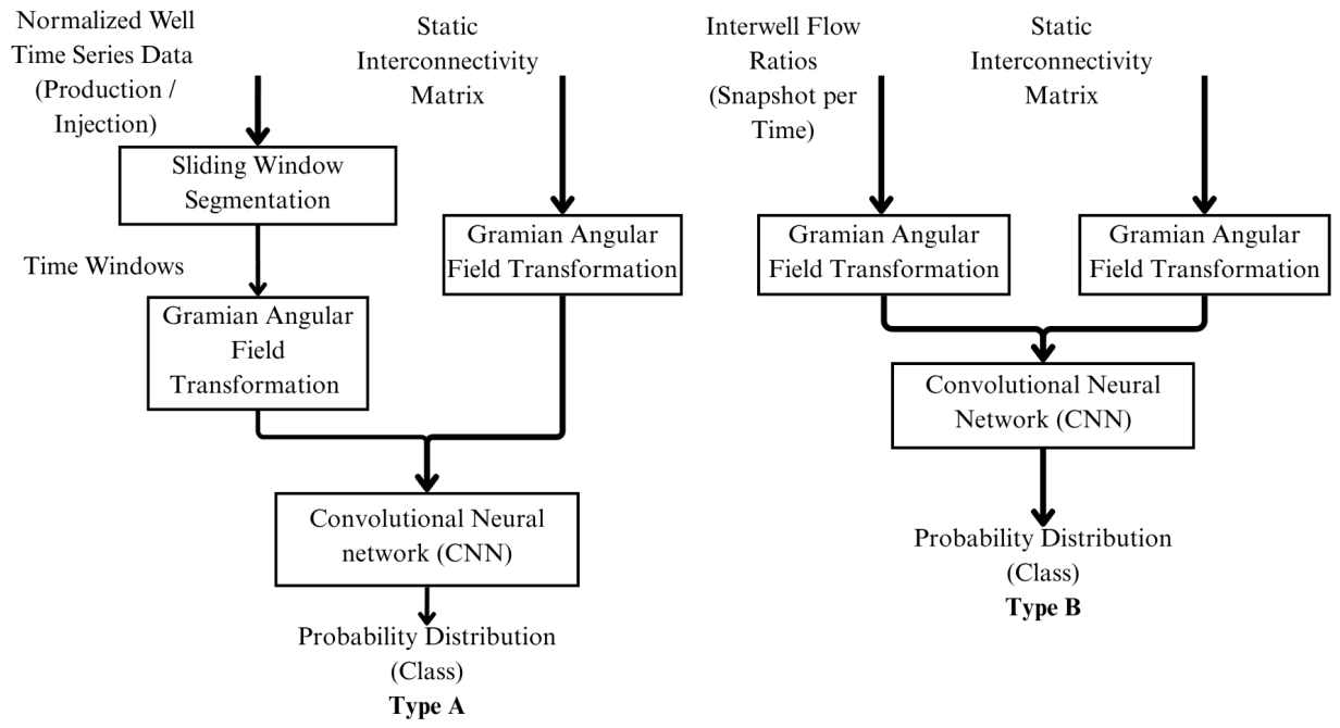
Figure 2.
GAF-to-CNN classification pipeline: a normalized time series is transformed into a GAF image, processed through convolutional and pooling layers, and passed to fully connected layers for final classification.
Figure 2.
GAF-to-CNN classification pipeline: a normalized time series is transformed into a GAF image, processed through convolutional and pooling layers, and passed to fully connected layers for final classification.
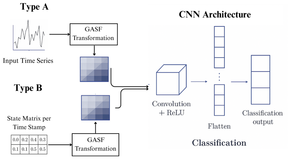
Figure 3.
Zone Probability Heatmap (Predicted) with Well Labels Type A. This figure interprets model predictions and visually emphasizes key spatial relationships that align with known or hypothesized interwell fluid-flow communication trends. Moreover, this visual output not only supports the validity of the model predictions but also offers intuitive interfaces for decision-makers to assess potential underground connections.
Figure 3.
Zone Probability Heatmap (Predicted) with Well Labels Type A. This figure interprets model predictions and visually emphasizes key spatial relationships that align with known or hypothesized interwell fluid-flow communication trends. Moreover, this visual output not only supports the validity of the model predictions but also offers intuitive interfaces for decision-makers to assess potential underground connections.
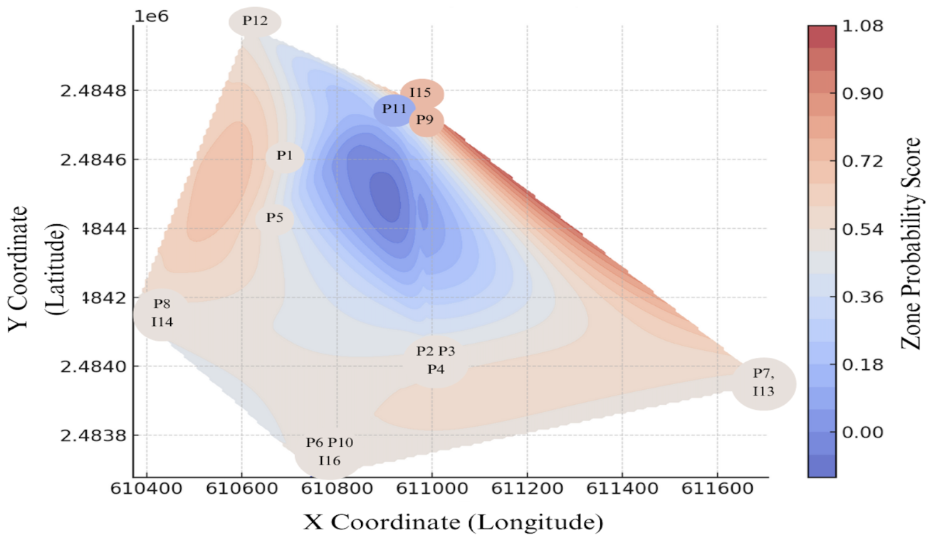
Figure 4.
Confusion Matrix for Zone Classification. Shows the model’s prediction accuracy per class. High values along the diagonal indicate strong performance, especially for Class 0 and Class 2. Displays prediction performance across all classes after augmentation. High diagonal values reflect strong classification accuracy.
Figure 4.
Confusion Matrix for Zone Classification. Shows the model’s prediction accuracy per class. High values along the diagonal indicate strong performance, especially for Class 0 and Class 2. Displays prediction performance across all classes after augmentation. High diagonal values reflect strong classification accuracy.
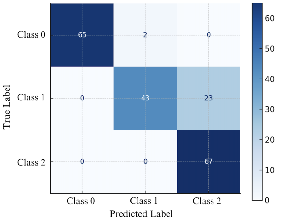
Figure 5.
Class Distribution After Augmentation. Displays the balanced dataset used for training and evaluation. All classes (0, 1, 2) are now equally represented, which helped mitigate model bias. Shows the post-augmentation balance across all three zone classes. This ensures fair training and evaluation, mitigating prior bias.
Figure 5.
Class Distribution After Augmentation. Displays the balanced dataset used for training and evaluation. All classes (0, 1, 2) are now equally represented, which helped mitigate model bias. Shows the post-augmentation balance across all three zone classes. This ensures fair training and evaluation, mitigating prior bias.
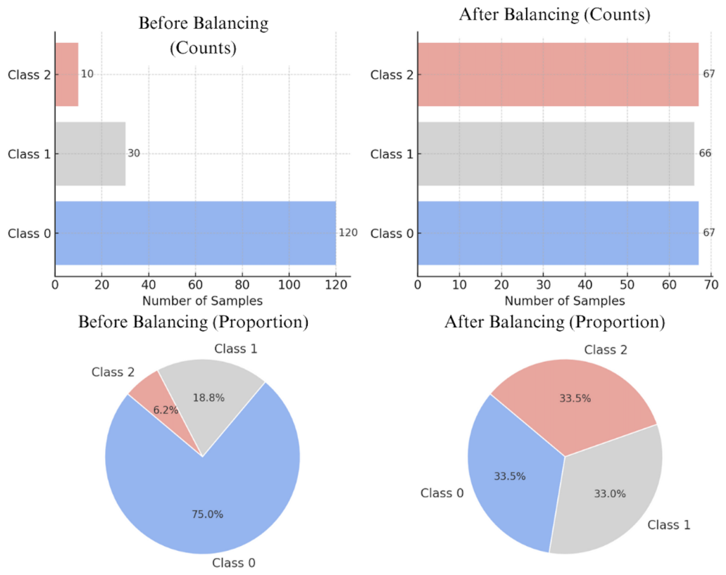
Figure 6.
Zone Class Heatmap by Well Location Type A.
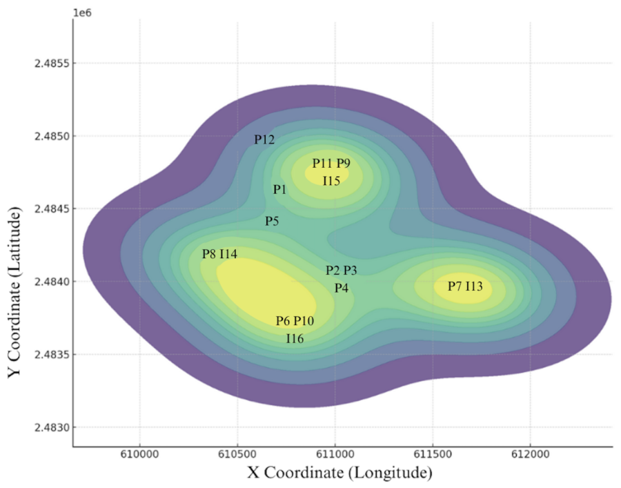
Figure 7.
Zone Class Heatmap by Well Location Type B.
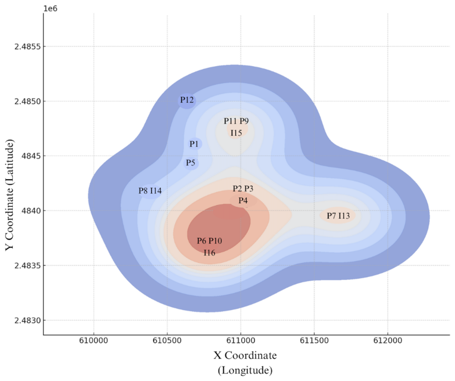
Figure 8.
Type B Zone Probability Contour. Interpolated spatial contour of zone scores predicted by the Type B model. Highlights well regions with a high likelihood of underground connectivity.
Figure 8.
Type B Zone Probability Contour. Interpolated spatial contour of zone scores predicted by the Type B model. Highlights well regions with a high likelihood of underground connectivity.
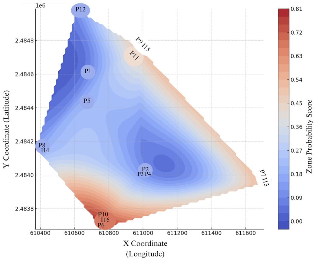
Table 1.
Comparison of Type A and Type B GAF Images
| Aspect | Type A GAF Images | Type B GAF Images |
|---|---|---|
| Source | Sliding windows of individual well time series | Per-timestamp flow interaction matrices across wells |
| Resolution | 30×30 grayscale images | 16×16 interaction maps transformed to 30×30 GAFs |
| Content | Single-well production/injection behavior | System-wide well-to-well interactions at each timestamp |
| Augmentation | Fourier + noise-based image generation | Fourier + noise-based image generation |
| Labeling | Based on well ID, then synthetically extended | Based on interaction matrix and zone classification |
| Use Cases | Regression, temporal clustering | Zone classification, probability scoring |
Disclaimer/Publisher’s Note: The statements, opinions and data contained in all publications are solely those of the individual author(s) and contributor(s) and not of MDPI and/or the editor(s). MDPI and/or the editor(s) disclaim responsibility for any injury to people or property resulting from any ideas, methods, instructions or products referred to in the content. |
© 2025 by the authors. Licensee MDPI, Basel, Switzerland. This article is an open access article distributed under the terms and conditions of the Creative Commons Attribution (CC BY) license.
Copyright: This open access article is published under a Creative Commons CC BY 4.0 license, which permit the free download, distribution, and reuse, provided that the author and preprint are cited in any reuse.


