
Submitted:
29 June 2026
Posted:
08 July 2026
You are already at the latest version
Abstract
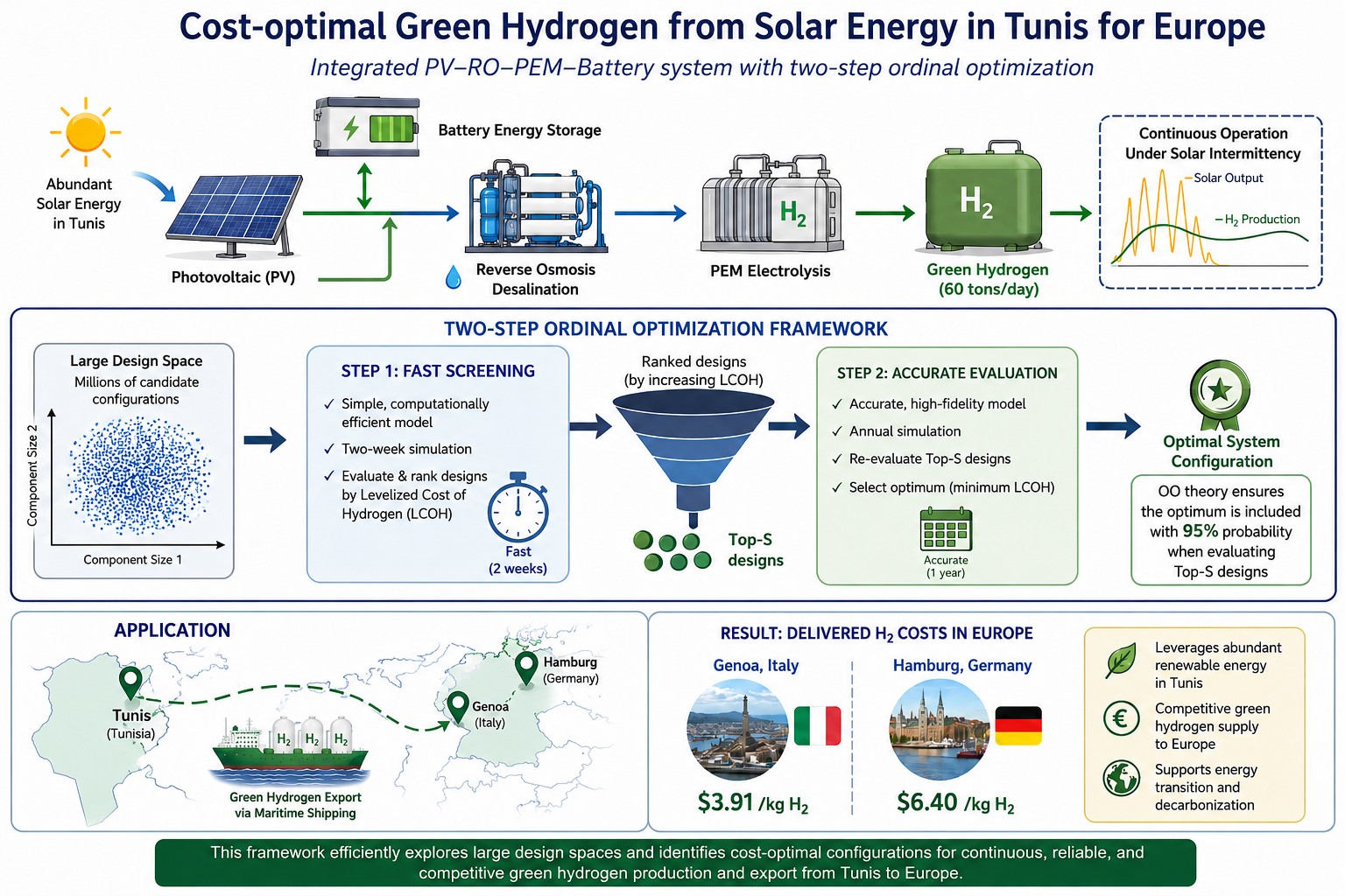
In this paper, we present an optimization framework for green hydrogen (GH) production integrating photovoltaic generation, reverse-osmosis desalination, proton exchange membrane electrolysis, and battery energy storage for continuous operation under solar intermittency. The study introduces a two-step ordinal optimization (OO) method to explore efficiently the large design space and identify subsystem sizes that minimize the levelized cost of hydrogen ($/kg), including production, storage, and transportation, at an average daily output of 60 tons of GH per day. First, the designs are evaluated using a simple, but computationally efficient model based on a two-week simulation. The evaluated designs are then scaled to a yearly operation and ranked by increasing hydrogen costs. Second, the top-S designs are re-evaluated using an accurate annual simulation model. OO theory predicts the number of top-S designs that need to be evaluated accurately to ensure that the optimum is included with a 95% alignment probability. We applied this framework to case studies for producing GH in Tunis and shipping it to Genoa in Italy and Hamburg in Germany, at costs of $3.91 and $6.40 per kg, respectively. The study leverages the potential of renewable energy (RE) production in Tunis and its proximity to Europe.
Keywords:
solar PV energy
; ordinal optimization
; water electrolysis
; hydrogen storage
; green hydrogen shipping
; cost of green hydrogen production
1. Introduction
The transition to clean energy is essential for improving the quality of life and meeting environmental goals, but rising energy demand has intensified the reliance on fossil fuels, which has increased CO2 and other harmful emissions. Green hydrogen, produced from low-carbon sources, offers a strong pathway to net-zero by 2050. Its production enhances renewable energy usage, helps in stabilizing the grid through cleaner energy, and reduces emissions in industry, transportation, and heating. Countries like Germany and the UK are already adopting it in sectors such as steelmaking and residential heating [1].
Hydrogen production is mostly fossil-based, with renewable electrolysis representing a small fraction. Green hydrogen (GH) can reduce CO₂ emissions and support renewable integration but remains costly, requiring production scaling and techno-economic optimization. Its role in decarbonizing hard-to-electrify sectors and enabling large-scale energy storage makes GH strategically important for low-carbon energy production systems [2]. Significant advances in hydrogen technologies are accelerating the clean energy transition; by 2050, hydrogen could supply nearly half of the EU’s energy demand, requiring 3,100 to 6,000 TWh annually. Large projects like the Neom Green Hydrogen Project —targeting 650 tons/day by 2025— are expected to reduce CO₂ emissions by about 3 million tons per year and support the growth of a sustainable global hydrogen economy [3]. EU green hydrogen demand is expected to exceed domestic production, making imports essential, with Africa being a well-positioned key supplier due to its abundant renewable resources and proximity. Germany anticipates a substantial shortfall by 2030 —consuming 110 TWh but producing only 14 TWh— driving significant imports and €2 billion in global GH investments. These trends highlight hydrogen’s increasing strategic role in the energy transition for both Africa and Europe [4].
Researchers highlighted GH’s vital role in decarbonizing power and industrial sectors. Goldmeer et al. [5] reported that GE is advancing hydrogen turbine technology to facilitate the transition toward zero-carbon energy, while Rubio et al. [6] emphasized that meeting climate goals requires a decarbonized economy. Using an optimization model, they estimate Spain’s hydrogen demand for replacing conventional vehicles by 2030 and determine the electricity needed for GH production. They found that the estimated production costs using wind, solar PV, and hydropower are 81.37, 81.65, and 68.12 €/MWh, respectively. Based on the lower heating value (LHV) of hydrogen, these costs correspond to 3.15, 3.16 and 2.63 $/kg. Kakoulaki et al [1] found that most EU27 and UK regions could generate sufficient renewable electricity (290 TWh) to replace grey hydrogen with GH, which supports EU energy policy and emphasizes the need for further research on regional systems and hydrogen infrastructure.
Ayres et al. [7] highlighted that PEM electrolyzers efficiently produce hydrogen, but high electricity usage and costly components—such as iridium catalysts and thick membranes—keep costs well above the $1/kg target, highlighting the need for technological improvements. Asaad and Karaki [8] evaluated a North African GH production plant using solar PV, seawater desalination, PEM electrolysis, and battery storage. Using Tunis weather data, they estimated a levelized cost of hydrogen (LCOH) at $6.43/kg by 2030, falling to $3.81/kg by 2050, suggesting improved competitiveness with carbon taxes. Alghool et al. [9] applied a mixed integer linear programming (MILP) model to optimize green hydrogen production in Qatar using PV/PV-T collectors and alternative water sources. PV-T dominated the hydrogen output, while treated sewage effluent was a preferred water source, with oxygen sales enhancing revenues. The LCOH was most sensitive to demand, PV-T costs, and oxygen prices, while carbon taxation had minimal design impact. Hussam et al. [10] evaluated green hydrogen production at the Shagaya Renewable Power Plant in Kuwait. Results show that a grid-connected PV–wind configuration is the most cost-effective, while stand-alone systems are economically less attractive, with system performance strongly influenced by PV costs. Rodrigues Vaz et al. [11] presented the design of a photovoltaic-based green hydrogen production plant in Ceará, Brazil, using the Systematic Layout Planning method to optimize equipment layout, production flow, and operational efficiency. The results confirm the technical feasibility and potential of large-scale green hydrogen production in Brazil with some limitations.
Hydrogen storage and transportation may be realized as either gas under very high pressure or in liquified state. Rong et al. [12] compared hydrogen storage and transport options, concluding that compressed hydrogen is best for short distances and small volumes, while liquid hydrogen and liquid organic hydrogen carriers (LOHC) are preferable for long-distances, and large-volume transport. LOHCs are particularly efficient for daily demands above 20,000 kg, and pipelines are effective for short, high-volume routes under 100 km. Storage tank materials have been studied and thoroughly tested during filling and emptying. De Miguel et al. [13] demonstrated that Type IV hydrogen tanks experience higher temperature rise and stronger temperature stratification during use, while Type III tanks enable faster and safer filling due to the aluminum liner’s quicker thermal response, which also improves gas temperature monitoring. Ye and Lu’s [14] life-cycle analysis showed that Type IV hydrogen tanks have the lowest emissions and lowest cost ($10.4/kg H₂), outperforming Type III and cryogenic tanks, and making them the most efficient and practical option for hydrogen transport. The geometry and the mass of different storage tanks and their thermal response were investigated by Klymyshyn et al. [15], who developed a tool to estimate the geometry, mass, and cost of Type III and IV hydrogen tanks with about ±10% accuracy, helping assess storage feasibility for mobile and stationary systems.
The shipping of GH and its transportation cost is presented by Alkhaledi et al. [16] through “Jamila”, a 370 m liquefied hydrogen (LH) tanker with a 230,000-ton displacement, carrying 20,000 tons of LH and reaching 19 knots with a 50 MW gas turbine engine. Its low deadweight, draft, and high freeboard result from hydrogen’s low density, giving it characteristics similar to LNG carriers. They report that a 280,000 m³ LH tanker offers strong long-term financial viability, achieving a 45.1% IRR at a hydrogen price of $2/kg in 2040 [17]. Kassembe and Gang [18] showed that ship costs decrease with size as capital costs fall from $7,200 to $3,600 per DWT for 50,000 to 200,000-ton vessels, and operating costs, excluding fuel, drop from $30,000 to $11,000 per DWT per year. However, as larger ships benefit from economies of scale, they are less suitable for short-distance routes.
Optimization is commonly applied in engineering design to size system components for minimum cost and yet feasible operation. Ordinal optimization (OO) [19] is a very efficient meta-heuristic technique that formulates the problem as a search in a large design-space through simulation to identify the best design based on ranking or “order”. Jabr and Pal [20] applied OO for distributed generators (DG) placement and sizing, achieving reliable results with lower computational effort than stochastic or other meta-heuristic methods. Karaki et al. [21] used OO to optimize the sizes of subsystems in a fuel cell hybrid electric vehicle, showing significant benefits in hydrogen savings and in car performance. Both studies highlight OO's potential for solving complex energy problems efficiently. Dias et al. [22] applied Genetic Algorithms to optimize the Celza GH network, projecting 3.1 to 7.7 TWh demand by 2030 and about 1 Mt CO₂ reduction annually, while showing that the project could remain economically viable with only one-third of the planned 5.5 GW electrolysis capacity.
This paper presents a novel framework based on ordinal optimization (OO) to find the optimal design of a green hydrogen production plant in North Africa (NA) for local use, or for shipping to Europe. It involves simulating the operation of the green hydrogen production system with six subsystem sizes of a photovoltaic (PV) plant, a reverse osmosis (RO) plant, a PEM water electrolyzer, battery energy storage, hydrogen compression pressure, and hydrogen storage for local use, or ships for transportation to Europe. The great merit of this approach is to enable the finding of a really “good-enough” design, very efficiently, using operational simulation only. This simulation is enabled using an energy management system (EMS) to integrate the operation of the different subsystems under daily and seasonal solar radiation variations. The goal of the EMS is to ensure that operation is feasible within the specified subsystem sizes. When operation of a design is feasible, the annualized capital and operational costs are calculated and divided by the annual hydrogen production to deduce the levelized cost of hydrogen (LCOH) in $/kg for the design being evaluated. However, if operation is not feasible for a given design, a penalty is added to the operational cost of the design in question, and the LCOH becomes higher making its selection less likely as a really good-enough design. This is a combinatorial problem to find an optimal design in a relatively large search space. When seven sizes for each of the six subsystems are defined, the search-space has 279,936 () possible designs, which for combinatorial problems is not a very large space. When these designs are evaluated using an accurate model by directly simulating the yearly operation of all designs, this would take 58,554 seconds or about 16 hours. While such evaluation seems achievable, its utility is significantly compromised when designing a system, as the bounds of the search space may need to be modified. If an optimum design is at one of the bounds of the search space, then the bound in question needs to be relaxed, and all the designs are to be reassessed. When designing the system, this reassessment may occur several times in some iterative way. A wait of 16 hours by the designer, at every modification and reassessment, makes the use of such a tool rather impractical and burdensome.
To overcome this limitation, we propose to use the OO approach to evaluate the designs in two steps: in the first step we evaluate all the designs using a simple but computationally efficient model that simulates the operation over a two-week period representative of the seasonal solar energy variations. The evaluated designs are then ordered in ascending hydrogen-cost. However, due to the use of a simple model, noise is introduced in the ordering, but order is robust to the noise introduced [19]. Furthermore, OO theory predicts the number of top-S designs that we need to re-evaluate in order for the optimum design to be included with a high-alignment probability. The operations of the top-S designs are simulated over a full year and the best among them is selected. This two-step process would typically take 37.6 minutes, for the above-described case. Thus, the waiting-time for any reassessment falls well within normal expectation of finding a “really-good” design with a high probability of being the optimal. The use of simulation to find the optimum design is in some respect similar to genetic-algorithms (GA), however, the OO approach is computationally much more efficient, and its solution is repeatable and tractable. When using GA to find the optimum design of the above search space, with a population of 100 and running over 150 generations, it would require 15,000 evaluations, which would require about 52.3 minutes. This is higher than the time needed for the two-step OO process of about 37.6 minutes. The effectiveness and versatility of the developed tool are demonstrated through its use to carry out three case studies: (i) green hydrogen production and storage for local use, (ii) production and maritime transport from Tunis to Genoa, and (iii) production and transport from Tunis to Hamburg. The results confirm that the proposed OO-based methodology provides a practical, computationally efficient, and scalable decision-support tool for large-scale green hydrogen system design under realistic conditions.
2. Problem Formulation
A system’s overview of the green hydrogen (GH) production plant in North Africa (NA) is shown in Figure 1. GH is produced for either local storage or for shipment by sea to Europe. The PV plant generates electric power for a PEM electrolyzer to separate water into hydrogen and oxygen. A reverse osmosis (RO) plant desalinates seawater to produce freshwater and feed it to the electrolyzer. The battery system supports continuous PEM hydrogen production, especially at night albeit at lower output rate, and is fully recharged by the solar panels in the day. GH may be used locally or transported to Europe via ships equipped with hydrogen Type IV containers, at very high pressures. Two shipping by sea case-studies are conducted: the first has a sea-distance of 856 km from Tunis to Genoa, Italy; the second has a sea-distance of 4350km from Tunis to Hamburg, Germany.
The objective is to determine the sizes of the plant subsystems that lead to a minimum hydrogen cost, in $/kg, for production and delivery. The sizes are those of the PV plant, the battery system, the PEM plant, the RO plant, the hydrogen storage, and its pressure, or the size and number of ships to transport GH to Europe. The different subsystem sizes define N designs over which the cost function φ (in $/kg) is minimized:
The annualized capital cost , the annual operation and maintenance cost , and the annual hydrogen production are evaluated for each design vector: [PV, PEM, RO, BT, PR, ST or SH] where the elements are the sizes of the subsystems.
3. Subsystems’ Modeling
3.1. PV Plant Model
The PV plant model determines the electricity generated by a set of panels, under varying solar radiation and temperature conditions. We first calculate the cell temperature (), which depends on ambient temperature () and solar irradiance (), as follows: , where and is the nominal operating cell temperature, which is determined under manufacturer test conditions at an ambient temperature of 20°C; a typical value of is 46°C. At a solar irradiance , the short-circuit current and open-circuit voltage of the module are calculated as:
To determine the average hourly power output under operating conditions, we note that the ratio of the voltage at maximum power () to the open-circuit voltage () remains nearly constant as solar conditions change. Similarly, the ratio of the maximum-power current () to the short-circuit current () also remains nearly constant. From this observation, we can express the maximum power at the current field conditions as a function of the maximum power at STC, as follows:
The annual PV energy is calculated by integrating hourly maximum power values (). Using the number of modules per design and module characteristics, the total PV plant capacity is determined, allowing us to estimate its investment and operational costs.
3.2. RO Plant Model
The RO plant is modeled based on the “Constant Water Recovery Rate” method outlined by Zein et al. [23]. For a daily hydrogen production target of 60 tons, the corresponding water requirement is 540 tons/ day based on the molecular weight ratio of 1:9. This approach keeps the RO recovery rate constant while permitting variations in feed pressure and flow rates to adapt to changes in available power. The fixed RO recovery rate operation, shown in Figure 2, offers greater operational flexibility compared to the fixed feed pressure method recommended by RO membrane manufacturers.
The high pressure (HP) pump is controlled to supply the net RO feed flow at the required pressure, while the booster pump manages the energy recovery device (ERD) flow to recover the pressure in the concentrate stream.
3.3. PEM Plant Model
To determine the power required by the PEM system, a function is developed to account for the hourly hydrogen production rate, system efficiency, current density, and voltage per cell. The PEM electrolyzer’s cell voltage () depends on three main voltage components [24]: the ohmic voltage (Voℎm), representing internal losses, the activation voltage (Vact), required to trigger the reaction, and the Nernst potential (Ecell), which is the minimum voltage needed to split water molecules:
The electrolyzer output voltage , of a stack of series cells, is given by:
The total operating current () of parallel stacks each of series cells is directly related to the hydrogen demand (kg/s) as follows:
The Faraday constant is equal to 96485 C/mol, is the flow rate of hydrogen (kg/s), and is the hydrogen molecular weight (g/mole), and is the Faraday efficiency. The number of parallel PEM stacks in each design is specified, and the cost of investment can be determined, while the number of cells in series per stack is constant as determined by the specified operating voltage of the PEM electrolyzer. The power required by the electrolyzer () is given as:
where is the ratio of auxiliary to output power.
3.4. Battery Storage Model
Energy storage is provided by batteries that are charged during the day from the solar PV plant to continue hydrogen production at night, however at a lower rate. The storage size is defined by the number of parallel battery strings, and the simulation checks whether this configuration can provide reliable charging and discharging. Each string contains 500 series battery cells. The battery voltage (), and its resistance are given by:
The state of charge (SOC) of the battery is monitored hourly to determine whether it requires charging when sufficient solar energy is available to keep its SOC below the maximum threshold. Additionally, the battery SOC should be evaluated to ensure that it exceeds the minimum level of 20% when it is required to supply power. The SOC at time is calculated as follows:
Here, Pbat represents the power output of the battery, which is positive when discharging, Ploss denotes the power loss of the battery, Q(t) is the internal energy of the battery at time t, and Emax is the energy capacity of the battery. The power delivered by the battery is , and so Ploss is given by:
3.5. Hydrogen Compression Model
A hydrogen production system also needs a compressor to prepare hydrogen for storage or transportation. The power required by the compressor is given by [25]:
= 30 bar is the inlet pressure of the compressor, which is fed from the electrolyzer, is the outlet pressure of the compressor, which is the tank pressure calculated using the Redlich-Kwong real gas equation, is the hydrogen compressibility factor of 1.032, is the number of compressor stages, assumed to be 2, is the inlet temperature of the compressor taken as 311 K, is the specific heat ratio equal to 1.4, is the molecular weight of hydrogen in g/mol, is the compressor efficiency taken as 75%, and is the universal gas constant. Hydrogen is compressed and stored in tanks, with a tank capacity determined by a specified number of production days for accumulation.
When transported to Europe, the hydrogen storage system essentially consists of large ships, with on-board storage with pressures ranging from 250 to 500 bars. The total power consumption given by Eq. (15) is integrated over time to calculate the annual energy of the compression process.
4. Scenarios of Green Hydrogen Production
Two scenarios of green hydrogen production are considered. The first is a local use scenario where the GH is compressed and stored for domestic use in Tunis. For each design for this scenario, the subsystem specifications include the storage tank pressure and size, and based on this the total capital, operation and maintenance costs are evaluated. The second scenario considers shipping to Europe, where GH is produced in Tunis and transported to Europe, and total costs are calculated based on ship capital cost, compression cost, and shipping expenses, considering different ship sizes and storage pressures that depend on destination.
4.1. Green Hydrogen for Local Use
The approach uses the geometry, capacity, and material cost of Type IV pressure vessels. The storage tank prototype is modeled after Provaris' H2Neo [28] compressed hydrogen carrier. The critical dimensions of the Type IV storage tank are the inner radius and inner length , see Figure 3. The Type IV tank features a high-density polyethylene (HDPE) nonmetal liner and a composite carbon fiber (CCF) over-wrap [12]. The liner thickness is determined as follows:
The factor = 0.04/250 is the ratio of the liner thickness to the internal length [25]. In Figure 3, the blue part represents the thickness of the HDPE liner, and the gray part is the CCF thickness. The wall thickness () of a Type IV storage tank depends on the internal pressure and the inner radius () and is given by [15]:
is a safety factor of 2.25, is the fiber translation efficiency that serves as a parameter to represent the disparity between the theoretical and the practically achievable strength of carbon fiber, its value ranges from 75-85 %, is the maximum internal pressure of the tank (bars), and is the pressure design strength of the carbon fiber laminate in the hoop direction equal to 15,300 bars [15].
The strength of the composite wall in the hoop direction is based on a laminate structure, with about two-thirds of the fibers-oriented hoop-wise and one-third axially. Carbon fiber vessels are fabricated with fiber tows in crossing helical patterns, which approximate the 1/3 axial and 2/3 hoop distributions. The tank volume () is given by:
The weight of the materials for the CCF and HDPE liner is computed from their respective volumes as follows. The volume of the liner is estimated by:
The liner radius and mass are, respectively, estimated by:
is the density of the liner equal to 1370 kg/m3. The same process is applied for the CCF wrapping, whose thickness is:
is calculated using Eq. (17), and the CCF mean radius is determined by:
The volume of the CCF wrapping and its mass are respectively given by:
The density of the CCF wrapping with resin is equal to 1580 kg/m3 [29]. The mass of the storage tank is given by:
The size of the GH storage for days of production is determined as follows:
is the size of the GH storage (kg), is a capacity factor of about 0.55, based on a one-year simulation, which represents the proportion of hydrogen actually produced and stored as compared to the electrolyzer's production capacity of (kg/day), is the number of storage days. Consequently, the volume of GH storage () is given by:
is the density of at the nominal tank pressure. The number of storage tanks needed is then calculated as follows:
The total mass of the tanks ) on a ship in kg is given by:
The total cost of the storage system can then be determined as follows:
4.2. Shipping Green Hydrogen from NA to Europe
This scenario examines transporting gaseous GH from Tunis to Genoa and from Tunis to Hamburg. The specialized vessels used in this study are based on the Jamila and Provaris H2Neo designs. The water displacement of a GH ship () in tons, is obtained using the following relation based on the evaluation of Jamila’s fully loaded displacement tonnage [16]:
Where is the ship water-line length (m), is the width of the ship(m), is the draft of the ship at full load (m), is the block coefficient at full load, and is the Mediterranean seawater density of about .
The pressure-tank design begins by defining the base geometry—its internal and external shape—followed by calculating the wall structure needed to withstand internal pressure. Type IV cylinders are also chosen for transporting gaseous green hydrogen. A cylindrical tank with uniform wall thickness and hemispherical end caps is assumed, which is used to estimate the cost of the Type IV storage tank. The ship’s hydrogen tank geometry is determined using standard storage-tank equations used in the Local Use Scenario, however with different dimensions. Since the ship carries two Type-IV tanks, the total tank mass and the mass of hydrogen transported per ship are given, respectively as follows:
is the density of hydrogen at the selected hydrogen pressure.
The cost of a Type-IV hydrogen tank varies with its size and material mass. Using data by Karayel et al. [26], a lookup table is created to link tank mass (kg) to the specific tank cost ($/kg) across pressures from 100 to 1000 bar, as shown in Figure 4. The cost of our ship’s prototype storage tanks, as follows:
The factor of 0.9 accounts for the balance of plant cost [27], and is the unit cost of a tank ($/kg).
The unit cost of container ship is a critical factor to consider, which is expressed usually in USD per ton, since the focus is on dry bulk shipping data analysis. Kassembe and Gang [18] established a relationship between the new building container ship and its deadweight tonnage. Based on this, the ship hull capital cost ($) can be calculated using the following equation.
Where is the ship-hull unit cost ($/kg), is the mass of the water displacement of the hydrogen ship (tons), and is the mass of the two hydrogen tanks when full. To sustain the greenness of hydrogen, the ships are assumed to be hydrogen-powered, which is a promising clean solution for maritime transport, producing minimum direct NOx, SOx, or particulate emissions [26]. The ship engine is driven by hydrogen using fuel cells and batteries, and its size is as follows:
is the engine size (MW), and (MW/ton) is the ratio that relates the engine size (50 MW) of Jamila LH2 tanker to its water displacement of 230,000 tons [16].
5. Ordinal Optimization
When searching for an optimal solution in a large search space of designs, Ordinal Optimization (OO) is a method that makes use of two key principles [19]. First, we note that "order" is less sensitive to noise than "value," and second, rather than aiming to find the “optimum” solution, we aim for "good-enough" solutions with a high alignment probability of being the optimum, which is known as goal softening. The OO process first uses a simple, efficient simulation to rank designs by cost, identifying the really “good-enough” designs at the top of the list. A subset of these designs is then reevaluated with an accurate model to reduce noise, and the top design from this reduced list has a high alignment probability of being the optimal. This is known as a horse-race approach that is effective for complex systems with non-linearities and discrete variables and outperforms the blind pick selection method.
For our problem, let represent the search space of the optimization variables, which are the sizes of hydrogen production subsystems. Let denote the set of designs that are uniformly sampled from the search space . When is large (e.g., = 1000 or more), the selected is considered to represent the total search space . Let represent the “good enough” subset within , also referred to as the top-g designs, which would include the optimum design. Let be the subset consisting of the top-s designs from then the best design of is highly likely to be part of . So, the designs belonging to and , or form a set of “truly good-enough” designs within with a high alignment probability of being the optimum. This is mathematically expressed as 0.95, which is the probability that there is at least truly good enough designs in , where is the alignment level. The OO theory [19] predicts the size of the selected subset using , with , = 8.1998, = 1.9164, = -2.0250 and = 10. The size of is found to be 12, which means that we need to evaluate the first 12 designs using the accurate model, to remove the error introduced through the use of a simple model, of and select the best among them, with a probability of 95% of being the optimum. The coefficients are obtained from a table of regression coefficients, developed for a large set of problems for an = 0.95 [19]. They correspond to a low error bound of = 0.5 per unit, since our simple model yields results that are rather close to those of the accurate model for operating cost, energy production, and utilization. Figure 5 shows a flowchart of the OO process, outlining the steps for identifying a “truly good enough” design with a 95% probability of being the optimum.
The design of the GH production and shipping process is evaluated by simulation using the developed models in Sections IV and V, which are integrated using an energy management system (EMS) to create a comprehensive simulation for the operation of the GH plant. The logic of the EMS is shown in Figure 6, as upgraded from an earlier version [8]. We first forecast the daily energy produced by the PV plant, then we schedule hydrogen production of the PEM plant, which is followed by the water production of the RO unit and energy required for compressing GH into the storage. Excess energy of the PV plant is used to charge the batteries to maintain operation when solar energy is unavailable. The PEM electrolyzer operates at two levels: a higher output during the day and a lower output at night. The daily hydrogen production follows the forecasted daily solar energy of Tunis, with an adaptive method to adjust the schedule based on actual solar conditions. Production is raised when sufficient solar energy is available and the battery SOC increases, and it is reduced when the battery SOC decreases.
The simulation model evaluates the designs to estimate the specific cost of hydrogen production for each. The simple model of the OO process simulates the operation of the plant over two weeks, or 336 hours, and then scales it to one year for energy utilization and cost assessment. Given that the year has 8760 hours, the number of simulations is thus reduced by a factor of 26.
6. Results and Discussion
This study explores the design of a solar-powered GH production plant with an output of approximately 60 tons per day. The plant’s capacity is determined based on annual solar radiation data for Tunis. The overall cost function, Eq. (1), includes the annualized capital cost for each design corresponding to a set of subsystem sizes of the GH plant, and the operation and maintenance (OM) costs . The OM costs are estimated at 2.0% annually of the investment for all subsystems except for the PV plant that has an OM cost of 1.5% annually. For the economic analysis, a system lifespan of 20 years was assumed, along with an interest rate of 7%. Table 1 outlines the cost parameters for the primary system components. The cost of the PV solar system [30] includes inverters, structural supports, and installation.
6.1. Local Use Scenario
In the local use scenario, the simple model of the OO platform evaluated 1,152 design options in 9.9 seconds. The different subsystem sizes used in the designs are specified in Table 2. The top 20 designs are listed in Table 3, which use a 500-bar hydrogen storage pressure. The ordered performance curve of the best 140 designs is shown in Figure 7.
The running of the accurate model for the top-20 designs took 4.5 seconds to identify the optimal design, which ranked 8th in the simple model evaluations. The top three designs are summarized in Table 4, with annual PV energy production and subsystem energy consumption.
6.2. Tunis to Genoa Shipping Scenario
Using the same computational model, we investigated the production of GH in NA and its shipping to Europe in two case studies: Tunis to Genoa, and Tunis to Hamburg. The Tunis to Genoa route has a sea distance of 856 kilometers, which is covered by our ship model at a speed of 41.5 km/h or 22.5 knots. The one-way trip takes about one day, with docking and unloading lasting 2.86 days for each. The OO platform simulated 1,152 designs shown in Table 5, using a two-week simple model in 9.7 seconds, estimating annual production costs. The top 20 designs, all at 500 bars, are shown in Table 6.
The accurate model took 4.5 seconds to evaluate the 20 top designs and identify the optimal design that ranked 9th in the simple model. The top three designs are summarized in Table 7, with annual PV energy production and subsystems’ energy consumption. The optimal setup for GH transport to Europe requires three 120-meter ships completing a total of 220 trips per year.
6.3. Tunis to Hamburg Shipping Scenario
The shipping distance from Tunis to Hamburg is approximately 4,350 km. Transporting over this distance with a ship travelling at 41.5 km/h (22.5 knots) requires a one-way journey of about 5 days, and an additional 3.42 days for each of the filling and unloading of a ship. Here we use the same subsystem sizes as in Table 5 but choose the last row for the ship sizes and numbers. The simple model simulated all 1,152 design options over two weeks in 9.61 seconds.
Table 8 lists the top 20 designs with all having a storage pressure of 500 bars as obtained by the simple model. Running the accurate model for these top 20 designs took 4.94 seconds and identified the optimal design, which ranked seventeenth in the simple model evaluation. Table 9 summarizes the characteristics of the top three designs, with energy flows. The optimal design produces 23,285 tons of hydrogen annually, at an average of 63.8 tons/ day, and has a delivery capability of 23,114 tons annually yielding a production and shipping cost of $6.401/kg.
In seeking the optimum design of this case study, we first used the same shipping infrastructure of the Tunis to Genoa case study. However, the tool informed us that the hydrogen delivery capability is significantly less than its annual production, which indicates that we needed to repeat the search with an increased shipping infrastructure as shown in the last row of Table 5. Let us note that the mismatch between the delivery capability and the annual H2 production is now reduced. It may be further reduced by using a smaller PV plant of 855 MW instead of 870 MW, which would produce slightly less hydrogen, however at the lower cost of $6.375 per kg. This shows that the developed tool is useful in fine tuning the boundary of the search space for the benefit of cost reduction.
6.4. Validation
The model was validated by comparing its results with existing studies. For the optimal designs, presented in Table 4, Table 7 and Table 9, the average specific energy consumption is 55.2 kWh/kg H₂ for PEM electrolysis, 4.56 kWh/m³ for the reverse osmosis system, and 2.49 kWh/kg H₂ for compression. Table 10 shows that specific energy consumptions across subsystems are well within the ranges of previous studies, which provides validation of the mathematical models used.
To validate the ordinal optimization (OO) method, an exhaustive search was carried out on the sampled space of 1152 designs, as applied to the local use and shipping scenarios. As shown in Table 11, the OO method substantially reduced computational time while maintaining very good solution quality. It identified the same optimal designs as the exhaustive search for the local-use and the Tunis-Hamburg scenarios and a second-best design for the Tunis-Genoa scenario, demonstrating its effectiveness in efficiently exploring large design spaces with minimal computational effort.
7. Conclusions
This paper proposes a design methodology combining detailed simulation and Ordinal Optimization (OO) to minimize the cost of large-scale GH production in North Africa. Solar-powered desalination and PEM electrolysis were used to produce hydrogen that is stored at high pressure for local use or for maritime shipment to Europe. Battery storage ensures continuous operation, and the approach optimally sizes PV panels, batteries, desalination units, electrolyzers, storage tanks, and shipping to achieve about 60 tons of hydrogen per day at minimal cost. The large search space, is formed of designs with the different combinations of subsystem sizes; it is first efficiently screened using a simple-model based on simulating system operation over a two-week period. Their yearly hydrogen production costs are then estimated through scaling, and the designs are ranked in increasing cost. The top-S designs are then evaluated using an accurate model based on a full-year simulation to determine their hydrogen production costs and identify the top design, with a high alignment probability of being the optimum.
Two main scenarios were explored in this study: the first is for local hydrogen utilization in North Africa, where the GH produced is stored in type IV storage tanks; the second is to export GH to Europe through maritime transportation. In the local-use scenario, the OO technique identified an optimal configuration with a hydrogen production and storage cost of $2.966/kg H2. This optimal system consisted of a 930 MW PV plant, 1728 MWh of battery storage, a 102-ton/day PEM electrolyzer, and a 56.25 m³/h RO desalination unit. This setup achieved a daily hydrogen production of 66.5 tons/ day and required 229 type-IV storage tanks with a capacity of 267 tons.
Two case studies were conducted to illustrate the export scenarios. The first is a system to exporting GH from Tunis to Genoa: the optimal design consisted of 900 MW PV, 1728 MWh battery storage, a 110 ton/day electrolyzer, 56.25 m³/h RO capacity, and three 120-meter ships each with a storage of 111 tons of GH at 500 bars, making 220 trips annually. The cost of production and transport is estimated to be $3.909/kg H2. The second case study is to transport GH from Tunis to Hamburg, which consisted of 870 MW PV, 1728 MWh of battery storage, a 107 ton/day PEM electrolyzer, 56.25 m³/h RO capacity, and six 130-meter ships each with a capacity of 141 tons at 500 bars. The ships need to make 169 trips per year, with a cost of GH production and transportation of $6.401/kg H2. Overall, the results highlight the effectiveness of integrating simulation with ordinal optimization for designing cost-effective green hydrogen production and distribution systems suited to both local usage and export destinations.
Author Contributions
“Conceptualization, S.K.; methodology, A. A.; software, S.K. and A.A.; validation, A.A; formal analysis, S.K. and A.A.; investigation, A.A.; resources, S.K.; data curation, A.A.; writing—original draft preparation, A.A; writing—review and editing, S.K. and A.A.; visualization, S.K. and A.A.; supervision, S.K.; project administration, S.K.; funding acquisition, S.K”. All authors have read and agreed to the published version of the manuscript.
Data Availability Statement
Data will be provided upon request.
Acknowledgments
The authors thankfully acknowledge the support of the work described in this article through the PhD program at the Maroun Semaan Faculty of Engineering and Architecture of the American University of Beirut, Lebanon. The solar irradiance data used was obtained through the EU funded project “Optimal Engineering Design for Dependable Water and Power Generation in Remote Areas Using Renewable Energies and Intelligent Automation - Open Gain”, proposal No. 032535, FP6-2004-INCO-MPC-3. The project was led by Professor Essam Badreddin of Heidelberg University, Germany. This paper reflects only the views and opinions of its authors.
Conflicts of Interest
The authors declare no conflicts of interest.
Abbreviations
The following abbreviations are used in this manuscript:
| GH | Green hydrogen |
| OO | Ordinal optimization |
| LOCH | Levelized cost of hydrogen |
| MILP | Minimum integer linear programming |
| LOHC | Liquid organic hydrogen carrier |
| LH | Liquified hydrogen |
| DG | Distributed generator |
| FCHEV | Fuel cell hybrid electric vehicle |
| NA | North Africa |
| PV | Photovoltaic |
| RO | Reverse osmosis |
| PEM | Polymer electrolyte membrane |
| EMS | Energy management system |
| GA | Genetic algorithm |
| ERD | Energy recovery device |
| SOC | State of charge |
| HDPE | High density polyethylene |
| CCF | Composite carbon fiber |
| CF | Capacity factor |
| AP | Alignment probability |
References
- Kakoulaki, G.; Kougias, I.; Taylor, N.; Dolci, F.; Moya, J.; Jäger-Waldau, A. “Green hydrogen in Europe – A regional assessment: Substituting existing production with electrolysis powered by renewables”. Energy Convers. Manag. 2021, Vol. 228, 113649. [Google Scholar] [CrossRef]
- Terlouw, T.; Bauer, C.; Mckenna, R.; Mazzotti, M. “Large-scale hydrogen production via water electrolysis: a techno-economic and environmental assessment”. Energy Environ. Sci. 2022, 15, 3583–3602. [Google Scholar] [CrossRef]
- Scita, R.; Raimondi, P. P.; Noussan, M. Green Hydrogen: The Holy Grail of Decarbonization? 2020. Available online: https://ssrn.com/abstract=3709789.
- Federal Ministry for Economic Affairs and Energy, The National Hydrogen Strategy; Federal Ministry for Economic Affairs and Energy: Berlin, 2020.
- Goldmeer, J.; Catillaz, J.; Donohue, J. “Hydrogen as a fuel for gas turbines A pathway to lower CO2”. 2021. Available online: https://www.gevernova.com/gas-power/future-of-energy/hydrogen-fueled-gas-turbines.
- Rubio, F.; Albert, C.; Jos’e Besa, A. “Optimal allocation of energy sources in hydrogen production for sustainable deployment of electric vehicles”. Technol. Forecast. Soc. Change 2023, Vol. 188, 122290. [Google Scholar] [CrossRef]
- Ayers, K.; Danilovic, N.; Harrison, K.; Xu, H. “PEM electrolysis, a forerunner for clean hydrogen”. In The Electromechanical Society Interface; 2021. [Google Scholar]
- Asaad, A.; Karaki, S. “Green Hydrogen from Africa”. 6th International Conference on Renewable Energy for Developing Countries (REDEC), 2023. [Google Scholar]
- Alghool, D.; Haouari, M.; Trucco, P. “Optimal long-term planning of a green hydrogen production system under alternative technological options”. Energy Convers. Manag. 2026, Vol. 30. [Google Scholar] [CrossRef]
- Hussam, W.; Barhoumi, M.; Abdul-Niby, M.; Sheard, G. “renewable hybrid energy systems: Shagaya Renewable Power Plant-Kuwait”. Int. J. Hydrogen Energy 2024, Vol.58, 56–68. [Google Scholar]
- Rodrigues Vaz, C.; Leite, E.; Maldonado, M.; Herrera, M.; Zapata, S. “Design and Layout Planning of a Green Hydrogen Production Facility”. Sustain. MDPI 2025, 17, 4498. [Google Scholar] [CrossRef]
- Rong, Y.; Chen, S.; Lia, C.; Xi, Chen; Xie, L.; Chen, J.; Long, R. “Techno-economic analysis of hydrogen storage and transportation from hydrogen plant to terminal refueling station”. Int. J. Hydrogen Energy. [CrossRef]
- De Miguel, N.; Cebolla, R.; Acosta, B.; Moretto, P.; Harskamp, F.; Bonato, C. “Compressed hydrogen tanks for on – board application: thermal behavior during cycling”. Int. J. Hydrogen Energy 2015, vol. 40, 6449–6458. [Google Scholar] [CrossRef]
- Ye, L.; Lu, L. “Environmental and economic evaluation of the high-pressured and cryogenic vessels for hydrogen storage on the sedan”. Int. J. Low.-Carbon Technol. 2023, Vol. 18, 144–149. [Google Scholar] [CrossRef]
- Klymyshyn, N.; Brooks, K.; Barrett, N. “Methods for estimation hydrogen fuel tank characteristics”. ASME J. Press. Vessel Technol. 2024, Vol.146. Available online: http://asmedigitalcollection.asme.org/pressurevesseltech/article.
- Al Khaledi, A.; Sampath, S.; Pillidis, P. “A hydrogen fueled LH2 tanker ship design”; 2021. [Google Scholar] [CrossRef]
- Al Khaledi, A.; Sampath, S.; Pillidis, P. “Economic analysis of a zero – carbon liquified hydrogen tanker ship”. Int. J. Hydrogen Energy 2022, Vol. 47, 28213–28223. [Google Scholar]
- Kassembe, E.; Gang, Z. “The impact of ship size on its unit cost”. International Conference on Transportation, Mechanical, and Electrical Engineering (TMEE), China, 2011. [Google Scholar]
- Ho, Y. C.; Zhao, Q. C.; Jiaq, S. “Ordinal Optimization: Soft Optimization for Hard Problems”; Springer: New York, 2007. [Google Scholar]
- Jabr, R.; Pal, B. “Ordinal Optimization approach for locating and sizing of distributed generation”. In IET Generation Transmission & Distribution; 2009. [Google Scholar] [CrossRef]
- Karaki, S.; Dinnawi, R.; Jabr, R.; Chedid, R. “Fuel Cell Hybrid Vehicle Sizing using Ordinal Optimization”; SAE International, 2015. [Google Scholar] [CrossRef] [PubMed]
- Dias, A.; Santos, B.; Alexandre, J. “Genetic algorithm-based methodology for hydrogen network planning and optimization: application in a Portuguese national project”. Int. J. Hydrogen Energy 2025, Vol. 112, 554–573. [Google Scholar] [CrossRef]
- Zein, A.; Karaki, S.; Al-Hindi, M. “Analysis of variable reverse osmosis operation powered by solar energy”. Renew. Energy 2023, Vol. 208, 385–398. [Google Scholar] [CrossRef]
- Karaki, S.; Labaki, C. “Techno-Economic Modelling of Sustainable-Hydrogen Filling of Fuel Cell Cars”. SAE Technical Paper, April 2021; p. 2021-01-0744. [Google Scholar]
- Christensen, A. “Assessment of hydrogen production costs from electrolysis: United States and Europe”; International Council on Clear Transportation, 2020. [Google Scholar]
- Karayel, G.; Javani, N.; Dincer, I. “A comprehensive assessment of energy storage options for green hydrogen”. Energy Convers. Manag. 2023, Vol. 291, 117311. [Google Scholar] [CrossRef]
- Celestine, A. “Hydrogen Infrastructure Technologies: Potential roles and applications for composites”. Sampe Conference and Exhibition, Hydrogen and Fuel Cell Technologies Office U.S. Department of Energy, 2024. [Google Scholar]
- Carolan, M.; Roed, P.; Triglavcanin, G.; Singh, M. “Compressed hydrogen first mover supply to Europe”, Presentation - NWR Resources Lunch March 2024, ASX announcement and media release. Available online: https://www.listcorp.com/asx/pv1/provaris-energy-ltd/news/presentation-nwr-resources-lunch-march-2024-3009590.html.
- Mc Whorter, S.; Ordaz, G. “Onboard Type IV Compressed Hydrogen Storage Systems – Current Performance and Cost”. DOE Fuel Cell Technologies Office Record, 2013. [Google Scholar]
- Ramasamy, V.; Zuboy, J.; Feldman, D.; Margolis, R.; Desai, J.; Walker, A.; Woodhouse, M.; O’Shaughnessy, E.; Basore, P. “solar photovoltaic system and energy storage cost benchmarks with minimum sustainable price analysis data file”, Q1 2023 US. Available online: https://data.nrel.gov/submissions/221.
- IRENA. “Green hydrogen policies and technology costs”. 2021. Available online: https://www.irena.org/-/media/Files/IRENA/Agency/Publication/2020/Nov/IRENA_Green_Hydrogen_breakthrough_2021.pdf?la=en&hash=40FA5B8AD7AB1666EECBDE30EF458C45EE5A0AA6.
- DOE hydrogen and fuel cells program record 19001: Current status of hydrogen liquefaction costs. Available online: https://www.semanticscholar.org/paper/DOE-Hydrogen-and-Fuel-Cells-Program-Record-19001:-Penev-Elgowainy/416b3db22914abf79abdd581ae6ddf183d68760f.
- Ruiz, C.; Lyons, M.; Garcia, I. E.; Wu, Z. “Sodium-ion batteries ready for commercialization”. 2023. Available online: https://energypost.eu/sodium-ion-batteries-ready-for-commercialisation-for-grids-homes-even-compact-evs/#:~:text=The%20cost%20of%20Na%2Dion,compared%20to%20Li%2Dion%20batteries.
- Steilen, M.; Jorissen, L. “Hydrogen Conversion into Electricity and Thermal Energy by Fuel Cells: Use of H2-Systems and Batteries”. Electrochem. Energy Storage Renew. Sources Grid Balanc. [CrossRef]
- Ni, M. “An Overview of hydrogen storage technology”. Energy Explor. Exploit. 2006, Vol.24, 197–209. [Google Scholar] [CrossRef]
- Melideo, D.; Desideri, U. “The use of hydrogen as alternative fuel for ship propulsion: A case study of full and partial retrofitting of roll-on/roll-off vessels for short distance routes”. Int. J. Hydrogen Energy 2024, Vol.50, pp, 1045–1055. [Google Scholar] [CrossRef]
- Burke, A.; Ogden, J.; Fulton, L. Hydrogen Storage and Transport: Technologies and Costs. In Institute of Transportation Studies; UC Davis, 2024. [Google Scholar]
- Beswick, R.; Oliveira, A.; Yan, Y. “Does the Green Hydrogen Economy Have a Water Problem?”. ACS Energy Letters 2021, Vol. 6, 3167−3169. Available online: http://pubs.acs.org/journal/aelccp?ref=pdf.
- Abdelkareem, M.; Assad, M.; Sayed, E.; Soudan, B. “Recent progress in the use of renewable energy sources to power water desalination plants”. Desalination 2018, Vol.435, 97–113. [Google Scholar] [CrossRef]
Figure 1.
Green Hydrogen production plant including two scenarios for its distribution.
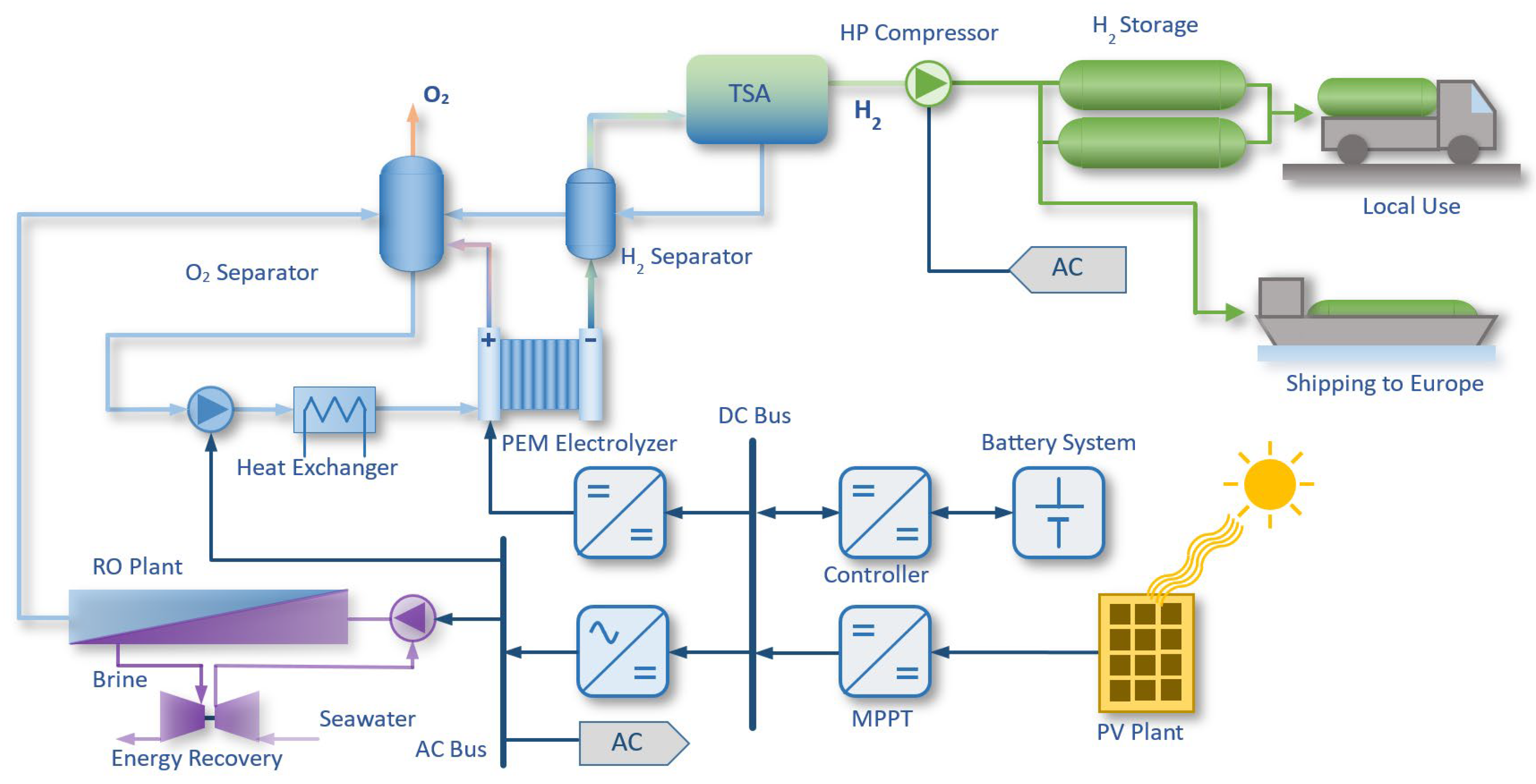
Figure 2.
RO operation with 45% fixed recovery rate.
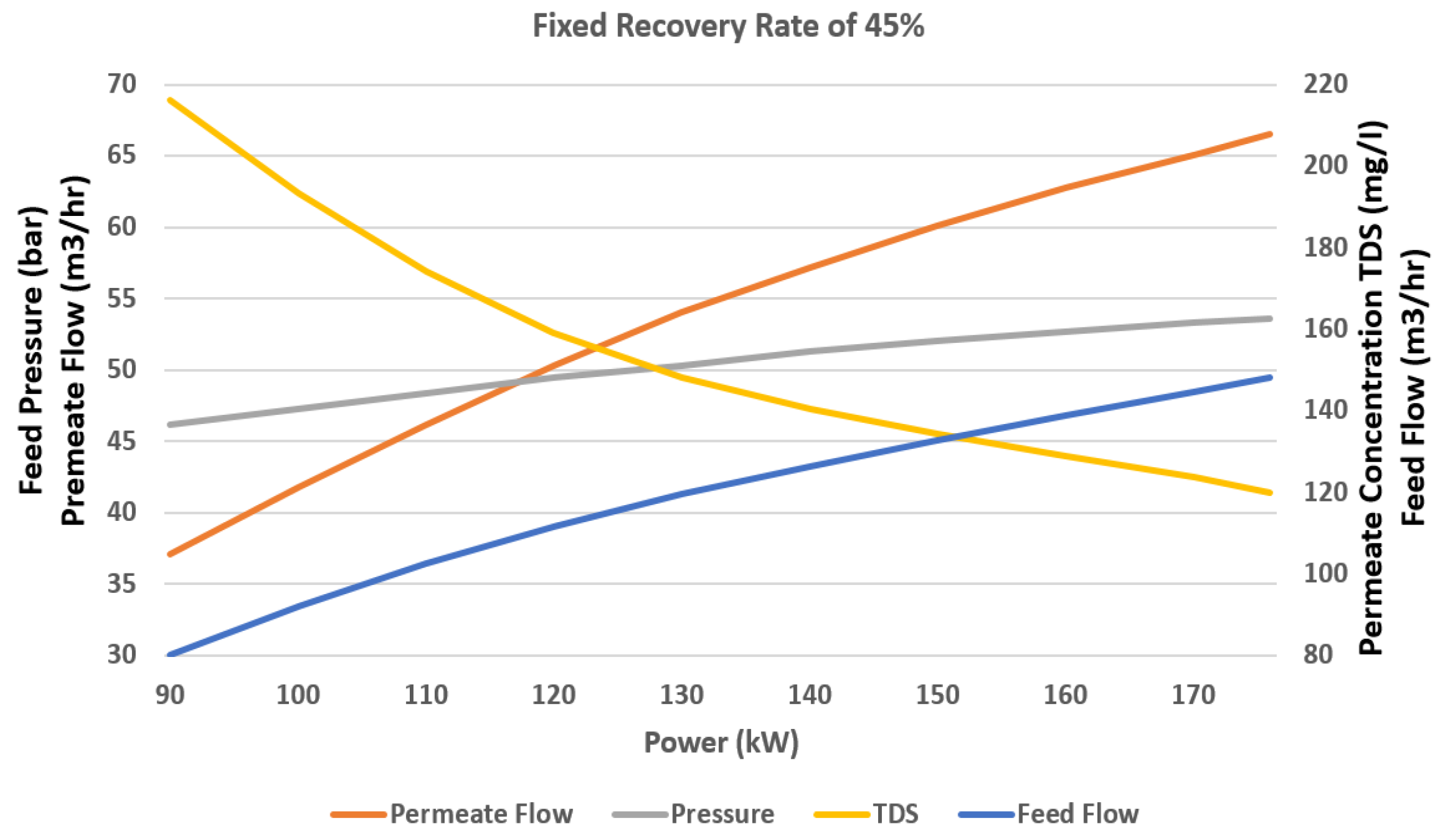
Figure 3.
Type IV green hydrogen storage tank.
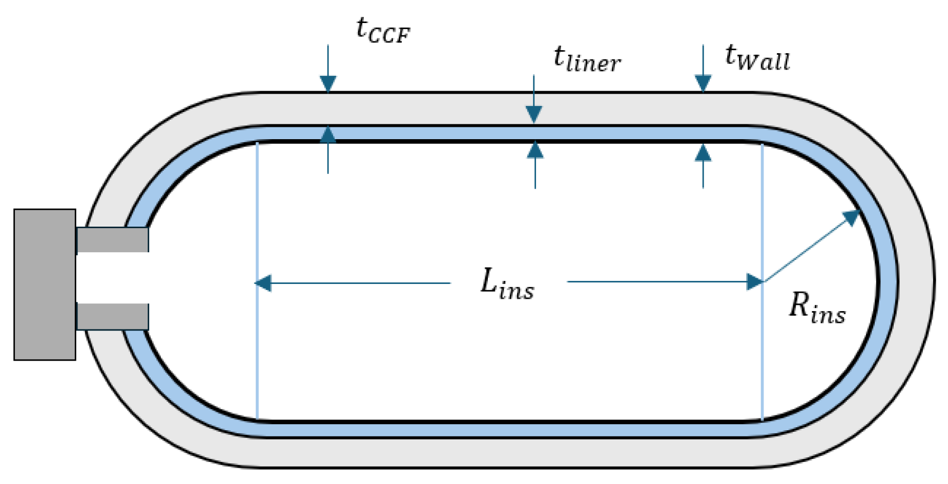
Figure 4.
Variation of tank mass and tank material specific cost at different pressures.
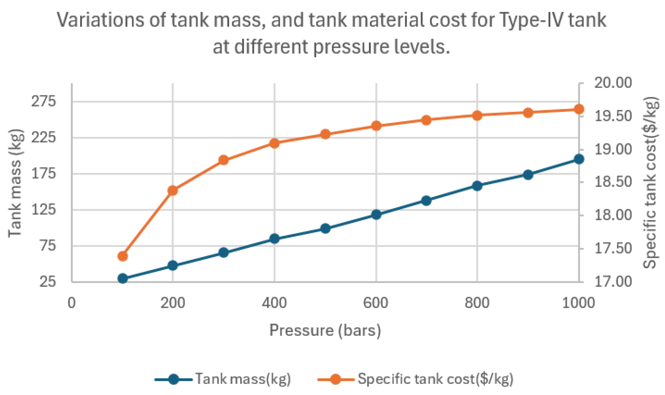
Figure 5.
Ordinal optimization flow chart.
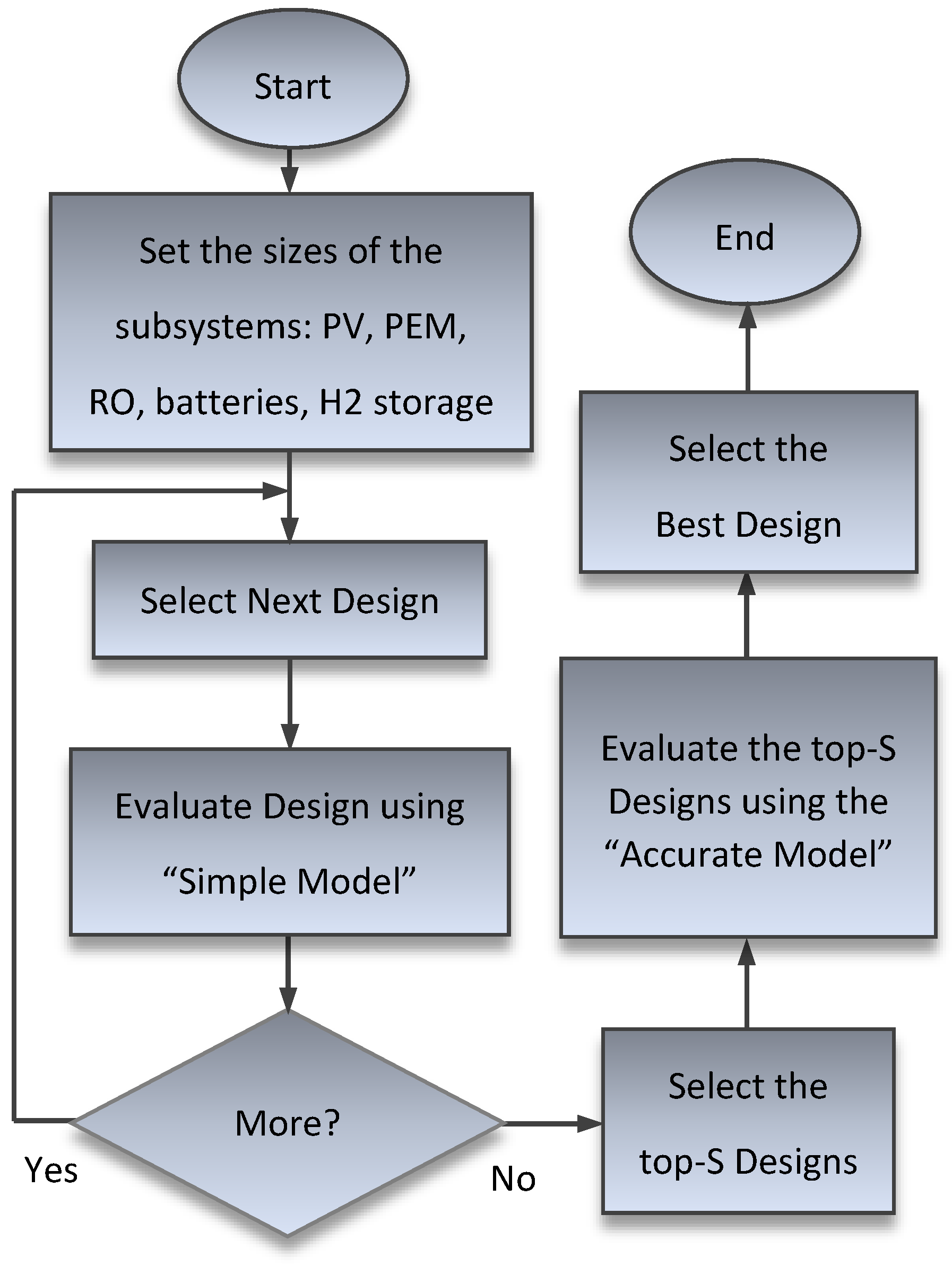
Figure 6.
Energy management System logic.
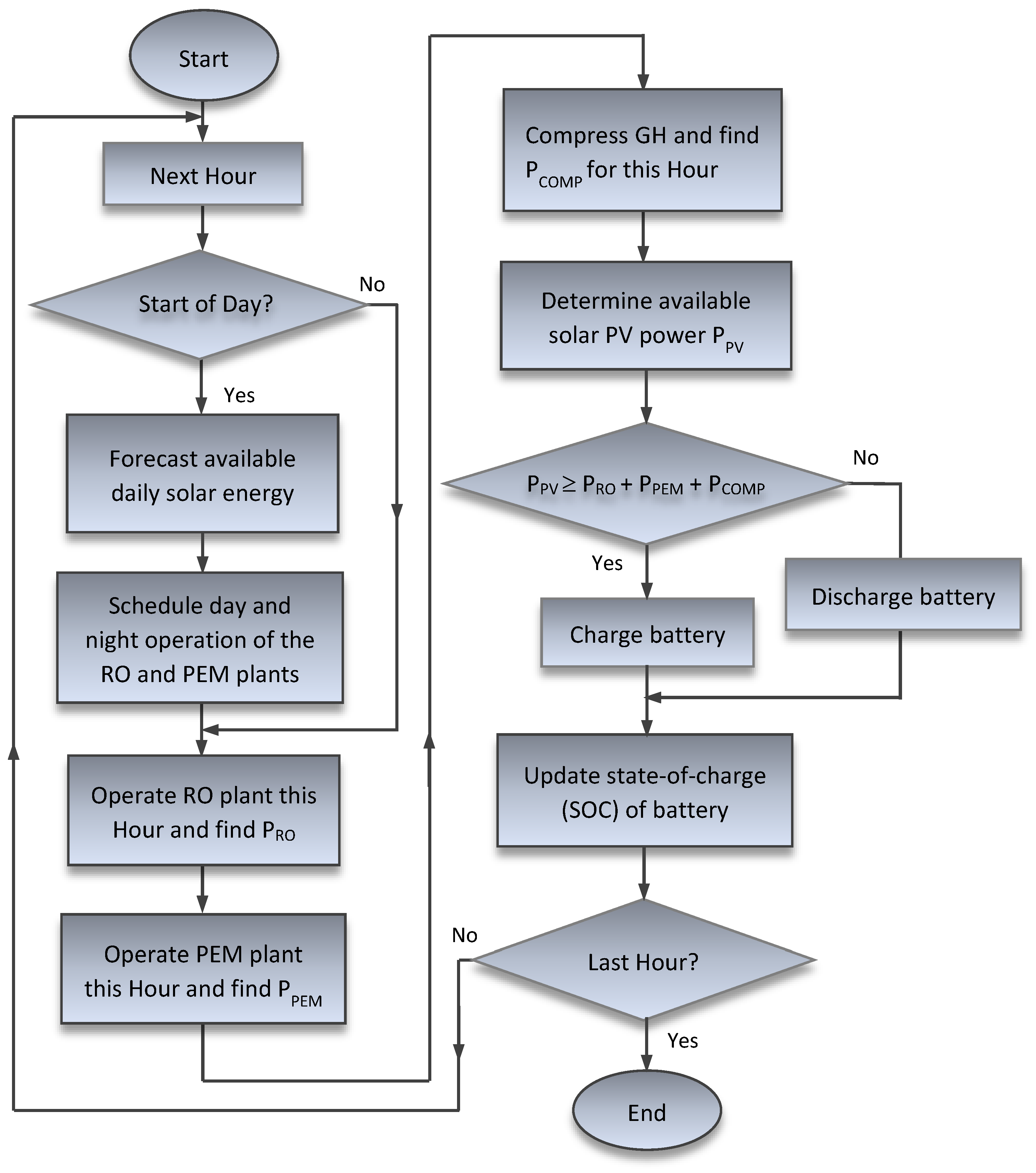
Figure 7.
Ordered performance curve (OPC) – local use scenario.
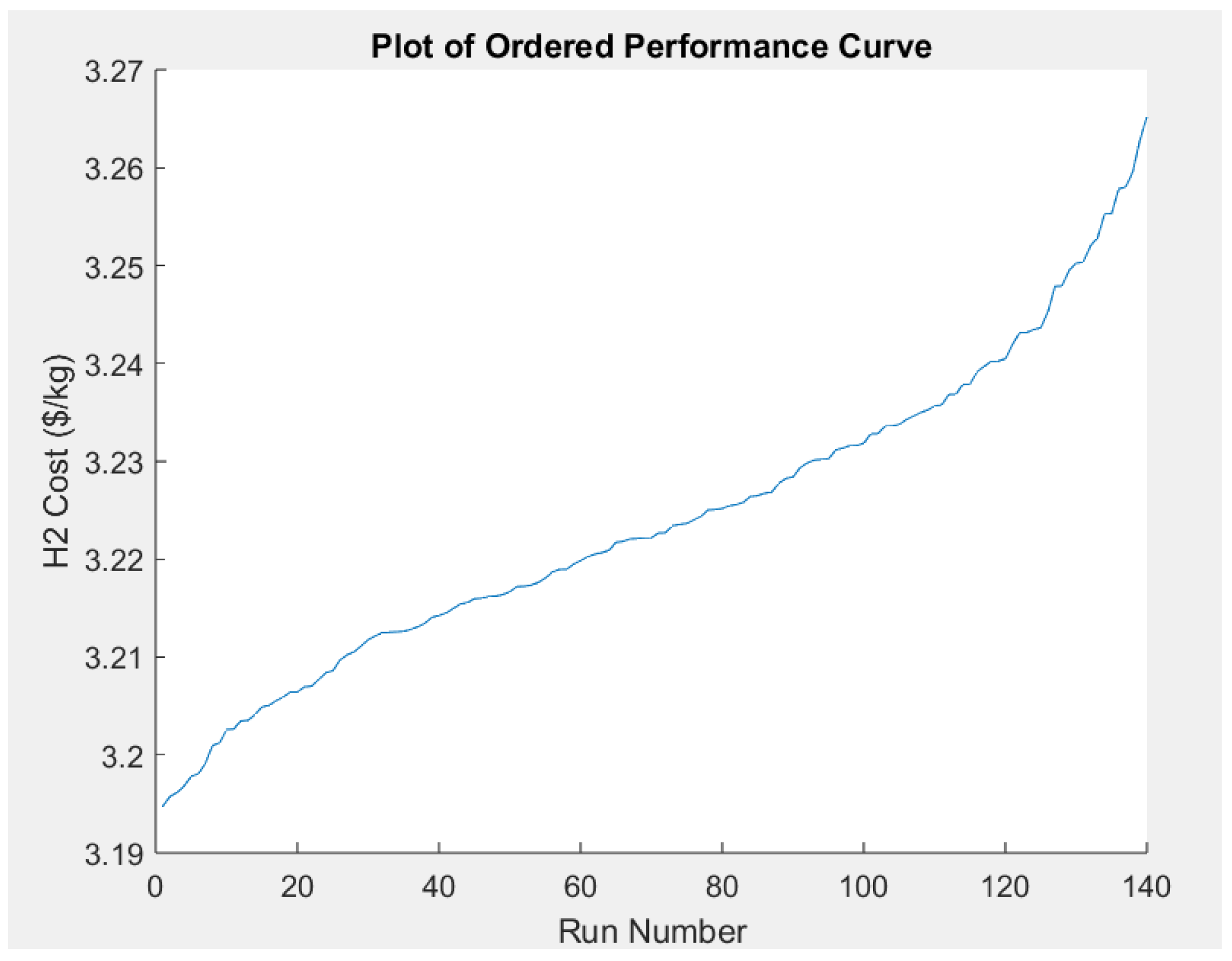
Figure 8.
PV energy production over one year.
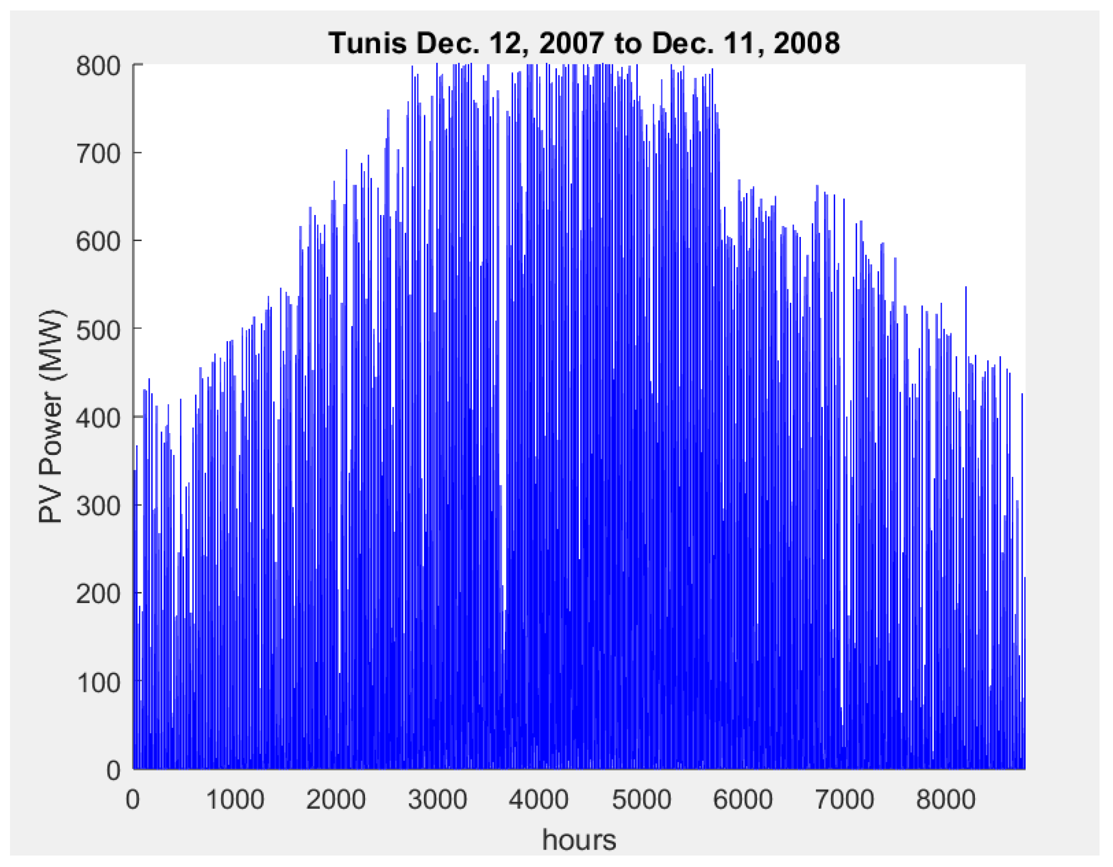
Figure 9.
GH production over the year.
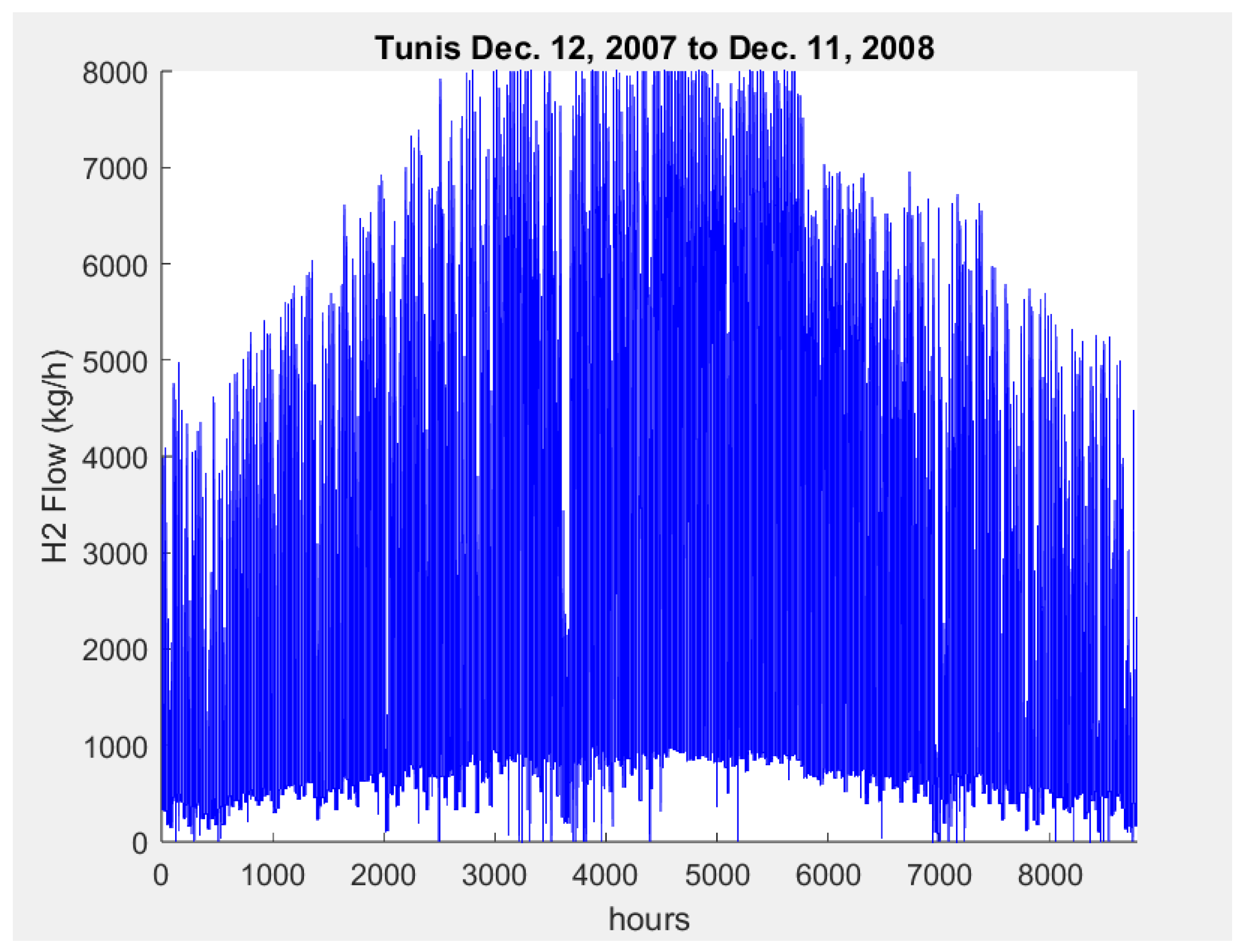
Figure 10.
Filling of ships of Tunis-Genoa for hours 3000 to 5500.
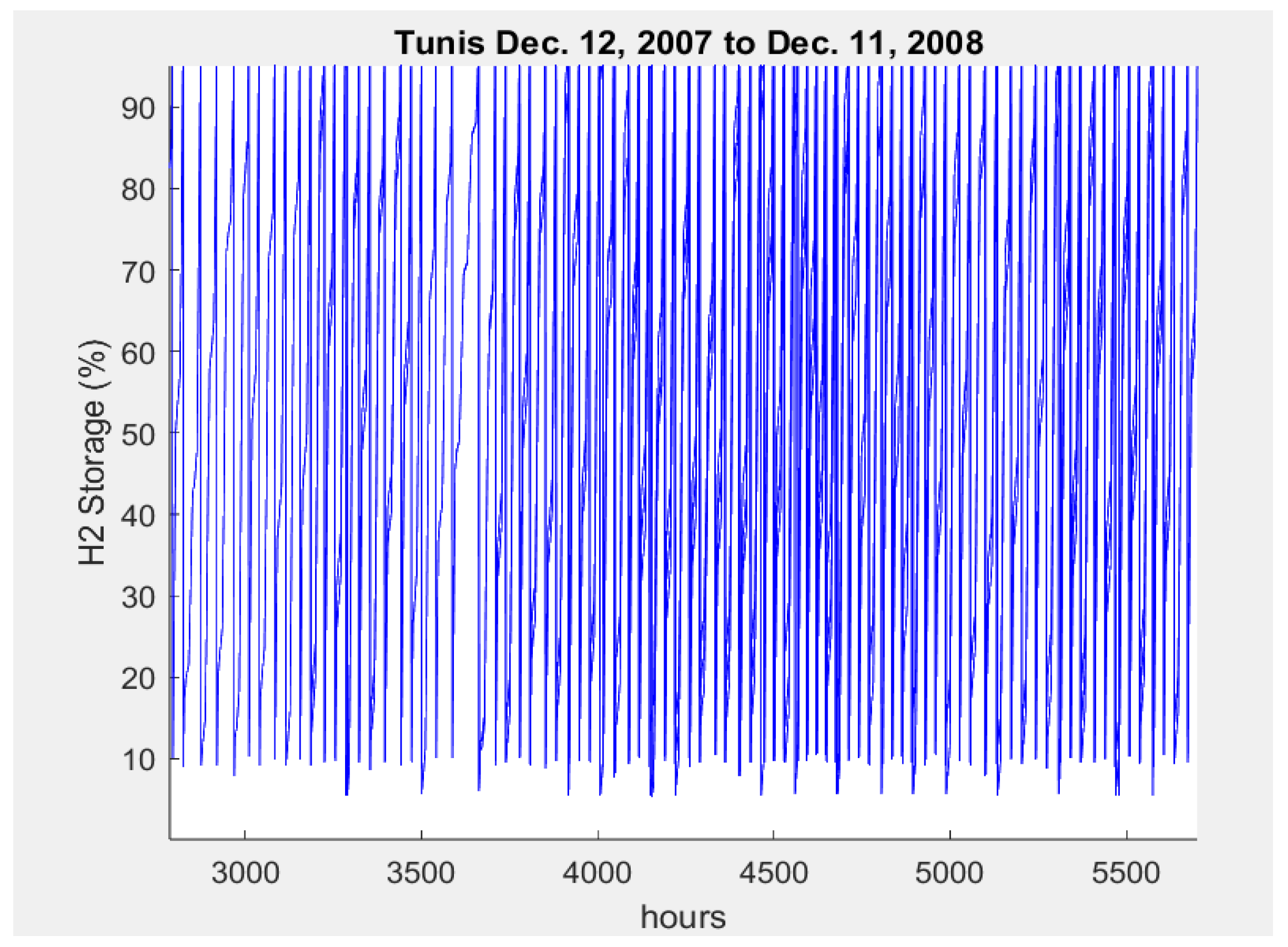

Table 1.
Cost data of primary components.
| PV system | $0.466/ W [30] |
| PEM electrolyzer | $18,300/ (kg/h H2) [31] |
| H2 compression | $450/ (kg/h) at 100 bars [32] |
| Sodium ion battery | $44/ kWh [33] |
| Hydrogen ship hull | $2.7/kg of Ship DWT [18] |
| Fuel cell | $1500/ kW [34] |
| Type IV storage tank @500 bars | $ 243.4/ kg [26] |
Table 2.
Subsystem design sizes.
| Name of Subsystem | Design Values |
| PV Size (MW) | 840, 870, 900, 930 |
| PEM Size (tons/day) | 102, 105, 107, 110 |
| Battery Size (MWh) | 1728, 1782, 1836 |
| RO Size (m3/h) | 56.25, 75.0, 93.75 |
| H2 Pressure (bars) | 300, 500 |
| H2 Storage (days) | 5, 7, 10, 14 |
Table 3.
The top twenty of the “good enough” designs – local use.
| No. | PV MW | BT MWh |
PEM t/day |
RO m3/h |
H2 Store tons |
H2 Prod. t/day |
H2 Cost $/kg |
|---|---|---|---|---|---|---|---|
| 1 | 900 | 1836 | 102 | 56.25 | 267 | 61.9 | 3.19 |
| 2 | 930 | 1836 | 102 | 56.25 | 267 | 63.1 | 3.20 |
| … | … | … | … | … | … | … | … |
| 5 | 930 | 1782 | 102 | 56.25 | 267 | 62.7 | 3.20 |
| 6 | 870 | 1728 | 102 | 56.25 | 267 | 59.8 | 3.20 |
| 7 | 900 | 1728 | 105 | 56.25 | 267 | 61.1 | 3.20 |
| 8 | 930 | 1728 | 102 | 56.25 | 267 | 62.3 | 3.20 |
| … | … | … | … | … | … | … | … |
| 16 | 930 | 1782 | 105 | 56.25 | 273 | 62.9 | 3.21 |
| … | … | … | … | … | … | … | … |
| 20 | 870 | 1836 | 105 | 56.25 | 273 | 60.7 | 3.21 |
Table 4.
The top three designs – local use.
| Run Number | 1 | 2 | 3 |
| PV Size (MW) | 930 | 930 | 930 |
| Battery Size (MWh) | 1728 | 1782 | 1782 |
| PEM Size (t/day) | 102 | 102 | 105 |
| RO Size (m3/h) | 56 | 56 | 56 |
| Net H2 Storage (tons) | 267 | 267 | 273 |
| Storage Pressure (bars) | 500 | 500 | 500 |
| PV Energy (GWh) | 1434.9 | 1434.9 | 1434.9 |
| PEM Energy (GWh) | 1,357.0 | 1,354.8 | 1,360.8 |
| Compression (GWh) | 59.9 | 60.0 | 60.0 |
| RO Energy (GWh) | 1.019 | 1.020 | 1.020 |
| Excess Energy (%) | 0.83 | 0.57 | 0.70 |
| Total Investment (M$) | 660.1 | 662.4 | 665.8 |
| Capex + Opex (M$/ year) | 72.0 | 72.4 | 72.8 |
| H2 Production (t/day) | 66.5 | 66.7 | 67.0 |
| H2 Production (t/year) | 24,280 | 24,344 | 24,449 |
| H2 Cost ($/kg) | 2.966 | 2.974 | 2.976 |
Table 5.
Subsystem Design Sizes.
| Name of Subsystems | Design Values |
| PV Size (MW) | 930, 900, 870, 840 |
| PEM Size (tons/day) | 102, 105, 107, 110 |
| Battery Size (MWh) | 1728, 1782, 1836 |
| RO Size (m3/h) | 56.25, 75.00, 93.75 |
| H2 Pressure (bars) | 300, 500 |
| Ship (Length (m), Number) Tunis - Genoa |
(130, 3), (130, 4), (120, 3), (120, 4) |
| Ship (Length (m), Number) Tunis - Hamburg |
(130, 4), (130, 5), (130, 6), (130, 7) |
Table 6.
The Top 20 Shipping Designs – Tunis to Genoa.
| Run | PV MW | BT MWh |
PEM t/day |
RO m3/h |
H2 Stor. tons |
H2 Prod. t/day |
H2 Cost $/kg |
|---|---|---|---|---|---|---|---|
| 1 | 900 | 1836 | 110 | 56.25 | 111 | 66.0 | 3.97 |
| 2 | 900 | 1836 | 107 | 56.25 | 111 | 65.7 | 3.98 |
| … | … | … | … | … | … | … | … |
| 8 | 900 | 1782 | 102 | 56.25 | 111 | 65.0 | 3.98 |
| 9 | 900 | 1728 | 110 | 56.25 | 111 | 65.6 | 3.95 |
| 10 | 900 | 1836 | 110 | 93.75 | 111 | 66.0 | 3.99 |
| 11 | 900 | 1728 | 107 | 56.25 | 111 | 65.4 | 3.95 |
| … | … | … | … | … | … | … | … |
| 17 | 870 | 1836 | 107 | 56.25 | 111 | 64.0 | 3.97 |
| … | … | … | … | … | … | … | … |
| 19 | 870 | 1782 | 110 | 56.25 | 111 | 64.2 | 3.95 |
| 20 | 900 | 1782 | 110 | 93.75 | 111 | 65.8 | 3.98 |
Table 7.
Top three designs of Tunis-Genoa shipping scenario.
| Run Number | 1 | 2 | 3 |
| PV size (MW) | 900 | 900 | 900 |
| Battery size (MWh) | 1728 | 1728 | 1728 |
| PEM size (t/day) | 110 | 107 | 105 |
| RO size (m3/h) | 56.25 | 56.25 | 56.25 |
| H2 (tons/ ship) | 111 | 111 | 111 |
| Storage pressure (bars) | 500 | 500 | 500 |
| Ship Length (m) | 120 | 120 | 120 |
| Number of Ships | 3 | 3 | 3 |
| Trips per Year | 220 | 220 | 220 |
| PV energy (GWh) | 1,388.6 | 1,388.6 | 1,388.6 |
| PEM Energy (GWh) | 1,310.0 | 1,311.8 | 1,313.6 |
| Compression (GWh) | 60.6 | 60.5 | 60.4 |
| RO Energy (GWh) | 0.998 | 0.997 | 0.996 |
| Excess energy (%) | 0.88 | 0.76 | 0.64 |
| Total investment (M$) | 793.3 | 791.5 | 789.6 |
| Capex + Opex (M$/year) | 93.5 | 92.4 | 92.3 |
| H2 production (t/day) | 65.6 | 65.4 | 65.1 |
| H2 Delivery (t/year) | 23,686 | 23,599 | 23,505 |
| H2 cost ($/kg) | 3.909 | 3.915 | 3.923 |
Table 8.
The First Twenty Designs: Shipping Tunis – Hamburg.
| Run | PV MW | BT MWh |
PEM t/day |
RO m3/h |
H2 Stor. tons |
H2 Prod. t/day |
H2 Cost $/kg |
|---|---|---|---|---|---|---|---|
| 1 | 870 | 1836 | 110 | 56.25 | 141 | 61.1 | 6.47 |
| 2 | 870 | 1836 | 107 | 56.25 | 141 | 60.9 | 6.48 |
| … | … | … | … | … | … | … | … |
| 5 | 870 | 1836 | 105 | 56.25 | 141 | 60.7 | 6.50 |
| 6 | 870 | 1782 | 107 | 56.25 | 141 | 60.5 | 6.50 |
| 7 | 870 | 1836 | 107 | 93.75 | 141 | 60.9 | 6.51 |
| … | … | … | … | … | … | … | … |
| 17 | 870 | 1728 | 107 | 56.25 | 141 | 60.2 | 6.52 |
| 18 | 870 | 1782 | 105 | 93.75 | 141 | 60.4 | 6.53 |
| … | … | … | … | … | … | … | … |
| 20 | 870 | 1728 | 105 | 56.25 | 141 | 60.0 | 6.53 |
Table 9.
The Top Three Designs: Tunis – Hamburg.
| Run Number | 1 | 2 | 3 |
| PV size (MW) | 870 | 870 | 870 |
| Battery size (MWh) | 1728 | 1782 | 1728 |
| PEM size (t/day) | 107 | 107 | 105 |
| RO size (m3/h) | 56 | 56 | 56 |
| H2 (tons/ ship) | 141 | 141 | 141 |
| Storage pressure (bars) | 500 | 500 | 500 |
| Ship Length (m) | 130 | 130 | 130 |
| Number of Ships | 6 | 6 | 6 |
| Trips per Year | 169 | 169 | 169 |
| PV energy (GWh) | 1342.3 | 1342.3 | 1342.3 |
| PEM Energy (GWh) | 1272.1 | 1274.7 | 1273.5 |
| Compression (GWh) | 58.1 | 58.2 | 58.0 |
| RO Energy (GWh) | 0.974 | 0.974 | 0.973 |
| Excess energy (%) | 0.50 | 0.31 | 0.40 |
| Total investment (M$) | 1075.7 | 1078.1 | 1073.9 |
| Capex + Opex (M$/year) | 148.0 | 148.3 | 147.8 |
| H2 Production (t/day) | 63.8 | 63.9 | 63.5 |
| H2 Delivery (t/year) | 23,114 | 23,158 | 23,019 |
| H2 cost ($/kg) | 6.401 | 6.405 | 6.418 |
Table 10.
Comparison Between this Study and Previous Studies.
| Subsystem | Specific Energy | Earlier Studies |
| PEM (kWh/kg H2) |
55.2 | 54.6 [36] |
| 56.8 [6] | ||
| Reverse Osmosis (kWh/m3) |
4.56 | 3.7 [2] |
| 3.5 – 6 [38,39] | ||
| Compression (kWh/kg H2) |
2.49 | 2.2 – 4 [35,37] |
Table 11.
Times in Seconds to Find the Optimum Design.
| Case Study | Exhaustive Search | OO Search | OO Search Design |
| Local Use | 247 | 14.4 | Optimal |
| Tunis – Genoa | 259 | 14.3 | Second Best |
| Tunis – Hamburg | 259 | 14.6 | Optimal |
Disclaimer/Publisher’s Note: The statements, opinions and data contained in all publications are solely those of the individual author(s) and contributor(s) and not of MDPI and/or the editor(s). MDPI and/or the editor(s) disclaim responsibility for any injury to people or property resulting from any ideas, methods, instructions or products referred to in the content. |
© 2026 by the authors. Licensee MDPI, Basel, Switzerland. This article is an open access article distributed under the terms and conditions of the Creative Commons Attribution (CC BY) license (http://creativecommons.org/licenses/by/4.0/).
Copyright: This open access article is published under a Creative Commons CC BY 4.0 license, which permit the free download, distribution, and reuse, provided that the author and preprint are cited in any reuse.


