

Submitted:
07 July 2026
Posted:
08 July 2026
You are already at the latest version
Abstract
Constitutive models for clays have historically treated yield geometry, plastic-flow direction, and compression as separate problems, with little regard for their interaction. This paper tests that assumption by coupling Chatwong et al.’s verified teardrop yield surface with a stress-fractional flow rule and an AJOP-derived hardening modulus in a 2×2×2 factorial design, integrated incrementally along a shear-strain-controlled path. Using real Boston Blue Clay and London Clay parameters, no single main effect or interaction dominates: the flow main effect is consistently largest, the flow×compression interaction is comparably large wherever defined, and compression’s role grows substantially with overconsolidation ratio. Two structural singularities are identified: a phase-transformation point in the teardrop surface’s non-associated flow rule, absent from the fractional rule, and a hardening singularity in the AJOP-based modulus, whose tangent falls to the swelling index at a finite, soil-dependent preconsolidation stress, bounding the evaluable overconsolidation range of the compression-related interactions; a proportional-κ variant removes this singularity by construction while preserving the factorial ranking, identifying it as a property of the constant-κ embedding, not of AJOP itself. Under an approximate undrained path the geometry×flow interaction carries over unchanged, while compression’s role is suppressed several-fold. Chatwong et al.’s validation of the borrowed surface against real undrained triaxial data for all four calibrated soils is reproduced; the incremental framework built on it is not yet validated to the same standard.
Keywords:
fractional plasticity
; stress-fractional flow rule
; teardrop yield surface
; nonlinear compression
; AJOP
; overconsolidated clay
; component-interaction hypothesis
; critical state soil mechanics
1. Introduction
A constitutive model is often built the way an engineer builds a machine: design each part to perform well on its own testbench, then assemble the parts and expect the whole to behave as well as its best-tested component. Applied to clay plasticity, this assumption says that the yield surface, the flow rule, and the compression law can each be validated separately — against triaxial strength data, against dilatancy data, against oedometer data — and then combined without asking whether the combination itself changes anything. Fifty years of constitutive-modelling research has largely proceeded on this assumption, refining yield geometry, plastic flow, and compression laws as three separate problems, each owned by a different research community with its own benchmark tests [1,2]. The assumption is testable, but to the authors’ knowledge it has never actually been tested for these three components together. If a fractional-order operator acts directly on the yield surface to generate flow direction, and the hardening law that scales that operator is itself derived from the same state variable that also fixes the yield-surface size, then geometry, flow, and compression may not be separable parts at all — and fifty years of testing them one at a time would simply never have revealed it.
The three research lines were indeed developed largely in isolation. Yield geometry was refined against strength and dry-side data: Hvorslev-type and composite extensions [3,4,5,6,7,8,9] and later generalized, smooth surfaces [10] and continuous teardrop-type surfaces [11] were each validated against peak-strength envelopes, essentially independently of how flow direction or hardening was modelled. Constitutive evolution was refined against a different benchmark again — bounding-surface and subloading-surface formulations [12,13,14,15,16,17] were validated against stiffness-degradation and cyclic data, with no particular yield geometry or flow operator presumed.
Plastic flow was refined against a third, largely independent benchmark: stress-dilatancy data. Associated flow was rejected because it cannot match observed dilatancy in dense sands and overconsolidated clays [18,19,20]; classical non-associated models such as MIT-E3 and MIT-S1 [21,22,23], and more recently stress-fractional flow operators [24,25,26,27,28], were both validated primarily against dilatancy and stress-ratio data, largely independently of which yield surface or hardening law happened to be attached to them. The work of Sumelka [24] initiated the use of fractional flow rules to generate non-normality; Sun and co-workers extended this to granular soils, bounding-surface frameworks, true triaxial loading, cyclic behavior, interfaces, and overconsolidated clays; and Qu, Sun and Sumelka [27] synthesized the role of stress length scale and fractional flow in stress-fractional plasticity — an extensive literature, but one that has advanced the flow operator on its own terms.
Compression was refined against a fourth benchmark, oedometer data, and reveals the same pattern most starkly. Classical critical-state models assume the e–ln p′ relationship is linear, an assumption most realistic only for normally consolidated clays over a limited stress range [2]; work on unsaturated and highly compacted clays later showed that a single linear index cannot represent behavior consistently from low to very high stress [29]. Kaewhanam and Chaimoon (2023) found, in the context of their simplified silty sand (SSS) model, that linear functions in e–ln p are accurate at high stress but inaccurate at low stress, while curved (power-law) functions show the opposite tendency, and introduced a closed-form equation joining the two within a single expression [30]; Phonchamni et al. subsequently adapted this joining construction to the virgin compression of clays as the revised Arc Joint via Optimum Parameters (AJOP) equation, reducing settlement-prediction error by up to 85% relative to a linear index and by 10–15% relative to a purely curved index [31]. AJOP is, mechanically, the same kind of continuity fix that motivated the teardrop yield surface and the fractional flow operator — yet it has so far been used only as a stand-alone settlement equation, never embedded as the hardening modulus inside a yield-surface-and-flow-rule framework.
This is where the machine-building assumption becomes questionable rather than merely convenient. Fractional plasticity does not replace the yield surface; it replaces the operator acting on the yield surface, so its output depends on the geometry on which it acts. The hardening rate is a third ingredient that cannot be waved away as background: it scales the plastic multiplier dλ appearing in every flow-rule equation, and it governs how quickly the preconsolidation size — and hence the point on the yield surface at which the fractional operator is evaluated — evolves along a stress path. If the compression law is itself nonlinear and stress-dependent, as AJOP asserts, then two independently state-dependent quantities, the fractional order and the hardening modulus , are driven by the same underlying state along the same stress path. There is therefore a concrete mechanical channel through which geometry, flow, and compression could interact rather than simply add up — and no existing study has tested this three-way interaction directly, because no existing study needed to: each component had already been declared successful on its own testbench.
Qu, Sun, and Sumelka’s own review [27] hints at half of this picture without completing it: it emphasizes that fractional plasticity is an efficient alternative for state-dependent nonassociativity, while separately noting the importance of improved yield-surface architecture, including reduced dry-side elastic-region surfaces for geomaterials. That observation motivates pairing geometry with flow; it says nothing about compression, which is why the present study treats compression as a third, independently motivated component rather than an afterthought bolted on for symmetry.
The objectives of this paper are therefore threefold. First, it formulates a component-based constitutive design in which yield geometry, plastic flow, and the compression/hardening law are explicitly identified as the three modified components, while constitutive evolution (mapping rules) is intentionally left unmodified so the three-way interaction can be isolated. Second, it embeds the revised AJOP compression law [31] as a nonlinear, stress-dependent hardening modulus , replacing the constant compression index λ used in conventional critical-state hardening, and couples it to a continuous teardrop yield surface [11] and a state-dependent fractional stress-gradient flow rule. Third, it proposes a 2×2×2 factorial numerical assessment that separates the individual, pairwise, and three-way interaction effects of geometry, flow, and compression, so that the assumption of separability — not just the interaction hypothesis — can be tested rather than taken for granted.
2. Materials and Methods
This section formulates the constitutive framework analytically; no laboratory testing was performed for this study. Section 2.1, Section 2.2, Section 2.3, Section 2.4, Section 2.5, Section 2.6, Section 2.7, Section 2.8 and Section 2.9 present the model formulation, and Section 2.10 presents the numerical-assessment design used to test the components’ interaction (Section 3).
2.1. Component-Based Design Concept
The proposed framework decomposes a constitutive model into interacting components. In the present study, three components are modified — yield geometry, plastic flow, and the compression/hardening law — while constitutive evolution (bounding-surface or subloading-surface mapping rules) is intentionally left in its simplest conventional form, since no mapping rule is used in either the baseline or the proposed model. This keeps the comparison in Section 3 attributable to the three components under test rather than to a fourth, unmodified mechanism.
2.2. Continuous Teardrop Yield Geometry
Let p′ be the mean effective stress, q the deviatoric stress, the size parameter of the yield surface, and M the critical-state stress ratio. The normalized mean stress and normalized deviatoric stress are defined as
Following the continuous teardrop concept, the working yield function used in this study is
where Ψ controls the skewness/curvature of the teardrop geometry and Ω adjusts the strength scale. This is the closed-form yield function of Chatwong et al. [11] (their Equation 2, with , rearranged into the form above and verified directly against the published source rather than reconstructed from memory). Ψ and Ω are taken from Chatwong et al. [11]’s own calibration for the specific clay used (their Table 1; Section 3.3). The yield function is therefore written generally as
2.3. Classical and Non-Associated Flow
In associated plasticity, plastic strain increments are normal to the yield surface,
where dλ is the plastic multiplier and is the effective stress tensor. Classical non-associated plasticity instead introduces a separate plastic potential g,
which is effective but separates stress admissibility from plastic-flow direction.
Chatwong et al. [11] themselves adopt exactly this classical non-associated route: their teardrop yield surface f is paired with a separate, simpler plastic potential g (of Original-Cam-Clay form, , giving a closed-form, purely linear dilatancy relation that is independent of the teardrop shape parameters and . This is a legitimate and economical choice, but it means the flow direction in their model does not depend on the yield-surface shape at all — the two components are decoupled by construction. The present study deliberately does not follow that route. Section 2.4 instead applies the fractional operator directly to f, so that flow direction is generated from the same shape parameters that define the yield surface, without introducing a second, independent potential function. This is not a criticism of [11]’s choice; it is a different design decision precisely because it is the one whose consequences (Section 2.8) this paper sets out to test.
This is not a purely local design choice. Xu, Shen and Sun [32] independently develop a fractional-plasticity model for a soil–structure interface that, like the present study, combines a state-dependent fractional order with a state-dependent hardening modulus and explicitly avoids introducing an additional plastic potential; their model, however, is built on a fixed Cam-clay-type loading surface rather than a curvature-controlled yield geometry such as the teardrop surface, so it does not test whether the fractional operator’s output changes when the underlying geometry itself is varied — precisely the question Section 2.8 and Section 3 address here.
2.4. Stress-Fractional Flow Operator and Stress Length Scale
Stress-fractional plasticity modifies the flow operator instead of introducing an independent plastic potential:
where ᶠ∇^α_ denotes the fractional stress-gradient operator and α is the fractional order. In principal effective stress space,
A stress length scale (SLS) is required to make the fractional derivative well defined. A Caputo-type stress-fractional derivative is adopted provisionally,
where is the stress length scale (SLS) in the σ′_i direction. Qu, Sun and Sumelka [27] identify three conventions for defining the SLS in the fractional plasticity literature: a past-stress (“long memory”) convention, in which l_i spans from the initial stress state to the current state; a future-reference (“critical-state”) convention, in which spans from the current state to a future critical state; and a combined convention using both. Sun and co-workers’ own models [25,26,28] adopt the critical-state convention, and this study follows them: is taken as the distance, in the relevant normalized stress coordinate, from the current state to the critical state line . For both the classical and teardrop geometries used here, this critical-state point coincides exactly with the phase-transformation point identified in Section 3.4 (=0.5 for the classical ellipse, ≈0.341 for the teardrop surface with the real =0.93 used in Section 3, both obtained by setting in the corresponding classical yield curve and the teardrop yield curve of Equation (2), respectively) — so is fully determined by the state variables already in the model, with no additional free parameter. The numerical results in Section 3 approximate this state-dependent SLS with a fixed small step h and a finite number of terms N (Section 3.1), rather than integrating the Grünwald–Letnikov sum out to the exact distance at every step. As implemented, the approximation departs from the critical-state convention in two respects, not one: the window has a fixed length N·h rather than the state-dependent length , and it extends in the past-stress direction (below the current ) rather than toward the critical state, so the scheme realises a fixed-length window of the past-stress type while the critical-state convention above is adopted conceptually. Replacing it with the exact state-dependent bound is a specific, well-defined numerical task for future work rather than an open conceptual question (Section 2.9). The associated flow rule is recovered as the limiting case
2.5. State-Dependent Fractional Order
The fractional order is linked to overconsolidation because the degree of non-associativity generally increases as the soil becomes more overconsolidated. The simplest admissible form is
which gives α(1) = 1 for normally consolidated clay and < 1 for OCR > 1. A bounded exponential form may also be used:
with α(1) = 1 and →αmin as OCR→∞.
2.6. Nonlinear AJOP Compression Law as the Hardening Modulus
Conventional critical-state hardening assumes a constant compression index λ, i.e., a straight virgin compression line in e–ln p′ space. The revised AJOP equation of Phonchamni et al. [31], adapted from Kaewhanam and Chaimoon [30], instead represents the e–log v relationship as
where Γ, , R and θ are the AJOP shape parameters. The subscript on a_c is used deliberately throughout this paper to avoid confusion with the fractional order α used in Section 2.4 and Section 2.5 — the two symbols are unrelated. Because the teardrop-and-fractional-flow formulation above is written in terms of mean effective stress rather than the one-dimensional used in oedometer calibration, is adopted here as a working idealisation; a proper isotropic (or K0-consistent) recalibration of Γ,, R and θ from triaxial or isotropic compression data is left as an open item (Section 2.9).
The instantaneous (tangent) compression modulus is obtained by differentiating Equation (12) with respect to ln . Writing x = log10(p′/R),
This expression provides a useful internal consistency check. As p′→R (x→0), the bracketed term vanishes and → a_c/ln 10; as p′ becomes large (x→∞), the bracketed term tends to 1 and → , a constant asymptotic slope. The tangent modulus therefore rises smoothly from a lower value near the reference stress to a fixed asymptotic value at high stress — which is precisely the “curved segment joined to a linear segment” behaviour that motivated AJOP in the first place [30,31], and gives a first check that Equation (13) has been derived correctly.
The choice to use as the hardening modulus, rather than as a separate post-processing correction, follows from what a hardening modulus is defined to be. In critical-state plasticity, the modulus that appears in the hardening law is, by construction, the tangent slope of whichever compression curve is taken as the model of virgin behaviour — a constant λ is not a physical assumption in its own right, but simply the tangent slope of the linear e–ln p′ model. If AJOP is accepted as a more accurate representation of that same curve across the full stress range [30,31], consistency requires using its tangent, not the tangent of the linear approximation it was built to replace, as the hardening modulus. Equation (13) is therefore not a substitution of convenience; it is the hardening modulus implied by taking AJOP, rather than a straight line, as the compression law, obtained the same way λ itself is obtained from the linear model. The remaining question, addressed numerically in Section 3, is whether this consistent choice produces a response that differs materially from the constant-λ case once it is embedded in a flow rule.
Equation (13) also has a second, physically meaningful limit that is not captured by a constant-λ line. As , i.e., as , the bracketed term in Equation (13) tends to −1, so →0, while Equation (12) gives e→Γ. In other words, Γ acts as an upper bound on void ratio that AJOP approaches asymptotically at very low stress, rather than a value the compression curve passes through and continues beyond. A constant-λ line has no such bound: extrapolated to low stress it predicts an unbounded increase in e, which is not physically possible. This distinction becomes numerically important precisely in the low-stress, far-below-calibration region relevant to shallow soft-clay layers, and is examined quantitatively for three real clays in Section 3.4.
The conventional hardening law,
is therefore replaced by its AJOP-based, stress-dependent counterpart,
in which is re-evaluated at the current at every increment. Unlike the constant-λ case, the hardening modulus is now itself a function of the same stress state that also drives in Equation (11), which is the mechanical basis for the three-way interaction hypothesis introduced in Section 2.8.
2.7. Constitutive Architecture
The complete framework consists of four sequential components:
State →
Continuous yield geometry → Fractional flow → AJOP-based nonlinear hardening
First, the stress state is checked against the continuous teardrop yield surface,
Second, the plastic flow direction is obtained from the fractional stress-gradient operator,
Third, the fractional order is evaluated from the overconsolidation state (in the numerical implementation of Section 3, the initial state, held fixed along each path — Section 3.1),
Finally, the hardening variable evolves according to the AJOP-based nonlinear law derived in Section 2.6,
2.8. Geometry–Flow–Compression Interaction Hypothesis
The central hypothesis of this study is that geometry, flow, and compression are not separable. Since the fractional gradient acts on the yield function (Equations 6 and 7), and since the hardening law now scales the same plastic multiplier dλ that appears in that flow rule while also controlling how fast — and hence the point on the yield surface being evaluated — evolves along a stress path, the three components are hypothesized to interact:
H_G×F×C: the
combined effect of geometry, flow and compression is not simply the sum of
their individual and pairwise effects
This coupling is expected to act through two channels: a direct channel, in which and are simultaneously evaluated at a state that also depends on which yield geometry is used to define ; and an indirect, path-dependent channel, in which a nonlinear hardening rate changes the stress path itself, so that geometry and flow are subsequently evaluated at different states than they would be under conventional hardening. Section 3 is designed to test both channels numerically through a full factorial design.
2.9. Stated Approximations and Open Items
Three approximations should be stated explicitly before the numerical implementation. (i) The numerical results in Section 3 realise the stress-length-scale of Equation (8) as a fixed-length (N·h=0.2 in normalised stress), past-stress-direction, truncated Grünwald–Letnikov window rather than the exact state-dependent critical-state bound (Section 2.4); implementing the exact bound is a specific numerical task rather than an open conceptual question. (ii) The fractional order α is evaluated at the initial overconsolidation state and held fixed along each path (Section 3.1); re-evaluating α from the evolving state at every increment is a well-defined extension left for future work. (iii) The AJOP parameters Γ, , R, θ in Equation (12) were calibrated from one-dimensional oedometer data and have not yet been re-derived for the isotropic p′ used elsewhere in this framework.
2.10. Numerical-Assessment Design
The assessment is designed as a constitutive-component experiment rather than a conventional model-validation exercise: the aim is to determine whether the response produced by combining a stress-fractional flow operator with a nonlinear hardening law depends on the underlying yield geometry, and vice versa. Three factors are varied: yield geometry (classical reference surface or continuous teardrop surface), flow operator (classical integer-order gradient or state-dependent fractional stress-gradient), and hardening/compression law (conventional constant-λ or AJOP-based ). This gives a 2×2×2 = 8-framework comparison.
Let R denote a response quantity of interest (e.g., predicted dilatancy, volumetric strain increment, or settlement error against laboratory/field data). The main effects are
the pairwise interaction indices are
and the three-way interaction index, the standard factorial triple-contrast, is
If is close to zero, the three components act additively even though pairwise interactions may still be present. If is non-zero, geometry, flow and compression jointly determine the response in a way that cannot be recovered from any subset of one- or two-component studies. A full benchmark would evaluate the eight frameworks along several stress paths — normally consolidated drained compression, overconsolidated drained compression, undrained compression, and a one-dimensional oedometer-type path that would exercise the AJOP component against the data type it was originally calibrated on [31] — but the present study implements the overconsolidated drained-shear case at constant mean effective stress as the primary test of the factorial design (Section 3.1), together with a second, deliberately approximate check under undrained conditions (Section 4.3); the remaining paths — normally consolidated drained compression and a proper oedometer-type path — are left as future work (Section 5) rather than attempted here.
3. Results
3.1. Numerical Implementation
The eight configurations of Table 2 were evaluated by incrementally integrating a drained shear path at constant mean effective stress, starting from a specified initial OCR. The shear-strain increment dεₛᵖ is treated as the controlled (independent) loading variable, and each step updates . Two points of convention are worth stating explicitly here, since they determine how the numbers in Section 3.3 and Section 3.4 should be read. First, p′ itself is held fixed throughout a given path; it is that evolves, and only because evolves under the hardening law — the path is therefore driven entirely by plastic hardening/softening at constant mean effective stress, not by an externally imposed change in or in itself. Second, positive corresponds to net contraction and negative to net dilation, consistent with εᵥᵖ>0 meaning compressive volumetric strain throughout this paper (Section 2); and therefore carry the same sign in the update equation above, and p̄ increases when is negative (dilative) and decreases when is positive (contractive) for a fixed . The clamps =0.03 and =0.985 in the update equation are numerical safety bounds only — in the runs reported in Section 3.3 and Section 3.4, every framework is net-dilative from the starting state used here (Section 4.1) and so increases rather than decreases; each framework instead stabilizes at an intermediate asymptote well short of (specifically, its own flow rule’s critical-state point: =0.5 for classical-integer, =0.341 for teardrop-integer, and the wet-side values ≈0.868 and≈0.818 for the classical-fractional and teardrop-fractional combinations respectively — equilibria of the fixed-window Grünwald–Letnikov operator itself rather than of the underlying yield surfaces, Section 2.9 and Section 3.1.1), and none reach either clamp; and are retained as bounds for completeness rather than because it is reached by these particular paths.
where is the flow ratio for the chosen geometry×flow combination (Section 3.1.1) and depending on the compression choice, with p′c updated each step from p̄ at fixed p′. Controlling dεₛᵖ rather than dεᵥᵖ matters because any scheme that divides by is singular wherever passes through zero: for teardrop geometry combined with integer-order (Chatwong et al. [11]’s own g-based) flow, passes through exactly zero at (≈0.341 for the real =0.93 used in Section 3) — a genuine phase-transformation point at which the flow direction is purely deviatoric — and dividing by there is singular. Controlling dεₛᵖ instead of dεᵥᵖ removes this singularity entirely, since =0 simply means zero volumetric increment at that step rather than an undefined ratio; this is not a numerical workaround so much as the physically appropriate choice of independent variable for a strain-controlled shear test, and it is retained as the standard scheme throughout Section 3.
The response quantity is accumulated over a fixed shear-strain budget (εₛᵖ=6, =60,000 for full convergence, Section 3.4), so that all eight frameworks are compared after exactly the same amount of imposed shearing. This is a full incremental integration of the coupled flow rule and hardening law along a stress path, not a single-state evaluation, though it remains a simplified one-dimensional (constant-p′) idealisation rather than a general-stress-path implementation, and elastic strains before first yield are not separately tracked.
The two update equations above also imply an exact structural identity that is used throughout as an internal consistency check. Dividing them gives at every increment, so for the constant-λ configurations the accumulated response has the closed form , where is the equilibrium point at which the configuration’s flow rule satisfies =0; for the AJOP configurations, over the same interval. The flow rule therefore influences only through the location of its equilibrium point (and through whether the strain budget suffices to reach it), while the compression law influences R only through the integrand. The reported endpoints reproduce every entry of Table 4 to four to five significant figures through this identity, and — because the critical-state stress ratio M cancels from it — the results of Section 3.3, Section 3.4 and Section 3.5 are independent of M; all calculations are accordingly performed in the normalised coordinates of Equation (1) with M=1 (Section 3.1.1).
3.1.1. Flow Ratio by Geometry × Flow Combination, with Explicit Sign Derivation
For any yield function written as , associated flow is normal to f: the plastic strain increment is proportional to . The dilatancy ratio is the ratio of the volumetric to the shear component of that normal, , not +g′(̄p); the minus sign is not a convention but a direct consequence of for this form of f. This can be checked against the standard critical-state result for Modified Cam Clay written with M retained explicitly: for , the associated dilatancy ratio is , which in terms of the stress ratio η=q/p′ reduces exactly to — negative (dilative) for η>M (the dry side, low ̄p) and positive (contractive) for η<M (the wet side), matching standard critical-state theory (e.g., Roscoe and Burland). Substituting the normalized form and taking reproduces this result up to the constant factor M — in the normalised coordinates of Equation (1), — confirming the sign: for classical (MCC) geometry with integer-order (associated) flow, . Consistent with this, all D values in this study are reported in these normalised units (M=1); by the closed-form identity of Section 3.1 this leaves every response in Table 4 and Table 5 unchanged. The same sign applies to the fractional-order case: the fractional operator generalizes , so D for classical geometry with fractional flow is the negative of the Grünwald–Letnikov fractional derivative of g(̄p), not its raw (positive) value. For teardrop geometry with fractional flow — the present study’s own proposal — the same reasoning applies to the real teardrop yield function: D is the negative of the Grünwald–Letnikov fractional derivative of , with no separate potential required. For teardrop geometry with integer-order flow, D is instead Chatwong et al.’s [11] own (Section 2.3), since that is the flow rule actually proposed alongside their yield surface, and it is not derived from at all — it is [11]’s own non-associated potential, taken directly from their published formulation and left as published throughout this study.
Although the analytical operator in Equation (8) is written in Caputo-type form, the present numerical implementation evaluates the corresponding fractional gradient using a finite-term Grünwald–Letnikov approximation with step size h=0.005 and N=40 terms, which is commonly used for numerical fractional differentiation and converges to the same operator as the step size shrinks and the number of terms grows. The implications of replacing this approximation with the exact state-dependent integration bound now specified in Equation (8) are discussed in Section 2.9.
3.2. Compression-Law Comparison Using Real AJOP Parameters
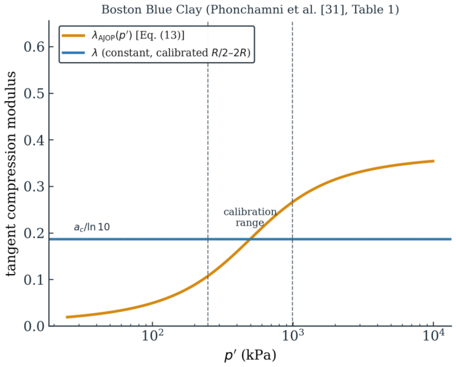
Table 3 uses the AJOP parameters Γ, , R and θ fitted from laboratory oedometer data for three clays by Phonchamni et al. [31] (their Table 1: Boston blue clay, London clay, Bangkok clay). For each soil, a linear compression index was calibrated to match AJOP exactly over R/2–2R, a typical oedometer test range straddling the reference stress — the same procedure a real laboratory calibration would follow. is reported both at p′=R (Equation 13 at x=0) and at its high-stress asymptote (Section 2.6).
For all three soils, calibrated over R/2–2R equals evaluated at exactly (Table 3), a consequence of the symmetry of AJOP’s √ term about x=0: the secant of an even function taken symmetrically about its own center exactly recovers the function’s slope at that center. A linear index fit over a realistic test range therefore does not approximate AJOP’s high-stress asymptotic slope, which is twice as large (Table 3); it reproduces AJOP’s local tangent modulus at the reference stress R exactly, and diverges from AJOP on both sides of R. Extrapolated below the calibration range, the constant-λ line over-predicts the local compressibility relative to AJOP, and does so increasingly as p′ falls further below R, because (per the Γ-bound discussed in Section 2.6) →0 as , while stays constant. This behaviour is qualitatively consistent with the settlement-error asymmetry reported by Phonchamni et al. [31] (larger linear-index error at shallow, lower-stress depths than at deep, higher-stress depths), although the present comparison is illustrative of the mechanism and is not a reproduction of their reported error magnitudes.
Of these three soils, Boston Blue Clay is used as the primary case for the factorial evaluation in Section 3.3 and Section 3.4, in preference to the other two, because it is also one of the clays for which Chatwong et al. [11] independently calibrated and validated the teardrop yield-surface parameters and (their Table 1). Using this soil therefore lets every parameter entering Section 3.3—the yield-surface shape, the flow rule’s implicit non-associated relation, and the compression law—be drawn from experimentally-calibrated sources rather than assumed.
As a basic sanity check on the AJOP parameters themselves, for Boston Blue Clay (0.430, Table 3) is itself a conventional compression index Cc in the e–log₁₀p′ sense used elsewhere in the literature, since AJOP is formulated directly in log₁₀(p′/R) terms (Section 2.6); this is a separate quantity from the ln(p′)-based λ_LF reported in Table 3, which differs from Cc by a factor of ln(10). Reported Cc values for Boston Blue Clay in the literature are commonly of the order of 0.3–0.5; the value used here falls within that range rather than outside it, which is a minimal but real check that the AJOP fit is not producing an unrealistic compression index for this specific, well-studied clay, even though it does not by itself validate the incremental framework built on top of it in Section 3.3 and Section 3.4.
Figure 1.
AJOP tangent compression modulus (Equation 13) compared with a constant linear index λ calibrated over the typical oedometer test range R/2–2R, using the real Boston Blue Clay parameters of Table 3. rises smoothly from near the reference stress R to its high-stress asymptote 2a_c/ln10, whereas the constant-λ line stays flat across the whole stress range.
Figure 1.
AJOP tangent compression modulus (Equation 13) compared with a constant linear index λ calibrated over the typical oedometer test range R/2–2R, using the real Boston Blue Clay parameters of Table 3. rises smoothly from near the reference stress R to its high-stress asymptote 2a_c/ln10, whereas the constant-λ line stays flat across the whole stress range.
3.3. Factorial Results (F0–F7) for Boston Blue Clay
The 2×2×2 factorial design of Table 2 was evaluated using the real Boston Blue Clay AJOP parameters from Table 3 and the real teardrop yield-surface parameters of Chatwong et al. [11] (their Table 1: =1.4, =0.93). The conventional (constant-λ) branch uses λ==0.187, the R/2–2R secant of the same AJOP curve (Table 3) — exactly the linear index a laboratory calibration of this soil over a realistic test range would produce — and the swelling index κ=0.0365 is obtained by applying Chatwong et al.’s [11] calibrated ratio κ/λ=0.036/0.184=0.196 to this . A representative preconsolidation state =600 kPa and OCR=5 was used. The state-dependent fractional order (Equation 11, αmin=0.55, k=0.40) gives α(OCR=5)=0.641. Table 4 reports accumulated over the fixed shear-strain budget described in Section 3.1; the calculation is reproduced with live formulas in the accompanying spreadsheet (FF_calculator.xlsx).
Figure 2.
The 2×2×2 factorial design of Table 2, shown as a cube. Each axis toggles one component (Geometry, Flow, Compression) from its baseline (classical / integer-order / conventional, vertex F0) to its modified state (teardrop / fractional / AJOP, vertex F7). Edges connect configurations that differ in exactly one component.
Figure 2.
The 2×2×2 factorial design of Table 2, shown as a cube. Each axis toggles one component (Geometry, Flow, Compression) from its baseline (classical / integer-order / conventional, vertex F0) to its modified state (teardrop / fractional / AJOP, vertex F7). Edges connect configurations that differ in exactly one component.
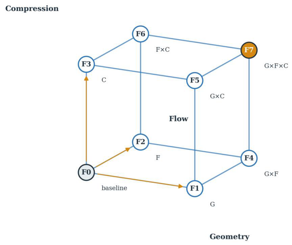
Figure 3.
The classical Modified Cam Clay yield curve and the real teardrop yield curve of Chatwong et al. [11] in normalized stress space, shown here for Kaolin Clay (=1.5, =1.17, Table 1 of [11]) because its parameters give the clearest teardrop shape for illustration. This figure is illustrative only; all factorial calculations in this study, including Table 4, use Boston Blue Clay’s own parameters (Ψ=1.4, Ω=0.93) throughout. The state point =1/OCR=0.2 (OCR=5) marked here is the same initial state used to evaluate the dilatancy ratio D in Section 3.1, independent of which soil’s curve is plotted.
Figure 3.
The classical Modified Cam Clay yield curve and the real teardrop yield curve of Chatwong et al. [11] in normalized stress space, shown here for Kaolin Clay (=1.5, =1.17, Table 1 of [11]) because its parameters give the clearest teardrop shape for illustration. This figure is illustrative only; all factorial calculations in this study, including Table 4, use Boston Blue Clay’s own parameters (Ψ=1.4, Ω=0.93) throughout. The state point =1/OCR=0.2 (OCR=5) marked here is the same initial state used to evaluate the dilatancy ratio D in Section 3.1, independent of which soil’s curve is plotted.
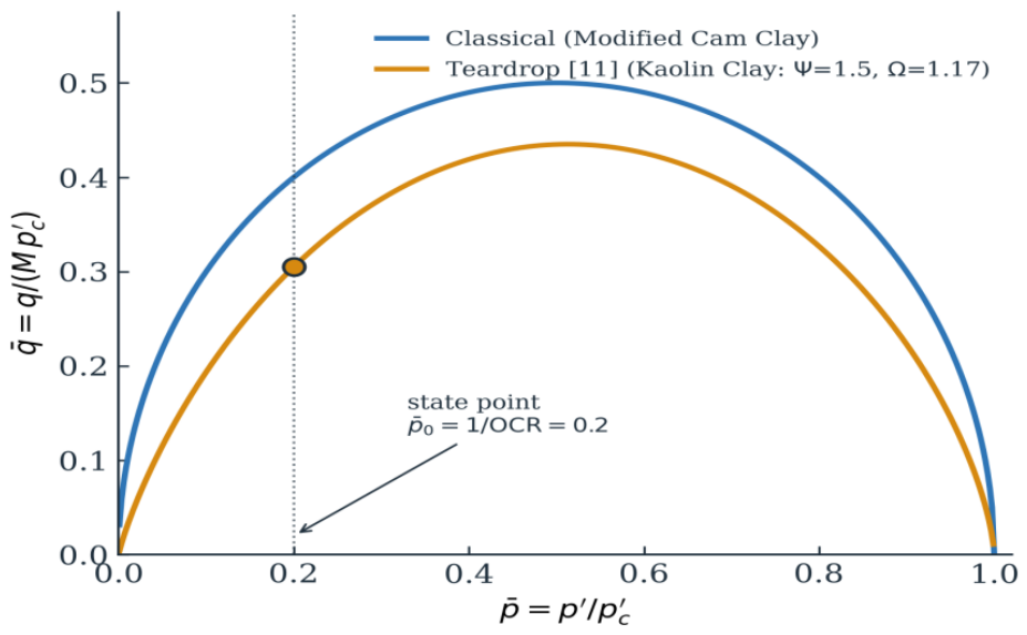

Table 4.
Response (accumulated over εₛᵖ=6) for the eight constitutive configurations (Boston Blue Clay, real parameters, OCR = 5).
Table 4.
Response (accumulated over εₛᵖ=6) for the eight constitutive configurations (Boston Blue Clay, real parameters, OCR = 5).
| Framework | Geometry | Flow | Compression | R = εᵥᵖ |
|---|---|---|---|---|
| F0 | Classical | Integer-order | Conventional | −0.13765 |
| F1 | Teardrop | Integer-order (ref. [11]) | Conventional | −0.08024 |
| F2 | Classical | Fractional | Conventional | −0.22057 |
| F3 | Classical | Integer-order | AJOP | −0.10821 |
| F4 | Teardrop | Fractional | Conventional | −0.21163 |
| F5 | Teardrop | Integer-order (ref. [11]) | AJOP | −0.07502 |
| F6 | Classical | Fractional | AJOP | −0.13368 |
| F7 | Teardrop | Fractional | AJOP | −0.13190 |
All eight entries in Table 4 are negative, reflecting net dilation from the initial state=0.2 used throughout Section 3.3, Section 3.4 and Section 3.5: every flow rule in this study predicts dilative behaviour at this starting state (Section 4.1). As shear proceeds, rises from 0.2 toward each framework’s own critical-state point —=0.5 for classical-integer flow, ≈0.341 for teardrop-integer flow, and ≈0.868 and 0.818 for the two fractional-flow combinations (Section 3.1) — where =0 and further accumulation cease. The magnitude of each entry in Table 4 therefore reflects how far the shared starting state sits from that particular framework’s own critical point, not a transition from contractive to dilative behavior partway through the path; no entry in Table 4 represents a sign error or numerical artefact.
From Table 4, the main effects and interaction indices (Equations 22–26) are:
R(F0)=−0.13765 is itself negative (net dilation, Section 4.1), so throughout Table 5 and Figure 4 and Figure 5, “% of |R(F0)|” means each quantity is divided by the magnitude |R(F0)| with its own sign preserved in the numerator, not by the signed value R(F0) itself; dividing by the signed value would flip every percentage’s sign relative to what is reported. This convention is used because it keeps the sign of each percentage matching the sign of the underlying quantity (e.g., ΔG>0 in both raw and percentage terms), which is more directly interpretable than the alternative.
Table 5.
Main effects and interaction indices, Boston Blue Clay, real parameters, OCR = 5.
| Quantity | Value | % of |R(F0)| |
|---|---|---|
| ΔG | +0.05741 | +41.7% |
| ΔF | −0.08292 | −60.2% |
| ΔC | +0.02944 | +21.4% |
| −0.04847 | −35.2% | |
| −0.02422 | −17.6% | |
| +0.05745 | +41.7% | |
| +0.01706 | +12.4% |
3.4. Sensitivity to Overconsolidation Ratio
Because a single state point cannot establish whether the interaction pattern in Table 5 is a robust feature or an artefact of one particular OCR, the same eight-framework evaluation was repeated for OCR=2–10, using the real Boston Blue Clay parameters throughout. OCR=2 (=0.5) is a degenerate case for the classical baseline, since p̄=0.5 is exactly the critical-state point of the Modified Cam Clay ellipse (=0 there), giving R(F0)≈0 and ill-defined percentages; it is excluded from the range reported below. For OCR=3–10, the pattern is stable and monotonic: ΔG is positive and shrinks with OCR (+94% at OCR=3 to +24% at OCR=10), ΔF is negative and shrinks in magnitude with OCR (−115% to −37%) while remaining the single largest quantity throughout, ΔC grows substantially with OCR (+1% to +43%) rather than staying negligible, is negative and shrinks with OCR (−75% to −21%), and — the flow×compression interaction — is consistently large (+37% to +43% over OCR=3–8) and comparable in magnitude to the main effects. remains smaller but not negligible (up to −19%), as does (up to +16% over OCR=3–8); the OCR=10 values of and are undefined, for the reason given at the end of this section. Robustness to yield-surface parameter choice is established by the second real soil in Section 3.5.
3.5. Cross-Check with a Second Soil: London Clay
Because every result reported so far uses a single soil, the same OCR=2–10 sweep was repeated for London Clay, the only other soil in this study’s set for which both the teardrop yield-surface parameters (Chatwong et al. [11], Table 1: Ψ=1.1, Ω=0.95; their ratio κ/λ=0.064/0.168=0.381 applied to =0.0586 from Table 3, giving κ=0.0223) and the AJOP compression parameters (Phonchamni et al. [31], Table 1: Γ=0.850, =0.135, R=530, θ=0.0058) are independently calibrated and real, rather than assumed. All other settings (p′c=600 kPa, εₛᵖ budget=6) were kept identical to the Boston Blue Clay case to isolate the effect of changing soil parameters alone.
The constant-λ quantities reproduce the Boston Blue Clay pattern exactly. At OCR=5, ΔF=−60.3% is again the largest single quantity, ΔG=+39.2% is positive as for Boston Blue Clay, and =−24.5% is negative and smaller in magnitude than ΔF; across OCR=3–10, ΔF runs from −115% to −37%, ΔG from +89% to +22%, and from −42% to −16% — the same trends, with slightly smaller magnitudes, as Boston Blue Clay. The compression-related quantities, by contrast, encounter the hardening singularity identified in Section 3.4 far earlier for this soil. Because London Clay’s AJOP transition is much sharper (θ=0.0058) and its reference stress high relative to the mean stresses used (R=530 kPa), (p′c)=κ already at p′c≈190 kPa: F6 crosses this singular point from OCR=4 upward and F7 from OCR=5, so the flow×compression interaction is defined only at OCR=3, where it is +67.2% of |R(F0)| — again the largest interaction, and larger than any Boston Blue Clay value; F3 crosses it from OCR=8 and F5 at OCR=10, so the compression main effect ΔC is defined over OCR=3–6, where it grows from +9.6% to +46.8% (compared with +1.2% to +27.8% for Boston Blue Clay over the same range), and over the same range grows to −27%. The ranking of terms — ΔF and largest where both are defined, smaller and shrinking with OCR, ΔC substantial and growing with OCR — is therefore not a Boston Blue Clay-specific artefact; at the same time, the second soil demonstrates that the AJOP hardening singularity is soil-dependent and can intrude well inside the moderate-OCR range rather than only at its edge. This remains a two-soil check, not a general validation across soil types — both soils used here happen to be relatively low-plasticity, moderate-OCR marine/glacial clays for which Chatwong et al. [11] provide real parameters — and extending it to a wider range of plasticity indices remains future work (Section 5).
That the interaction pattern varies smoothly and monotonically with OCR over this range is consistent with independent microstructural evidence that OCR itself produces a graded, rather than abrupt, change in soft clay fabric: Kong et al. [33] used SEM imaging to show that the fractal dimension of soft clay pore structure decreases smoothly with increasing OCR under cyclic loading, with no discontinuity reported across the OCR range they tested. This does not validate the specific magnitudes reported here, but it is at least consistent with treating OCR as a state variable that shifts constitutive behavior gradually rather than discontinuously, which is an implicit assumption of the sensitivity analysis in this section.
This sensitivity analysis also surfaced a feature not visible in the single-state evaluation: the teardrop-plus-integer-order flow ratio from Chatwong et al. [11] passes through zero at 0.341 for Boston Blue Clay’s Ω=0.93, a phase-transformation point at which flow is purely deviatoric. Under the associated-flow dilatancy ratio derived in Section 3.1.1, every framework’s shear-strain-controlled path from =0.2 rises toward, and stabilises smoothly at, its own flow rule’s equilibrium point —=0.5 for classical-integer flow, for teardrop-integer flow, and the wet-side values ̄p≈0.868 and 0.818 for the two fractional-flow combinations (Section 3.1) — and no oscillation or clamp-hugging behaviour was observed for any framework over OCR=3–8. At OCR=10, however, one framework fails structurally rather than numerically. Because (p′c)→0 at low preconsolidation stress (Section 2.6), the effective hardening modulus −κ necessarily vanishes at a finite p′c — for the Boston Blue Clay parameters of Table 3, at p′c≈67.4 kPa — where the hardening law of Equation (15) is singular. At OCR=10 (p′=60 kPa) this singular point corresponds to ̄p=p′/p′c≈0.891, and the classical-fractional equilibrium (̄p≈0.904 at α(10)=0.562) lies beyond it: F6’s path must cross the singularity before reaching equilibrium, and it does not converge at any step count tested — runs at =60,000–200,000 agree to three to four figures but a run at 400,000 departs from them, an apparent convergence that is spurious. The teardrop-fractional equilibrium (̄p≈0.862) lies just inside the singular point, and F7 converges normally. The compression-related interaction indices and , which involve F6, are therefore reported over OCR=3–8 only; every quantity not involving F6 (ΔG, ΔF, ΔC, , ) is converged over the full OCR=3–10 range, and all results in Section 3.3, Section 3.4 and Section 3.5 use =60,000. This hardening singularity is a structural property of embedding AJOP as the hardening modulus: the same low-stress flattening that gives AJOP its Γ-bound (Section 2.6) guarantees that its tangent falls below the swelling index at sufficiently low p′c. Section 3.5 shows that for a second soil it intrudes at much lower OCR, and Section 4.6 shows that a proportional-κ variant of the hardening law removes it entirely.
4. Discussion
The robust, path-integrated results of Section 3.3, Section 3.4 and Section 3.5, obtained using real yield-surface parameters from Chatwong et al. [11] and real AJOP parameters from Phonchamni et al. [31], give the following picture. The flow main effect ΔF is the largest single quantity at every OCR tested (−37% to −115% of |R(F0)| across OCR=10–3), followed by the geometry main effect ΔG (+24% to +94%, shrinking with OCR) and the flow×compression interaction (+37% to +43% for Boston Blue Clay over OCR=3–8, roughly stable; +67% for London Clay at OCR=3, the only overconsolidation ratio at which it is defined for that soil — Section 3.4 and Section 3.5). The geometry×flow interaction is negative throughout and shrinks in magnitude as OCR increases (−21% to −75%). The compression main effect ΔC, rather than staying small, grows substantially with OCR (+1% to +43% for Boston Blue Clay across OCR=3–10; +10% to +47% for London Clay across OCR=3–6, Section 3.5) and is comparable in magnitude to ΔG at high OCR. No single main effect or interaction dominates every other throughout the range.
This is a more interesting result than the framework’s original motivation anticipated. Section 1 motivated compression as a third component deserving the same constitutive status as geometry and flow; Section 3 confirms that expectation more strongly than the paper originally set out to claim. Compression’s main effect ΔC grows with OCR rather than staying negligible, and its interaction with flow, , is consistently one of the two or three largest quantities in the entire factorial design — comparable in magnitude to the geometry×flow interaction , and larger than it from OCR=5 upward. AJOP’s own reported strength, large settlement-error reduction at shallow depth [30,31], is a statement about compression-alone behavior under oedometer loading, a different loading path and response quantity from the shear-dominated one evaluated here; the present result is consistent with that strength rather than independent of it — compression’s influence propagates into the shear response primarily through its interaction with the flow rule (), not as a standalone effect (ΔC alone is smaller than at every OCR tested), which is itself a specific, falsifiable claim about how AJOP’s compression law couples to the rest of this framework. The same embedding also carries a structural cost that Section 3.4 and Section 3.5 make explicit: because →0 at low stress, the effective hardening modulus −κ necessarily vanishes at a finite, soil-dependent preconsolidation stress (≈67 kPa for Boston Blue Clay, ≈190 kPa for London Clay), beyond which Equation (15) is singular — physically, the point at which the virgin tangent compressibility falls below the recompression index. The Γ-bound presented in Section 2.6 as AJOP’s low-stress advantage over a constant λ therefore has a precise flip side when AJOP is embedded as a hardening modulus rather than used as a settlement equation, and any sufficiently dilative path can reach it. A regularisation, or an explicit restriction of the framework’s domain of validity to p′c above the singular stress, is required before the AJOP-hardening branch of this framework can be used predictively; Section 4.6 implements one such modification — tying the swelling index to the AJOP tangent at the calibrated ratio κ/λ — and finds that it removes the singularity by construction while leaving the factorial ranking intact.
MIT-E3 [22] and MIT-S1 [23] remain a relevant point of comparison for : both are complete architectures in which yield geometry and flow were calibrated together, consistent with a non-trivial geometry×flow interaction being a real feature of coupled constitutive design rather than a modelling artefact, even though is not the largest such interaction found here. The unified hardening (UH) model of Yao, Hou and Zhou [7] ties yield-surface size to a hardening parameter, which would predict some geometry–compression coupling; the present is small at low OCR but grows to −19% by OCR=8–10, though UH does not use the same shear-strain-controlled response quantity and so is not a direct test of the same claim. The flow×compression interaction , for which no directly comparable coupled architecture in the literature reviewed here isolates the same pairing, is the largest interaction term found in this study and is not directly anticipated by any of the models compared against in this Discussion.
On the flow side, Sun and co-workers’ stress-fractional plasticity [25,26,28] and the Qu, Sun and Sumelka review [27] evaluate the fractional operator on a fixed, usually classical, yield surface, and so could not previously have observed , whatever its true size — the present result extends the domain over which their own stated mechanism (fractional differentiation of the yield function) has actually been tested, rather than confirming or contradicting a claim that literature made. A more direct point of contact is Chatwong et al. [11] itself: their own non-associated flow rule D=M−η (Section 2.3) was found here to pass through zero at a genuine phase-transformation point ρ̄*=exp(−1/Ω), which the fractional alternative proposed in this paper (F4, F7) does not exhibit. This is a concrete, structural difference between the two flow treatments on the same yield surface, not merely a difference in numerical convenience, and it is the kind of observation that the present factorial framework was designed to surface.
These results should still be read as a first, transparent test of the interaction hypothesis, not a validated constitutive prediction ready for design use. The teardrop yield function is now the verified closed form of Chatwong et al. [11] (Section 2.2), and the flow-integration scheme is now a genuine incremental path integration rather than a single-state algebraic proxy (Section 3.1), which closes two of the three limitations identified in earlier review of this work. The third — that all results rest on one soil and one loading path — is now only partly open. A second soil (London Clay, Section 3.5) reproduces the same ranking of terms (ΔF and largest where defined, smaller and shrinking with OCR, ΔC substantial and growing with OCR) with somewhat different magnitudes and with the compression-related quantities bounded above in OCR by the AJOP hardening singularity (Section 3.4 and Section 3.5), and a second, approximate loading path (undrained shear, Section 4.3) shows all eight frameworks reaching stable equilibria at the same D=0 points as the drained path, with the constant-λ quantities carrying over identically and the compression-related quantities suppressed several-fold — a path effect the drained results alone do not reveal. What remains genuinely untested is sensitivity to soil plasticity across a wider range than these two moderate-plasticity soils span, stress path types beyond drained and approximately-undrained (K0, cyclic), and the exact numerical realisation of the state-dependent stress-length-scale convention specified in Equation (8), and the effect of re-evaluating the fractional order from the evolving state along each path rather than holding it at its initial-state value (Section 2.9). What the present results do establish is that no single main effect or interaction dominates the factorial design; the flow main effect and the flow×compression interaction are consistently the largest quantities, compression’s role is substantial and grows with overconsolidation ratio rather than being negligible, and the geometry×flow interaction carries over to the approximate undrained loading path unchanged — exactly so, since within these two idealised schemes the constant-λ quantities are fixed by the same D=0 equilibrium points (Section 4.3) — while compression’s role is suppressed several-fold there, a genuine path effect driven by the elastic term dominating the undrained volumetric modulus. On this evidence the geometry×flow coupling is the more path-independent of the two interactions examined here, with the caveat that its undrained persistence is structural to the two schemes compared rather than an independent test.
4.1. Where the Classical and Teardrop Flow Rules Agree and Disagree on Dilatancy
Section 3.1.1 derives the classical associated-flow dilatancy ratio as , which reduces to the standard critical-state result . With this sign, classical MCC predicts <0 (dilative) throughout the dry side (<0.5), matching standard critical-state theory (e.g., Roscoe and Burland) and the well-documented tendency of real heavily overconsolidated clay to dilate on shearing rather than contract [1,5,19,20]. The teardrop surface’s own non-associated flow rule [11] gives the same sign (dilative) throughout most of the dry side too.
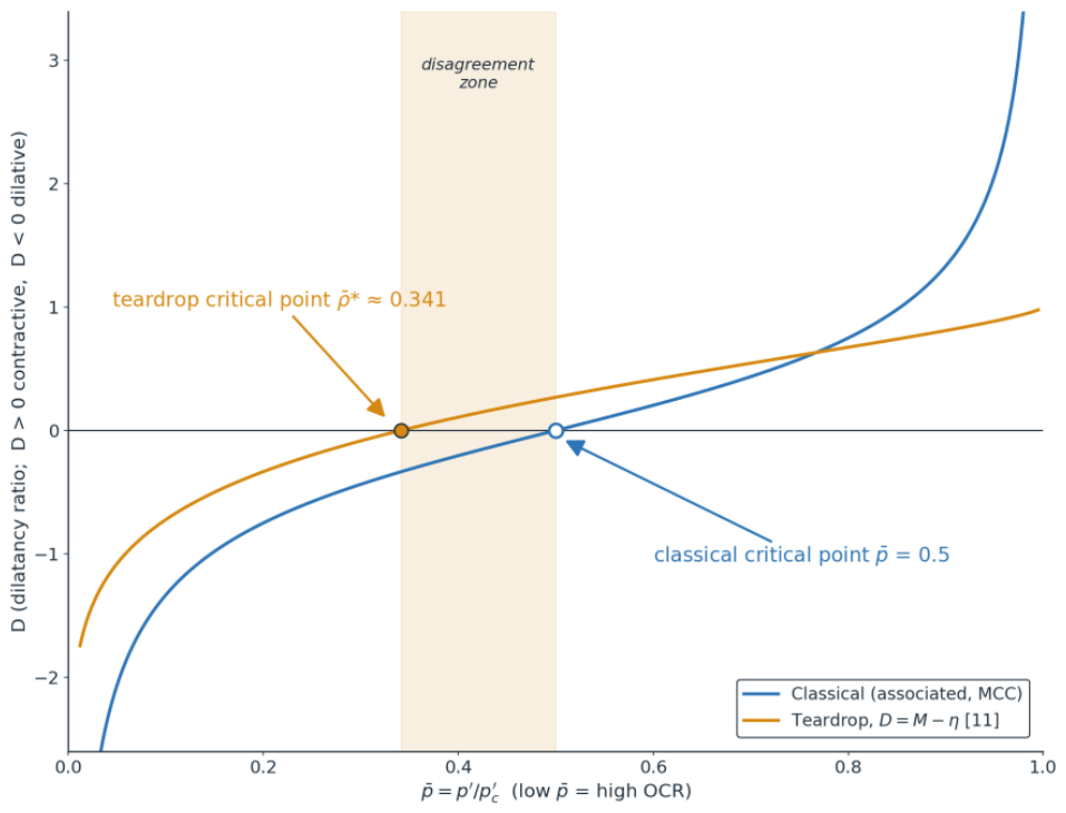
What the comparison shows is a genuine, more specific disagreement: the two flow rules agree in sign almost everywhere, but not because they agree on where the critical state lies. Classical MCC’s own critical-state point is at =0.5 (where =0 identically, independent of any soil parameter); the teardrop flow rule’s critical-state point is at ≈0.341 for Boston Blue Clay (Section 2.4), a different, soil-dependent value. Between these two points (0.341<<0.5), the two flow rules disagree in sign: classical MCC still predicts dilative behavior there, while the teardrop flow rule already predicts contractive behavior. Outside this narrow band, the two agree — both dilative for <0.341, both contractive for >0.5.
Figure 6.
Dilatancy ratio D versus p̄ for the classical associated flow rule (Section 3.1.1) and the teardrop surface’s non-associated flow rule [11] (real Boston Blue Clay parameters, =1.4, =0.93). >0 is contractive, <0 is dilative. The two flow rules disagree in sign only in the shaded band between their respective critical-state points (≈0.341 and =0.5); outside this band they agree.
Figure 6.
Dilatancy ratio D versus p̄ for the classical associated flow rule (Section 3.1.1) and the teardrop surface’s non-associated flow rule [11] (real Boston Blue Clay parameters, =1.4, =0.93). >0 is contractive, <0 is dilative. The two flow rules disagree in sign only in the shaded band between their respective critical-state points (≈0.341 and =0.5); outside this band they agree.
The state points explored in Section 3.3, Section 3.4 and Section 3.5 (=1/OCR, OCR≥3, so ≤0.333) fall inside the agreement zone — both flow rules predict dilative behavior at the starting state for every OCR used in this study’s factorial design. This means the substantial numerical differences between classical- and teardrop-geometry frameworks reported in Table 4 and Table 5 (ΔG, , and so on) are not explained by a sign disagreement at the starting state; they arise from the different magnitudes and different critical-state points the two flow rules predict as the state evolves under load, which is exactly the mechanism the factorial design in this paper is built to isolate. The disagreement band identified here is a genuine, quantitatively specific difference between Chatwong et al.’s [11] flow rule and the classical associated alternative, but it is a narrower and more precise finding than a blanket sign check would suggest.
4.2. Reproducing Chatwong et al.’s Own Validation for All Four Calibrated Soils
The qualitative sign check in Section 4.1 can be extended into a direct, quantitative reproduction of the validation Chatwong et al. [11] already carried out for their own model, because both halves of that comparison are available: real undrained triaxial stress paths, compiled from the primary sources Chatwong et al. [11] present in their Figure 2 (Pestana, Whittle and Gens [34] for Boston Blue Clay, Wroth and Loudon [35] for Kaolin Clay, Gens [36] for Lower Cromer till, and Gasparre [37] for London Clay), and Chatwong et al.’s [11] own computed model-prediction curves for each tested OCR — not a static yield surface read off at one state, but the full stress-path prediction their model produces when integrated with hardening, for the same soils and the same OCR values as the test data (four to eight OCR values per soil, 20 paths, 379 points in total). Both are used here exactly as reported, with no re-fitting or re-derivation on this paper’s part.
Figure 7 plots the real test data against Chatwong et al.’s [11] own prediction curves for each soil and OCR. The fit is close throughout: the mean absolute error between predicted and measured , taken over all 379 points, is 0.049 (median 0.024), and three-quarters of all points agree to within 0.05. The one systematic exception is the OCR≈2 curve in several soils, where the mean error rises to about 0.13 — visibly greater scatter than the other OCR values, consistent with the greater scatter around the prediction line visible at OCR=2 in Chatwong et al.’s [11] own published Figure 14 for London Clay. Excluding OCR≈2, the mean absolute error over the remaining 311 points is 0.031.
This close agreement is Chatwong et al.’s [11] own validation, reproduced here rather than established anew: the yield surface, its embedded flow rule, and the hardening law that together produce this prediction curves are entirely [11]’s, calibrated and validated in their own study before this paper adopted them. Chatwong et al.’s [11] own integrated prediction curves, rather than a static yield surface evaluated at one state, are the appropriate comparison here because the critical state each curve reaches depends on OCR: for Boston Blue Clay, for example, the terminal ̄p ranges from ≈0.40 at OCR=1 to ≈0.28 at OCR=8, rather than a single fixed ==0.341 as the flow rule’s own zero-crossing point alone would suggest. A comparison against the static yield surface would compare real data to the wrong quantity; the path-integrated predictions used here avoid that mismatch.
What this section establishes, and what it does not, should be stated precisely. It confirms that the yield surface and flow rule this paper adopts from Chatwong et al. [11] are well supported by real undrained triaxial data across four independently calibrated soils — a property of the borrowed component, demonstrated by its original authors and reproduced here for transparency, not a new result of this paper. It does not validate the fractional flow rule, the AJOP-based hardening law, the 2×2×2 factorial design, or the incremental path-integration scheme in Section 3, all of which are this paper’s own contributions and remain checked only against internal consistency (Section 3) and the qualitative sign check (Section 4.1).
4.3. A Second Loading Path: Approximate Undrained Shear
All results reported in Section 3.3, Section 3.4 and Section 3.5 use a single loading path (drained shear at constant p′, Section 3.1). As a check of whether the interaction pattern also holds under a different loading condition, an approximate undrained path was implemented for the same eight frameworks at OCR=5. Undrained conditions were enforced through the standard critical-state elastic relation (constant total volumetric strain, i.e., plastic volumetric strain compensated by elastic volumetric strain via , with =2.059 — Chatwong et al.’s [11] own reported value for Boston Blue Clay, Table 1 — held fixed as an approximation) combined with the same hardening law used elsewhere in this study. Combining these two relations collapses to a single ordinary differential equation in ̄p alone — — which avoids the compounding error of tracking p′ and as separate multiplicatively-updated quantities.
Under the dilatancy ratios of Section 3.1.1, all eight frameworks reach a stable equilibrium under this approximate undrained path. The four integer-order-flow frameworks stabilise at the same critical-state points identified in the drained results (=0.5 for F0/F3, classical; ≈0.341 for F1/F5, teardrop), and the four fractional-flow frameworks stabilise at exactly the same wet-side equilibria as under the drained path (≈0.868 for F2/F6, ≈0.818 for F4/F7). The coincidence is exact rather than approximate: both loading schemes share the same dilatancy function , and every equilibrium is a root of =0 — the two paths differ only in the positive factor multiplying in the update equation, which sets how fast the equilibrium is approached but cannot move it. No framework diverges toward either the } or clamp under this loading path: fractional-order and integer-order flow behave alike here, each reaching a stable equilibrium regardless of yield geometry.
Because every framework stabilises within a comparable portion of the εₛᵖ=6 budget, a direct R/percentage comparison across all eight frameworks is meaningful. For the constant-λ configurations the comparison is exact by construction: both schemes obey R=−C·ln(̄p_end/̄p₀) with a path-specific positive constant C that cancels from every percentage, so ΔG=+41.7%, ΔF=−60.2% and =−35.2% reproduce the drained percentages identically. The compression-related quantities, by contrast, are strongly suppressed under this loading path but not eliminated: ΔC=+2.6%, I_GC=−2.2%, =+9.1% and =+0.7%, all with the same signs as the drained results but four to eight times smaller in magnitude (drained: ΔC=+21.4%, =+41.7%), because the undrained modulus is dominated by the elastic term (1+e₀)/κ≈84, which is common to all eight frameworks and dilutes the difference between the two hardening laws. Two points of numerical bookkeeping follow from the dynamics: the constant-λ quantities are converged already at =6,000, while the compression-related quantities require ≈200,000 (confirmed against 600,000), because equilibrium is reached within roughly 1% of the strain budget and the AJOP-versus-constant-λ difference accrues entirely in that short transient. The geometry×flow interaction carrying over unchanged is therefore a structural property of the two schemes compared, rather than an independent test of path-independence; the several-fold suppression of compression’s role is the genuine path effect — consistent with compression’s influence operating primarily through the volumetric hardening pathway that undrained conditions largely suppress. This is a single additional loading path, not a general demonstration, and the pore-pressure and stress-path evolution this simplified single-ODE approximation omits should be treated properly before the path-dependence suggested here is considered established; that fuller undrained assessment is left for future work (Section 5).
4.4. Decomposing the Geometry Effect: Yield-Surface Shape Versus Flow-Rule Type
F1 (teardrop, Table 2) differs from F0 (classical) in two respects simultaneously, not one: the yield-surface shape changes from the MCC ellipse to the teardrop surface, and the flow rule changes from the associated normal used for F0 to Chatwong et al.’s [11] own non-associated D=M−η, which is the flow rule actually proposed alongside their yield surface (Section 2.3) rather than the associated normal to the teardrop surface itself. The reported ΔG (Table 5) is therefore a combined geometry-and-flow-rule-type effect, not a geometry effect in isolation, and the factorial design’s orthogonality claim should be read with this in mind.
To isolate the shape effect alone, a supplementary configuration was evaluated using associated flow on the teardrop surface itself — D=−g′(̄p) for the real teardrop , the same construction used for F0’s classical , applied to the teardrop surface instead of [11]’s own flow rule. Comparing this configuration against F0 isolates the shape-only effect ΔG′, holding flow-rule type (associated) fixed across both geometries. Across OCR=3–10 for Boston Blue Clay, ΔG′ is +1.3% to +5.2% of |R(F0)| — consistently about 5.5% of the reported, combined ΔG (+23.7% to +94.2% over the same range). Yield-surface shape alone, in other words, accounts for only a small fraction of the geometry main effect reported in Table 4 and Table 5; the great majority of ΔG reflects the change from associated to Chatwong et al.’s [11] non-associated flow rule that accompanies the geometry change in this study’s factorial design, not the change in surface shape itself.
This does not invalidate the factorial results in Section 3.3, Section 3.4 and Section 3.5, which correctly report the effect of moving from F0 to F1 as defined in Table 2 — a specific, stated combination of geometry and flow rule, not an abstract geometry axis. It does mean ΔG and should be read as effects of adopting the teardrop-plus- combination specifically, rather than of yield-surface shape in isolation, and that a full decomposition separating shape from flow-rule type across all eight frameworks — not only F0 versus F1 — is left for future work.
4.5. Sensitivity to the Fractional Order α
The state-dependent fractional order uses =0.55 and k=0.40 (Section 2.5); these two constants are chosen rather than fitted to data for either soil used in this study, and no source in the fractional-plasticity literature this paper draws on [24,25,26,27,28] reports values for this specific functional form, since it is this paper’s own proposal. Because these constants set ≈0.641, the value used throughout Section 3.3 and Section 3.4, it is necessary to check whether the factorial findings depend on this specific choice or hold more generally across plausible α.
Figure 8 shows the main effects and the two largest interactions recomputed at OCR=5 with α held fixed at values from 0.3 to 0.9, spanning well beyond the range actually takes across OCR=1–10 (approximately 0.56 at OCR=10 to 0.75 at OCR=3 by the formula above, approaching 1 as OCR→1). ΔG and ΔC do not depend on α at all, since F1/F3’s own flow rules do not use the fractional operator; ΔF and , which do involve fractional flow, vary substantially with α (ΔF from −72.6% at α=0.3 to −26.9% at α=0.9; from +52.0% to +16.7% over the same range), while is comparatively stable (−39.5% to −33.5%). Every quantity’s sign is unchanged across the entire α=0.3–0.9 range tested. The specific ranking — ΔF largest, followed by , then ΔG — holds for α up to about 0.7–0.8. This covers the α values used at OCR≥4 but sits at its upper edge at OCR=3, where α(3)=0.75; the OCR=3 drained result itself (Section 3.4, where ΔF=−115% is the largest quantity) confirms the ranking holds there. The ranking inverts at α=0.9, where ΔG and become the largest terms instead. The qualitative claim that no single quantity dominates the factorial design (Section 3.3 and Section 3.4) is therefore robust across the tested range; the specific claim that ΔF is the single largest quantity is robust for as actually used, but would not necessarily hold under a different, unfitted choice of α_min and k that pushed α toward 0.9 or beyond.
4.6. A Proportional-κ Variant: Removing the Hardening Singularity
The hardening singularity identified in Section 3.4 and Section 3.5 arises from the combination of a stress-dependent virgin modulus (p′c) with a constant swelling index κ: because →0 at low stress while κ does not, their difference must vanish at a finite preconsolidation stress. This suggests a minimal, physically motivated modification that removes the singularity at its root rather than regularising it numerically: tie the swelling index to the virgin tangent at the calibrated ratio, κ(p′c)=r·(p′c) with r=κ/λ taken from Chatwong et al. [11] (r=0.196 for Boston Blue Clay, r=0.381 for London Clay), applied pointwise rather than once. The effective hardening modulus becomes =(1−r)· (p′c), strictly positive everywhere in the admissible domain, and the physical requirement that recompression stiffness cannot exceed virgin stiffness is enforced at every stress rather than only at the calibration point. For the constant-λ configurations the modification changes nothing — κ=r·λ_LF is the same constant as before — so F0, F1, F2 and F4, and with them ΔG, ΔF and , are identical to Section 3.3, Section 3.4 and Section 3.5.
Under this variant every compression-related quantity is defined over the full OCR=3–10 range for both soils, including the previously non-convergent F6 cases, which now converge normally (Boston Blue Clay at OCR=10: agreement to three to four figures between =60,000 and 200,000, the path stabilising unobstructed at its fractional equilibrium ≈0.904). The compression-related magnitudes shrink by roughly 15–20% relative to the constant-κ results but keep their signs and trends: at OCR=5 for Boston Blue Clay, ΔC=+17.2% (constant-κ: +21.4%), =+33.6% (+41.7%), I_GC=−14.2% (−17.6%) and =+10.0% (+12.4%); across OCR=3–10, ΔC grows from +1.0% to +34.8% and stays roughly stable at +28% to +34% for Boston Blue Clay, and ΔC grows from +6.0% to +41.4% and runs from +42% to +30% for London Clay. The qualitative conclusions of Section 3.3, Section 3.4 and Section 3.5 are unchanged: no single main effect or interaction dominates, and ΔF remains the largest single quantity at every point tested except London Clay at OCR=10, where ΔC (+41.4%) marginally overtakes it (−36.8%). The variant also has an exact structural property: because λ_eff equals (1−r) times the branch modulus uniformly across all eight configurations, the factor (1−r) cancels from every percentage in the factorial design, so the variant’s normalised results are independent of r altogether (verified numerically for r=0.10–0.30).
Two conclusions follow. First, the hardening singularity of Section 3.4 and Section 3.5 is a property of the constant-κ embedding, not of the AJOP law itself: a modification that leaves AJOP untouched and changes only the swelling-index policy removes it for both soils. Second, this variant is presented for the drained factorial only; under undrained conditions κ also enters the elastic volumetric relation (Section 4.3), and a stress-dependent κ requires a consistent treatment of the elastic law before the undrained results can be repeated, which is left for future work (Section 5).
5. Conclusions
This paper formulated a three-component constitutive architecture combining the verified closed-form teardrop yield surface of Chatwong et al. [11], a state-dependent stress-fractional flow rule, and a nonlinear hardening modulus derived analytically from the AJOP compression equation, and tested the resulting geometry–flow–compression interaction hypothesis using a 2×2×2 factorial design integrated incrementally along a shear-strain-controlled stress path. Ten findings emerge. First, the AJOP compression law was shown analytically to approach Γ as a physical upper bound on void ratio at low stress, while its tangent compression modulus (Equation 13) tends to zero, unlike a constant compression index, which is bounded in neither quantity; this distinction was numerically material using real fitted parameters for three clays (Table 3). Second, no single main effect or interaction dominates the 2×2×2 factorial design: the flow main effect ΔF is the largest single quantity at every OCR tested for Boston Blue Clay (−37% to −115% of |R(F0)| across OCR=10–3), the geometry main effect ΔG is the second largest and shrinks with OCR, and the flow×compression interaction (+37% to +43% for Boston Blue Clay over OCR=3–8; +67% for London Clay at OCR=3, Section 3.5) is consistently comparable to the geometry×flow interaction — exceeding it in magnitude from OCR=5 upward — which is itself negative and shrinks in magnitude as OCR increases (−21% to −75% for Boston Blue Clay). Third, and unexpectedly, compression’s role is substantial and grows with OCR rather than staying negligible: the main effect ΔC rises from about 1% to 43% of |R(F0)| across OCR=3–10 for Boston Blue Clay, and its interaction with flow () is one of the two or three largest quantities in the entire design wherever it is defined; compression does not behave as an essentially additive component. Fourth, the sensitivity analysis surfaced a genuine phase-transformation singularity in Chatwong et al.’s own non-associated flow rule ( at ) that the fractional alternative proposed here does not exhibit — a structural, not merely numerical, difference between the two flow treatments. Fifth, a second, previously unreported structural singularity was identified in the AJOP-based hardening law itself: because →0 at low stress, the effective hardening modulus −κ vanishes at a finite, soil-dependent preconsolidation stress (p′c≈67 kPa for Boston Blue Clay, ≈190 kPa for London Clay), where Equation (15) is singular; frameworks whose flow-rule equilibrium lies beyond this point do not converge at any step count (F6 at OCR=10 for Boston Blue Clay; F6 from OCR=4 and F7 from OCR=5 for London Clay), which bounds the overconsolidation range over which the compression-related interaction indices are defined and is the precise flip side of the Γ-bound identified in the first finding; a proportional-κ variant (Section 4.6), which ties the swelling index to the AJOP tangent at the calibrated ratio κ/λ, removes the singularity by construction, leaves the constant-λ half of the design unchanged, and reproduces the same ranking with compression-related magnitudes roughly 15–20% smaller — identifying the singularity as a property of the constant-κ embedding rather than of the AJOP law itself. Sixth, the same ranking of terms reproduces for a second, independently calibrated soil (London Clay, Section 3.5) over the range where each quantity is defined: ΔF and remain the largest quantities, is negative and shrinks with OCR, and ΔC grows substantially with OCR (+10% to +47% over OCR=3–6, larger in magnitude than for Boston Blue Clay over the same range). Seventh, the classical associated flow rule and Chatwong et al.’s [11] own non-associated flow rule D=M−η agree in sign almost everywhere — both dilative on the dry side, both contractive on the wet side — and disagree only in a narrow band between their two different critical-state points (ρ̄*≈0.341 and p̄=0.5); the state points explored in this study’s factorial design fall outside that band, so the numerical differences between classical- and teardrop-geometry frameworks in Table 4 and Table 5 reflect differences in magnitude and evolution, not a sign disagreement at the starting state (Section 4.1). Eighth, an approximate undrained check (Section 4.3) shows that every one of the eight frameworks reaches a stable equilibrium under this loading path, at exactly the same equilibrium points as under the drained path — an exact property, since both schemes share the same dilatancy function and every equilibrium is a root of D=0; the constant-λ percentages carry over identically for the same structural reason (ΔG=+41.7%, ΔF=−60.2%, =−35.2%), while the compression-related quantities are suppressed several-fold rather than eliminated ( from +41.7% to +9.1%, ΔC from +21.4% to +2.6%), in contrast to their substantial drained-path role (Section 3.3, Section 3.4 and Section 3.5) — a genuine path effect, driven by the elastic term (1+e₀)/κ dominating the undrained volumetric modulus. This suggests compression’s interactive role operates mainly through the drained volumetric-hardening pathway, though this rests on a single additional, simplified loading path and should not yet be generalised. Ninth, Chatwong et al.’s [11] own validation of the teardrop yield surface and its embedded flow rule is reproduced directly against 379 points from 20 real undrained triaxial stress paths across all four calibrated soils (Section 4.2), using [11]’s own computed prediction curves rather than a static yield surface: agreement is close throughout (mean absolute error 0.049 in ̄q, three-quarters of points within 0.05), with more scatter at OCR≈2 consistent with [11]’s own published results. Tenth, the geometry main effect ΔG, as reported in Table 4 and Table 5, combines a yield-surface shape change with a flow-rule type change (associated to Chatwong et al.’s [11] own non-associated ); a supplementary check holding flow-rule type fixed (Section 4.4) finds that shape alone accounts for only about 5.5% of the reported ΔG across OCR=3–10, so ΔG and should be read as effects of the specific teardrop-plus- combination this study’s factorial design uses, not of yield-surface shape in isolation. The primary limitations of this version are that the main factorial evaluation still rests on one primary soil (Boston Blue Clay) and one initial-OCR sweep, with a second soil (Section 3.5) and a second, approximate loading path (Section 4.3) offered only as limited cross-checks rather than full replications of Section 3.3 and Section 3.4; the numerical scheme in Section 3 only approximates the state-dependent stress-length-scale convention specified in Equation (8) rather than implementing it exactly, and holds the fractional order fixed at its initial-state value along each path (Section 2.9 and Section 3.1); and no direct comparison of this paper’s own incremental, path-integrated predictions against digitized triaxial data has yet been made — though the yield surface and flow rule those predictions are built on have Chatwong et al.’s [11] own quantitative validation against real undrained triaxial data reproduced here for all four calibrated soils (Section 4.2). Future work should extend the factorial evaluation to additional soils and stress paths, implement the state-dependent stress-length-scale convention exactly rather than by fixed-step approximation, re-evaluate the fractional order from the evolving state along each path, extend the proportional-κ variant of Section 4.6 to a thermodynamically consistent stress-dependent elastic law and to the undrained relation, extend the approximate undrained check to a proper treatment of pore pressure and stress-path evolution, and compare predicted stress-strain and dilatancy curves against published triaxial data before the interaction hypothesis can be considered validated rather than demonstrated.
Supplementary Materials
The following supporting information can be downloaded at the website of this paper posted on Preprints.org. The calculation workbook used to reproduce Table 4 and Table 5 and Figure 1 and Figure 3–5 (FF_calculator.xlsx, with live formulas for all eight F0–F7 frameworks, a built-in consistency check based on the closed-form identity of Section 3.1, and a static reference table for the OCR sensitivity sweep) is provided as Supplementary File S1. A self-testing Python script that independently reproduces Table 4 and Table 5, the OCR sensitivity sweep, and the calculations of Section 4.3, Section 4.4, Section 4.5 and Section 4.6 (ff_canonical.py) is provided as Supplementary File S2.
Author Contributions
Conceptualization, N.K. and T.C.; methodology, N.K. and T.C.; software, T.C.; validation, N.K., and T.C.; formal analysis, N.K.; investigation, T.C.; resources, S.E. and A.K.; data curation, T.C.; writing—original draft preparation, N.K.; writing—review and editing, N.K., A.K., S.E. and S.S.; visualization, S.S., A.K. and S.E.; supervision, A.K. and S.E.; project administration, N.K.; funding acquisition, N.K. All authors have read and agreed to the published version of the manuscript.
Funding
This research was funded by Mahasarakham University.
Institutional Review Board Statement
Not applicable.
Informed Consent Statement
Not applicable.
Data Availability Statement
The original contributions presented in this study are included in the article and its Supplementary Materials (calculation workbook, File S1, and self-testing Python script, File S2). Further inquiries can be directed to the corresponding author.
Acknowledgments
The authors gratefully acknowledge Mahasarakham University for its support in all aspects of this research.
Conflicts of Interest
The authors declare no conflicts of interest.
References
- Roscoe, K.H.; Schofield, A.N.; Wroth, C.P. On the yielding of soils. Géotechnique 1958, 8, 22–53. [CrossRef]
- Roscoe, K.H.; Burland, J.B. On the generalized stress–strain behaviour of ‘wet’ clay. In Engineering Plasticity; Heyman, J., Leckie, F.A., Eds.; Cambridge University Press: Cambridge, UK, 1968; pp. 535–609.
- Hvorslev, M.J. Über die Festigkeitseigenschaften gestörter bindiger Böden; Ingeniørvidenskabelige Skrifter A, No. 45; Danmarks Naturvidenskabelige Samfund: Copenhagen, Denmark, 1937.
- Parry, R.H.G. Triaxial compression and extension tests on remoulded saturated clay. Géotechnique 1960, 10, 166–180. [CrossRef]
- Atkinson, J.H.; Bransby, P.L. The Mechanics of Soils: An Introduction to Critical State Soil Mechanics; McGraw-Hill: London, UK, 1978.
- Mita, K.A.; Dasari, G.R.; Lo, K.W. Performance of a three-dimensional Hvorslev–Modified Cam Clay model for overconsolidated clay. International Journal of Geomechanics 2004, 4, 296–309. [CrossRef]
- Yao, Y.P.; Hou, W.; Zhou, A.N. UH model: three-dimensional unified hardening model for overconsolidated clays. Géotechnique 2009, 59, 451–469. [CrossRef]
- Collins, I.F.; Yu, H.S. Undrained cavity expansion in critical state soils. International Journal for Numerical and Analytical Methods in Geomechanics 1996, 20, 489–516.
- Schädlich, B.; Schweiger, H.F. Modelling the shear strength of overconsolidated clays with a Hvorslev surface. geotechnik 2014, 37, 47–56. [CrossRef]
- Janda, T.; Šejnoha, M. Formulation of generalized Cam Clay model. Engineering Mechanics 2006, 13, 367–384.
- Chatwong, T.; Kaewhanam, N.; Kaewplang, S.; Phonchamni, N.; Inthidech, S.; Kampala, A.; Sultornsanee, S. A robust constitutive model for clays over a wide range of plasticity and overconsolidation ratio (OCR) with symmetric, continuous curvature control of a teardrop yield surface. Symmetry 2026, 18, 215. [CrossRef]
- Dafalias, Y.F.; Herrmann, L.R. Bounding surface formulation of soil plasticity. In Soil Mechanics—Transient and Cyclic Loads; Pande, G.N., Zienkiewicz, O.C., Eds.; John Wiley and Sons: Chichester, UK, 1982; pp. 253–282.
- Hashiguchi, K. Subloading surface model in unconventional plasticity. International Journal of Solids and Structures 1989, 25, 917–945. [CrossRef]
- Mróz, Z.; Norris, V.A.; Zienkiewicz, O.C. Application of an anisotropic hardening model in the analysis of elasto-plastic deformation of soils. Géotechnique 1979, 29, 1–34. [CrossRef]
- Borja, R.I.; Amies, A.P. Multiaxial cyclic plasticity model for clays. Journal of Geotechnical Engineering 1994, 120, 1051–1070. [CrossRef]
- Gajo, A.; Muir Wood, D. A new approach to anisotropic, bounding surface plasticity: general formulation and simulations of natural and reconstituted clay behaviour. International Journal for Numerical and Analytical Methods in Geomechanics 2001, 25, 207–241. [CrossRef]
- Moghaddasi, H.; Shahbodagh, B.; Khalili, N. A bounding surface plasticity model for unsaturated structured soils. Computers and Geotechnics 2021, 138, 104313. [CrossRef]
- Vermeer, P.A.; de Borst, R. Non-associated plasticity for soils, concrete and rock. Heron 1984, 29, 1–64.
- Rowe, P.W. The stress–dilatancy relation for static equilibrium of an assembly of particles in contact. Proceedings of the Royal Society of London A 1962, 269, 500–527. [CrossRef]
- Li, X.S.; Dafalias, Y.F. Dilatancy for cohesionless soils. Géotechnique 2000, 50, 449–460. [CrossRef]
- Islam, M.; Gnanendran, C. Non-associated flow rule-based elasto-viscoplastic model for clay. Geosciences 2020, 10, 227. [CrossRef]
- Whittle, A.J.; Kavvadas, M.J. Formulation of the MIT-E3 constitutive model for overconsolidated clays. Journal of Geotechnical Engineering 1994, 120, 173–198. [CrossRef]
- Pestana, J.M.; Whittle, A.J. Formulation of a unified constitutive model for clays and sands. International Journal for Numerical and Analytical Methods in Geomechanics 1999, 23, 1215–1243.
- Sumelka, W. Fractional viscoplasticity. Mechanics Research Communications 2014, 56, 31–36. [CrossRef]
- Sun, Y.; Gao, Y.; Zhu, Q. Fractional order plasticity modelling of state-dependent behaviour of granular soils without using plastic potential. International Journal of Plasticity 2018, 102, 53–69. [CrossRef]
- Sun, Y.; Zheng, C. Fractional-order modelling of state-dependent non-associated behaviour of soil without using state variable and plastic potential. Advances in Difference Equations 2019, 2019, 83. [CrossRef]
- Qu, P.; Sun, Y.; Sumelka, W. Review on stress-fractional plasticity models. Materials 2022, 15, 7802. [CrossRef]
- Sun, Y.; Sumelka, W. Multiaxial stress-fractional plasticity model for anisotropically overconsolidated clay. International Journal of Mechanical Sciences 2021, 205, 106598. [CrossRef]
- Mun, W.; McCartney, J.S. Constitutive model for drained compression of unsaturated clay to high stresses. Journal of Geotechnical and Geoenvironmental Engineering 2017, 143, 04017014. [CrossRef]
- Kaewhanam, N.; Chaimoon, K. A simplified silty sand model. Applied Sciences 2023, 13, 8241. [CrossRef]
- Phonchamni, N.; Chatwong, T.; Udomchai, A.; Sultornsanee, S.; Angkawisittpan, N.; Sangiamsak, N.; Kaewhanam, N. Refined consolidation settlement calculation based on the oedometer tests for normally and overconsolidated clays. Applied Sciences 2025, 15, 5777. [CrossRef]
- Xu, J.; Shen, Y.; Sun, Y. Cyclic mobilisation of soil–structure interface in the framework of fractional plasticity. Fractal and Fractional 2022, 6, 76. [CrossRef]
- Kong, B.; Dai, C.-X.; Hu, H.; Xia, J.; He, S.-H. The fractal characteristics of soft soil under cyclic loading based on SEM. Fractal and Fractional 2022, 6, 423. [CrossRef]
- Pestana, J.M.; Whittle, A.J.; Gens, A. Evaluation of a constitutive model for clays and sands: Part II—clay behaviour. International Journal for Numerical and Analytical Methods in Geomechanics 2002, 26, 1123–1146.
- Wroth, C.P.; Loudon, P.A. The correlation of strains within a family of triaxial tests on overconsolidated samples of kaolin. In Proceedings of the Geotechnical Conference, Oslo, Norway, 1967; Transport and Road Research Laboratory (TRRL): Berkshire, UK, 1976; Volume 1, pp. 159–163.
- Gens, A. Stress–Strain and Strength of a Low Plasticity Clay. Ph.D. Thesis, Imperial College, University of London, London, UK, 1982.
- Gasparre, A. Advanced Laboratory Characterisation of London Clay. Ph.D. Thesis, Imperial College London, London, UK, 2005.
Figure 4.
Main effects (ΔG, ΔF, ΔC) and interaction indices (, , , ), as percentages of |R(F0)|, from Table 5 (robust strain-controlled integration, OCR=5). The flow main effect ΔF is the largest single quantity, followed closely by the flow×compression interaction .
Figure 4.
Main effects (ΔG, ΔF, ΔC) and interaction indices (, , , ), as percentages of |R(F0)|, from Table 5 (robust strain-controlled integration, OCR=5). The flow main effect ΔF is the largest single quantity, followed closely by the flow×compression interaction .
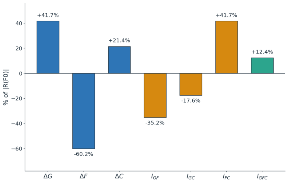
Figure 5.
Sensitivity of the main effects (ΔG, ΔF), the compression main effect (ΔC), and the two largest interactions (, ) to OCR (3–10; OCR=2 excluded as a degenerate case for the classical baseline, see text), Boston Blue Clay. ΔF is the largest single quantity throughout; is consistently large and comparable to the main effects over OCR=3–8 (its OCR=10 value is undefined — hardening singularity in F6, see text), while shrinks in magnitude and ΔC grows as OCR increases.
Figure 5.
Sensitivity of the main effects (ΔG, ΔF), the compression main effect (ΔC), and the two largest interactions (, ) to OCR (3–10; OCR=2 excluded as a degenerate case for the classical baseline, see text), Boston Blue Clay. ΔF is the largest single quantity throughout; is consistently large and comparable to the main effects over OCR=3–8 (its OCR=10 value is undefined — hardening singularity in F6, see text), while shrinks in magnitude and ΔC grows as OCR increases.
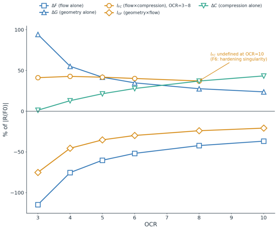
Figure 7.
Chatwong et al.’s [11] own computed model-prediction curves (orange) against real undrained triaxial test data (blue markers, compiled from [34,35,36,37] via Chatwong et al. [11]), for all four calibrated soils across their full range of tested OCR values. The dotted line q̄=p̄ marks the critical-state condition.
Figure 7.
Chatwong et al.’s [11] own computed model-prediction curves (orange) against real undrained triaxial test data (blue markers, compiled from [34,35,36,37] via Chatwong et al. [11]), for all four calibrated soils across their full range of tested OCR values. The dotted line q̄=p̄ marks the critical-state condition.
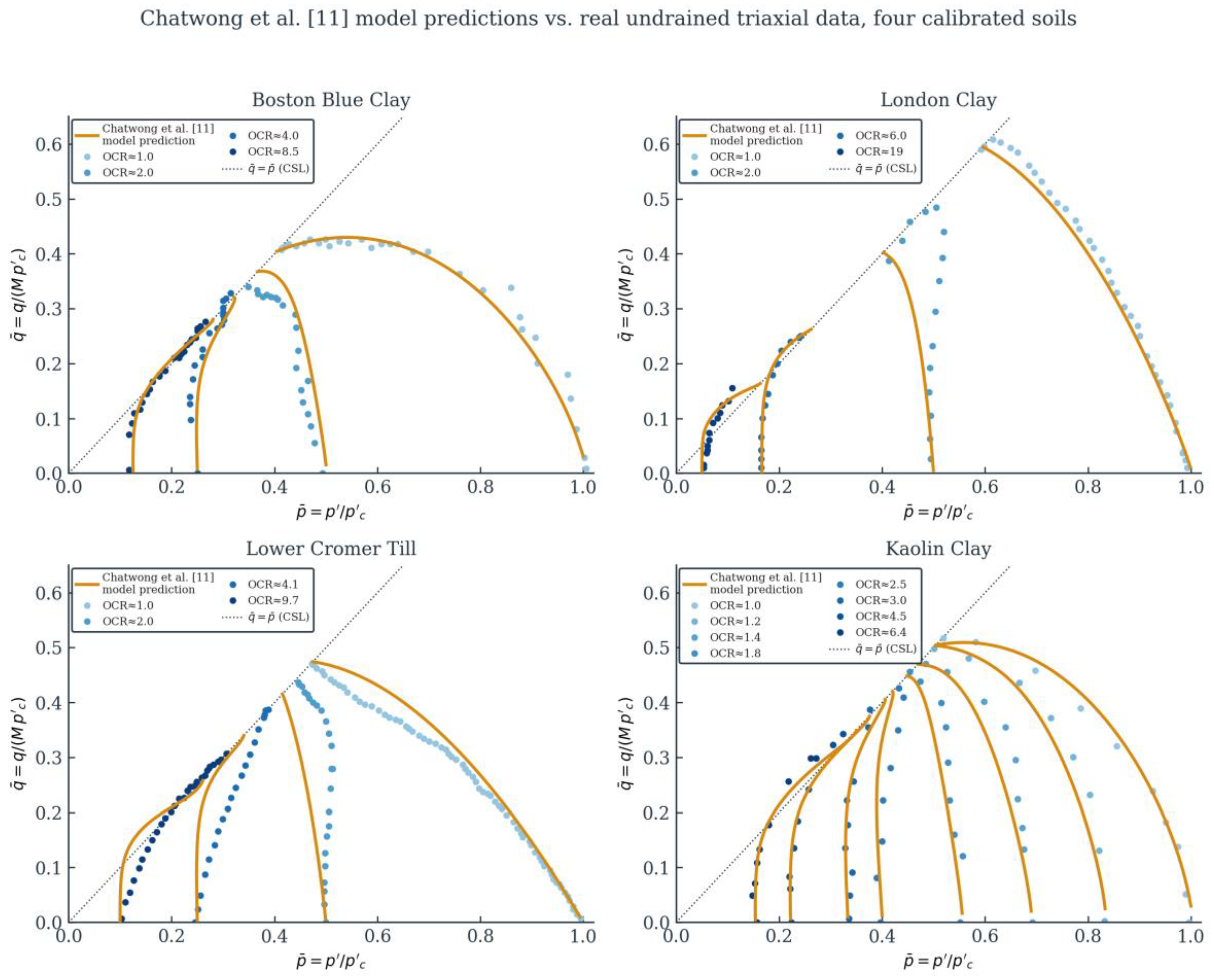
Figure 8.
Main effects (ΔG, ΔF, ΔC) and the two largest interactions (, ) at OCR=5, Boston Blue Clay, recomputed with the fractional order α held fixed across 0.3–0.9. The dotted line marks ≈0.641, the value used throughout Section 3.3 and Section 3.4. ΔG and ΔC are independent of α by construction; ΔF and are the most α-sensitive quantities.
Figure 8.
Main effects (ΔG, ΔF, ΔC) and the two largest interactions (, ) at OCR=5, Boston Blue Clay, recomputed with the fractional order α held fixed across 0.3–0.9. The dotted line marks ≈0.641, the value used throughout Section 3.3 and Section 3.4. ΔG and ΔC are independent of α by construction; ΔF and are the most α-sensitive quantities.
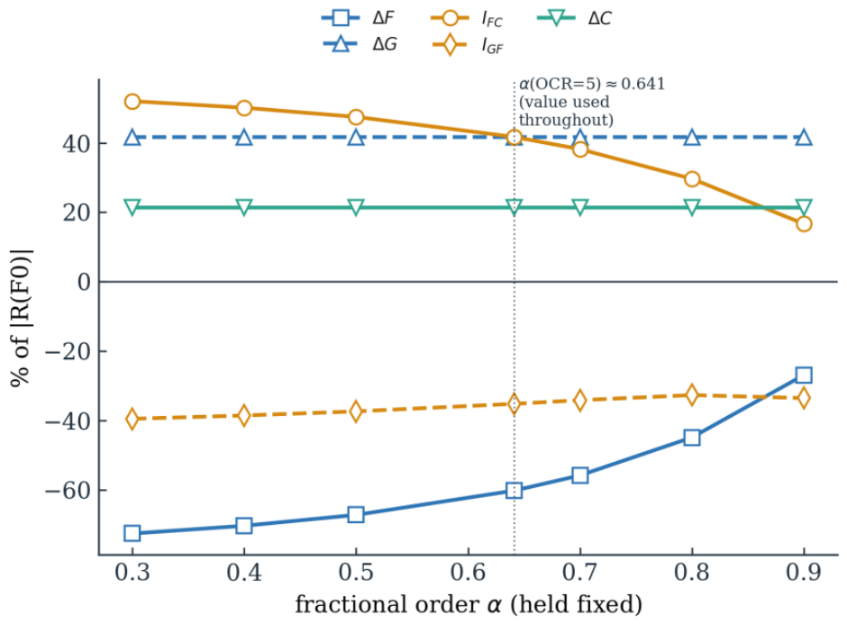
Table 1.
Constitutive components and treatment in this study.
| Component | Treatment in this study | Reason |
|---|---|---|
| Yield geometry | Modified: continuous teardrop geometry [11] | Tests whether fractional flow and hardening depend on surface geometry |
| Plastic flow | Modified: state-dependent fractional stress-gradient | Generates non-associated flow without an independent plastic potential |
| Evolution / mapping | Preserved: no mapping rule used | Avoids mixing geometry-flow-compression effects with a fourth mechanism |
| Hardening / compression law | Modified: nonlinear AJOP-based replaces constant λ [30,31] |
Tests whether a stress-dependent hardening modulus interacts with geometry and flow |
Table 2.
2×2×2 factorial constitutive assessment design.
| Framework | Yield geometry | Flow operator | Hardening / compression | Purpose |
|---|---|---|---|---|
| F0 | Classical | Integer-order | Conventional (λ) | Full baseline |
| F1 | Teardrop | Integer-order | Conventional (λ) | Geometry alone |
| F2 | Classical | Fractional | Conventional (λ) | Flow alone |
| F3 | Classical | Integer-order | AJOP () | Compression alone |
| F4 | Teardrop | Fractional | Conventional (λ) | Geometry × flow |
| F5 | Teardrop | Integer-order | AJOP () | Geometry × compression |
| F6 | Classical | Fractional | AJOP () | Flow × compression |
| F7 | Teardrop | Fractional | AJOP () | Full combined response |
Table 3.
AJOP parameters (Phonchamni et al. [31], Table 1) and derived compression moduli for three clays.
| Soil | Γ | R (kPa) | θ |
(R/2–2R secant) |
at p′=R | asymptote (high stress) | |
|---|---|---|---|---|---|---|---|
| Boston blue clay | 1.206 | 0.430 | 497 | 0.076 | 0.187 | 0.187 | 0.374 |
| London clay | 0.850 | 0.135 | 530 | 0.0058 | 0.059 | 0.059 | 0.117 |
| Bangkok clay | 2.540 | 0.700 | 59 | 0.019 | 0.304 | 0.304 | 0.608 |
Disclaimer/Publisher’s Note: The statements, opinions and data contained in all publications are solely those of the individual author(s) and contributor(s) and not of MDPI and/or the editor(s). MDPI and/or the editor(s) disclaim responsibility for any injury to people or property resulting from any ideas, methods, instructions or products referred to in the content. |
© 2026 by the authors. Licensee MDPI, Basel, Switzerland. This article is an open access article distributed under the terms and conditions of the Creative Commons Attribution (CC BY) license (http://creativecommons.org/licenses/by/4.0/).
Copyright: This open access article is published under a Creative Commons CC BY 4.0 license, which permit the free download, distribution, and reuse, provided that the author and preprint are cited in any reuse.


