

Submitted:
06 July 2026
Posted:
08 July 2026
You are already at the latest version
Abstract
The Split Delivery Vehicle Routing Problem (SDVRP) necessitates the coordination of route sequencing and order-splitting decisions, whose heterogeneous structure may constrain the efficacy of metaheuristics that update all decision variables under uniform search dynamics. This study introduces a Block-Scaled Grey Wolf Optimizer (BS-GWO) for a parameterized variant of the SDVRP, wherein order allocation and cycle time are determined in an initial stage, while the primary optimization process concentrates on operational vehicle-level splitting and route sequencing. Each candidate solution is represented by a continuous vector divided into two blocks: one associated with the visiting sequence and the other with the allocation of product units among vehicles. In contrast to the classical Grey Wolf Optimizer (GWO), the proposed BS-GWO incorporates differential block-wise scaling and maximum displacement control per block while maintaining the original α, β, and δ leadership structure. The results show that BS-GWO achieved more consistent solution quality than the classical GWO and the best overall performance among the compared metaheuristics. These findings suggest that adapting the search dynamics to the internal structure of the solution vector enhances the ability to solve heterogeneous SDVRP representations within the considered formulation.
Keywords:
grey wolf optimizer
; block-scaled grey wolf optimizer
; split delivery vehicle routing problem
; swarm intelligence
; metaheuristics
1. Introduction
Within the supply chain, logistics represents a critical subprocess that involves the procurement, handling, and distribution of products. Transportation constitutes a substantial portion of logistics costs, accounting for approximately 40–60% of total logistics expenditure and nearly 6–7% of the final product price [1]. In this context, the Vehicle Routing Problem (VRP) has become established as a fundamental model for transportation route planning, determining how a fleet of vehicles should serve a set of customers while minimizing total operating costs [2].
However, the classical VRP is based on simplified assumptions that are seldom met in real logistics systems. Consequently, the VRP has evolved into several variants designed to more accurately represent distribution systems and their practical applications [3]. One such extension is the Split Delivery Vehicle Routing Problem (SDVRP). In the classical VRP, each customer must be visited exactly once, and their demand must be fully satisfied by a single vehicle. Nevertheless, in many logistics contexts, this restriction is unnecessarily rigid. The SDVRP relaxes this condition by allowing customer demand to be split and served by different vehicles [4].
The VRP belongs to the class of NP-hard combinatorial optimization problems. Due to this nature, several exact optimization approaches have been developed to solve it, including integer linear programming formulations and algorithms based on branch-and-bound schemes. These methods can guarantee solution optimality by systematically exploring the search space [5]. However, their practical application is limited because the computational effort required increases exponentially as the number of customers grows, rendering the complete enumeration of alternatives prohibitive in real-world applications [5,6]. Furthermore, in nonlinear or multimodal problems, deterministic procedures tend to explore restricted regions of the search space, thereby reducing their efficiency [7].
In response to these limitations, research in routing optimization has increasingly focused on the development of approximate methods. In particular, metaheuristics have proven to be an effective alternative by employing stochastic and iterative search processes that enable the exploration of different regions of the solution space. These techniques use adaptive strategies and rules to obtain approximations to the optimal value within acceptable computational times, even for large-scale combinatorial problems [8]. Unlike exact methods, metaheuristics offer high flexibility for addressing optimization problems with multiple constraints, which has encouraged their application to a wide range of real-world problems in engineering, planning, and distribution [9].
Within this framework, Swarm Intelligence (SI) algorithms have gained particular relevance due to their inspiration from the collective behavior of natural systems. A representative example is Particle Swarm Optimization (PSO), in which each particle adjusts its trajectory by considering both its individual experience and the global information shared by the swarm [10]. This mechanism enables a balance between exploration of the search space and intensification around high-quality solutions, which explains why SI approaches have been widely adopted in diverse optimization problems [11].
Among SI metaheuristics, GWO was introduced as an algorithm inspired by the social hierarchy and hunting behavior of grey wolves [12,13], and it has become established as a population-based method with a relatively simple structure, facilitating its adaptation to various contexts, including binary versions and multi-objective formulations [14,15]. However, despite its acceptance, the literature has identified significant limitations when GWO encounters complex or high-dimensional search spaces. Specifically, its local search capability may be insufficient, resulting in relatively slow convergence, stagnation in local optima, and an unstable balance between exploration and exploitation [16]. Additionally, the use of its linearly decreasing convergence factor has been questioned, as it imposes a rigid transition between exploration and exploitation and does not adequately respond to the changing needs of the iterative process. Furthermore, population diversity has been observed to decrease in later stages, diminishing the algorithm’s ability to explore new regions and increasing the likelihood of convergence toward suboptimal solutions [17].
Despite GWO’s competitive performance relative to several SI-based metaheuristics, its effectiveness is not universal, as suggested by the No Free Lunch theorem. The algorithm has demonstrated competitive performance in single-objective optimization problems; however, its efficacy may diminish in multimodal, high-dimensional, or structurally complex search scenarios. The position update mechanism, primarily guided by the , , and leaders, promotes rapid exploitation of the search space, which may lead to premature convergence toward local optima. Additionally, an increase in the number of decision variables can degrade performance, especially when population diversity decreases during advanced search stages and the algorithm lacks adequate mechanisms to restore exploration after converging toward suboptimal regions. Consequently, the effective application of GWO necessitates modifications or adaptive adjustments aimed at maintaining the balance between exploration and exploitation, thereby enhancing its capability to approximate the global optimum [18].
In light of these limitations, it is pertinent to develop mechanisms that enhance exploration capacity without compromising exploitation around high-quality solutions. This study proposes a variant of the Grey Wolf Optimizer, termed the Block-Scaled Grey Wolf Optimizer (BS-GWO), designed to incorporate a differentiated treatment of the search space. Within this framework, the algorithm seeks to improve the balance between exploration and exploitation by preventing all dimensions of the solution vector from being updated under the same dynamics. Specifically, the proposed approach introduces a differentiated treatment for decision blocks with distinct operational meanings, allowing the intensity of movement to be adapted to the internal structure of the vehicle routing problem.
The principal contributions of this study are delineated as follows:
- 1.
- A variant, termed BS-GWO, is introduced, which integrates a differential movement-scaling mechanism and displacement-size control based on decision blocks. This mechanism aims to enhance the equilibrium between exploration and exploitation within heterogeneous search spaces.
- 2.
- The BS-GWO algorithm is tailored to the SDVRP through a continuous encoding scheme, organized into two heterogeneous blocks: an order block, which induces visit priority and route sequencing, and a split block, which allocates previously parameterized quantities among available vehicles.
- 3.
- A comparative experimental evaluation is performed against the classical GWO and representative state-of-the-art metaheuristics, with solution quality as the primary criterion and statistical performance analysis of the algorithms as a supplementary assessment.
- 4.
- The experimental findings show that the differentiated treatment of solution-vector blocks enhances the quality of the solutions obtained and fosters more consistent algorithmic performance in combinatorial instances of increased complexity.
The remainder of this paper is structured as follows. Section 2 reviews related work on Swarm Intelligence, GWO, and the SDVRP. Section 3 presents the problem statement, modeling assumptions, and mathematical formulation of the parameterized SDVRP. Section 4 describes the continuous encoding scheme, the normalized implementation of the classical GWO, and the proposed BS-GWO algorithm. Section 5 details the experimental design, parameter calibration, comparative results against the classical GWO and other metaheuristics, and discussion. Finally, Section 6 presents the conclusions, and Section 7 outlines future research directions.
2. Related Work
This section reviews two research streams relevant to the proposed approach: improved variants of GWO and solution strategies for SDVRP-related formulations. In response to these limitations, various variants and enhancement strategies have been developed to reinforce neighborhood search, increase learning flexibility, and stabilize convergence. A representative example is the Improved Grey Wolf Optimizer (I-GWO), which integrates the Dimension Learning-Based Hunting (DLH) strategy. This mechanism enables each wolf to update its position not only based on traditional hierarchical guidance but also through learning derived from its neighbors and additional population-level information, with the objective of improving the balance between exploration and exploitation and reducing the likelihood of stagnation in local optima [19,20]. Concurrently, variants based on distance measures and adaptive weighting functions, multiple search strategies, and enhanced update mechanisms have been proposed to mitigate premature convergence, avoid stagnation in local optima, and improve the balance between global exploration and local exploitation [21,22,23]. Similarly, Cheng and Liu [24] employ hybrid strategies and structural intensification mechanisms in route-planning problems, integrating chaotic initialization, horizontal and vertical crossover operators, Gaussian mutation, and adjustments to the leadership dynamics to reduce blind search zones and mitigate premature convergence.
Although these improvements have enhanced the performance of GWO in various contexts, a significant methodological opportunity remains concerning how the update dynamics are adapted to the internal structure of the solution vector. Firstly, it has been noted that the issue is not confined to premature convergence but also involves the rigid manner in which information from , , and is transmitted to the rest of the population, as learning concentrated on the three best individuals may restrict the utilization of alternative experiences and reduce the effective diversity of the search process [25]. Secondly, when the algorithm is applied to discrete, NP-hard problems with multiple local optima, a uniform treatment of the search space may be limited, as different parts of the decision vector may require differentiated mechanisms of exploration and refinement. This necessity has been noted in complex scheduling problems, where assignment, sequencing, and resource-selection decisions interact within the same solution representation [26]. Finally, previous studies on multi-objective problems provide precedents in which the solution representation itself may integrate heterogeneous components, such as binary variables and numerical bounds, suggesting that GWO should be adapted to the internal structure of the problem rather than operating as if all dimensions of the solution vector behaved uniformly [27].
The necessity to adapt search dynamics to non-homogeneous structures is particularly pertinent in models such as the SDVRP. This model can be viewed as an extension of the VRP and, more specifically, as a relaxation of the Capacitated Vehicle Routing Problem (CVRP). While the VRP seeks to design efficient routes to meet distributed demand using a fleet of vehicles, the CVRP introduces explicit capacity constraints, thereby increasing its complexity and classifying it among the classical combinatorial optimization problems in Operations Research [4]. Within this family, the SDVRP is characterized by relaxing the single-visit constraint, permitting a customer’s demand to be fulfilled by multiple vehicles. This feature enhances the operational flexibility of the system and may result in reductions in total cost, the number of vehicles utilized, or the distance traveled [1]. However, this same flexibility enlarges the solution space and complicates the problem’s analysis, as each customer may be associated with multiple feasible routes. Consequently, the problem becomes computationally more demanding and necessitates modeling and solution approaches that align with its structure [28,29].
Over time, the SDVRP has grown increasingly complex as additional constraints and sources of variability have been integrated into the model. In this context, specialized formulations, optimization-based heuristics, and column-generation procedures have been proposed, yielding relevant results and enhancing solution quality across various test sets. Nonetheless, exact methods have continued to exhibit notable limitations when optimally solving larger instances [30,31]. In variants with two-dimensional loading constraints, exact procedures can provide good results for small instances, but their scalability diminishes rapidly, rendering intensified local search strategies and specialized neighborhoods preferable for larger problems [32]. This trend is also evident in problems involving environmental criteria and loading constraints, where Variable Neighborhood Search (VNS) schemes with novel solution representations and operators specifically designed to maintain feasibility and search quality in more demanding spaces have been proposed [33]. Similarly, in models combining split pickup and split delivery, proposals based on Ant Colony Optimization and hybrid update mechanisms have been reported, confirming that methodological diversity increases as the structural composition of the problem becomes more complex [34].
Nevertheless, a significant portion of the recent literature on the SDVRP continues to leave unresolved a pertinent methodological issue: the explicit adaptation of search mechanisms to solution representations that encompass decisions of varying natures. In models incorporating loading incompatibility and order-based split deliveries, the solution must concurrently coordinate order compatibility, order assignment to vehicles, and route design, thereby substantially increasing the complexity of both the formulation and the solution method [35]. In scenarios where split deliveries are combined with discrete and indivisible orders, the solution representation becomes non-trivial, necessitating specific problem-reduction mechanisms and specialized encoding, thus indicating the insufficiency of a uniform strategy [36].
This challenge is exacerbated when additional location decisions, loading compatibility, and energy constraints are introduced, as the problem structure becomes heterogeneous, requiring solution mechanisms capable of coordinating interdependent sub-decisions [37]. Similarly, in variants related to omnichannel retailing, where multiple products, different types of time windows, and integer restrictions on split quantities coexist, the search process must simultaneously coordinate insertion decisions, volume assignment, and temporal feasibility. This complexity is evident in proposals such as a modified Adaptive Large Neighborhood Search (ALNS), whose repair operators consider both feasible insertion positions and the assignment of multiple products or orders under capacity and time constraints [38]. In this context, the next phase in the development of methods for the SDVRP involves not merely intensifying the search process, but explicitly adapting the search process to the differentiated structure of its variables and decisions.
3. Problem Statement and Solution Framework
The problem addressed in this study is derived from the Multi-Vendor Single-Buyer (MVSB) supply framework described by Marpaung et al. [39], in which multiple suppliers contribute to the provision of several products under capacity, transportation-cost, and route-duration constraints. However, the present research does not simultaneously solve the original integrated formulation. Instead, it focuses on a parameterized logistics execution problem in which the supplier–product allocation structure and the cycle time are determined before the route optimization stage.
3.1. Modeling Assumptions and Scope
Before describing the two-stage solution framework, it is necessary to define the modeling assumptions and scope under which the problem is addressed. First, the instances considered in this study are synthetic and are constructed in a controlled manner through combinations of suppliers, products, and vehicles. This design enables the evaluation of the algorithmic behavior under different levels of structural complexity. However, the instances are not intended to represent a specific real-world logistics system, but rather to provide a controlled experimental setting for assessing the proposed method.
Second, the problem addressed corresponds to a parameterized variant of the SDVRP. The supplier–product order allocation and the cycle time are determined before the routing optimization stage. Therefore, the main optimization process focuses on the operational splitting of predefined quantities and the construction of feasible vehicle routes. Under this assumption, BS-GWO does not simultaneously solve the complete integrated inventory, allocation, and routing model. Instead, it optimizes the logistics execution stage associated with the parameterized SDVRP formulation.
Third, the number of available vehicles, product demands, supplier capacities, vehicle capacities, setup costs, unit product weights, loading and unloading times, and distance matrix are assumed to be known for each instance. The travel time between nodes is computed from the corresponding distance under a fixed average operating speed. These assumptions allow the routing model to evaluate capacity, continuity, and route-duration feasibility in a consistent manner across all generated instances.
Finally, the calibration of BS-GWO is conducted over a discrete set of parameter levels defined through a full factorial design. Consequently, the selected configuration represents the best-performing alternative within the evaluated design space, rather than a globally optimal parameterization over a continuous parameter domain. Under these assumptions, the following subsections describe the preprocessing model and the mathematical formulation of the parameterized SDVRP.
3.2. General Solution Framework
The proposed solution framework is organized as a sequential two-stage approach. In the first stage, the order-allocation proportion associated with supplier i and product o, denoted by , as well as the cycle-time parameter T, are obtained following a decomposition logic inspired by the original MVSB formulation. Given the total demand of product o, , the target quantity to be collected from each supplier–product pair is computed as follows:
Once these quantities have been defined, is no longer treated as a decision variable in the main optimization problem. Instead, it becomes an input parameter for the routing stage. Therefore, the problem solved by the metaheuristic algorithms is not to determine the supplier-level order allocation, but to operationally execute a previously established allocation structure.
The second stage constitutes the main optimization component of the proposed method and addresses a parameterized variant of the Split Delivery Vehicle Routing Problem (SDVRP). In this stage, two interdependent decisions must be coordinated: first, the distribution of each predefined supplier–product quantity, , among the available vehicles; and second, the sequencing of supplier visits within feasible vehicle routes. For this purpose, each candidate solution is represented by a continuous vector divided into two heterogeneous decision blocks. The first block controls the visit-priority values used for route construction, whereas the second block regulates the distribution of the quantities among the available vehicles. Based on this representation, the classical GWO, the proposed BS-GWO, and the comparative metaheuristic algorithms are applied under the same encoding, decoding, and evaluation structure. Each candidate solution is decoded into vehicle routes, its operational feasibility is assessed with respect to capacity, route-continuity, and maximum-duration constraints, and its total collection cost is computed using a penalized fitness function.
Accordingly, BS-GWO does not directly solve the original integrated MVSB formulation. Rather, it optimizes the logistics execution stage associated with a parameterized SDVRP instance. Figure 1 summarizes the sequential structure of the proposed solution framework.
3.3. Preprocessing Stage: Order Allocation Model and Cycle Time
From an operational perspective, this stage receives as input the demand by product, supplier capacity, setup costs associated with product preparation, vehicle capacity, and unit weight by product. Based on this information, a model is constructed whose purpose is to determine the proportion of the total demand of product o that must be served by supplier i. Table 1 summarizes the notation used in this stage.
Order allocation is determined through a model designed to distribute the total demand of each product o among the suppliers i. The model’s function is to derive a feasible matrix that aligns with the availability constraints of each supplier. In accordance with the logic of the base model [39], the auxiliary objective function employed to obtain the allocation matrix can be expressed as follows:
In practical terms, the optimization of facilitates the derivation of a product-level allocation pattern that is compatible with the relative capacity of the suppliers and the inventory–collection coordination reported in the reference literature, subject to the following constraints.
- Total coverage constraint by product.
Once the matrix has been obtained, the subsequent step involves calculating the cycle time T according to the problem parameters [39]. Within the reference theoretical framework, this variable serves as a global link connecting product supply with the logistics execution performed by the vehicles. The cycle time associated with a configuration using R vehicles is defined as follows:
where represents the total annual demand expressed in weight units.
3.4. Mathematical Formulation of the SDVRP Model
Upon determining the order allocation coefficients and the operational cycle time T during the preprocessing stage, the primary routing instance is established. In this phase, the base supplier–product allocation is no longer treated as a decision variable but as a predetermined parameter, specifying the target quantity to be collected from each supplier i and product o during the specified cycle. Consequently, the main stage of the model is formulated as a variant of the SDVRP, which aims to optimize the splitting of the quantities , previously defined in Equation (1), among available vehicles and the sequencing of routes to minimize total collection costs. The notation used in this stage is summarized in Table 2.
These quantities serve as the quantitative link between the preprocessing stage and the main optimization stage. From this juncture, the base allocation is no longer a decision variable but becomes part of the input data for the vehicle routing problem. Similarly, the travel time between nodes is calculated as follows:
This expression assumes an average operating speed of 40 km/h [39]. Consequently, the primary problem no longer involves deciding the purchase quantities from each supplier but focuses on the logistical execution of the predetermined quantities, adhering to constraints of capacity, flow continuity, route duration, and subtour elimination.
- Objective function.
The total system cost is defined as the sum of the fixed cost associated with vehicle activation and the variable cost associated with the distance traveled by each route. Since the model operates over a cycle time T, the cost is expressed in annualized form as follows:
Routing constraints.
The routing constraints ensure flow continuity in each route, proper connection with the depot, and that each vehicle visits each supplier at most once.
- Flow conservation constraint. This constraint ensures that if a vehicle visits a supplier, it must also leave that supplier.
These constraints link the collected quantities with the visit structure and ensure that the target quantities , defined in Equation (1), are fully covered during the cycle.
- Quantity satisfaction per cycle. This constraint guarantees that the predefined quantity for each supplier–product pair is covered by the sum of the quantities collected by all vehicles.
The following constraints model the evolution of the load along each route and limit the total capacity of each vehicle.
- Cumulative load. This constraint represents the load of product o in vehicle v when moving from node i to node j, and it is activated only when arc is traveled.
To avoid cycles disconnected from the depot, a vehicle-level subtour elimination constraint is used. These constraints prevent the formation of internal cycles that are not connected to the depot.
Route-duration limit.
The total time consumed by each route must be compatible with the cycle time T. The first term of the inequality represents the total travel time, while the second incorporates the service time at the visited suppliers. The right-hand side limits the total route duration according to the previously fixed cycle.
Variable domains.
Finally, the domains of the variables are defined as follows:
The previous formulation represents the target problem of the second stage of the proposed framework. The model is addressed through a continuous representation, a metaheuristic decoding procedure, and a penalized evaluation function, which are described in the following subsections.
4. GWO and BS-GWO Implementation
To address the SDVRP variant using population-based metaheuristics, the primary phase of the problem is represented through a continuous decision vector. This representation does not directly model the binary and continuous variables of the target mathematical formulation. Instead, it establishes a compact encoding from which these decisions are subsequently reconstructed via a decoding procedure. The necessity for this representation arises from the problem’s combination of two distinct types of decisions: the sequencing of vehicle visits and the splitting of the quantities among the available vehicles. Consequently, the search space is not treated as homogeneous but is divided into blocks with distinct operational meanings.
Let be the set of suppliers, the set of vehicles, and the set of products. Then, the continuous vector of a candidate solution is defined as follows:
where represents the sequencing or order block, and represents the splitting block. The total dimension of the vector is given by:
A total of components is used for the splitting block because the proportion assigned to the last vehicle is obtained as a residual value, ensuring that the sum of fractions for each supplier–product pair is equal to one. The complete encoding can be interpreted as a two-level mechanism. The splitting block determines the participation of each vehicle in serving the quantities , whereas the order block establishes the relative priority with which the served suppliers are inserted into the route of each vehicle. Under this structure, the continuous solution does not directly represent a feasible route in terms of arcs, but rather a compact description of:
- 1.
- The quantity of product o served by each vehicle v from supplier i.
- 2.
- The relative priority of each supplier within the route associated with that vehicle.
Therefore, the solution vector is organized into heterogeneous blocks rather than as a uniform encoding for all dimensions. The encoding defined in this section constitutes the basis on which both the classical GWO and the proposed BS-GWO algorithm operate.
4.1. Base Implementation of GWO
To establish a direct methodological benchmark for assessing the impact of the proposed modification, this study employed a normalized implementation of the classical Grey Wolf Optimizer as the baseline comparison algorithm. Originally introduced by Mirjalili et al. [12], GWO is a population-based metaheuristic inspired by the social hierarchy and hunting behavior of grey wolves. Within this framework, the population is structured into four hierarchical levels: , , , and . The best solution found is identified as , while the second- and third-best solutions are designated as and , respectively, with the remaining individuals classified as . The search dynamics are directed by these three leaders, enabling the rest of the population to update their positions based on their relative locations.
In the original formulation, the encircling behavior of the prey is modeled through the following equations:
where represents the current position of a wolf, denotes the estimated position of the prey, and and are random coefficient vectors. These vectors are computed as follows:
where and are random vectors uniformly distributed in , while the parameter a decreases linearly from 2 to 0 throughout the iterations. Under this framework, GWO integrates exploration and exploitation through the behavior of : when , individuals tend to diverge from the estimated target, promoting exploration; when , movements concentrate around the best solutions, enhancing exploitation.
Since the exact position of the prey is unknown in a real optimization problem, the classical GWO assumes that the three best individuals in the population provide the best available estimate of this location. Consequently, for each individual, three displacement vectors are computed with respect to , , and :
The three candidate positions induced by the leaders are then obtained as follows:
The new position of the individual is then obtained as the average of these three estimates:
This mechanism constitutes the central update rule of the classical GWO and represents the coordinated hunting behavior of the pack around the estimated prey.
In the implementation adopted in this study, the classical GWO was used as a direct baseline to solve the parameterized SDVRP variant described in the previous sections. To this end, the algorithm was adapted to the continuous search space of the problem through a normalized representation:
where d is the total dimension of the decision vector. The correspondence between the normalized space and the real problem space is established through the following mapping:
where and represent the lower- and upper-bound vectors of the instance, respectively. Thus, the initial population is randomly generated within the unit hypercube, and each individual is transformed into the real search space before being evaluated by the fitness function. After each update, the positions are bounded again within the interval to preserve the consistency of the representation.
The computational procedure adheres to the conventional framework of GWO. Initially, a random initial population is generated, and each individual is assessed using the penalized objective function pertinent to the problem. Subsequently, the three best individuals within the population are identified and assigned to the , , and hierarchies. In each iteration, the parameter a is updated linearly, the random coefficients , , , , , and are generated, and the new position of each individual is calculated through the averaging rule based on the estimates of the three leaders. Upon obtaining the new population, each individual is re-evaluated, and the three global leaders are updated accordingly. This iterative process continues until the maximum number of iterations, defined as the stopping criterion, is achieved.
From a methodological standpoint, this version of GWO is pivotal in the comparative study because it retains the core update logic of the classical GWO and shares the same experimental framework with the BS-GWO, including the continuous representation, search bounds, evaluation function, stopping criterion, and problem instances.
4.2. Proposed BS-GWO Algorithm
While the classical GWO serves as a competitive and conceptually straightforward baseline, its update rule applies a uniform dynamic across all dimensions of the solution vector. This characteristic is limiting for the problem addressed in this study, as the continuous solution comprises blocks with distinct operational meanings: an order block, associated with vehicle-level visit priority, and a splitting block, associated with the distribution of quantities among the available fleet. Given that these blocks represent decisions of different natures, it is unreasonable to assume they should evolve with identical movement intensity within the search space. In light of this observation, BS-GWO is proposed. Its primary contribution lies in introducing block-wise differential scaling and a maximum displacement limit per block into the standard GWO dynamics.
It is important to emphasize that BS-GWO does not alter the leadership hierarchy of the classical GWO. The , , and solutions remain defined as the three best individuals in the population, and the new position of each wolf continues to be calculated from the average of three leader-based estimates. The proposed modification is introduced in the displacement intensity, such that the movement induced by , , and is no longer homogeneous across all dimensions of the vector , but instead depends on the block to which each component belongs.
4.2.1. Block-Wise Differential Scaling
Let be the normalized representation of an individual, where d is the total dimension of the decision vector. As defined in Equation (29), the vector is divided into two subsets of dimensions: , corresponding to the sequencing or order block, and , corresponding to the splitting block.
Based on this partition, BS-GWO defines a dimension-wise scaling vector:
Its components are constructed as follows:
In this context, and denote block-specific scaling factors for the order block and the splitting block, respectively. Operationally, this vector modulates the displacement amplitude experienced by each dimension during the population update. Consequently, when , the dimensions associated with sequencing and those associated with load splitting evolve with varying intensities within the same iteration.
With this modification, the movement coefficients of the classical GWO are redefined as follows:
Consequently, the update of the three leader-based estimates in the normalized space is given by:
The leader-based candidate positions are then computed as follows:
A tentative average position is then obtained as:
Up to this point, the structure of the GWO is preserved, albeit with a relevant modification: the magnitude of the movement induced by the leaders depends on the decision block to which each dimension belongs.
4.2.2. Maximum Block-Wise Displacement Limit
In addition to differential scaling, BS-GWO incorporates a second mechanism: a maximum displacement limit per block, whose purpose is to prevent excessive movements within a single iteration and to control the stability of the search process. To this end, a dimension-wise maximum displacement vector is defined as:
Its components are constructed as follows:
Here, and represent the maximum displacement fractions allowed for the dimensions of the order and splitting blocks, respectively. In the implementation, these values are interpreted directly in the normalized space , so that they limit the maximum component-wise change allowed at each iteration.
Once the tentative position has been obtained, the displacement is computed as:
This displacement is then clipped component by component as follows:
Finally, the updated position of the individual is obtained as:
where denotes the component-wise bounding operation to the interval .
This mechanism serves a dual function. On the one hand, it prevents excessive oscillations or abrupt jumps in the search space. On the other hand, it allows each block to preserve a movement scale consistent with its operational role within the problem. In particular, displacement clipping is useful when certain dimensions require more controlled refinement than others, as occurs in the coordination between sequencing and splitting decisions.
4.2.3. Computational Procedure of BS-GWO
Each individual is transformed back into the real problem space using Equation (39). Then, at each iteration, the scalar parameter a is linearly updated, the vectors , , and , already scaled by blocks, are constructed, and the vectors , , and are generated in their standard form. Using these coefficients, the tentative average position is computed, the displacement is obtained, this displacement is clipped according to the vector , and the position is finally updated in the normalized space. Once the population has been updated, each individual is re-evaluated and the leader hierarchy is updated. This process is repeated until the maximum number of iterations is reached.
Based on the mechanisms described above, the complete computational procedure of BS-GWO is presented in Figure 2.
The BS-GWO algorithm retains the fundamental structure of the classical GWO, which is guided by the three best search agents. However, the position update mechanism includes two additional operations: movement scaling based on the decision block and clipping of the maximum permissible component-wise displacement. These operations enable the search process to avoid uniformly treating all dimensions of the solution vector, thereby allowing the movement intensity to be adapted according to the operational function of each block.
4.2.4. Methodological Interpretation of the Proposed Approach
From a methodological standpoint, BS-GWO can be conceptualized as an extension of the classical GWO, wherein the movement rule no longer treats all solution dimensions as structurally equivalent. While the baseline GWO applies a uniform update scheme to the entire vector , BS-GWO acknowledges that the problem under study comprises blocks with distinct functions within the decision-making process: the order block influences route sequencing, whereas the splitting block affects the operational distribution of quantities among vehicles. Consequently, the proposed algorithm adjusts both the movement scale and the maximum allowable displacement according to the respective block. This modification does not alter the fundamental nature of GWO as an algorithm guided by , , and . However, it does modify the manner in which information from these leaders is translated into effective displacements across the population. Therefore, the methodological contribution of BS-GWO lies not in redefining the leadership scheme, but in adapting the movement intensity to the internal structure of the solution vector.
5. Experiments and Results
In the absence of a publicly available benchmark in the literature that simultaneously represents the characteristics required by the studied variant—namely, multiple suppliers, multiple products, operational splitting among vehicles, capacity constraints, and route-duration limits—a synthetic set of controlled instances was constructed for experimental evaluation. This approach aligns with the reference studies on the MVSB framework, wherein small-scale numerical examples were initially employed to validate the formulation based on Marpaung et al. [40], followed by the use of synthetic parameter sets to assess algorithmic performance across varying problem scales. The experimental set comprised 48 instances, generated through the combination of three structural factors: four levels for the number of suppliers (10, 30, 50, and 70), four levels for the number of products (5, 10, 20, and 30), and three levels for the available fleet size (1, 2, and 3). This construction facilitated a gradual progression of complexity, spanning from relatively compact scenarios to larger-scale instances, while maintaining a consistent generation logic across all classes.
Each instance was generated in MATLAB via a synthetic procedure based on uniform distributions. The generation ranges were scaled according to the supplier-size class, using the small scenarios reported in the reference literature as a baseline. Under this framework, parameter scaling across classes was designed to preserve the structural consistency of the problem as the number of suppliers and products increased. For each instance, 30 independent runs were conducted, recording the objective function as the primary performance variable and execution time as a supplementary metric.
The evaluation was executed in three stages. The first stage involved identifying the best parameter combination for the BS-GWO algorithm through a full two-level factorial design, encompassing six factors and resulting in 64 combinations. The second stage entailed a comparison of the calibrated BS-GWO against the classical GWO on the 48 previously described instances using the nonparametric Wilcoxon test. The third stage extended the comparison to a set of five metaheuristics, where the overall performance was analyzed using the Relative Performance Difference (RPD), average ranks, and the Friedman and Iman–Davenport global tests.
Given the involvement of stochastic algorithms in this research, the analysis was underpinned by nonparametric tests, such as the Wilcoxon signed-rank test, alongside multiple-comparison procedures, including the Friedman test and its extensions [41]. This section is structured into four parts. Section 5.1 elucidates the parameter tuning process of BS-GWO. Section 5.2 provides a direct comparison between BS-GWO and the classical GWO, taking into account both the objective function and execution time. Section 5.3 offers a final comparison against other metaheuristics using the Relative Performance Difference (RPD), average ranks, and the Friedman and Iman–Davenport tests. Lastly, Section 5.4 synthesizes the principal findings from an integrative discussion perspective.
5.1. Parameter Calibration of BS-GWO
Prior to comparing BS-GWO with the classical GWO and other metaheuristic algorithms, a preliminary parameter-tuning phase was undertaken. For this purpose, a full factorial design was employed, comprising six factors evaluated at both low and high levels, as detailed in Table 3. This configuration resulted in 64 parameter combinations, each of which was executed through 30 independent runs for each supplier-size level.
The structure delineated above aligns with the principles of factorial designs as articulated by Adenso-Díaz and Laguna [42]. Initially, factors deemed to influence the system response are identified; subsequently, critical levels for each factor are established; and ultimately, their combinations are assessed. In the context of metaheuristics with stochastic components, these authors further observe that replications per treatment may be necessary to gather meaningful information, owing to the intrinsic variability of their search mechanisms. Montero et al. [43] explicitly highlight that the stochastic nature of metaheuristics necessitates multiple executions during the calibration of a configuration, as identical parameterizations may yield varying performance outcomes under different random seeds.
5.1.1. Evaluation Criterion and Selection Rule
In this study, calibration was not conducted using a raw global average of the objective function across all instances, as such a criterion would have introduced considerable bias. The magnitude of the objective function increases substantially with the number of suppliers; thus, larger instances would have disproportionately influenced the selection process if all results were aggregated on a single scale. To mitigate this issue, configurations were evaluated separately within four groups, categorized by the number of suppliers: 10, 30, 50, and 70. Within each group, the 64 configurations were ranked from the lowest to the highest average objective function value, thereby establishing an internal ranking for each instance family. Subsequently, for each configuration, the average of its positions across the four rankings was calculated. An aggregated ranking was then constructed from this average rank, and the configuration with the lowest value was selected as the final configuration. This approach aligns with the general principles of tuning as described in the literature. Montero et al. [43] note that the best configurations often depend on the specific problem or set of instances considered, and that the quality of a configuration should be assessed over a training set rather than isolated results. Similarly, Adenso-Díaz and Laguna [42] contend that systematic calibration should be guided by an explicit performance measure and a set of reference problems, precisely to avoid decisions that lack generalizability.
5.1.2. Best-Ranked Configurations
Table 4 delineates the ten highest-ranked configurations based on the average rank achieved across four distinct supplier-size categories. The configuration ultimately selected was No. 49, comprising 500 individuals, 1000 iterations, , , , and . This particular configuration attained rankings of 5th, 3rd, 6th, and 2nd within the groups containing 10, 30, 50, and 70 suppliers, respectively, resulting in an average rank of 4.00, the lowest among all configurations evaluated.
5.1.3. Interpretation of the Parameter Selection
The ranking presented in Table 4 facilitates the identification of pertinent patterns in the parametric behavior of BS-GWO. Firstly, 1000 iterations are consistently present in all ten best-ranked configurations, suggesting that, within the evaluated ranges, an increased search budget contributed to the stabilization of solution quality. Secondly, a discernible trend is evident for , which appears in 9 of the 10 best-ranked configurations, suggesting that the block associated with quantity splitting benefited from a more conservative search dynamic. The third pattern is observed in and , where the value 0.1 predominated among the top-ranked configurations, suggesting that more controlled movements favored the algorithm’s stability. In contrast, the behavior of did not exhibit such pronounced dominance, as the best-ranked configurations were distributed between 0.3 and 1.5. This behavior aligns with the central premise of the proposed method: a block-based representation does not necessarily respond uniformly to identical search parameters.
The selection of configuration No. 49, as opposed to another configuration with superior individual positions in certain groups, is directly related to the rank-averaging criterion employed in the final selection. The rationale is straightforward: ranking configurations first within each group and subsequently averaging their positions enables the evaluation of which configuration consistently maintains high performance across instance families of varying sizes. For instance, configuration No. 57 ranked 1st, 2nd, and 3rd in the groups with 10, 30, and 50 suppliers, respectively, but declined to 12th position in the group with 70 suppliers. In contrast, configuration No. 49 sustained high and balanced performance across all four groups, without abrupt declines. Therefore, it best represented the objective of this stage: to select a robust configuration for the entire experimental benchmark, rather than a combination that excelled only in a subset of it.
5.2. Comparison between BS-GWO and Classical GWO
Following the determination of the parametric configuration of BS-GWO, a direct comparison with the classical GWO was performed across the 48 instances of the experimental benchmark. Each algorithm was executed independently 30 times per instance. The comparison employed two metrics: the objective function, serving as the primary criterion for solution quality, and execution time, analyzed as a supplementary criterion. This approach enabled an assessment of whether the enhancement in solution quality achieved by BS-GWO was accompanied by a relevant computational penalty.
The difference between BS-GWO and the classical GWO was evaluated using the Wilcoxon test at a significance level of . The overall results of this comparison are presented in Table 5, which concurrently reports the outcomes related to the objective function and execution time.
As illustrated in Table 5, the BS-GWO algorithm achieved superior objective-function values in 33 out of 48 instances, whereas the classical GWO demonstrated superiority in 15 instances. Furthermore, 30 of the BS-GWO victories were statistically significant, compared to only 5 significant victories for the classical GWO. In contrast, execution time did not exhibit a conclusive difference. Although the classical GWO recorded lower average execution times in 29 instances, the statistically significant differences were evenly distributed, with 8 cases favoring BS-GWO and 8 favoring the classical GWO. Consequently, execution time did not distinctly differentiate the two algorithms. The primary advantage of BS-GWO was observed in solution quality, without sufficient evidence to assert a dominant computational penalty compared to the classical GWO.
5.2.1. Effect of Complexity by Instance Group
The most noteworthy outcome of this comparison is not only that BS-GWO accumulated more victories, but also the manner in which these victories were distributed as the structural complexity of the problem increased. Jamil and Yang [44] emphasize that a test set should not only be comprehensive but also sufficiently diverse to reveal the types of problems in which an algorithm truly demonstrates advantages. From this perspective, the benchmark employed in this study enabled the observation that the gains achieved by BS-GWO were not uniform but became increasingly pronounced as certain structural dimensions of the problem increased.
When the results were categorized by the number of vehicles, the pattern was particularly evident. In instances with 1 vehicle, BS-GWO outperformed the classical GWO in only 4 out of 16 cases. In contrast, with 2 vehicles, it prevailed in 13 out of 16 instances, and with 3 vehicles, it succeeded in all 16 instances. This transition is significant; it suggests that the proposed modification becomes more advantageous precisely when the problem structure exhibits greater complexity, as depicted in Figure 3.
The observed trend persisted when the results were categorized by the number of suppliers: in instances with 10 suppliers, BS-GWO surpassed the classical GWO in 5 out of 12 instances; with 30 suppliers, it prevailed in 8 out of 12; with 50 suppliers, it succeeded in 9 out of 12; and with 70 suppliers, it outperformed it in 11 out of 12. Consequently, the superiority of BS-GWO became increasingly apparent as the logistics network increased in size and, with it, the structural difficulty of the problem, as illustrated in Figure 4.
The preceding figures align with the rationale underlying the proposed method. Given that BS-GWO was designed to adapt search dynamics according to decision blocks, it is logical that its advantages are not as evident in simpler instances as they are in scenarios where the interaction among parameterized allocation, operational splitting, and routing becomes more intricate. In this context, the results suggest that the modification introduced into the GWO leadership dynamics responds better to heterogeneous and structurally more demanding search spaces.
Overall, the direct comparison with the classical GWO yields three primary conclusions. First, BS-GWO provides a real and repeatable improvement in solution quality. Second, this enhancement is not uniformly distributed across the entire experimental benchmark but tends to become more pronounced as the structural complexity of the problem increases, particularly concerning the number of suppliers and vehicles. Third, although execution time did not nominally favor BS-GWO, the time difference between the two algorithms was statistically inconclusive; thus, no relevant computational penalty can be attributed to the proposed method compared to its baseline version.
5.3. Comparison of BS-GWO against Other Metaheuristics
Following the assessment of BS-GWO’s performance against the classical GWO, a final comparison was conducted with four Swarm Intelligence metaheuristics: Particle Swarm Optimization (PSO), Ant Colony Optimization (ACO), Whale Optimization Algorithm (WOA), and Marine Predators Algorithm (MPA). These algorithms were selected to contrast the proposed method with representative approaches based on diverse search mechanisms. PSO was included due to its widespread use in population-based algorithms for continuous and combinatorial optimization; ACO was considered for its historical association with routing problems and incremental solution construction; WOA was included as a contemporary bio-inspired metaheuristic based on exploration and exploitation mechanisms; and MPA was considered for its competitive performance reported in complex optimization problems. Thus, the final comparison extended beyond evaluating BS-GWO against its baseline version, positioning it against both established and more recent methods within the SI field.
For this phase, performance was evaluated on the 48 instances of the experimental benchmark, with 30 independent runs per algorithm and instance. Table 6 presents the average objective-function value obtained by each metaheuristic for each instance. As the problem was formulated as a minimization problem, lower values indicate superior solutions; therefore, the algorithm with the best performance for each instance is highlighted in bold in each row. This table provides an initial direct reading of the comparison, illustrating the cases in which BS-GWO achieved the best average solution and the scenarios in which other algorithms yielded superior results.
In light of these findings, and given the varying scales of the objective function across instances, a direct global comparison using absolute values was deemed inappropriate. Instead, the Relative Performance Difference (RPD) metric was employed. This metric normalizes the performance of each algorithm relative to the best value found for each instance, thereby mitigating the influence of larger-scale instances on the overall statistical analysis. Following the RPD formulation used by Montiel-Arrieta et al. [7], the metric was computed as:
where denotes the Best Obtained Value by a specific algorithm for a given instance, and represents the Best Known Value found among all algorithms for that same instance. Consequently, lower RPD values signify superior relative performance. The RPD matrix served as the basis for the Friedman analysis and the Iman–Davenport statistic. Additionally, the average RPD per algorithm was calculated from this matrix and used as a global descriptive indicator of objective-function performance. Table 7 displays the average RPD for each algorithm along with its corresponding ranking in comparison to the other metaheuristics.
Global statistical analyses confirmed that the differences observed among the algorithms are not attributable to random variation. Specifically, a Friedman statistic of and an Iman–Davenport statistic of were obtained, both with . As noted by Derrac et al. [41], these findings support the presence of statistically significant global differences among the algorithms.
5.3.1. Wilcoxon Test
In addition to the global RPD-based analysis, the Wilcoxon test was employed to assess the pairwise performance of BS-GWO against each competing algorithm. This approach facilitated a more nuanced interpretation of BS-GWO’s performance relative to each competitor. Based on the average objective-function values reported in Table 6, and considering ties in the best value per instance, BS-GWO appeared as the best-performing algorithm in 28 instances, MPA in 18 instances, ACO in 4 instances, WOA in 2 instances, and PSO in 1 instance. These counts exceed 48 because ties occurred in instances 1, 7, and 10. The best-value appearances count all algorithms tied for the lowest average objective-function value in an instance. Ties occurred in instance 1 among ACO, MPA, and WOA; in instance 7 between ACO and MPA; and in instance 10 among ACO, MPA, and WOA. The columns “BS-GWO Better”, “BS-GWO Worse”, and “BS-GWO Equal” summarize the pairwise Wilcoxon-based comparison between BS-GWO and each competing algorithm across the 48 instances.
Table 8 illustrates a distinct advantage of BS-GWO over WOA and ACO, a moderate advantage over PSO, and a notably closer competition against MPA. The best-value appearance count confirms that BS-GWO achieved the largest number of best average objective-function values, even after explicitly accounting for tied cases. Consequently, while the Wilcoxon comparisons do not substitute the global Friedman test, they offer an additional perspective to discern which competitor posed the greatest challenge to the proposed method.
5.4. Discussion
The results obtained support the interpretation that the performance of BS-GWO is not contingent upon an isolated improvement in a single stage of the study, but rather on a sequence of experimental evidence. Initially, the parameter-tuning stage facilitated the establishment of a robust algorithm configuration through a full factorial design evaluated with multiple independent runs. This stage was relevant as it mitigated the risk that subsequent comparisons would rely on an arbitrary parameter combination or an exceptionally favorable run. Subsequently, the direct comparison with the classical GWO demonstrated that BS-GWO achieved superior objective-function values in most evaluated instances, with a considerable number of statistically significant differences favoring it. This evidence supports the interpretation that the proposed modification resulted not only in a numerical improvement but also in a statistically consistent advantage.
A particularly noteworthy aspect was that the advantage of BS-GWO was not uniformly distributed across the entire experimental benchmark. The results, categorized by the number of vehicles and suppliers, indicated that the performance of the proposed algorithm became more favorable as the structural complexity of the instances increased. This trend aligns with the method’s motivation, as BS-GWO was designed to adjust the search dynamics according to decision blocks with varying behaviors. In problems where sequencing, vehicle-assignment, and quantity-splitting decisions interact, a uniform update strategy may be limited. Therefore, the superior performance observed in more complex instances suggests that block-wise differential scaling facilitated a more suitable exploration of the search space.
The final comparison against other metaheuristics reinforced this interpretation. At this stage, BS-GWO not only maintained competitive behavior but also achieved the best overall performance among the evaluated algorithms when considering different indicators: average RPD, Friedman average ranks, and the Wilcoxon comparisons. This convergence of metrics is relevant because it prevents the interpretation from relying on a single performance measure. Furthermore, the analysis revealed that the advantage of BS-GWO was more pronounced against WOA and ACO, more moderate against PSO, and closer against MPA. This nuanced interpretation is important as it avoids presenting an artificially absolute superiority and acknowledges that the proposed method led the comparative set, albeit with varying margins against each competitor.
The utilization of RPD was necessary due to the varying scales of the objective function across instances. Solely comparing absolute values could have skewed the interpretation towards instances with larger magnitudes. By normalizing performance relative to the best value found in each instance, RPD facilitated a more equitable comparison among algorithms. In this context, the results derived from the Friedman and Iman–Davenport tests, based on the RPD matrix, offered a more robust global interpretation by confirming that the observed differences among the methods were not merely attributable to random variability. Another pertinent aspect was the execution time behavior. Although the classical GWO recorded a greater number of nominal wins in this metric, the statistical evidence did not demonstrate a dominant time difference between both algorithms. Consequently, the advantage of the Block-Scaled Grey Wolf Optimizer should be primarily understood in terms of solution quality, rather than as a consistent reduction in computational time.
Overall, the analysis of the results suggests that BS-GWO is particularly useful when the problem structure necessitates the coordination of heterogeneous decisions within a unified representation. The observed improvement over the classical GWO and its competitive positioning against other metaheuristics suggest that adapting the movement intensity according to the nature of the solution-vector blocks can be an effective strategy for split-delivery routing problems.
6. Conclusions
This study introduces a variant of the Grey Wolf Optimizer, termed the Block-Scaled Grey Wolf Optimizer, designed to enhance search dynamics within an SDVRP model. The proposal is predicated on the central premise that the continuous representation of the solution vector comprises blocks with distinct operational functions, rather than homogeneous decisions. Consequently, applying uniform update intensity across all dimensions of the vector may constrain the algorithm’s capacity to explore and refine solutions in problems where sequencing, vehicle-assignment, and quantity-splitting decisions coexist.
The primary methodological contribution of BS-GWO involves the integration of block-wise differential scaling and a maximum displacement limit per block into the update rule of the classical GWO. These modifications retain the hierarchical logic of the original algorithm, based on the , , and leaders, while adjusting the translation of information from these leaders into effective movement within the search space. Thus, the algorithm preserves the structural simplicity of GWO while introducing a dynamic more attuned to the internal nature of the solution vector.
Experimental results support the relevance of this adaptation. Overall, BS-GWO showed consistent improvement in solution quality compared to the classical GWO and exhibited competitive performance against other Swarm Intelligence metaheuristics. The principal contribution of this study extends beyond merely obtaining superior solutions; it underscores the importance of considering the internal structure of the representation used in the design of metaheuristic operators. In problems such as the SDVRP, where diverse logistics decisions are encoded within a single vector, a uniform update strategy may prove inadequate. From this perspective, BS-GWO provides evidence that a block-wise differentiated movement strategy can enhance search capability and foster more stable performance in combinatorial instances of greater complexity.
7. Future Work
In light of the aforementioned limitations, several avenues for future research can be identified. The first direction involves the validation of BS-GWO using real-world instances. Such validation would enable the assessment of whether the behavior observed in synthetic instances is consistent in scenarios involving distances, demands, operational constraints, and logistics patterns derived from actual systems.
Additionally, it would be pertinent to investigate adaptive versions of BS-GWO. In the current study, the scaling factors and maximum displacement limits per block were fixed through prior calibration. However, a logical extension would be to allow these parameters to dynamically adjust during the search process based on indicators such as population diversity, improvement rate, stagnation, or block-level complexity. This approach could enhance the balance between exploration and exploitation and reduce reliance on external calibration.
Another relevant research direction involves extending the block-wise approach to richer problem formulations. Future studies could consider heterogeneous fleets, time windows, multiple depots, environmental constraints, vehicle-type-dependent costs, uncertainty in demand or travel times, and product-compatibility constraints. In these contexts, the concept of differentially scaling movement by blocks could prove even more useful, as the solution vector would encompass decisions of a more diverse nature.
From a methodological standpoint, the next step should not be confined to testing BS-GWO on a larger number of instances but should concentrate on identifying the specific conditions under which block-wise differentiated treatment offers a real advantage over more conventional search strategies.
Author Contributions
Conceptualization, R.A.M. and I.B.V.; methodology, R.A.M, I.B.V. and J.C.S.T.M.; software, N.H.R. and J.C.S.T.M.; formal analysis, R.A.M., J.M.M. and N.H.R.; data curation, J.C.S.T.M. and J.M.M.; writing—original draft preparation, R.A.M. and I.B.V.
Funding
This research was funded by SECIHTI grant number 779937.
Data Availability Statement
Data available upon request.
Conflicts of Interest
The authors declare no conflicts of interest.
References
- Aghaabdollahian, B.; Javadi, B.; Aazami, A. An overview of vehicle routing problems: A comprehensive classification and description of types. Transp. Res. Interdiscip. Perspect. 2026, 36, 101808. [Google Scholar] [CrossRef]
- Cordeau, J.-F.; Laporte, G.; Savelsbergh, M.W.P.; Vigo, D. Vehicle routing. In Handbooks in Operations Research and Management Science; Barnhart, C., Laporte, G., Eds.; Elsevier: Amsterdam, The Netherlands, 2007; Volume 14, pp. 367–428. [Google Scholar] [CrossRef]
- Garside, A.K.; Ahmad, R.; Muhtazaruddin, M.N.B. A recent review of solution approaches for green vehicle routing problem and its variants. Oper. Res. Perspect. 2024, 12, 100303. [Google Scholar] [CrossRef]
- Toth, P.; Vigo, D. (Eds.) Vehicle Routing: Problems, Methods, and Applications, 2nd ed.; Society for Industrial and Applied Mathematics: Philadelphia, PA, USA, 2014. [Google Scholar]
- Toth, P.; Vigo, D. Branch-and-bound algorithms for the capacitated VRP. In The Vehicle Routing Problem; Toth, P., Vigo, D., Eds.; Society for Industrial and Applied Mathematics: Philadelphia, PA, USA, 2002; pp. 29–51. [Google Scholar] [CrossRef]
- Archetti, C.; Coelho, L.C.; Speranza, M.G.; Vansteenwegen, P. Beyond fifty years of vehicle routing: Insights into the history and the future. Eur. J. Oper. Res. 2026, 330, 355–372. [Google Scholar] [CrossRef]
- Montiel-Arrieta, L.J.; Barragan-Vite, I.; Seck-Tuoh-Mora, J.C.; Hernandez-Romero, N.; González-Hernández, M.; Medina-Marin, J. Minimizing the total waste in the one-dimensional cutting stock problem with the African buffalo optimization algorithm. PeerJ Comput. Sci. 2023, 9, e1728. [Google Scholar] [CrossRef] [PubMed]
- Detwal, P.K.; Agrawal, R.; Samadhiya, A.; Kumar, A. Metaheuristics in circular supply chain intelligent systems: A review of applications journey and forging a path to the future. Eng. Appl. Artif. Intell. 2023, 126, 107102. [Google Scholar] [CrossRef]
- Słowik, A.; Kwaśnicka, H. Evolutionary algorithms and their applications to engineering problems. Neural Comput. Appl. 2020, 32, 12363–12379. [Google Scholar] [CrossRef]
- Yang, X.-S. Particle swarm optimization. In Nature-Inspired Optimization Algorithms, 2nd ed.; Elsevier: Amsterdam, The Netherlands, 2021; Chapter 8. [Google Scholar] [CrossRef]
- Makhadmeh, S.N.; Al-Betar, M.A.; Abu Doush, I.; Awadallah, M.A.; Kassaymeh, S.; Mirjalili, S.; Abu Zitar, R. Recent advances in Grey Wolf Optimizer, its versions and applications: Review. IEEE Access 2024, 12, 22991–23028. [Google Scholar] [CrossRef]
- Mirjalili, S.; Mirjalili, S.M.; Lewis, A. Grey Wolf Optimizer. Adv. Eng. Softw. 2014, 69, 46–61. [Google Scholar] [CrossRef]
- Faris, H.; Aljarah, I.; Al-Betar, M.A.; Mirjalili, S. Grey wolf optimizer: A review of recent variants and applications. Neural Comput. Appl. 2018, 30, 413–435. [Google Scholar] [CrossRef]
- Emary, E.; Zawbaa, H.M.; Hassanien, A.E. Binary grey wolf optimization approaches for feature selection. Neurocomputing 2016, 172, 371–381. [Google Scholar] [CrossRef]
- Mirjalili, S.; Saremi, S.; Mirjalili, S.M.; Coelho, L.d.S. Multi-objective grey wolf optimizer: A novel algorithm for multi-criterion optimization. Expert Syst. Appl. 2016, 47, 106–119. [Google Scholar] [CrossRef]
- Preeti; Deep, K. A random walk grey wolf optimizer based on dispersion factor for feature selection on chronic disease prediction. Expert Syst. Appl. 2022, 206, 117864. [Google Scholar] [CrossRef]
- Yan, L.; Luo, S.; Qian, J.; Li, Y. Improved Grey Wolf Optimizer with adaptive and convergence enhancement mechanisms for high nonlinearity S-Box. Chaos Solitons Fractals 2026, 208, 118211. [Google Scholar] [CrossRef]
- Das, D.; Sadiq, A.S.; Mirjalili, S. Optimization Algorithms in Machine Learning: A Meta-Heuristics Perspective; Springer Nature Singapore: Singapore, 2025. [Google Scholar] [CrossRef]
- Nadimi-Shahraki, M.H.; Taghian, S.; Mirjalili, S. An improved grey wolf optimizer for solving engineering problems. Expert Syst. Appl. 2021, 166, 113917. [Google Scholar] [CrossRef]
- Mohammadi, S.; Nadimi-Shahraki, M.H.; Beheshti, Z. An effective Fuzzy Sign-aware Influence Maximization method in complex networks using an adaptive Improved Grey Wolf Optimizer with dynamic user interactions. Chaos Solitons Fractals 2026, 206, 117912. [Google Scholar] [CrossRef]
- Yan, F.; Xu, X.; Xu, J. Grey wolf optimizer with a novel weighted distance for global optimization. IEEE Access 2020, 8, 120173–120197. [Google Scholar] [CrossRef]
- Li, H.; Lv, T.; Shui, Y.; Zhang, J.; Zhang, H.; Zhao, H.; Ma, S. An improved grey wolf optimizer with weighting functions and its application to unmanned aerial vehicles path planning. Comput. Electr. Eng. 2023, 111, 108893. [Google Scholar] [CrossRef]
- Yu, M.; Xu, J.; Liang, W.; Qiu, Y.; Bao, S.; Tang, L. Improved multi-strategy adaptive grey wolf optimization for practical engineering applications and high-dimensional problem solving. Artif. Intell. Rev. 2024, 57, 277. [Google Scholar] [CrossRef]
- Cheng, G.; Liu, Y. Hybrid optimization algorithm for solving path planning problems based on grey wolf optimization algorithm. Sci. Rep. 2026, 16, 8479. [Google Scholar] [CrossRef] [PubMed]
- Zhang, J.; Dai, Y.; Shi, Q. An improved grey wolf optimization algorithm based on scale-free network topology. Heliyon 2024, 10, e35958. [Google Scholar] [CrossRef] [PubMed]
- Li, X.; Ma, Y.; Wu, R.; Tang, H.; Li, Y. Green fuzzy scheduling approach of hydraulic cylinder manufacturing workshop based on nonlinear grey wolf optimizer incorporating simulated annealing. Int. J. Prod. Econ. 2026, 295, 109982. [Google Scholar] [CrossRef]
- Yildirim, G.; Alatas, B. New adaptive intelligent grey wolf optimizer based multi-objective quantitative classification rules mining approaches. J. Ambient Intell. Humaniz. Comput. 2021, 12, 9611–9635. [Google Scholar] [CrossRef]
- Archetti, C.; Savelsbergh, M.W.P.; Speranza, M.G. Worst-case analysis for split delivery vehicle routing problems. Transp. Sci. 2006, 40, 226–234. [Google Scholar] [CrossRef]
- Kou, S.; Golden, B.; Bertazzi, L. Estimating optimal split delivery vehicle routing problem solution values. Comput. Oper. Res. 2024, 168, 106714. [Google Scholar] [CrossRef]
- Archetti, C.; Savelsbergh, M.W.P.; Speranza, M.G. An optimization-based heuristic for the split delivery vehicle routing problem. Transp. Sci. 2008, 42, 22–31. [Google Scholar] [CrossRef]
- Jin, M.; Liu, K.; Eksioglu, B. A column generation approach for the split delivery vehicle routing problem. Oper. Res. Lett. 2008, 36, 265–270. [Google Scholar] [CrossRef]
- Ji, B.; Zhou, S.; Yu, S.S.; Wu, G. An enhanced neighborhood search algorithm for solving the split delivery vehicle routing problem with two-dimensional loading constraints. Comput. Ind. Eng. 2021, 162, 107720. [Google Scholar] [CrossRef]
- Ferreira, K.M.; de Queiroz, T.A.; Munari, P.; Toledo, F.M.B. A variable neighborhood search for the green vehicle routing problem with two-dimensional loading constraints and split delivery. Eur. J. Oper. Res. 2024, 316, 597–616. [Google Scholar] [CrossRef]
- Ren, T.; Luo, T.; Jia, B.; Yang, B.; Wang, L.; Xing, L. Improved ant colony optimization for the vehicle routing problem with split pickup and split delivery. Swarm Evol. Comput. 2023, 77, 101228. [Google Scholar] [CrossRef]
- Guo, F.; Huang, Z.; Huang, W. Heuristic approaches for a vehicle routing problem with an incompatible loading constraint and splitting deliveries by order. Comput. Oper. Res. 2021, 134, 105379. [Google Scholar] [CrossRef]
- Gao, Z.; Deng, F.; Fu, Z.-H.; Lai, X.; Wu, Q. A problem reduction based memetic algorithm for the vehicle routing problem with discrete split deliveries and pickups. Comput. Oper. Res. 2025, 182, 107106. [Google Scholar] [CrossRef]
- Huang, Z.; Lou, Y.; Wang, Y.; Guo, F.; Dong, M. Robust optimization framework for the electric vehicle location-routing problem with split deliveries and incompatible loading. Swarm Evol. Comput. 2026, 100, 102270. [Google Scholar] [CrossRef]
- Li, N.; Wang, Z. Vehicle routing problem for omnichannel retailing including multiple types of time windows and products. Comput. Oper. Res. 2025, 173, 106828. [Google Scholar] [CrossRef]
- Marpaung, B.; Aribowo, W.; Suprayogi, S.; Halim, A.H. An integrated inventory and order pick-up model considering the vendor’s capacities and the vehicle trips’ duration for the MVSB system. J. Ind. Eng. Manag. 2024, 17, 650–663. [Google Scholar] [CrossRef]
- Marpaung, B.; Aribowo, W.; Suprayogi, S.; Halim, A.H. An integrated inventory and order pickup model in the MVSB system considering capacities of vendors. J. Phys. Conf. Ser. 2021, 1858, 012016. [Google Scholar] [CrossRef]
- Derrac, J.; García, S.; Molina, D.; Herrera, F. A practical tutorial on the use of nonparametric statistical tests as a methodology for comparing evolutionary and swarm intelligence algorithms. Swarm Evol. Comput. 2011, 1, 3–18. [Google Scholar] [CrossRef]
- Adenso-Díaz, B.; Laguna, M. Fine-tuning of algorithms using fractional experimental designs and local search. Oper. Res. 2006, 54, 99–114. [Google Scholar] [CrossRef]
- Montero, E.; Riff, M.-C.; Neveu, B. A beginner’s guide to tuning methods. Appl. Soft Comput. 2014, 17, 39–51. [Google Scholar] [CrossRef]
- Jamil, M.; Yang, X.-S. A literature survey of benchmark functions for global optimisation problems. Int. J. Math. Model. Numer. Optim. 2013, 4, 150–194. [Google Scholar] [CrossRef]
Figure 1.
Sequential solution framework for the parameterized SDVRP addressed in this study.
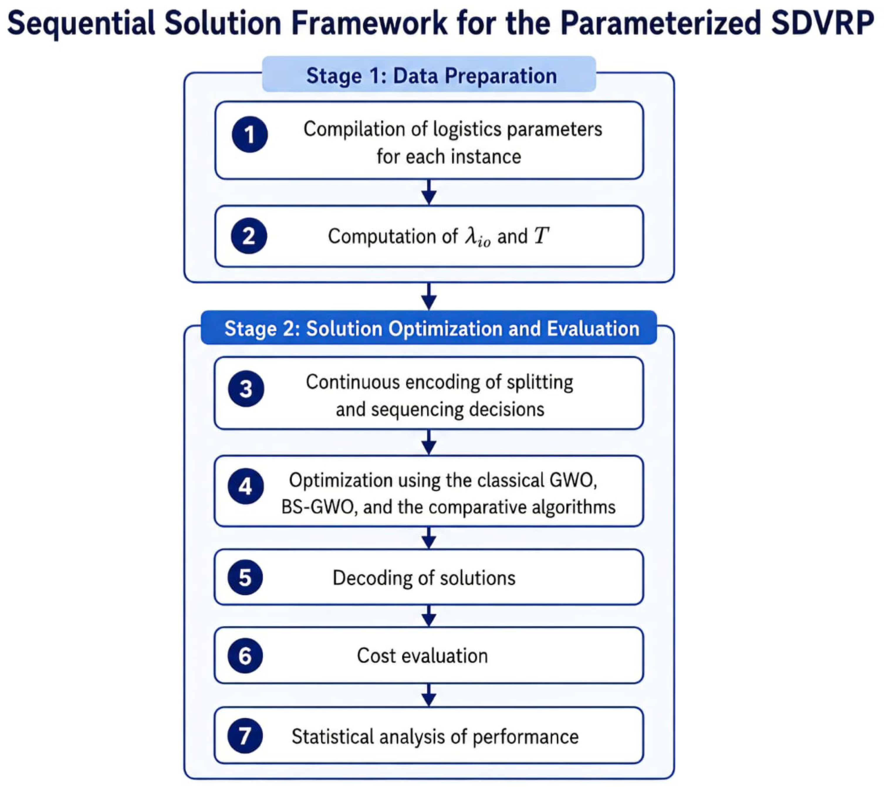
Figure 2.
Proposed Block-Scaled Grey Wolf Optimizer (BS-GWO).
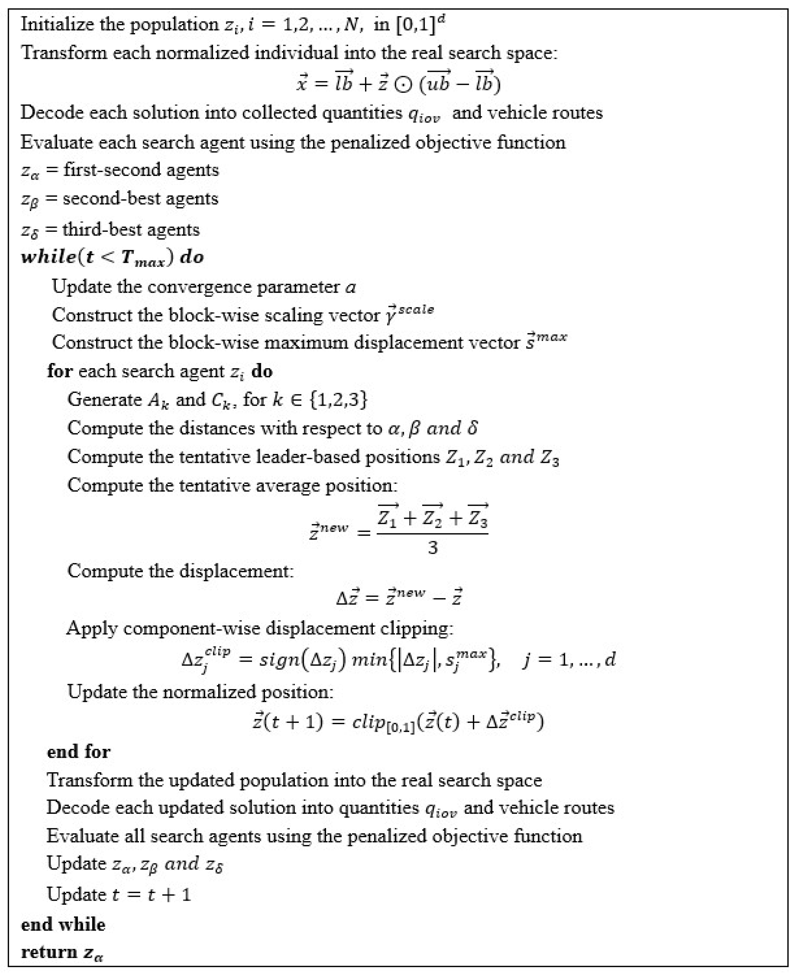
Figure 3.
Comparison between BS-GWO and classical GWO by number of vehicles.
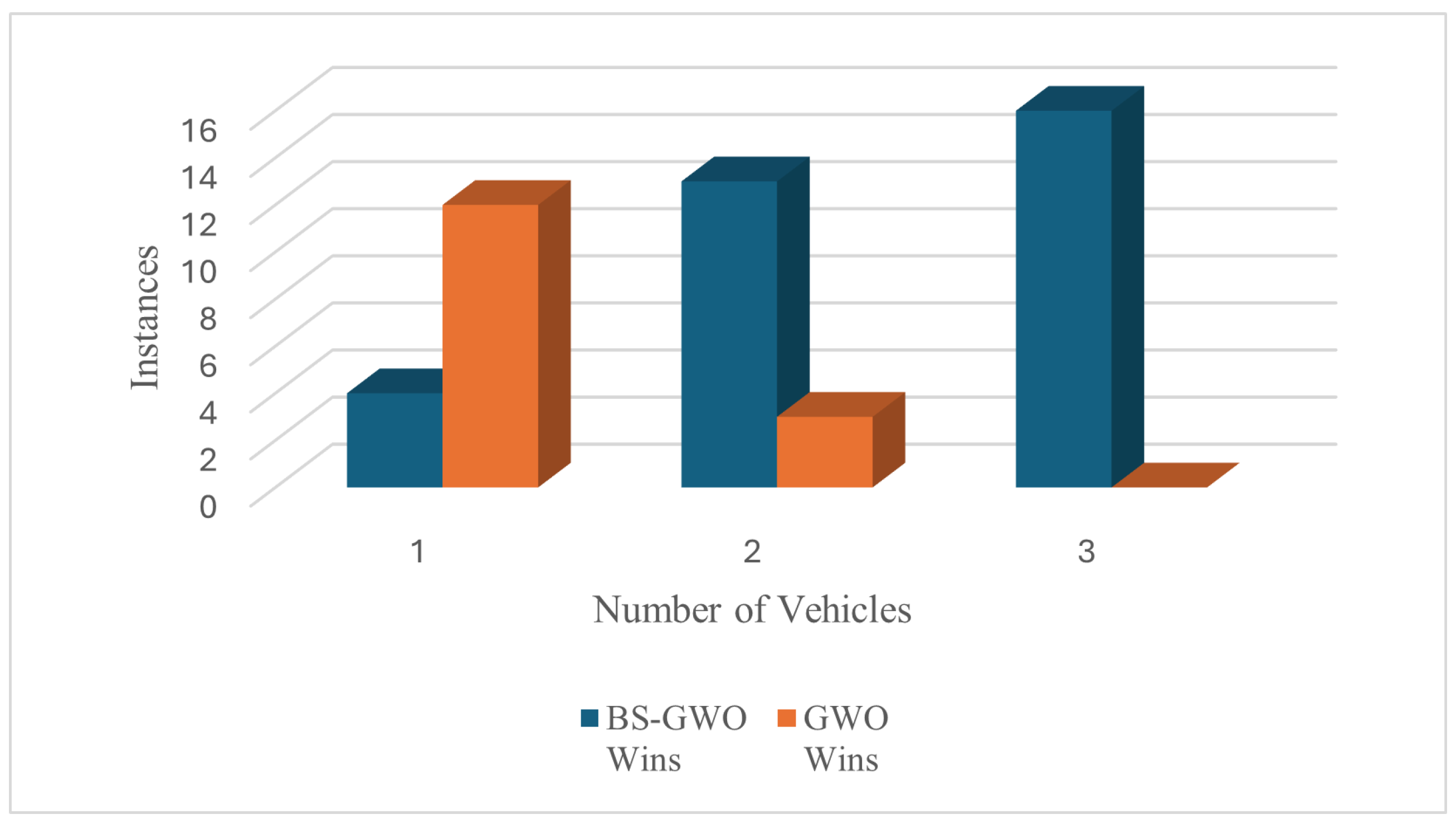
Figure 4.
Comparison between BS-GWO and classical GWO by number of suppliers.
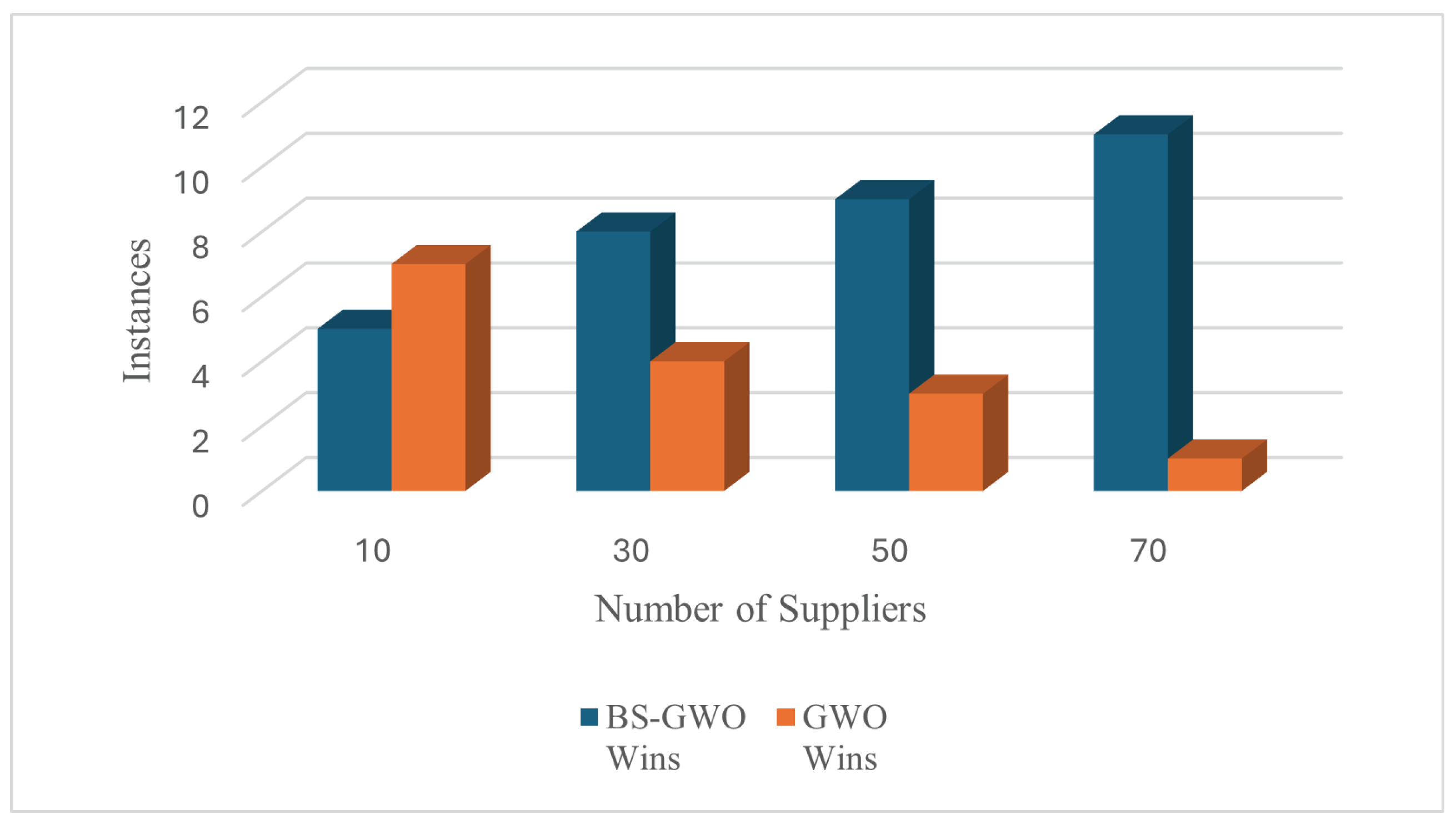

Table 1.
Indices, parameters, and decision variables of the order allocation model.
| Category | Symbol | Description |
|---|---|---|
| Indices | ||
| i | Supplier index, . | |
| o | Product index, . | |
| Parameters | ||
| Demand of product o (units/year). | ||
| Annual production available from supplier i for product o (units/year). | ||
| Setup cost for supplier i and product o ($/setup). | ||
| Unit weight of product o (kg/unit). | ||
| C | Vehicle capacity (kg/vehicle). | |
| R | Number of available vehicles (units). | |
| Decision Variables | ||
| Proportion of the total demand of product o assigned to supplier i. | ||
| T | Production/collection cycle time. |
Table 2.
Indices, parameters, and decision variables of the SDVRP model.
| Category | Symbol | Description |
|---|---|---|
| Sets and Indices | ||
| S | Set of all nodes, including depot node 0 and supplier nodes . | |
| N | Set of suppliers, , indexed by . | |
| Node indices used to define arcs between nodes in S. | ||
| o | Product index, . | |
| v | Vehicle index, . | |
| Parameters | ||
| Fixed cost associated with the use of vehicle v ($/vehicle). | ||
| Variable cost per distance unit traveled by vehicle v ($/km). | ||
| Distance between nodes i and j (km). | ||
| Travel time between nodes i and j (h). | ||
| Loading time at supplier i (h). | ||
| Unloading time associated with supplier i (h). | ||
| Maximum capacity of vehicle v (kg). | ||
| Unit weight of product o (kg/unit). | ||
| M | Large constant used in Big-M constraints. | |
| Demand of product o (units/year). | ||
| Annual production of supplier i for product o (units/year). | ||
| Proportion of the total demand of product o assigned to supplier i. | ||
| T | Production/collection cycle time. | |
| Quantity of product o to be collected from supplier i, given by Equation (1). | ||
| R | Number of available vehicles. | |
| Decision Variables | ||
| Binary variable equal to 1 if vehicle v travels from node i to node j, and 0 otherwise. | ||
| Binary variable equal to 1 if vehicle v is used, and 0 otherwise. | ||
| Quantity of product o collected by vehicle v from supplier i. | ||
| Cumulative load of product o in vehicle v after leaving node i. | ||
| Auxiliary variable for subtour elimination. |
Table 3.
Factors and levels for BS-GWO.
| Parameter | Low Level | High Level |
|---|---|---|
| Number of individuals | 100 | 500 |
| Number of iterations | 200 | 1000 |
| 1 | ||
Table 4.
Ten best BS-GWO configurations according to average rank.
| No. | Ind. | Iter. | Average Objective Function | FO Ranking by Supplier Group | Avg. Rank | ||||||||||
|---|---|---|---|---|---|---|---|---|---|---|---|---|---|---|---|
| 10 | 30 | 50 | 70 | 10 | 30 | 50 | 70 | ||||||||
| 49 | 500 | 1000 | 0.3 | 0.2 | 0.1 | 0.1 | 37.782 | 454.231 | 1876.294 | 4355.681 | 5 | 3 | 6 | 2 | 4.00 |
| 57 | 500 | 1000 | 1.5 | 0.2 | 0.1 | 0.1 | 35.168 | 443.468 | 1834.020 | 4851.051 | 1 | 2 | 3 | 12 | 4.50 |
| 51 | 500 | 1000 | 0.3 | 0.2 | 0.5 | 0.1 | 39.506 | 490.315 | 1842.561 | 4418.882 | 9 | 8 | 4 | 4 | 6.25 |
| 59 | 500 | 1000 | 1.5 | 0.2 | 0.5 | 0.1 | 35.793 | 492.582 | 1988.940 | 4915.735 | 2 | 9 | 10 | 18 | 9.75 |
| 18 | 100 | 1000 | 0.3 | 0.2 | 0.1 | 0.5 | 41.383 | 508.505 | 1977.709 | 4731.876 | 13 | 12 | 9 | 7 | 10.25 |
| 17 | 100 | 1000 | 0.3 | 0.2 | 0.1 | 0.1 | 42.346 | 529.923 | 1941.593 | 4830.044 | 15 | 17 | 7 | 10 | 12.25 |
| 25 | 100 | 1000 | 1.5 | 0.2 | 0.1 | 0.1 | 37.132 | 485.783 | 2029.212 | 5163.691 | 4 | 5 | 16 | 24 | 12.25 |
| 20 | 100 | 1000 | 0.3 | 0.2 | 0.5 | 0.5 | 43.051 | 540.831 | 1965.536 | 4672.899 | 18 | 20 | 8 | 5 | 12.75 |
| 61 | 500 | 1000 | 1.5 | 1.0 | 0.1 | 0.1 | 39.398 | 524.370 | 1999.557 | 5062.341 | 8 | 15 | 12 | 22 | 14.25 |
| 26 | 100 | 1000 | 1.5 | 0.2 | 0.1 | 0.5 | 39.795 | 488.250 | 2028.103 | 5394.846 | 10 | 7 | 15 | 30 | 15.50 |
Table 5.
Global summary of the comparison between BS-GWO and classical GWO.
| Indicator | BS-GWO | Classical GWO |
|---|---|---|
| Number of best objective function | 33 | 15 |
| Significant differences in favor | 30 | 5 |
| Non-significant cases | 3 | 10 |
| Percentage of wins across the 48 instances | 68.75% | 31.25% |
| Number of best execution time | 19 | 29 |
| Significant differences in favor | 8 | 8 |
| Non-significant cases | 11 | 21 |
| Percentage of wins across the 48 instances | 39.58% | 60.42% |
Table 6.
Average objective-function values obtained by each metaheuristic across the 48 instances.
| No. | Instances | Metaheuristics | ||||||
|---|---|---|---|---|---|---|---|---|
| n | O | V | ACO | BS-GWO | MPA | PSO | WOA | |
| 1 | 10 | 5 | 1 | 1.202 | 1.237 | 1.202 | 1.225 | 1.202 |
| 2 | 10 | 5 | 2 | 1.657 | 1.578 | 1.489 | 1.611 | 1.984 |
| 3 | 10 | 5 | 3 | 3.382 | 3.102 | 2.943 | 3.198 | 6.028 |
| 4 | 10 | 10 | 1 | 4.829 | 5.327 | 4.825 | 5.154 | 4.921 |
| 5 | 10 | 10 | 2 | 5.961 | 5.479 | 4.516 | 5.749 | 20.519 |
| 6 | 10 | 10 | 3 | 34.052 | 26.814 | 27.391 | 33.035 | 68.846 |
| 7 | 10 | 20 | 1 | 32.212 | 33.472 | 32.212 | 32.949 | 32.441 |
| 8 | 10 | 20 | 2 | 80.686 | 84.485 | 79.536 | 84.288 | 108.723 |
| 9 | 10 | 20 | 3 | 47.074 | 38.283 | 37.747 | 43.392 | 153.704 |
| 10 | 10 | 30 | 1 | 39.664 | 41.972 | 39.664 | 41.055 | 39.664 |
| 11 | 10 | 30 | 2 | 107.212 | 114.431 | 105.859 | 116.621 | 154.470 |
| 12 | 10 | 30 | 3 | 119.110 | 111.692 | 106.333 | 119.679 | 226.052 |
| 13 | 30 | 5 | 1 | 56.155 | 74.038 | 54.403 | 77.790 | 76.664 |
| 14 | 30 | 5 | 2 | 209.345 | 125.109 | 156.739 | 157.018 | 288.248 |
| 15 | 30 | 5 | 3 | 548.637 | 380.295 | 450.842 | 476.549 | 770.840 |
| 16 | 30 | 10 | 1 | 101.851 | 133.787 | 96.203 | 127.656 | 131.549 |
| 17 | 30 | 10 | 2 | 321.125 | 222.363 | 254.384 | 247.666 | 415.082 |
| 18 | 30 | 10 | 3 | 625.127 | 400.977 | 496.050 | 501.672 | 982.216 |
| 19 | 30 | 20 | 1 | 136.599 | 158.723 | 132.603 | 169.720 | 170.326 |
| 20 | 30 | 20 | 2 | 414.787 | 288.422 | 338.496 | 325.400 | 532.452 |
| 21 | 30 | 20 | 3 | 707.637 | 484.609 | 566.983 | 572.642 | 1273.282 |
| 22 | 30 | 30 | 1 | 231.005 | 278.992 | 210.994 | 271.535 | 276.214 |
| 23 | 30 | 30 | 2 | 467.997 | 353.599 | 395.370 | 390.143 | 670.879 |
| 24 | 30 | 30 | 3 | 909.967 | 654.822 | 753.209 | 717.827 | 1677.813 |
| 25 | 50 | 5 | 1 | 388.946 | 364.559 | 329.977 | 375.195 | 433.085 |
| 26 | 50 | 5 | 2 | 1379.511 | 870.095 | 1063.754 | 960.187 | 1593.167 |
| 27 | 50 | 5 | 3 | 1980.983 | 1315.964 | 1673.654 | 1624.084 | 2646.019 |
| 28 | 50 | 10 | 1 | 463.699 | 509.772 | 442.370 | 519.030 | 623.953 |
| 29 | 50 | 10 | 2 | 1715.055 | 1078.626 | 1293.915 | 1211.564 | 2100.704 |
| 30 | 50 | 10 | 3 | 2089.893 | 1362.380 | 1721.221 | 1725.328 | 3035.708 |
| 31 | 50 | 20 | 1 | 643.868 | 643.274 | 615.890 | 664.167 | 781.183 |
| 32 | 50 | 20 | 2 | 1410.913 | 899.607 | 1110.070 | 1034.637 | 1679.835 |
| 33 | 50 | 20 | 3 | 2787.683 | 1863.146 | 2275.985 | 2141.180 | 4046.098 |
| 34 | 50 | 30 | 1 | 1626.073 | 1806.397 | 1696.313 | 1905.333 | 2221.485 |
| 35 | 50 | 30 | 2 | 3846.973 | 2600.693 | 3051.748 | 2820.101 | 5028.762 |
| 36 | 50 | 30 | 3 | 3227.834 | 2071.777 | 2650.318 | 2409.563 | 4384.942 |
| 37 | 70 | 5 | 1 | 5052.223 | 3815.187 | 3664.982 | 3511.073 | 4503.789 |
| 38 | 70 | 5 | 2 | 5420.777 | 3652.971 | 4265.039 | 3739.980 | 6018.023 |
| 39 | 70 | 5 | 3 | 8737.847 | 5535.028 | 7302.286 | 6067.693 | 9733.983 |
| 40 | 70 | 10 | 1 | 2052.372 | 1482.056 | 1513.776 | 1512.071 | 1903.011 |
| 41 | 70 | 10 | 2 | 1346.330 | 897.905 | 1055.982 | 933.113 | 1179.183 |
| 42 | 70 | 10 | 3 | 3977.329 | 2398.461 | 3078.805 | 2779.572 | 4326.775 |
| 43 | 70 | 20 | 1 | 4731.495 | 3314.122 | 4050.131 | 3957.697 | 5717.289 |
| 44 | 70 | 20 | 2 | 3545.699 | 2151.138 | 2738.621 | 2542.963 | 3934.458 |
| 45 | 70 | 20 | 3 | 6504.047 | 4006.562 | 5398.476 | 4704.760 | 7047.468 |
| 46 | 70 | 30 | 1 | 3124.176 | 2004.131 | 2334.577 | 2066.004 | 2679.315 |
| 47 | 70 | 30 | 2 | 4571.222 | 2798.856 | 3597.637 | 3153.594 | 5084.350 |
| 48 | 70 | 30 | 3 | 6610.140 | 4597.873 | 5443.812 | 4896.920 | 7864.078 |
Table 7.
Average RPD performance of the metaheuristics.
| Algorithm | ACO | BS-GWO | MPA | PSO | WOA |
|---|---|---|---|---|---|
| Average RPD | 22.7431 | 4.3707 | 9.9327 | 12.0355 | 39.0438 |
| Ranking | 4 | 1 | 2 | 3 | 5 |
Table 8.
Pairwise comparative results between BS-GWO and the competing metaheuristics.
| Algorithm | Best-Value | BS-GWO Better | BS-GWO Worse | BS-GWO Equal |
|---|---|---|---|---|
| BS-GWO | 28 | – | – | – |
| MPA | 18 | 26 | 17 | 5 |
| ACO | 4 | 33 | 12 | 3 |
| PSO | 1 | 28 | 2 | 18 |
| WOA | 2 | 41 | 4 | 3 |
Disclaimer/Publisher’s Note: The statements, opinions and data contained in all publications are solely those of the individual author(s) and contributor(s) and not of MDPI and/or the editor(s). MDPI and/or the editor(s) disclaim responsibility for any injury to people or property resulting from any ideas, methods, instructions or products referred to in the content. |
© 2026 by the authors. Licensee MDPI, Basel, Switzerland. This article is an open access article distributed under the terms and conditions of the Creative Commons Attribution (CC BY) license (http://creativecommons.org/licenses/by/4.0/).
Copyright: This open access article is published under a Creative Commons CC BY 4.0 license, which permit the free download, distribution, and reuse, provided that the author and preprint are cited in any reuse.


