

Submitted:
06 July 2026
Posted:
07 July 2026
You are already at the latest version
Abstract
Highway–rail grade crossing (HRGC) safety has improved substantially over recent decades through engineering upgrades, active warning systems, crossing closures, enforcement, and public education. Recent national trends, however, suggest that these gains may have slowed, raising the question of whether HRGC safety has entered a persistent plateau. This study investigates whether the historical decline in U.S. HRGC incidents has transitioned into a statistically distinct safety regime and whether the factors associated with casualty occurrence have changed following that transition. An analytical framework integrating regime-transition analysis, cross-regime casualty comparison, and explainable machine learning was applied to nationwide Federal Railroad Administration incident records from 1976 to 2025. Trend analysis, complementary stationarity diagnostics, residual diagnostics, information criteria, and sensitivity analysis consistently identified 2012 as the onset of a statistically stationary safety plateau. Comparison of casualty outcomes showed no meaningful change in either the probability of casualty occurrence or the distribution of injury and fatality outcomes following the transition. Explainable random forest models further demonstrated substantial temporal stability in the factors associated with casualty occurrence. Train speed, vehicle occupancy, driver presence, and highway-user actions remained the dominant predictors across both safety regimes, with driver presence ranking among the most influential characteristics during the plateau period. These findings indicate that the current safety challenge is not the emergence of new collision mechanisms but the persistence of well-established operational and behavioral risk factors. Future reductions in HRGC casualties will likely require targeted engineering improvements, advanced warning technologies, connected-vehicle and vehicle-to-infrastructure systems, artificial intelligence–enabled monitoring, and focused public education to address the persistent residual risks sustaining the national safety plateau.
Keywords:
transportation safety
; safety persistence
; stationarity analysis
; structural break analysis
; casualty prediction
; decision support
; intelligent transportation systems
1. Introduction
Highway–rail grade crossings (HRGCs) remain one of the most challenging locations within multimodal transportation systems because they require roadway users and trains to safely share the same physical space. Although collisions occur relatively infrequently compared with other roadway crashes, they often result in severe consequences due to the large mass and momentum of trains [1]. Consequently, reducing HRGC incidents has remained a long-standing priority for transportation agencies through engineering improvements, active warning systems, crossing closures, public education, enforcement, and regulatory initiatives.
These efforts have contributed to substantial reductions in HRGC incidents over the past several decades. National statistics indicate that annual collisions declined steadily throughout the late 20th century and early 21st century as crossing infrastructure improved and safety programs became more widely implemented [2]. Visual inspection of recent national trends, however, suggests that this historical decline has slowed considerably, raising the possibility that HRGC safety has entered a period in which further reductions are increasingly difficult to achieve. If such a plateau exists, it would imply that conventional safety strategies have approached diminishing returns and that future progress may require fundamentally different approaches.
Despite the practical importance of this question, relatively little research has examined whether the apparent stabilization in national HRGC incidents represents a statistically distinct safety regime or merely short-term variation within a continuing downward trend. Most previous studies have focused on identifying factors associated with collision occurrence or casualty severity using statistical or machine-learning (ML) models [3], whereas comparatively little attention has been given to determining whether the underlying safety process itself has changed over time. Establishing the existence of a persistent safety plateau is important because it provides the context for interpreting contemporary HRGC risks and for determining whether existing countermeasures continue to address the dominant collision mechanisms.
An equally important question concerns whether the characteristics associated with casualty occurrence have evolved following the apparent transition to the plateau. If the dominant determinants of casualty outcomes have changed, then future engineering investments and policy interventions should be redirected toward newly emerging risk factors. Conversely, if the same operational and behavioral mechanisms continue to dominate casualty occurrence, the challenge becomes identifying why these persistent mechanisms remain resistant to traditional safety improvements. Distinguishing between these alternatives has important implications for prioritizing future investments in engineering design, warning technologies, traffic operations, enforcement, and public education. Recent studies continue to identify driver behavior, train operations, and crossing characteristics as dominant contributors to HRGC safety outcomes [4].
Recent advances in explainable artificial intelligence (AI) provide new opportunities to address this problem. ML models have demonstrated strong predictive capability for transportation safety applications, yet many operate as black boxes that provide limited insight into the factors driving their predictions. Explainable methods based on Shapley additive explanations (SHAP) overcome this limitation by quantifying both the relative importance and directional influence of individual predictors [5]. When applied separately to different historical safety regimes, explainable ML enables direct comparison of the incident characteristics associated with casualty occurrence over time.
The goal of this study is to determine whether the long-term decline in U.S. HRGC incidents has transitioned into a statistically persistent safety plateau and to evaluate whether the incident characteristics associated with casualty occurrence have changed following that transition. To achieve this goal, the study develops an analytical framework that integrates statistical regime-transition analysis, cross-regime casualty comparison, and explainable ML using nationwide Federal Railroad Administration (FRA) incident records spanning 1976 through 2025.
The study makes four principal contributions. First, it introduces a statistically based regime-transition framework that identifies the onset of a persistent HRGC safety plateau using complementary trend, stationarity, residual, information-criterion, and sensitivity analyses rather than conventional breakpoint methods based solely on model fit. Second, it evaluates whether casualty occurrence and casualty severity changed following the transition to the plateau, thereby distinguishing changes in collision frequency from changes in collision consequences. Third, it compares explainable ML models across the declining and plateau safety regimes to identify both persistent and emerging incident characteristics associated with casualty occurrence. Fourth, it demonstrates how integrating statistical inference with explainable AI can support more targeted engineering, operational, and policy interventions aimed at overcoming the current HRGC safety plateau through data-driven infrastructure improvements, advanced warning technologies, connected-vehicle and vehicle-to-infrastructure systems, AI, and focused public education.
The remainder of this paper is organized as follows. Section 2 reviews previous research on HRGC safety, temporal safety trends, and explainable AI. Section 3 describes the analytical framework, including data preparation, regime-transition analysis, casualty comparison, random forest (RF) modeling, and SHAP-based interpretation. Section 4 presents the empirical results. Section 5 discusses their implications for engineering practice and transportation policy. Section 6 concludes the study with recommendations for future research.
2. Literature Review
Transportation agencies have invested in HRGC safety for several decades through engineering improvements, warning-device modernization, crossing closures, operational controls, enforcement, and public education. These interventions have substantially reduced collision frequency and casualty severity, yet collisions continue to occur because HRGC safety depends on complex interactions among infrastructure, train operations, roadway users, and the surrounding transportation environment. Recent studies continue to demonstrate that improving HRGC safety requires consideration of both engineering and human behavioral factors rather than relying on a single intervention strategy [4].
2.1. Highway–Rail Grade Crossing Safety
Previous HRGC research has consistently identified train operations, roadway geometry, warning devices, traffic exposure, and driver behavior as primary contributors to collision occurrence and casualty severity [6,7]. Statistical and ML models have both demonstrated that these factors interact in complex, nonlinear ways that are difficult to capture using conventional linear approaches [3]. Several recent studies have focused specifically on crash severity rather than collision frequency [8]. Mixed-effects and heterogeneity-based models showed that train speed, vehicle type, lighting conditions, and roadway characteristics remain important determinants of severe HRGC outcomes [9]. Similar findings have been reported using causal inference and graphical modeling approaches, which identified operational and infrastructure characteristics as important contributors to collision risk [6]. Infrastructure quality also remains an active area of investigation. Studies examining crossing inventory databases reported that prediction performance depends strongly on the completeness and accuracy of inventory information, emphasizing the importance of reliable infrastructure data for safety analysis [10]. Subsequent work demonstrated that inventory verification further improves crash prediction accuracy and model reliability [11].
Engineering countermeasures continue to receive considerable attention. Before-and-after evaluations using empirical Bayes methods demonstrated measurable safety improvements following installation of active warning systems [2]. Other recent investigations examined roadway design through microsimulation [12], passive-crossing visibility enhancements [13], safety inspection procedures [14], and roadway-user violations [15], collectively reinforcing the importance of engineering treatments tailored to crossing-specific operating conditions.
Human behavior remains another dominant research theme. Driver knowledge, decision-making, and compliance with warning devices continue to influence HRGC safety outcomes, even at crossings equipped with active protection [16]. Studies of roadway-user behavior similarly identified risky maneuvers, improper crossing decisions, and gate violations as recurring contributors to collision occurrence [4]. Recent investigations have also examined emerging operational conditions. For example, comparisons before and during the COVID-19 pandemic demonstrated that changes in travel patterns can influence the factors associated with HRGC injury severity, illustrating the importance of considering temporal variation when evaluating safety performance [17]. Although these studies substantially advance understanding of HRGC safety, most analyze historical data as a single population, implicitly assuming that the underlying safety process remains stable throughout the study period.
2.2. Temporal Evolution of Transportation Safety
Transportation safety research has long relied on historical trend analysis to evaluate the effectiveness of engineering improvements and policy interventions. Regression models, structural-break analysis, and change-point detection methods have frequently been used to identify shifts in long-term safety performance. Most breakpoint studies, however, identify transition years that maximize improvements in statistical fit or minimize residual error [18]. Such approaches effectively detect changes in trend magnitude but do not necessarily determine when a transportation system enters a statistically persistent operating regime. Consequently, relatively little research has evaluated whether apparent stabilization in national safety performance represents a genuine stationary process rather than a slowing decline. This limitation is particularly important for HRGC safety because identifying the onset of a persistent plateau changes the interpretation of future safety investments. A continuing downward trend suggests that existing interventions remain effective, whereas a statistically persistent plateau indicates that conventional approaches may be approaching diminishing returns.
2.3. Machine Learning and Explainable Artificial Intelligence
ML methods have become increasingly common in transportation safety [19]. ML models accommodate nonlinear relationships, complex interactions, heterogeneous predictor effects, and mixed data types without restrictive distributional assumptions [20]. Comparative evaluations consistently reported that ensemble-learning methods frequently outperform conventional statistical models when predicting crash severity [21]. Recent advances have further expanded the range of predictive models applied to transportation safety, including deep neural networks [5], transfer learning [22], transformers [23], optimized boosting algorithms [24], ensemble methods [25], and convolutional neural networks [26]. These methods generally improve predictive performance while capturing increasingly complex relationships among crash characteristics. Despite these advances, predictive performance alone provides limited value for engineering decision-making unless model predictions can also be interpreted. This limitation has motivated growing interest in explainable AI, particularly SHAP, which quantifies both predictor importance and directional influence.
Recent transportation studies increasingly integrated SHAP with ML models to interpret crash severity across diverse operating environments, including urban intersections [27,28], freeways [7,29,30], work zones [31], motorcycle crashes [32,33], nighttime crashes [34], vulnerable-road-user crashes [35,36], defective-vehicle crashes [37], weather-related crashes [38], farm equipment crashes [39], and cross-cultural safety analyses [40,41]. Collectively, these studies demonstrated that explainable ML improves transparency while preserving predictive capability. They also showed that operational, behavioral, environmental, and infrastructure variables interact in complex ways that vary across transportation systems. Nevertheless, most explainable ML studies analyzed observations from a single historical period. Predictor importance therefore represented an average relationship across the entire dataset, making it difficult to determine whether the mechanisms associated with severe outcomes remained stable or evolved as transportation systems changed over time.
2.4. Research Gaps
The literature reveals three important gaps. First, previous HRGC research has extensively investigated collision occurrence and crash severity [22,42,43], but has provided limited evidence regarding whether the apparent stabilization in national incident frequency represents a statistically persistent safety regime. Existing temporal analyses generally emphasized changes in trend magnitude rather than identifying the earliest period exhibiting the statistical characteristics of persistence. Second, previous studies generally examined complete historical datasets without evaluating whether the characteristics associated with casualty occurrence changed following the apparent transition to the modern safety plateau. Consequently, it remains unclear whether the residual national collision burden reflects emerging risk factors or the continued persistence of long-established operational and behavioral mechanisms. Third, although explainable ML has substantially improved interpretation of transportation safety models, it has rarely been integrated with statistical regime-transition analysis to evaluate how predictor importance changes across distinct historical safety regimes. Combining complementary time-series diagnostics with explainable ML provides an opportunity to relate changes in long-term safety performance directly to changes in the factors associated with casualty occurrence.
This study addresses these gaps by developing an integrated analytical framework that combines statistical regime-transition analysis, cross-regime casualty comparison, and explainable ML. The framework first identifies the onset of a statistically persistent HRGC safety plateau using complementary trend, stationarity, residual, information-criterion, and sensitivity analyses. It then evaluates whether casualty occurrence and severity changed following the transition and finally compares explainable RF models developed separately for the declining and plateau regimes. Together, these analyses determine whether the dominant mechanisms associated with casualty occurrence have evolved or remained stable and provide evidence to support more targeted engineering, operational, technological, and educational strategies for reducing the persistent residual risks that continue to sustain the modern HRGC safety plateau.
3. Methodology
Figure 1 illustrates the analytical workflow that sought to identify the incident-level characteristics most strongly associated with casualty outcomes and to determine whether the relative importance of these characteristics changed between the declining safety regime (Epoch 0) and the subsequent plateau regime (Epoch 1), with epoch boundaries determined by a breakpoint analysis. The workflow implemented all functions in Python version 3.12 with packages for regime-change diagnostics (statsmodels version 0.14.6), classification and feature importance (scikit-learn version 1.8.1), and model explainability (SHAP version 0.52.0).
3.1. Data Preparation
Large administrative transportation databases contain sparse variables, redundant descriptors, inconsistent coding, and heterogeneous operating conditions that can reduce the effectiveness of statistical and ML analyses. Therefore, the FRA Form 57 incident records were processed using a structured six-stage data preparation workflow designed to produce a consistent analytical dataset while preserving the dominant operating characteristics of HRGC incidents.
The workflow first removed variables with more than 80% missing values. The dataset was then restricted to public HRGCs within the contiguous United States (CONUS), and county assignments were reconciled using the previously developed hierarchical multistage inference (HMI) procedure to correct geographic coding inconsistencies [44]. Redundant text descriptors, administrative metadata, and variables containing excessive unknown or missing values were subsequently removed. To reduce structural heterogeneity, the analysis retained incidents involving Class I freight railroads operating freight trains on mainline track under common warning-device configurations and excluded incidents involving hazardous material releases or reported sight obstructions. Low-frequency categorical levels were consolidated by retaining the dominant operating categories, while numerical variables were constrained to domain-informed ranges to remove implausible values. Records from incomplete boundary years were also excluded to ensure consistent annual comparisons.
Finally, injury and fatality counts were combined into a binary casualty outcome, warning-device categories were grouped into four major classes, and records with remaining missing values in retained analytical variables were removed. The resulting dataset provided a lower-dimensional, internally consistent representation of HRGC incidents suitable for the subsequent statistical and explainable ML analyses.
3.2. Trend Breakpoint Identification
The objective of this stage was to identify the onset of the HRGC incident plateau and establish a statistically informed separation between the historical period of sustained incident reduction (Epoch 0) and the subsequent period of persistence (Epoch 1). Conventional structural-break procedures typically identify the year that maximizes improvement in model fit. Such methods are useful for detecting changes in trend magnitude but do not necessarily identify the onset of a stable regime. The present study instead defined the breakpoint as the earliest year after which annual incident counts became statistically consistent with a stationary process. This definition aligns directly with the substantive objective of determining when the long-term decline in HRGC incidents effectively ceased and a persistent safety plateau (Epoch 1) emerged.
Candidate Breakpoint Evaluation: An exhaustive search was performed across all feasible candidate transition years, denoted by τ. For each candidate year, the annual series was partitioned into two segments: and . The pre-transition segment represented a candidate Epoch 0 regime, whereas the post-transition segment represented a candidate Epoch 1 regime.
Trend Assessment: The first requirement for a plateau regime is the absence of a statistically meaningful trend. To evaluate this condition, separate linear regression models were fitted to the Epoch 0 and Epoch 1 segments. For the Epoch 0 period:
For the Epoch 1 period:
where:
- = total incidents in year
- = slope of the Epoch 0 regime
- = slope of the candidate Epoch 1 regime
- = random error term
The Epoch 0 period was expected to exhibit a significant negative slope where with . The candidate Epoch 1 period was required to exhibit no statistically significant trend such that and . These conditions ensure that any remaining changes in annual incident counts are statistically indistinguishable from zero.
Stationarity Assessment: A non-significant slope alone does not guarantee that a time series has reached a stable regime. A series may exhibit little apparent trend while still containing non-stationary behavior. Therefore, stationarity was evaluated using both the Kwiatkowski-Phillips-Schmidt-Shin (KPSS) and Augmented Dickey–Fuller (ADF) diagnostics [45]. The KPSS diagnostic evaluates whether a series is stationary around a constant mean. Its hypotheses are H0 (series is stationary) and HA (series is non-stationary). A candidate plateau period was considered consistent with stationarity when . The KPSS diagnostic was selected because its null hypothesis directly corresponds to the desired plateau condition. The ADF diagnostic evaluates the complementary question of whether a series contains a unit root. Its hypotheses are H0 (series contains a unit root) and HA (series in stationary). Evidence against a unit root was established when .
The combined use of KPSS and ADF provides stronger evidence than either diagnostic alone. The KPSS diagnostic evaluates whether stationarity can be accepted, whereas the ADF diagnostic evaluates whether non-stationarity can be rejected. Agreement between the two diagnostics provides greater confidence that the observed plateau in Epoch 1 represents a genuinely stable regime rather than an artifact of limited sample length.
The complementary diagnostics used in this study were not treated as repeated hypothesis tests of a common null hypothesis. Instead, each procedure evaluated a different statistical property of the candidate post-transition series, including trend, stationarity, unit-root behavior, and residual independence. A candidate breakpoint was accepted only when all predefined diagnostic criteria were simultaneously satisfied. Consequently, the diagnostics served as corroborating evidence rather than multiple opportunities to reject the same hypothesis.
Residual Independence Assessment: Even when a series is trendless and stationary, residual temporal dependence may still be present. Therefore, the Ljung–Box diagnostic was applied to evaluate whether fluctuations around the plateau mean behaved as random noise. The plateau model was represented as:
where is the mean annual incident count during the candidate plateau period. The Ljung–Box statistic is:
where:
- n = number of observations
- h = number of lags evaluated
- = autocorrelation coefficient at lag k
The corresponding hypotheses are and . A candidate plateau period was considered free of meaningful temporal dependence when . The Ljung–Box diagnostic complements the KPSS and ADF diagnostics by evaluating a different property of the series. Whereas KPSS and ADF assess stationarity, the Ljung–Box diagnostic evaluates whether the remaining fluctuations occur randomly or retain systematic temporal structure. Together, the three diagnostics provide a comprehensive assessment of persistence.
Breakpoint Selection: The candidate years were not evaluated as competing statistical hypotheses from which the most significant result was selected. Rather, the search served as a deterministic algorithm for identifying the earliest year satisfying a prespecified definition of a persistent safety regime. Consequently, candidate years failing any diagnostic criterion were rejected regardless of their relative statistical significance. A candidate year was classified as the onset of a plateau regime only if all diagnostic conditions were satisfied simultaneously. Hence, the selected breakpoint was defined as the earliest year satisfying these conditions:
where is the estimated onset of a persistent plateau regime. This criterion identifies the first year at which the long-term decline ceased, and annual incident counts became statistically consistent with a stable process. As established above, simultaneous agreement across all diagnostics reflects corroborating evidence for a persistent regime rather than repeated testing of a common null hypothesis.
Buffer-Year Sensitivity Analysis: A sensitivity analysis was conducted to determine whether transition years near the breakpoint should be removed to improve separation between the declining and plateau regimes. Symmetric buffers were evaluated around the selected breakpoint:
where b is the buffer width in years. Candidate buffers were assessed using the same trend, stationarity, and residual-independence diagnostics described above. The final buffer was selected as the smallest exclusion window that maintained a statistically significant pre-transition decline and a statistically stationary post-transition plateau. This approach minimized the removal of valid observations while avoiding contamination between the two regimes.
Information-Criterion Validation: The breakpoint identified from the trend and stationarity diagnostics was independently evaluated using information criteria to determine whether it also provided the most parsimonious representation of the annual incident series. For each candidate breakpoint, the Epoch 0 was modeled using linear regression, whereas the Epoch 1 was modeled as a constant-mean (plateau) process. The residual sum of squares (RSS) errors from the two regimes were first combined to quantify the overall model error:
The combined residual error was then used to compute the Akaike information criterion (AIC) and Bayesian information criterion (BIC) as
and
where:
- n is the number of annual observations
- k is the total number of estimated model parameters
Both information criteria balance model fit against model complexity, with smaller values indicating a more parsimonious representation of the data.
The candidate plateau period necessarily contains fewer annual observations than the historical declining regime because the objective is to identify the earliest onset of persistence. Consequently, no individual stationarity diagnostic was interpreted in isolation. Instead, the KPSS, ADF, and Ljung–Box diagnostics were considered jointly with the post-transition trend estimate, confidence interval, information-criterion analysis, and transition-buffer sensitivity analysis to evaluate whether the annual incident series exhibited behavior consistent with a persistent safety regime. Since the information criteria and transition-buffer sensitivity analysis served as independent corroborating assessments rather than additional selection criteria, their agreement with the diagnostic-based breakpoint strengthens confidence that the identified transition reflects a genuine change in the long-term behavior of the annual incident series.
3.3. Cross Regime Casualty Analysis
To determine whether the transition from Epoch 0 to Epoch 1 was accompanied by changes in incident outcomes, casualty occurrence and outcome composition were compared between the two periods. This analysis complemented the regime-transition analysis by evaluating whether the stabilization in annual incident counts was accompanied by changes in the probability or severity of casualty outcomes. Incident outcomes were derived directly from the FRA Form 57 injury and fatality counts. The total number of casualties associated with each incident was calculated as
where:
- Ci is the total casualties for incident i
- Ki is the number of fatalities reported for incident i
- Ii is the number of injuries reported for incident i
Each incident was then classified according to casualty occurrence as
where the ML target variable was:
- Y = 1 denotes an incident involving at least one injury or fatality (casualty)
- Y = 0 denotes an incident involving no reported injuries or fatalities (non-casualty)
To evaluate whether the probability of a casualty differed between the two safety regimes, the casualty proportions were calculated as
where:
- is the observed casualty proportion
- x is the number of casualty incidents
- n is the total number of incidents within the corresponding regime
The equality of casualty proportions between the two epochs was evaluated using a two-proportion z-test. Under the null hypothesis that both regimes share the same casualty probability, the test statistic is
where:
- and are the observed casualty proportions for the two regimes
- n1 and n2 are the corresponding sample sizes
- is the pooled casualty proportion
Although the casualty proportion indicates whether the likelihood of injury or fatality changed over time, it does not distinguish between injury and fatality outcomes. Therefore, a second analysis examined the composition of incident outcomes using three mutually exclusive categories:
- Non-casualty Ci = 0
- Injury Ii > 0 and Ki = 0
- Fatality Ki > 0
The association between safety regime and outcome composition was evaluated using Pearson’s chi-square diagnostic of independence. The test statistic is
where:
- is the observed frequency in cell (i, j)
- is the corresponding expected frequency assuming independence
- r is the number of rows
- c is the number of outcome categories
Since large sample sizes can produce statistically significant chi-square results for very small distributional differences, practical significance was evaluated using Cramer’s V:
where:
- is the chi-square statistic
- n is the total number of observations
- k is the smaller of the number of rows or columns in the contingency table
The two statistical diagnostics provide complementary information. The two-proportion z-test evaluates whether the overall probability that an incident results in one or more casualties changed between the two safety regimes. In contrast, the chi-square diagnostic determines whether the distribution of incident outcomes among non-casualty, injury, and fatality categories changed, irrespective of the overall casualty rate. Finally, Cramer’s V quantifies the practical magnitude of any statistically significant differences detected by the chi-square diagnostic. Collectively, these analyses distinguish whether the safety plateau of Epoch 1 reflects changes in the frequency of casualty-producing incidents, changes in the composition of injury and fatality outcomes, or both. Since the two-proportion z-test and chi-square diagnostic address different inferential questions rather than repeated tests of a common hypothesis, no multiplicity adjustment was applied.
3.4. One-Hot Encoding
All categorical predictors were transformed using one-hot encoding (OHE). This approach preserves the nominal nature of categorical variables and avoids imposing artificial ordinal relationships among categories. For a categorical predictor containing K retained levels, a set of binary indicator variables was generated:
where = binary indicator for category and i = incident index. Continuous variables were retained in their original numerical form.
3.5. Random Forest Classification
Separate RF classifiers were developed for Epoch 0 and Epoch 1 to distinguish casualty from non-casualty incidents within each period. RF was selected based on its superior performance in previous HRGC safety research [46]. RF can model nonlinear relationships, higher-order interactions, heterogeneous predictor effects, and mixed data types without requiring distributional assumptions. Since the objective was to identify influential incident characteristics rather than estimate regression coefficients, no pre-model collinearity screening was performed. RF is generally robust to correlated predictors, although correlated variables may share predictive information and consequently distribute feature importance among themselves. The subsequent SHAP analysis was therefore interpreted primarily in terms of the relative importance hierarchy rather than small differences between similarly ranked predictors
Each RF model consists of an ensemble of decision trees generated from bootstrap samples of the training data. The final classification is determined through majority voting among all trees:
where:
- = predicted casualty class
- = prediction from tree b
- B = total number of trees
- = predictor vector
The predictive unit of analysis was the individual HRGC incident rather than the crossing. Consequently, repeated incidents occurring at the same crossing during an epoch were retained because the objective was to identify incident characteristics associated with casualty occurrence rather than to estimate crossing-specific risk or predict future performance at previously unseen crossings. Stratified cross-validation therefore evaluated predictive performance for the incident-level classification task addressed in this study.
The primary evaluation metric was the area under the receiver operating characteristic curve (AUC):
where TPR = true positive rate and u = false positive rate. Precision–recall area under the curve (PR-AUC) and classification accuracy were also computed to assess performance under class imbalance.
3.6. SHAP-Based Model Explanation
Model interpretation was performed using SHAP [47], which quantifies the contribution of each predictor to a model prediction by distributing prediction gains among predictors according to principles from cooperative game theory. For an individual observation, the RF prediction can be expressed as:
where:
- = model prediction
- = baseline prediction
- = SHAP contribution of predictor j
- p = total number of predictors
The SHAP value for predictor j is defined as:
where:
- F = full predictor set
- S = subset of predictors excluding predictor j
- = model prediction using predictor subset S
This formulation estimates the average marginal contribution of predictor j across all possible predictor combinations.
3.6.1. Global Importance Estimation
Global predictor importance was calculated using the mean absolute SHAP value across all observations:
where:
- Ij = global importance of predictor j
- N = number of observations
- = SHAP value of predictor j for observation i
Predictors with larger Ij values exerted greater influence on casualty classification and therefore ranked higher in the importance hierarchy. Closely related predictors may share attribution, so interpretation focused on the dominant hierarchy of influential variables rather than exact differences among adjacent rankings.
The SHAP values were interpreted independently within each epoch-specific RF model. Comparisons between epochs therefore focused on changes in the relative ordering of predictor importance rather than direct comparison of absolute SHAP magnitudes, which may vary with model structure, sample composition, and baseline prediction.
3.6.2. Directional Association Analysis
Although SHAP importance ranking quantifies influence magnitude, it does not indicate whether a predictor increases or decreases the likelihood of casualty occurrence. Therefore, a directional metric was computed using the mean signed SHAP value:
where = average directional contribution of predictor j. Predictors with positive values, Dj > 0, were interpreted as contributing toward casualty occurrence (Y = 1), whereas predictors with negative values, Dj < 0, were interpreted as contributing away from casualty occurrence. This procedure enabled simultaneous evaluation of predictor importance and directional influence.
3.6.3. Epoch Comparison
The workflow finally compared SHAP rankings and directional effects between Epoch 0 and Epoch 1. Changes in predictor rankings were interpreted as shifts in the relative importance of casualty-associated characteristics within each independently trained model, whereas stable rankings indicated persistence of the underlying injury process through time. The comparison emphasized relative rank rather than absolute differences in SHAP magnitude.
The comparison focused on three complementary dimensions:
where:
- = SHAP importance
- = predictor rank
- = directional SHAP effect
This framework allowed identification of both persistent and emerging determinants of casualty outcomes, providing insight into how the relative contributions of train operations, highway-user behavior, vehicle occupancy, warning systems, and environmental conditions evolved between the pre-2010 declining safety era and the post-2010 safety plateau.
4. Results
The following subsections present the results of the data reduction, the regime-transition analysis, the comparison of casualty outcomes between the two safety regimes, and the explainable ML analysis of incident characteristics associated with casualty occurrence.
4.1. Data Reduction
The sequential data preparation procedure progressively reduced dimensionality and analytical noise while preserving the dominant operational characteristics of the FRA incident database (Table 1). The original dataset contained 250,660 incidents described by 154 variables. Sparsity filtering, geographic restriction to public CONUS crossings, and removal of redundant descriptor fields and administrative metadata substantially reduced the number of variables while maintaining the large majority of observations. Geographic reconciliation using the HMI procedure also corrected county assignments before subsequent analyses.
The remaining processing stages restricted the analysis to a more homogeneous operating environment by retaining incidents involving Class I freight railroads operating freight trains on mainline track under common warning-device and operating conditions (Table 2). Additional reductions were achieved by removing infrequent categorical levels, filtering implausible numerical values, and excluding records containing remaining missing values in retained analytical variables (Table 3). Two correlated features were dropped: “Highway User Position Code” due to its correlation with “Highway User Action Code” and “Driver Condition Code” due to its correlation with the definition of casualty. The variables “Year” and “Epoch” were also dropped due to their redundancy after splitting the data into the two epochs. The final analytical dataset contained 61,858 incidents represented by 21 analytical predictors used in the subsequent statistical analyses and RF models. Overall, the preparation workflow emphasized data consistency and reduced noise while retaining the dominant characteristics of the national HRGC incident population.
4.2. Regime Transition and Plateau Identification
Annual HRGC incident counts from 1976 through 2025 were evaluated using an exhaustive breakpoint search combined with trend, stationarity, residual, information-criterion, and sensitivity analyses. Figure 2 shows that 2012 was identified as the earliest year satisfying all plateau-selection criteria. The resulting segmentation defined 1976–2011 (Epoch 0) as the declining regime and 2012–2025 (Epoch 1) as the plateau regime. During Epoch 0, annual incidents declined by approximately 101 incidents per year (95% CI: −109.4 to −92.7, p < 0.001), confirming a sustained long-term reduction in HRGC incidents. In contrast, the Epoch 1 trend was not statistically different from zero (slope = −1.67 incidents/year, 95% CI: −4.59 to 1.25, p = 0.235), indicating that annual incident counts had stabilized.
Table 4 summarizes the complementary statistical diagnostics supporting the selected breakpoint. The KPSS diagnostic failed to reject stationarity (p = 0.10), whereas the ADF diagnostic rejected the presence of a unit root (p = 1.60 × 10⁻⁴). The Ljung–Box diagnostic was also non-significant (p = 0.985), indicating no evidence of residual temporal autocorrelation within the plateau period.
The transition year was further evaluated through complementary robustness assessments, including buffer-year sensitivity analysis and information-criterion comparisons. Buffer widths ranging from zero to four years were examined to determine whether observations surrounding the breakpoint should be excluded to improve separation between the two regimes. The smallest acceptable buffer was zero years, indicating that no transition observations required removal and that the annual series naturally separated into statistically distinct declining and plateau periods.
Independent support for the selected breakpoint was provided by the information-criterion analysis. Both the AIC (AIC = 487.056) and BIC (BIC = 490.862) reached their minimum values for the 2012 transition year, indicating that this breakpoint provided the most parsimonious representation of the annual incident series. Collectively, these complementary diagnostics provided mutually consistent evidence that 2012 was the earliest year satisfying the predefined characteristics of a persistent HRGC safety plateau. The corresponding Epoch 1 period is characterized by statistically stable annual incident counts averaging approximately 187 incidents per year.
4.3. Cross-Regime Casualty Outcomes
Casualty outcomes were compared between Epoch 0 and Epoch 1 using a two-proportion z-test and a chi-square diagnostic of independence. As shown in Figure 3a, the proportion of incidents resulting in at least one injury or fatality remained nearly identical across the two regimes. Casualty incidents accounted for 36.5% of all incidents during Epoch 0 and 36.8% during Epoch 1. The two-proportion z-test found no statistically significant difference between these proportions (z = −0.33, p = 0.74), indicating that the probability of an incident resulting in a casualty remained stable following the onset of the plateau regime.
Figure 3b compares the composition of incident outcomes among non-casualty, injury, and fatality categories. Non-casualty incidents represented 63.5% of incidents during Epoch 0 and 63.2% during Epoch 1. Injury incidents increased slightly from 27.8% to 29.8%, whereas fatality incidents decreased from 8.7% to 7.0%. The chi-square diagnostic detected a statistically significant difference in the overall distribution of incident outcomes between the two regimes (χ2 = 11.56, df = 2, p = 0.0031). However, the corresponding effect size was negligible (Cramer’s V = 0.014), indicating that the observed differences were small in practical terms despite the large sample size. Overall, the cross-regime comparison indicates that both the likelihood of casualty occurrence and the composition of casualty outcomes remained largely unchanged following the transition to the plateau regime.
4.4. SHAP Analysis of Casualty Predictors
The RF models were developed using identical modeling settings for both historical regimes to facilitate consistent comparison. Each model comprised 250 decision trees with a maximum tree depth of 18, a minimum of 20 samples required for node splitting, and a minimum of five samples per terminal leaf. Class imbalance was addressed using balanced subsample weighting, whereby class weights were computed independently for the bootstrap sample used to construct each tree. Model performance was estimated using stratified three-fold cross-validation (three folds, one repetition) with a fixed random seed of 12345 to ensure reproducibility. The same modeling configuration was applied to both Epoch 0 and Epoch 1 so that differences in predictive performance and SHAP importance rankings reflected the observed incident characteristics rather than differences in model specification.
The RF models demonstrated good and consistent predictive performance in both historical safety regimes, providing a reliable basis for interpreting the subsequent SHAP importance rankings. Table 5 summarizes the cross-validated performance metrics. Although the same 21 candidate predictors were evaluated in both epochs, OHE produced 88 predictor levels in Epoch 0 and 87 in Epoch 1 due to differences in the retained categorical levels after data preparation.
The Epoch 1 model achieved slightly stronger discrimination than the Epoch 0 model, with improvements in ROC-AUC (0.803 vs. 0.765), PR-AUC (0.669 vs. 0.615), and overall classification accuracy (0.709 vs. 0.677). The corresponding standard deviations across the stratified cross-validation folds were small, indicating stable incident classification performance. These results indicate that the underlying relationships between incident characteristics and casualty occurrence remained sufficiently strong in both safety regimes to support robust interpretation of feature contributions. Consequently, the SHAP analysis focused on identifying which predictors accounted for the observed predictive performance and whether their relative importance changed following the transition to the modern safety plateau.
Figure 4 compares the within-model SHAP importance rankings and directional associations for the RF models developed separately for Epoch 0 and Epoch 1. Across both periods, the leading predictors remained concentrated around train operational characteristics, vehicle occupancy, driver exposure, and highway-user behavior, indicating substantial temporal stability in the incident-level characteristics associated with casualty occurrence. Train speed remained one of the highest-ranked predictors in both independently trained models, ranking first during Epoch 0 and fourth during Epoch 1. Number of vehicle occupants also remained highly influential, ranking second and third in Epochs 0 and 1, respectively. These variables consistently exhibited positive directional associations with casualty occurrence. The similarity in their rankings indicates that the relative importance of collision energy and occupant exposure changed little following the transition to the plateau regime.
The most notable change in the within-model importance ranking involved “Driver In Vehicle.” During Epoch 1, “Driver In Vehicle” = Yes ranked first among all predictors and was associated toward casualty occurrence, whereas “Driver In Vehicle” = No ranked second and was associated away from casualty occurrence.
This separation was more pronounced than during Epoch 0, indicating that driver presence became the strongest differentiating characteristic of casualty incidents during Epoch 1.
Highway-user action remained an important predictor group across both epochs. Action Code 3 (Moving) was consistently associated toward casualty occurrence, whereas Action Code 4 (Stopped) was associated away from casualty occurrence. Although both categories remained among the leading predictors, the relative importance of stopped-vehicle conditions increased during Epoch 1.
Gate-dominant crossings became more influential during Epoch 1 and were consistently associated away from casualty occurrence. In contrast, passive warning environments represented by crossbuck-dominant protection remained associated toward casualty occurrence.
Track class and equipment struck variables also exhibited consistent relationships across the two epochs. Track Class 4 (1 = lowest design speed) remained among the higher-ranked predictors in both models. Equipment Struck Code 1, representing railroad equipment striking the highway user, was associated toward casualty occurrence; whereas Equipment Struck Code 2, representing the highway user striking railroad equipment, was associated away from casualty occurrence.
Overall, the SHAP rankings indicate considerable temporal stability in the characteristics associated with casualty occurrence despite modest changes in the relative ordering of several predictors between the independently trained models. The highest-ranked predictors remained concentrated around train speed, occupant exposure, driver presence, and highway-user behavior, with the largest temporal shift involving the increased importance of driver exposure during the plateau regime.
5. Discussions
5.1. Interpreting the Persistent HRGC Safety Plateau
The combined statistical and explainable ML results suggest that the recent stagnation in HRGC safety does not reflect the emergence of a new collision process [3]. Instead, the plateau appears to represent the persistence of long-recognized collision mechanisms that have become increasingly resistant to traditional system-wide interventions. After several decades of sustained reductions in incident frequency, the remaining national burden is concentrated within a comparatively small set of situations involving driver behavior, vehicle occupancy, train operating conditions, and crossing-specific characteristics. This interpretation is consistent with the observed transition to a statistically stationary regime after 2012 while the principal determinants of casualty occurrence remained largely unchanged. Confidence in the identified transition derives from agreement among complementary diagnostics evaluating different statistical characteristics of the annual incident series rather than reliance on a single hypothesis test. Although the plateau period necessarily spans fewer annual observations than the preceding decline, the convergence of multiple complementary diagnostics with the visual stabilization of the national incident series suggests that the identified transition is unlikely to depend on any single statistical diagnostic.
The stability of casualty outcomes across the two epochs further supports this interpretation. Although annual incident reductions have stalled, the probability that a collision produces injuries or fatalities has remained essentially unchanged. This finding suggests that existing engineering standards, vehicle safety improvements, emergency response capabilities, and medical care continue to mitigate collision consequences at approximately the same level achieved before the plateau. Consequently, the principal challenge is no longer reducing casualty severity after collisions occur but preventing the residual collisions that continue to recur despite decades of infrastructure investment and regulatory improvements.
The SHAP analysis reinforces this conclusion by demonstrating that the dominant predictors remained concentrated around train speed, occupant exposure, driver presence within the vehicle, and highway-user actions. These variables directly characterize the physical conditions immediately preceding impact rather than broader environmental influences. Their persistence across both epochs indicates that the residual collision burden is increasingly governed by localized operational and behavioral factors that are less amenable to generalized national safety programs. Future progress will therefore depend on identifying and mitigating the specific circumstances that continue to produce collisions at individual crossings.
An important implication of these findings is that the historical strategy of broadly deploying conventional countermeasures may be approaching diminishing returns [2]. Programs such as crossing consolidation, warning-device modernization, and routine infrastructure upgrades have likely eliminated many higher-risk locations over previous decades. The remaining incidents appear increasingly associated with complex site-specific conditions that require more targeted engineering, operational, and behavioral interventions rather than uniform national treatments.
5.2. Engineering and Policy Implications
The persistence of train speed among the strongest predictors indicates that crossings located along higher-speed rail corridors should remain a priority for engineering investment [9]. Rather than applying improvements uniformly, agencies may achieve greater benefits by prioritizing crossings where elevated train speeds coincide with recurring conflicts, high roadway demand, or constrained geometric conditions. Depending on site characteristics, appropriate countermeasures may include upgraded active warning systems, median barriers, improved sight distance, optimized signal preemption, queue management, grade separation, or strategic crossing consolidation.
The increasing importance of driver exposure and stopped-vehicle conditions highlights another opportunity for intervention [16]. The results are consistent with situations involving queue spillback, insufficient storage distance, stalled vehicles, delayed driver response, and vehicle entrapment within the crossing envelope. These scenarios suggest that agencies should increasingly view HRGC safety as an integrated traffic operations problem rather than solely a railroad warning-device problem [12]. Closer coordination between highway traffic signal timing and railroad operations, together with improved intersection design near crossings, may reduce the likelihood that vehicles become trapped within the conflict zone.
The findings also emphasize that human behavior remains central to casualty occurrence. Highway-user actions consistently ranked among the most influential predictors, indicating that risky decisions continue to contribute substantially to the residual collision burden. Public education campaigns should therefore evolve beyond general rail-safety messaging toward behavior-specific interventions that address the circumstances identified in this study [15]. Educational efforts emphasizing queue awareness, avoiding stopping on tracks, recognizing active warning devices, and immediate vehicle evacuation when a crossing cannot be cleared may provide greater benefits than broader awareness campaigns alone. These initiatives can be reinforced through targeted enforcement at crossings exhibiting recurring unsafe behaviors.
Emerging technologies provide additional opportunities to overcome the current safety plateau. Connected-vehicle and vehicle-to-infrastructure communication systems could supplement conventional warning devices by delivering real-time train approach information directly to drivers through in-vehicle displays, navigation systems, commercial fleet platforms, or mobile devices [48]. Such technologies may improve driver awareness in situations involving distraction, complex traffic operations, or limited sight distance where traditional roadside devices alone may be insufficient. Similarly, advances in AI, computer vision, edge computing, and low-cost sensing technologies enable continuous monitoring of crossing operations. AI-assisted systems can detect hazardous conditions such as queue spillback, stalled vehicles, gate circumvention, blocked crossings, and recurrent near misses before collisions occur [49].
Another opportunity arises from the nationwide deployment of Positive Train Control (PTC), which has already established a secure digital communication infrastructure linking locomotives, wayside equipment, dispatch systems, and centralized control centers [50]. Although PTC was developed primarily to prevent train-to-train collisions, overspeed derailments, incursions into work zones, and movement through improperly aligned switches, its communications architecture could also support broader safety applications at HRGCs. For example, additional edge sensors installed at selected crossings could detect hazardous conditions such as stalled vehicles, queue spillback, gate malfunctions, blocked crossings, or deteriorating warning-device performance and transmit these observations through the existing communications network to centralized monitoring platforms. Integrating these real-time data streams with AI-enabled analytics would enable railroads and transportation agencies to identify elevated-risk conditions proactively, prioritize maintenance and engineering interventions, and potentially generate operational alerts before incidents occur. Leveraging the existing PTC infrastructure in this manner may provide a cost-effective pathway for expanding predictive safety management without requiring the development of an entirely new communications system.
When integrated with railroad operations, highway traffic management, and historical incident databases, these systems could support predictive risk assessment and proactive intervention [51]. Such capabilities would shift HRGC safety management from predominantly reactive responses after incidents occur toward continuous monitoring and proactive mitigation of the persistent operational conditions that sustain the modern safety plateau. Agencies could use such systems to identify deteriorating safety conditions earlier, prioritize engineering improvements based on observed operational risk, and evaluate the effectiveness of implemented countermeasures using continuous field observations. This direction is consistent with recent transportation safety research demonstrating that explainable AI can support both accurate prediction and transparent engineering decision-making across diverse crash environments [25].
Collectively, these findings suggest that further national reductions in HRGC casualties will likely require a transition from predominantly reactive safety management toward data-driven, predictive safety management. Traditional engineering countermeasures remain essential, but future gains will increasingly depend on integrating advanced sensing technologies, connected transportation systems, AI-enabled decision support, and targeted public education with established engineering and enforcement practices [52]. Such a comprehensive strategy offers a practical pathway for addressing the persistent collision mechanisms that continue to sustain the post-2012 safety plateau.
5.3. Limitations
The present study establishes a national analytical framework for identifying persistent HRGC safety regimes and characterizing the incident-level factors associated with casualty occurrence. Several opportunities remain to extend this framework. First, the analysis relies on historical FRA incident records and therefore evaluates observed incident characteristics rather than incorporating dynamic exposure measures such as train frequency, roadway traffic volumes, queue lengths, or other continuously varying operational conditions. These variables were intentionally outside the scope of the present study because the objective was to identify changes in long-term national safety behavior and the incident characteristics associated with casualty outcomes. Future research could integrate these complementary exposure measures to support crossing-specific risk estimation and operational decision-making.
Second, the framework evaluates historical incidents after they have occurred and does not incorporate emerging real-time data. Recent advances in connected transportation systems, roadside sensing, edge computing, and PTC communications create opportunities to combine continuous operational observations with explainable AI to identify elevated-risk conditions before collisions occur. Extending the present framework to such data streams represents a logical progression toward predictive safety management.
Finally, the identified plateau and associated casualty mechanisms were derived from retrospective national data spanning multiple decades. Since the identified plateau currently spans only 14 annual observations, complementary stationarity diagnostics inevitably operate with less statistical power than would be available for longer time series. As additional annual data become available, future studies can re-evaluate the transition using longer post-transition records and simulation-based assessments of diagnostic performance. The reassessment should determine whether future engineering, operational, or educational interventions alter the persistence of the current safety regime. Such longitudinal applications would provide a practical means of monitoring progress toward overcoming the modern HRGC safety plateau.
6. Conclusions
This study investigated whether the long-term reduction in U.S. highway–rail grade crossing (HRGC) incidents has transitioned into a persistent safety plateau and examined whether the characteristics associated with casualty occurrence have changed following that transition. An analytical framework combining regime-transition analysis, cross-regime casualty comparison, and explainable machine learning (ML) was developed to identify the onset of the plateau and evaluate the incident-level factors associated with casualty outcomes before and after their emergence.
The regime-transition analysis identified 2012 as the onset of a statistically stationary HRGC safety plateau. Multiple complementary diagnostics, including trend analysis, stationarity diagnostics, residual analysis, information criteria, and sensitivity analysis, consistently supported this transition. The results indicate that the sustained reductions in annual HRGC incidents achieved over previous decades have stabilized rather than continuing to decline.
The comparison of casualty outcomes demonstrated that the plateau was not accompanied by meaningful changes in either the probability of casualty occurrence or the distribution of injury and fatality outcomes. The analysis indicated that the plateau primarily reflects the persistence of incident occurrence rather than changes in collision severity. The explainable ML analysis further showed that the factors associated with casualty occurrence remained remarkably consistent across both safety regimes. Train speed, vehicle occupancy, driver presence within the vehicle, and highway-user actions consistently emerged as the strongest differentiators of casualty and non-casualty incidents. The principal temporal change was the increased importance of driver exposure during the plateau period, while the overall hierarchy of influential predictors remained largely unchanged.
Together, these findings suggest that the current challenge facing HRGC safety is not the emergence of new collision mechanisms, but the continued persistence of well-established operational and behavioral risk factors. Future improvements will therefore likely depend on more precise deployment of engineering countermeasures, greater integration of highway and rail operations, targeted public education and enforcement, and broader adoption of advanced technologies such as connected-vehicle communication, vehicle-to-infrastructure systems, AI, computer vision, and continuous crossing monitoring to identify hazardous conditions before collisions occur.
Beyond its substantive findings, this study contributes a transferable analytical framework for evaluating long-term transportation safety performance. Rather than identifying breakpoints solely according to changes in model fit, the proposed regime-transition methodology defines transitions according to the emergence of statistically persistent operating regimes. Combined with explainable ML, this framework enables researchers and practitioners to distinguish whether changing safety performance reflects evolving causal mechanisms or the persistence of existing ones. Although developed for HRGC safety, the methodology may also be applicable to other transportation systems such as intersections, in which historical improvements have slowed, and future progress depends on understanding persistent residual risk.
Future research should extend this framework by incorporating emerging operational data sources, including connected-vehicle telemetry, near-miss observations, roadway traffic volumes, train operations, and real-time crossing monitoring. Integrating these complementary data streams with explainable AI may support predictive safety management strategies capable of identifying elevated-risk conditions before collisions occur and evaluating the effectiveness of targeted interventions over time. As HRGC safety enters an era of diminishing returns from conventional interventions, continued progress will likely depend on combining established engineering practices with data-driven technologies and targeted behavioral strategies to overcome the persistent national safety plateau.
Funding
This research was funded by the United States Department of Transportation, grant number 69A3552348308.
Institutional Review Board Statement
Not applicable.
Informed Consent Statement
Not applicable.
Data Availability Statement
The HRGC incident records analyzed in this study are publicly available from the Federal Railroad Administration’s Office of Safety Analysis Form 57 database at https://data.transportation.gov.
Conflicts of Interest
The author declares no conflicts of interest.
References
- Kutela, B.; Kitali, A.E.; Kidando, E.; Mbuya, C.; Langa, N. Exploring the need to model severity of single- and multi-occupant vehicles crashes separately: A case of crashes at highway-rail grade crossings. Int. J. Transp. Sci. Technol. 2022, 12, 996–1005. [Google Scholar]
- Shangguan, Q.; Wang, Y.; Fu, L. Quantifying the effectiveness of an active treatment in improving highway-railway grade crossing safety in Canada: an empirical Bayes observational before–after study. Can. J. Civ. Eng. 2024, 52, 17–28. [Google Scholar]
- Soltaninejad, M.; Salum, J.H.; Kinero, A.; Alluri, P. Modeling highway-rail grade crossing (HRGC) crash severity using statistical and machine learning methods. Int. J. Inj. Control Saf. Promot. 2025, 32, 523–547. [Google Scholar] [CrossRef]
- Badshah, I.; Ali, A.; Lu, P. Risky User Behavior at Highway–Rail Grade Crossings: A Systematic Literature Review with Empirical Insights. Appl. Sci. 2025, 15, 12021. [Google Scholar] [CrossRef]
- Benfaress, I.; Bouhoute, A.; Zinedine, A. Enhancing Traffic Accident Severity Prediction Using ResNet and SHAP for Interpretability. AI 2024, 5, 2568–2585. [Google Scholar] [CrossRef]
- Wang, Y.; Jiao, Y.; Fu, L.; Shangguan, Q. Exploring Causal Factor in Highway–Railroad-Grade Crossing Crashes: A Comparative Analysis. Infrastructures 2025, 10, 216. [Google Scholar] [CrossRef]
- Çiçek, E.; Akın, M.; Uysal, F.; Aytas, R.T. Comparison of traffic accident injury severity prediction models with explainable machine learning. Transp. Lett. 2023, 15, 1043–1054. [Google Scholar] [CrossRef]
- Mostafa, A.M.; Aldughayfiq, B.; Tarek, M.; Alaerjan, A.; Allahem, H.; Elbashir, M.K.; Ezz, M.; Hamouda, E. AI-based prediction of traffic crash severity for improving road safety and transportation efficiency. Sci. Rep. 2025, 15, 27468. [Google Scholar] [CrossRef]
- Se, C.; Champahom, T.; Laphrom, W.; Jomnonkwao, S.; Ratanavaraha, V. Analysis of factors influencing crash injury severities at highway–rail grade crossings accommodating for unobserved heterogeneity. Front. Built Environ. 2023, 9. [Google Scholar] [CrossRef]
- Farooq, M.U.; Khattak, A.J. Investigating Highway–Rail Grade Crossing Inventory Data Quality’s Role in Crash Model Estimation and Crash Prediction. Appl. Sci. 2023, 13, 11537. [Google Scholar] [CrossRef]
- Zhao, L.; Farooq, M.U.; Khattak, A.J. Data Accuracy Matters: Improving Highway-Rail Grade Crossings Crash Predictions through Inventory Verification. Transp. Res. Rec. J. Transp. Res. Board 2024, 2679, 1616–1627. [Google Scholar] [CrossRef]
- Anagnostopoulos, A. Assessing Safety and Infrastructure Design at Railway Level Crossings Through Microsimulation Analysis. Future Transp. 2025, 5, 24. [Google Scholar] [CrossRef]
- Nguyen, N.A.T.; Truong, L.T.; Skarbez, R. Improving Nighttime Visibility and Safety at Passive Railway Level Crossings: New Designs Incorporating Photoluminescent Markings and Signs. Traffic Inj. Prev. 2026, 27, 100–107. [Google Scholar] [PubMed]
- Ladich, M.; Miletics, D. Adaptation of road safety inspection method to railway level crossings. Pollack Period. 2024, 20, 39–45. [Google Scholar]
- Vivek, A.K.; Mohanty, M.; Mohapatra, S.S. Evaluation of Road Users’ Violations at Railroad Grade Crossings. J. Transp. Eng. Part A Syst. 2023, 149. [Google Scholar] [CrossRef]
- Khattak, A.J.; Farooq, M.U.; Farhan, A. Motor Vehicle Drivers’ Knowledge of Safely Traversing Highway-Rail Grade Crossings. Transp. Res. Rec. J. Transp. Res. Board 2023, 2678, 604–621. [Google Scholar] [CrossRef]
- Ren, Q.; Xu, M. Exploring factors affecting the injury severity of highway-rail grade crossing crashes during the COVID-19 pandemic. Transp. Lett. 2024, 17, 816–826. [Google Scholar] [CrossRef]
- Aue, A.; Horváth, L. Structural breaks in time series. J. Time Ser. Anal. 2013, 34, 1–16. [Google Scholar]
- Senkondo, E.; Chimba, D.; Madalo, M.; Yeboah, A.; Blue, S. Comparative Analysis of Machine Learning and Statistical Models for Railroad–Highway Grade Crossing Safety. Vehicles 2025, 7, 163. [Google Scholar] [CrossRef]
- Alanazi, F.; Umar, I.K.; Yosri, A.M.; Okail, M.A. Comparative Evaluation of Deep Learning and Traditional Models for Predicting Traffic Accident Severity in Saudi Arabia. Sci. Rep. 2025, 15, 32568. [Google Scholar] [CrossRef]
- Qi, Z.; Yao, J.; Zou, X.; Pu, K.; Qin, W.; Li, W. Investigating Factors Influencing Crash Severity on Mountainous Two-Lane Roads: Machine Learning Versus Statistical Models. Sustainability 2024, 16, 7903. [Google Scholar] [CrossRef]
- Aboulola, O. Improving traffic accident severity prediction using MobileNet transfer learning model and SHAP XAI technique. PLoS ONE 2024, 19, e0300640. [Google Scholar] [CrossRef] [PubMed]
- Jiang, Y.; Qu, X.; Zhang, W.; Guo, W.; Xu, J.; Yu, W.; Chen, Y. Analyzing Crash Severity: Human Injury Severity Prediction Method Based on Transformer Model. Vehicles 2025, 7, 5. [Google Scholar] [CrossRef]
- Aziz, K.; Chen, F.; Khattak, A. A Novel Bayesian Optimized-Combined Kernel & Tree Boost Approach for Road Traffic Crash Severity Analysis. Int. J. Civ. Eng. 2025, 23, 1483–1501. [Google Scholar] [CrossRef]
- Xiao, Y.; Duan, Z. An explainable multi-task deep learning framework for crash severity prediction using multi-source data. Sci. Rep. 2025, 15, 21978. [Google Scholar] [CrossRef]
- Sunkpho, J.; Se, C.; Wipulanusat, W.; Ratanavaraha, V. SHAP-based convolutional neural network modeling for intersection crash severity on Thailand’s highways. IATSS Res. 2024, 49, 27–41. [Google Scholar]
- Sorum, N.G.; Pal, D. Identification of the best machine learning model for the prediction of driver injury severity. Int. J. Inj. Control Saf. Promot. 2024, 31, 360–375. [Google Scholar] [CrossRef]
- Yan, R.; Hu, L.; Li, J.; Lin, N.K. Accident Severity Analysis of Traffic Accident Hot Spot Areas in Changsha City Considering Built Environment. Sustainability 2024, 16, 3054. [Google Scholar] [CrossRef]
- Samerei, S.A.; Aghabayk, K. Interpretable machine learning for evaluating risk factors of freeway crash severity. Int. J. Inj. Control Saf. Promot. 2024, 31, 534–550. [Google Scholar] [CrossRef]
- Panda, C.; Mishra, A.K.; Dash, A.K.; Nawab, H. Predicting and explaining severity of road accident using artificial intelligence techniques, SHAP and feature analysis. Int. J. Crashworthiness 2022, 28, 186–201. [Google Scholar] [CrossRef]
- Asadi, R.; Khattak, A.; Vashani, H.; Almujibah, H.; Rabie, H.; Asadi, S.; Dimitrijević, B. Self-Paced Ensemble-SHAP Approach for the Classification and Interpretation of Crash Severity in Work Zone Areas. Sustainability 2023, 15, 9076. [Google Scholar] [CrossRef]
- Santos, K.; Firme, B.; Dias, J.P.; Amado, C. Analysis of Motorcycle Accident Injury Severity and Performance Comparison of Machine Learning Algorithms. Transp. Res. Rec. J. Transp. Res. Board 2023, 2678, 736–748. [Google Scholar] [CrossRef]
- Barua, S.; Dutta, A.K.; Das, S. A Multimodal Data Framework for Motorcyclist Injury Severity on Rural Undivided Roads. Sci. Rep. 2026, 16, 11511. [Google Scholar] [CrossRef] [PubMed]
- Daoud, R.; Vechione, M.; Gurbuz, O.; Sundaravadivel, P.; Tian, C. Comparison of Machine Learning Models to Predict Nighttime Crash Severity: A Case Study in Tyler, Texas, USA. Vehicles 2025, 7, 20. [Google Scholar] [CrossRef]
- Junaid, M.; Jiang, C.; Alotaibi, S.; Wang, T.; Almarhab, Y. Investigating factors influencing injury severity in crashes involving vulnerable road users in Pakistan. Sci. Rep. 2025, 15, 32317. [Google Scholar] [CrossRef]
- Zhou, J.; Chen, F.; Khattak, A.; Dong, S. Interpretable Ensemble-Imbalance Learning Strategy on Dealing with Imbalanced Vehicle-Bicycle Crash Data: a Case Study of Ningbo, China. Int. J. Crashworthiness 2024, 29, 884–897. [Google Scholar] [CrossRef]
- Adanu, E.K.; Dzinyela, R.; Okafor, S.; Jones, S. Injury-severity analysis of crashes involving defective vehicles and accounting for the underlying socioeconomic mediators. Heliyon 2024, 10, e26944. [Google Scholar] [CrossRef] [PubMed]
- Ogungbire, A.; Pulugurtha, S.S. Effectiveness of Data Imbalance Treatment in Weather-Related Crash Severity Analysis. Transp. Res. Rec. J. Transp. Res. Board 2024, 2678, 88–105. [Google Scholar] [CrossRef]
- Nasab, E.J.; Sheikholeslami, A.; Vassallo, J.M.; Moeinaddini, A. Modeling Farm Equipment Vehicle Crash Injury Severity Using Random Parameters Logit and Multi-Class Support Vector Machine in a Developing Country. Sci. Rep. 2026, 16, 16074. [Google Scholar] [CrossRef]
- Xu, P.; Wei, F.; Guo, D.; Guo, Y.; Sun, L.; Liu, C.; Zhou, B. Exploring the Injury Severity of Unlicensed Powered Two-and Three-Wheeler Drivers in Two-Vehicle Crashes in China. Sci. Rep. 2025, 15, 11802. [Google Scholar] [CrossRef]
- Budzyński, A.; Czerepicki, A. Towards Sustainable Road Safety: Feature-Level Interpretation of Injury Severity in Poland (2015–2024) Using SHAP and XGBoost. Sustainability 2025, 17, 8026. [Google Scholar] [CrossRef]
- Alotaibi, J. Enhancing Traffic Accident Severity Prediction: Feature Identification Using Explainable AI. Vehicles 2025, 7, 38. [Google Scholar] [CrossRef]
- Chen, F.; Liu, X.Q.; Yang, J.; Liu, X.K.; Hui, J.; Chen, J.; Xiao, H.Y. Traffic accident severity prediction based on an enhanced MSCPO-XGBoost hybrid model. Sci. Rep. 2025, 15, 25729. [Google Scholar] [CrossRef]
- Bridgelall, R. Hierarchical Reconciliation of Fifty-One Years of Highway-Rail Grade Crossing Data with Verified Multistage Inference. Algorithms 2026, 19, 282. [Google Scholar] [CrossRef]
- Brooks, C. Introductory Econometrics for Finance, 3rd ed.; Cambridge University Press: Cambridge, 2014; p. 716. [Google Scholar]
- Özkan, M.; Yerlikaya, M.A.; Yildiz, K. A machine learning optimisation integration for enhanced railway crossing safety. In Proceedings of the Institution of Civil Engineers-Transport; 2026. [Google Scholar]
- Chen, H.; Covert, I.C.; Lundberg, S.M.; Lee, S.-I. Algorithms to estimate Shapley value feature attributions. Nat. Mach. Intell. 2023, 5, 590–601. [Google Scholar] [CrossRef]
- Bridgelall, R. Driving standardization in infrastructure monitoring: A role for connected vehicles. Vehicles 2023, 5, 1878–1891. [Google Scholar] [CrossRef]
- Frank, J.; Roussel, C.; Böhm, K. Analysis of Semi-Global Factors Influencing the Prediction of Crash Severity. Geo-Information 2025, 14, 454. [Google Scholar] [CrossRef]
- Byegon, D.; Bisrat, B.R.; Vushe, K. Review paper on positive train control technology. Int. J. Innov. Eng. Res. Technol. 2021, 8, 248–258. [Google Scholar]
- Cheng, C.; Chen, S.; Ma, Y.; Qiao, F.; Xie, Z. Crash Severity Prediction and Interpretation for Road Determinants Based on a Hybrid Method. J. Transp. Saf. Secur. 2025, 17, 30–56. [Google Scholar]
- Jaradat, S.; Elhenawy, M.; Paz, A.; Alhadidi, T.I.; Ashqar, H.I.; Nayak, R. A Cross-Cultural Crash Pattern Analysis in the United States and Jordan Using BERT and SHAP. Electronics 2025, 14, 272. [Google Scholar] [CrossRef]
Figure 1.
The study’s analytical workflow.
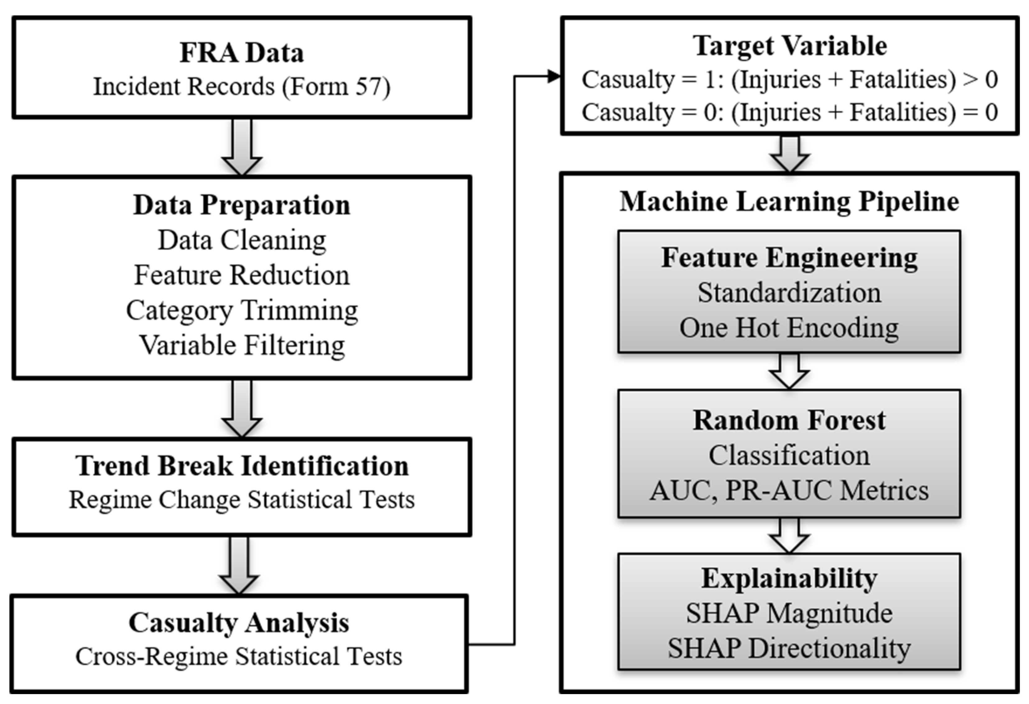
Figure 2.
Results of the regime-transition breakpoint analysis of HRGC incidents.
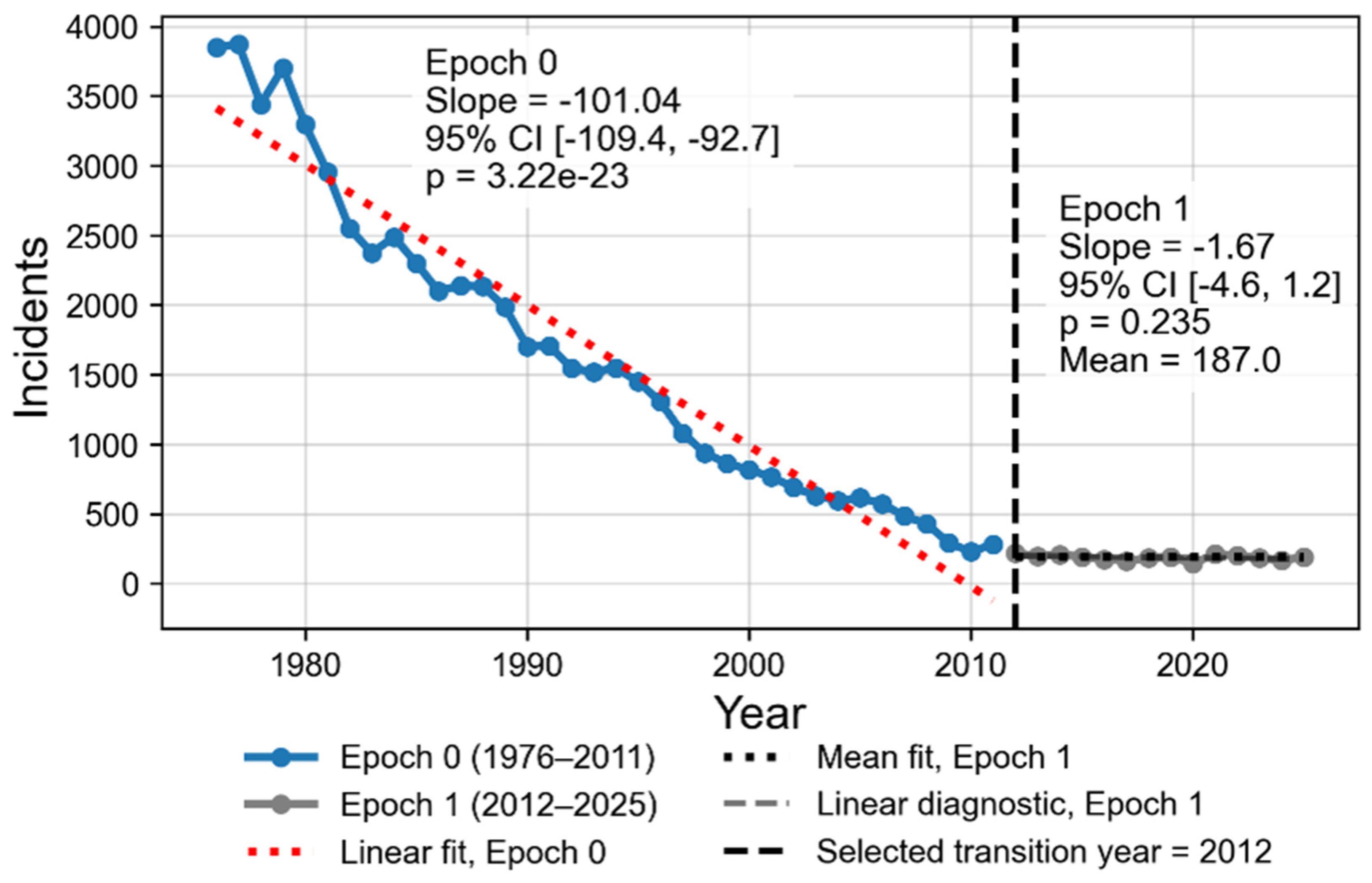
Figure 3.
Comparison of casualty outcomes between Epoch 0 (declining regime) and Epoch 1 (plateau regime). Panel (A) compares the proportion of incidents resulting in at least one casualty. Panel (B) compares the distribution of non-casualty, injury, and fatality outcomes. Insets summarize the corresponding statistical diagnostics.
Figure 3.
Comparison of casualty outcomes between Epoch 0 (declining regime) and Epoch 1 (plateau regime). Panel (A) compares the proportion of incidents resulting in at least one casualty. Panel (B) compares the distribution of non-casualty, injury, and fatality outcomes. Insets summarize the corresponding statistical diagnostics.
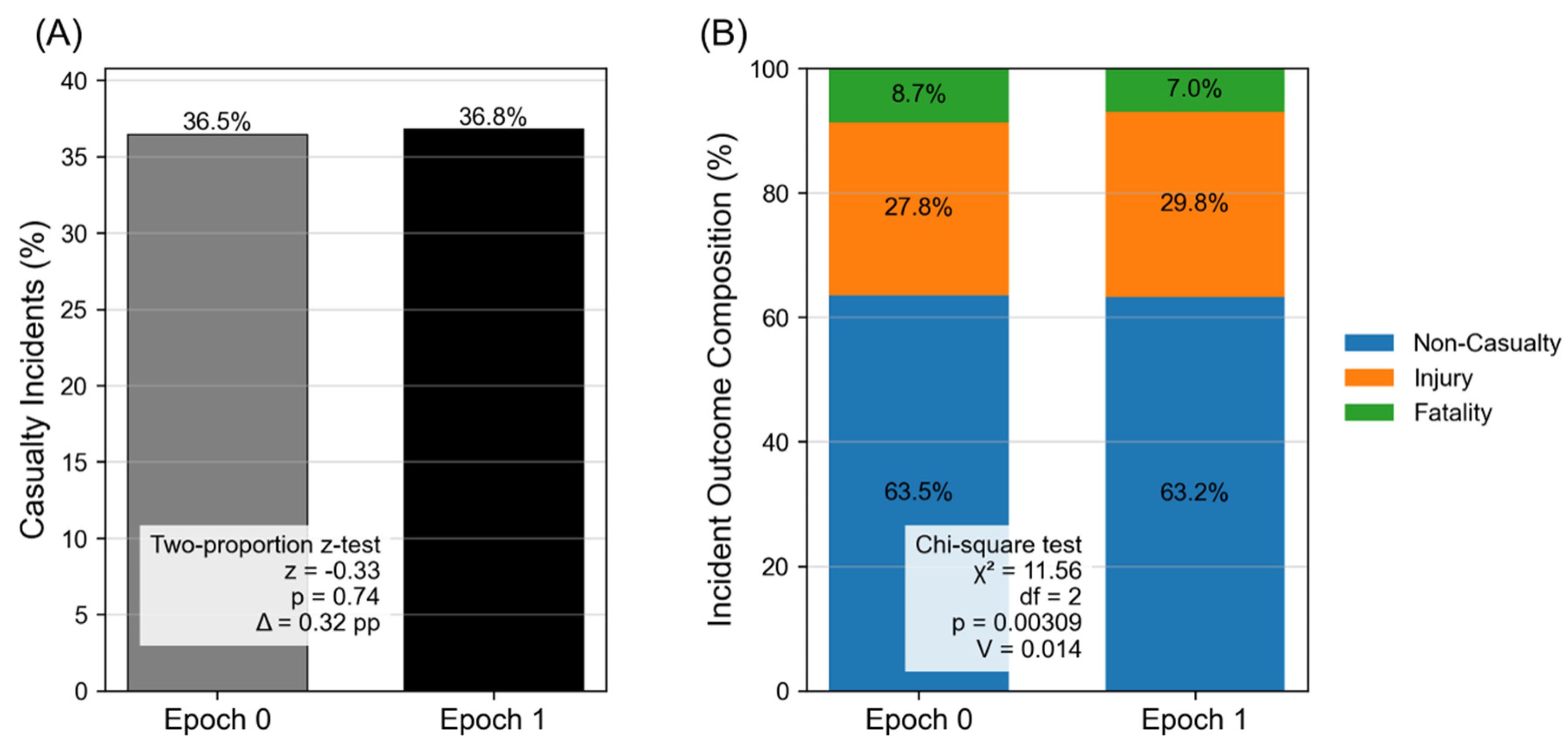
Figure 4.
SHAP importance ranking of numerical and one-hot encoded variables in (A) Epoch 0 and (B) Epoch 1.
Figure 4.
SHAP importance ranking of numerical and one-hot encoded variables in (A) Epoch 0 and (B) Epoch 1.
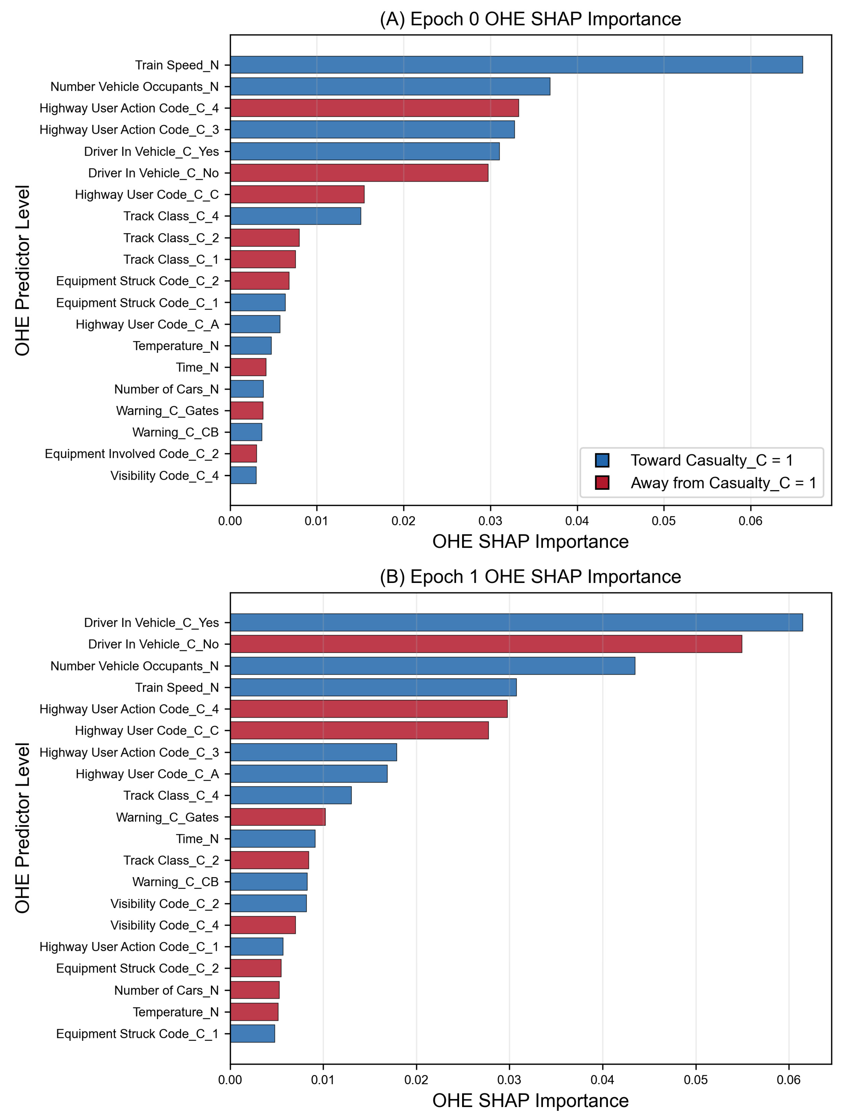

Table 1.
Audit of Data Cleaning Stages.
| Filter | Rows | Columns | Action |
| Original Raw Data | 250,660 | 154 | Loaded FRA Form 57 updated May 13, 2026 |
| Sparsity Filtering | 250,660 | 117 | Dropped >80% missing, add “Row_ID” |
| Public Crossings | 226,499 | 117 | Kept incidents at public crossings |
| HMI/CONUS | 226,094 | 120 | Added reconciled FIP5, Fix_Type, XID |
| Code Label/Meta | 226,094 | 42 | Removed fields with code descriptors and meta data |
| Many Unknown | 226,094 | 39 | Removed fields with too many unknown/missing values |
| Homogeneity Filter | 99,153 | 33 | Class I, freight, mainline, warnings, no obstruction/hazmat |
| Cardinality Trimming | 67,849 | 33 | Remove rows with sparse categories |
| Numerical Filter | 62,011 | 33 | Remove rows with extreme/unlikely values |
| Missing Values | 61,858 | 33 | Remove rows with final missing values |
| Correlated Variables | 61,858 | 31 | Removed two correlated categorical variables |
| Redundant Variables | 61,858 | 29 | Removed Year and Epoch as redundant variables |
| Replacements | 61,858 | 28 | Kept Meta: 7, Categorical: 14, Numeric: 7 |
Table 2.
Audit of Fields Dropped After Homogeneity Filtering. M = missing, M% = missing percentage, C = categories retained, D = rows dropped, %K = percentage of rows kept.
Table 2.
Audit of Fields Dropped After Homogeneity Filtering. M = missing, M% = missing percentage, C = categories retained, D = rows dropped, %K = percentage of rows kept.
| Fields Dropped After Filtering | M | M% | C | D | %K | Dominant |
| Railroad Type | 13 | 0.01 | 1, 1L, 1S | 36,448 | 83.88 | Class 1 |
| Equipment Type Code | 463 | 0.21 | 1 | 48,003 | 74.69 | Freight train |
| Track Type Code | 221 | 0.10 | 1 | 7,387 | 94.79 | Mainline |
| Hazmat Involvement Code | 353 | 0.16 | 4 | 20,319 | 84.87 | Neither rail nor road |
| Crossing Warning Location Code | 2,203 | 0.97 | 1 | 7,748 | 93.20 | Both sides |
| View Obstruction Code | 238 | 0.11 | 8 | 7,036 | 93.37 | Not obstructed |
Table 3.
Audit of Fields Kept After Cardinality Trimming and Numerical Filtering. M = Missing, M% = missing percentage, C/R = categories/range retained, D = rows dropped, %K = percentage of rows kept.
Table 3.
Audit of Fields Kept After Cardinality Trimming and Numerical Filtering. M = Missing, M% = missing percentage, C/R = categories/range retained, D = rows dropped, %K = percentage of rows kept.
| Fields Kept | M | M% | C/R | D | %K | Action |
| Casualty | 0 | 0 | [0, 1] | 0 | 100.0 | “1” if killed/injured > 0 |
| Warning | 3 | <0.01 | [1, 2–3, 7] | 3 | >99 | [Gates, FLS, CB], Other |
| Track Class | 3,398 | 1.5 | 1, 2, 3, 4 | 4,248 | 95.5 | Dropped [0, 5-9, N, O, X] |
| Driver Passed Vehicle | 5,487 | 2.4 | No, Yes | 6,048 | 92.1 | Dropped [Unknown] |
| Equipment Involved Code | 5 | <0.01 | 1, 2 | 1,862 | 97.9 | [Train-Pull, Train-Push] |
| Equipment Struck Code | 5 | <0.01 | 1, 2 | 0 | 100.0 | [RR Struck User, User Struck RR] |
| Highway User Action Code | 3,003 | 1.3 | 1, 2, 3, 4 | 3,971 | 95.1 | [Bypassed, Stop-Move, Moving, Stopped] |
| Highway User Code | 7 | <0.01 | A, B, C, D | 5,997 | 93.1 | [Auto, Truck, Trailer, Pickup] |
| Highway User Position Code | 378 | 0.2 | 1, 2, 3 | 449 | 99.4 | [Stalled, Stopped, Moving] |
| Train Direction Code | 929 | 0.4 | 1, 2, 3, 4 | 72 | 99.9 | [North, South, East, West] |
| Vehicle Direction Code | 1,551 | 0.7 | 1, 2, 3, 4 | 538 | 99.4 | [North, South, East, West] |
| Visibility Code | 17 | <0.01 | 2, 4 | 4,518 | 93.2 | [Day, Dark] |
| Weather Condition Code | 127 | 0.1 | 1, 2, 3 | 3,601 | 94.9 | [Clear, Cloudy, Rain] |
| Driver Condition Code | 6,508 | 2.9 | Missing | 138 | 99.8 | Drop missing values |
| Driver In Vehicle | 5,848 | 2.6 | Missing | 15 | 100.0 | Drop missing values |
| Year | 0 | <0.01 | [1976, 2025] | 5,519 | 94.4 | Dropped 1975, 2026 |
| Number of Cars | 49 | <0.01 | [0, 300] | 2 | 100.0 | Numerical filtering |
| Number of Locomotive Units | 13 | <0.01 | [0, 50] | 1 | 100.0 | Numerical filtering |
| Number Vehicle Occupants | 196 | 0.1 | [0, 100] | 34 | 99.9 | Numerical filtering |
| Railroad Car Unit Position | 1,208 | 0.5 | [0, 300] | 179 | 99.7 | Numerical filtering |
| Temperature (°F) | 1 | <0.01 | [-40, 116] | 2 | 100.0 | Numerical filtering |
| Time (24-hour numeric) | 26 | <0.01 | [0, 2, 359] | 9 | 100.0 | Numerical filtering |
| Train Speed | 2,406 | 1.1 | [0, 110] | 92 | 99.9 | Numerical filtering |
| Day | 0 | 0 | Retained | 0 | 0 | No filtering required |
| Month | 0 | 0 | Retained | 0 | 0 | No filtering required |
Table 4.
Summary of the Statistical Diagnostics for the 2012 Transition Year.
| Diagnostic | Statistic | p-value | Null Hypothesis (H0) | Decision |
| Epoch 0 (1976–2011) Slope | −101.04 | 3.22×10⁻²³ | Slope = 0 | Reject H0 |
| Epoch 0 95% CI | [−109.4, −92.7] | — | — | — |
| Epoch 1 (2012–2025) Slope | −1.67 | 0.235 | Slope = 0 | Fail to reject H0 |
| Epoch 1 95% CI | [−4.6, 1.2] | — | — | — |
| KPSS Stationarity Diagnostic | 0.089 | 0.10 | Series is stationary | Fail to reject H0 |
| ADF Unit-Root Diagnostic | -5.45 | 1.60×10⁻⁴ | Has a unit root | Reject H0 |
| Ljung–Box Residual Diagnostic | 0.036 | 0.985 | Independently distributed | Fail to reject H0 |
| Minimum AIC | 487.056 (2012) | — | — | 2012 selected |
| Minimum BIC | 490.862 (2012) | — | — | 2012 selected |
| Buffer Sensitivity | 0 | — | — | No years removed |
Table 5.
Cross-validated RF Performance by Safety Regime.
| Metric | Epoch 0 | Epoch 1 |
| Incident records | 59,240 | 2,618 |
| Candidate predictors | 21 | 21 |
| Numerical predictors | 7 | 7 |
| Categorical predictors | 14 | 14 |
| One-hot encoded predictor levels | 88 | 87 |
| ROC-AUC Mean | 0.765 | 0.803 |
| ROC-AUC Standard Deviation | 0.007 | 0.015 |
| PR-AUC Mean | 0.615 | 0.669 |
| PR-AUC Standard Deviation | 0.011 | 0.032 |
| Accuracy Mean | 0.677 | 0.709 |
| Accuracy Standard Deviation | 0.006 | 0.010 |
Disclaimer/Publisher’s Note: The statements, opinions and data contained in all publications are solely those of the individual author(s) and contributor(s) and not of MDPI and/or the editor(s). MDPI and/or the editor(s) disclaim responsibility for any injury to people or property resulting from any ideas, methods, instructions or products referred to in the content. |
© 2026 by the authors. Licensee MDPI, Basel, Switzerland. This article is an open access article distributed under the terms and conditions of the Creative Commons Attribution (CC BY) license (http://creativecommons.org/licenses/by/4.0/).
Copyright: This open access article is published under a Creative Commons CC BY 4.0 license, which permit the free download, distribution, and reuse, provided that the author and preprint are cited in any reuse.


