

Submitted:
06 July 2026
Posted:
07 July 2026
You are already at the latest version
Abstract
Poorly governed geoscience databases introduce subtle but systematic biases that propagate through mineral resource estimation workflows, distorting grade continuity and resource classification. While the importance of data quality in mining is widely acknowledged, quantitative demonstrations of how specific data-management decisions translate into downstream technical and economic impacts remain limited. This study addresses that gap through three case studies derived from real-world industry examples. The first case study quantifies operator-dependent data extraction bias by comparing two independently generated datasets sourced from the same database on the same day. Despite nominal equivalence, the datasets differed materially in record counts and grade distributions, producing only negligible global volumetric differences (~0.1%) but up to ~5% local geometric variability and a 19.5% difference in estimated copper grade, resulting in a ~36% divergence in projected revenue. The second case study evaluates analytical uncertainty near detection limits using duplicate assay pairs, demonstrating that relative error increases markedly at low concentrations and that this behavior reflects inherent analytical limitations rather than laboratory non-compliance. The third case study examines the common practice of assigning detection-limit placeholder values to un-assayed intervals, showing that such substitutions can artificially generate ore in barren domains, whereas retaining null values and applying assignments during post-processing yields geologically and statistically coherent results. Collectively, these case studies demonstrate that hidden data biases can exert a stronger influence on resource outcomes than estimation methodology alone. The results highlight the need for standardized extraction workflows, explicit treatment of low-grade uncertainty, and validation practices that extend beyond global reconciliation metrics. Robust data governance and transparent, reproducible workflows are essential to reducing compounding uncertainty and improving confidence in mineral resource models. All datasets have been anonymized, scaled, or modified to prevent identification of any specific project, company, or operation. No confidential or propriety datasets are disclosed.
Keywords:
mineral resource estimation
; data extraction bias
; detection limits
; data governance
; uncertainty management
1. Introduction
Effective data management has never been as critical as it is in modern mining operations. Data underpins the entire mining value chain from exploration to closure, and vulnerabilities in its quality or integrity can compromise this entire system. For industries that rely heavily on data, such as mining, treating data as a core asset is essential. Not only is it important, but with the increase in scale of mining operations, the complexity of geology on ore deposits, more data is generated and required every day. Billion-dollar decisions depend on such databases and, even subtle biases or inconsistencies within the data can propagate through modeling workflows, forecasts, and strategies. These have effects that extend beyond technical metrics and ultimately will determine project viability and profitability. Furthermore, the implications are not confined to statistical analysis. Flawed data introduces uncertainty [1], which can contribute to operational and psychological stress, affecting personnel well-being, workplace relationships and dynamics. Beyond technical impacts, broader consequences of data quality failure have been noted in the literature, including operational risk and occupational health [2]. Therefore, standard protocol and software is necessary to effectively manage such an important component of the mining operation [3]. Despite its critical role, data is often collected under inconsistent protocols, stored with minimal governance, and manipulated by assumptions rather than standards. The longstanding principal “garbage in, garbage out” remains valid. The cumulative effect is the emergence of undetected errors that undermine confidence, increase risk, and influences outcomes across all stages of the mining process.
In mining, mineral resource estimation is a cornerstone of project evaluation and overall feasibility. A robust and well- constructed resource model depends on strong data integrity. Poorly governed databases can distort geological interpretations and lead to flawed conclusions, ultimately impacting project economics and decision-making.
Effective database management requires a combination of automated quality control checks and validation by a qualified person to ensure data integrity before integration into the resource model. These validations typically include basic quality controls, such as ensuring there are no overlapping intervals, missing assays or geological data, excessive drillhole deviation, collar positions outside topography, or invalid assay values (e.g., zero or negative).
In large or complex operations, additional errors often arise when governance controls, extraction logic, and unit consistency are not clearly defined or enforced. This underscores the need for rigorous data management practices to safeguard the reliability and reproducibility of resource estimates.
Ultimately, resource estimation is potentially less influenced by the choice of estimation methods than by systematic, poorly documented database issues that introduce bias, instability, and irreproducibility. These problems are common, frequently legacy-driven, and often remain undetected until the reporting stage. [4] propose a reflective exercise, encouraging practitioners to evaluate their database quality by answering five key questions:
- How much data do you have?
- What is the cost of replacing each data point?
- What is the collective value of the data?
- How much data remains unused?
- How much data is unfit for use?
This simple exercise provides a framework for assessing data quality and determining the cost implications of poor data integrity. It also helps to target improvement initiatives and efficient allocation of resources.
In addition to these retrospective questions, a few forward-looking considerations can further strengthen long-term data governance:
- In what ways can current data collection practices influence information interpretation, relevance and utility in 5, 10 and 20 years?
- To what extent might future practitioners identify gaps in the data that is or is not collected, stored and verified today?
- What is the scope and effectiveness of the current data acquisition process and its oversight?
The forward-looking questions put the data quality assurance in another perspective, not as retrospective exercise but a proactive responsibility. Current data collection actively shapes how information will be interpreted and relied upon in the future. Decisions made today about data storage, validation, and sampling protocols will determine whether data remains comparable and meaningful over time. Moreover, existing gaps on the database and its governance may only become apparent years down the line, when future practitioners attempt to reinterpret or reprocess the data under new economic and technical contexts. This can be a costly rework, introducing uncertainty and even limiting the ability to update resource models. Finally, scoping the effectiveness of data acquisition will define the level of confidence that can be placed in downstream applications, from geological interpretation to resource estimation and mine planning. Having this responsible outlook on data rather than reactive actions places database governance under a strategic function that anticipates future use cases and technological advancements.
This standpoint aligns with [5] who discusses how the perception of data management must inevitably change within the mining industry. With the advances made in technology, companies are collecting and have the potential to collect even more data in real time. Fast and reliable data analysis will be pivotal and can potentially change the whole operation landscape.
Rather than reiterating general principles of data quality, this study provides quantitative, end-to-end evidence of how specific, routinely applied data-management decisions alter geological models, estimation behavior, and economic outcomes. Using three industry-based case studies it isolates distinct bias mechanisms, demonstrating how operator- based decisions, analytical behavior near detection limits and treatment of un-assayed intervals, propagate through the workflow and influence the reliability of model outputs. The results herein presented show that seemingly minor upstream database choices can produce locally significant geometric changes, order of magnitude differences in grade uncertainty and economically material divergences in resource outcomes, even when global reconciliation metrics appear stable.
2. Materials and Methods
This study adopts a case-study-based approach to examine how different sources of hidden bias arise and propagate within mineral resource databases and downstream modelling workflows. A case-study framework was selected because it allows end-to-end evaluation of operational decisions, capturing interactions between data management, geological interpretation, geostatistical analysis, and economic outcomes that are difficult to isolate in synthetic examples. The three case studies were intentionally selected to represent distinct and commonly encountered bias mechanisms: (1) operator-dependent data extraction from a shared source database, (2) analytical uncertainty associated with assays near detection limits, and (3) the treatment of un-assayed or geologically barren intervals through assigned placeholder values versus null handling. Together, these cases span database construction, analytical measurement, and estimation workflow decisions. Across the studies, standard industry tools and methods are applied consistently to reflect realistic practice. Geological interpretations are developed using Leapfrog® software. Statistical and distributional analyses included descriptive statistics, histograms, cumulative probability plots, and Bland–Altman analysis for paired assay comparisons. Resource estimation sensitivity was evaluated using inverse distance cubed (ID³) interpolation and, where appropriate, ordinary kriging to assess the geostatistical implications of dataset differences.
2.1. Case Study 1
Consider a database for a skarn deposit. In the early stages of the resource reporting process, the assay database is validated by the geologist, which is the primary input for estimating tonnage, grade and contained metal in the resource model. These outputs form the basis for investment decisions, mine planning and life-of-mine assessments. Because these decisions depend directly on the data analysis results, maintaining rigorous data integrity is critical.
To exemplify, consider a common issue observed across industry databases. Independent data extractions provided to resource teams can differ depending on the methods and assumptions applied. Initial review often shows that different extraction approaches result in significantly different versions of the same database, as shown in Table 1.
From Table 1, the discrepancies between the datasets are clear. Data 1 contains 8% more drillholes than Data 2. The number of 10-ft composites varies widely. Most concerning, however, is the variation in average copper grade; in which Data 1 presents a 9% lower average grade than Data 2. While the data pertains to the same deposit and same company, without standardized extraction procedures and thorough database vetting, downstream users are likely to model entirely different interpretations of the same deposit.
Moreover, the data obtained also presented mismatches on the lithology log interpretation column. While Data 1 had all intervals with assigned lithology, Data 2 had null values. This is another factor that can impact the understanding of the subsurface. Table 2 presents the differences on the different lithology extracted with the same drill hole ids. This may be due to priorities defined during the extraction process, leading to different outputs from the database.
Moreover, the database also presented differences in sample grade values. That is, at the same interval, same drillhole id, as shown in Table 3. Although both data extractions were performed with the same stated objective, from the same underlying database, the results reveal a clear operator-depending extraction bias. Despite identical intent, differences in how extraction rules were interpreted and implemented resulted in non-equivalent datasets. The observed discrepancies are therefore systematic rather than random and cannot be attributed to geological interpretation, sampling density or estimation methodology.
2.1.1. Geologic Model Differences Arising from Operator Dependent Extraction Bias
Table 2 demonstrates significant discrepancies between Lith Data 1 and Lith Data 2. This mismatch is unexpected, particularly because the drillholes in question are older and therefore their geological information should already exist in the database, with the extraction dates being the same with the two datasets. The failure to correctly extract lithological data has substantial implications for downstream geological and resource-modelling workflows. In Seequent’s Leapfrog® software, lithological intervals form the basis for automatically generated geological models; any errors in the lithology column, or in derived interpreted fields, directly propagate into the modelling process. Although the geology model used to inform the Mineral Resource estimate typically undergoes rigorous validation, automatically generated operational or production models are often updated frequently and may not receive the same level of scrutiny. Consequently, deficiencies in lithological inputs can lead to major domain instabilities, which in turn can produce substantial variability in grade estimation outcomes and orebody distribution. Ensuring the integrity and consistency of lithological data is therefore critical to maintaining the reliability of both interpretive and automated modelling frameworks.
Leapfrog models were constructed using identical workflows (i.e., the same modeling code and column settings). Geologic interpretations for datasets 1 and 2 are generated with the Geologic Model function and explicitly incorporate the intrusion depicted in Figure 1.
2.1.2. Results Case Study 1
At the district/structural scale, the resulting geometries are broadly concordant; however, systematic discrepancies emerge at the local scale. As illustrated in Figure 1, these deviations are spatially localized and manifest as small, distributed zones of both gains and losses. Volumetric reconciliation seen in Table 5 indicates a 5.4% gain and a 5.3% loss when comparing the two surfaces, yielding a negligible net volumetric change of ~0.1%.

Table 4.
Volume comparison of geologic unit created by Data 1 and Data 2.
| Dataset | Data 1 | Data 2 | Difference | % Difference |
|---|---|---|---|---|
| Volume | 73,227,152,049 | 73,294,745,747 | (67,593,698) | 0.09% |
Table 5.
Gains and losses from Data 1 geologic model to Data 2 model.
| Dataset | Gain 1 to 2 | Loss 1 to 2 |
|---|---|---|
| Volume | 3,930,121,253 | 3,862,527,521 |
| Difference in volume from data 1 | 5.4% | 5.3% |
The near-zero net volume change suggests that global inventory is stable; however, the paired 5.4%/5.3% bidirectional differences indicate material local uncertainty. In practice, this is consistent with edge effects at lithological contacts (particularly along the intrusion-host rock boundary), scale-dependent smoothing, and sensitivity to sparse or clustered data supports in structurally complex zones [6,7].
While the overall volumetric balance is effectively unchanged, local geometric differences can influence domain coding, compositing boundaries, and variogram stationarity—ultimately affecting grade interpolation (i.e., kriging) and local selectivity. Effects will be most pronounced in narrow or high-gradient zones where coding differences shift samples across domains.
A 0.1% net volume change is below typical materiality thresholds for global resource statements; however, the ~5% local swing indicates a non-trivial redistribution of volume that may be material for mine design features (e.g., stope outlines, dilution envelopes) and reconciliation at the bench or panel scale.
To further contextualize the volumetric balance observed between the model extracts, statistical summaries and histogram analyses of the raw assays in the modeled geologic units from Data 1 and Data 2 are examined (Figure 2 and Table 6).
Despite the near-constant total modeled volume, the statistical comparison reveals substantial divergence in the underlying sample populations. The number of assays assigned to the modeled unit decreases by 68% from Data 1 to Data 2, while the mean grade increases by 18% and the coefficient of variation (CV) decreases by 36%. These pronounced differences indicate that the two datasets do not represent equivalent populations, highlighting inconsistency in extraction and underscoring the practical consequences of applying unclear or non-standardized rules.
The divergence is further reflected in the distributional form. Data 2 exhibits a pronounced bimodal distribution with a CV exceeding 2, indicating a highly variable distribution and potential violation of the stationarity assumption required for ordinary kriging, and therefore its use is compromised. This can lead to increased smoothing of estimated and reduced local accuracy [8,9]. Also, this behavior suggests that the domain may be aggregating multiple geological populations, warranting further discussion with the geologist regarding the need for re-domaining or sub-domaining to restore stationarity.
In contrast, Data 1 displays a right-skewed but unimodal distribution with a comparatively lower CV. While still heterogeneous, the degree of variability remains within a range that is commonly accepted for the application of ordinary kriging, provided that appropriate variogram modeling and top-cut strategies are employed. As such, Data 1 more closely satisfies the theoretical assumptions of stationarity required for conventional geostatistical estimation [10,11].
The observed changes in CV and tail behavior imply materially different stationarity and variogram characteristics [12], which directly influence kriging performance, local selectivity, and grade smoothing.
Consequently, even though the global volumetric balance is stable, the distributional shifts are material at the local scale, particularly at the stope or drift level. These results demonstrate that volumetric reconciliation alone is insufficient for model validation and that statistical and distributional diagnostics are essential for assessing the geological and geostatistical validity of alternative interpretations.
2.1.3. Estimation Differences
To further assess the potential downstream impact of uncertainty associated with the extraction methodology, an inverse distance cubed (ID³) estimate was completed as a comparative exercise. The ID³ estimation employed a large isotropic search radius of 1,300 ft, with a minimum and maximum of 4 and 18 informing samples, respectively, and a restriction of no more than three samples per drillhole.
Variogram analysis was attempted; however, a stable and interpretable variogram model could not be developed. As a result, an omnidirectional experimental variogram was generated and used solely to inform the selection of an appropriate search distance for the ID³ estimation.
The estimation results are summarized in Table 7. Both datasets were evaluated above a cutoff grade of 0% Cu. A generic bulk density, provided by the site team, was applied consistently to both datasets to ensure comparable and reasonably accurate tonnage estimates.
The comparison highlights meaningful differences between the two datasets. Data 2 reports a 19.5% higher copper grade relative to Data 1, while total tonnage is 12.0% lower. Despite the reduction in tonnage, the higher grade in Data 2 results in an overall 5.1% increase in contained copper metal. These results illustrate that grade variability exerts a stronger influence on contained metal than tonnage alone and underscores the sensitivity of resource outcomes to input data selection. Also, it is important to highlight that density variability potentially amplifies this result.
Visual differences between the two estimates, including the spatial distribution of grade are illustrated in Figure 3.
2.2. Case Study 2
2.2.1. Historical Context
For many years, persistently low metal prices meant that grades near analytical detection limits were of little economic relevance at many operations and projects. Assays near detection limit were rarely used in key technical or economic decisions and were often treated as dilution, effectively classified as “waste”. In many cases, these low-grade values were commonly ignored, censored or not sampled at all. Where material was logged as “waste”, samples were not submitted for analysis to conserve time, budget and other resources.
Within the economic context of the time, these practices were considered reasonable. The implicit assumption was that analytical performance at very low concentrations was inconsequential since such grades were not anticipated to contribute meaningfully to mine planning, reconciliation or value determination.
2.2.2. Shift in Economic Relevance
As commodity prices increased, many mines and projects began operating and conducting technical studies within grade ranges that were never intended for detailed evaluation. Material once dismissed as “background noise” has become potential ore under today’s economic assumptions.
This shift exposed a previously hidden bias in the resource database. Analytical precision at low concentrations was far poorer than assumed by the company or operational side and historical low-grade values no longer supported the accuracy required for modern mine planning and reconciliation. While laboratories have long documented that analytical precision degrades as concentrations approach the detection limits, an expected and well-understood phenomenon, the bias arose because these low-grade ranges were historically irrelevant. As a result, laboratory performance near detection limits was rarely scrutinized, particularly in production sampling.
Consequently, internal mental models, workflows and databases inherited decades of low-grade data that had effectively been neglected yet were later expected to support materially different decisions.
2.2.3. Commodity-Driven Misalignment
An example of where this situation could occur is where copper was the main contributor to project economics, with gold a secondary by-product. Consequently, the testing programs, technical studies and underlying assumptions were designed primarily around copper. As the commodity price increased for gold, the cutoff for gold grade dropped to now include the old and new detection limit assays with the rest of the ore.
2.2.4. Dataset Description
This case study is analyzing assay data from a deposit with low grade gold. A blasthole dataset from riffle splitter sampling method was used and included primary and duplicate assays. A total of 1,610 duplicate assay pairs for gold grade were available for this analysis and presented in Figure 4, providing a robust basis for evaluating analytical precision at concentrations near detection limit.
It is seen in Figure 4 that the distributions seem rather similar in shape and scale, with the Duplicates (Dup) having a slightly higher maximum value for Au than the Original (Orig) and the Original (Orig) having a slightly higher standard deviation than the Duplicates (Dup).
The lower portion of the distribution is the focal point of this study. In Figure 5 it is noted that for gold grades less than 0.01 ounces per short ton (opt), there is negligible bias between Original and Duplicate where the Original is always slightly lower grade than the Duplicate and good reproducibility. The paired scatter fit (Dup = 0.95 Orig + 0.0004 presented in Figure 6; crosses the 1:1 line at around 0.008 opt: duplicates trend slightly higher than originals below this grade and slightly lower above it. Most pairs fall within ±20-30%, consistent with expected low-grade variability.
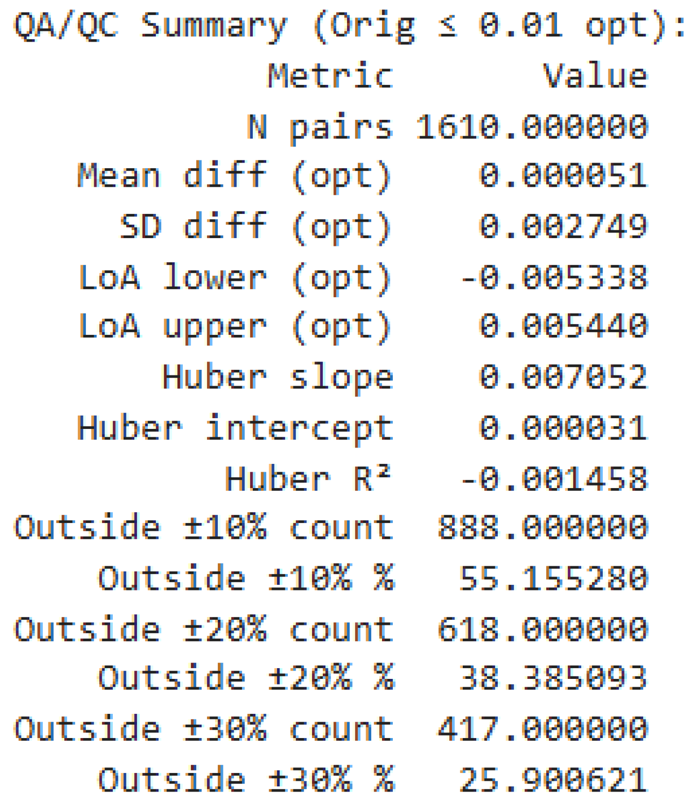
Bland-Altman analysis is used to evaluate agreement between original and riffle duplicate gold assays, focusing on differences rather than on correlation. For samples defined by the Original Au ≤ 0.01 opt, the mean difference is near zero as seen in Figure 8, indicating negligible average bias, with 95% limits of agreement of approximately ±0.0054 opt reflecting expected low-grade analytical variability. A robust Huber regression of difference versus mean shows only a weak, non-explanatory trend (slope ≈ 0.007, ). In percentage terms, ~45% of the pairs lie within ±10% of the mean, ~62% within ±20%, and ~74% within ±30%, consistent with the fact that relative error inflates at very low grades even when absolute difference remains small. Overall, no material systematic bias is evident in the low-grade tail, and precision is fit-for purpose.
Figure 7.
Bland-Altman: duplicate vs. original (orig ≤0.01opt).
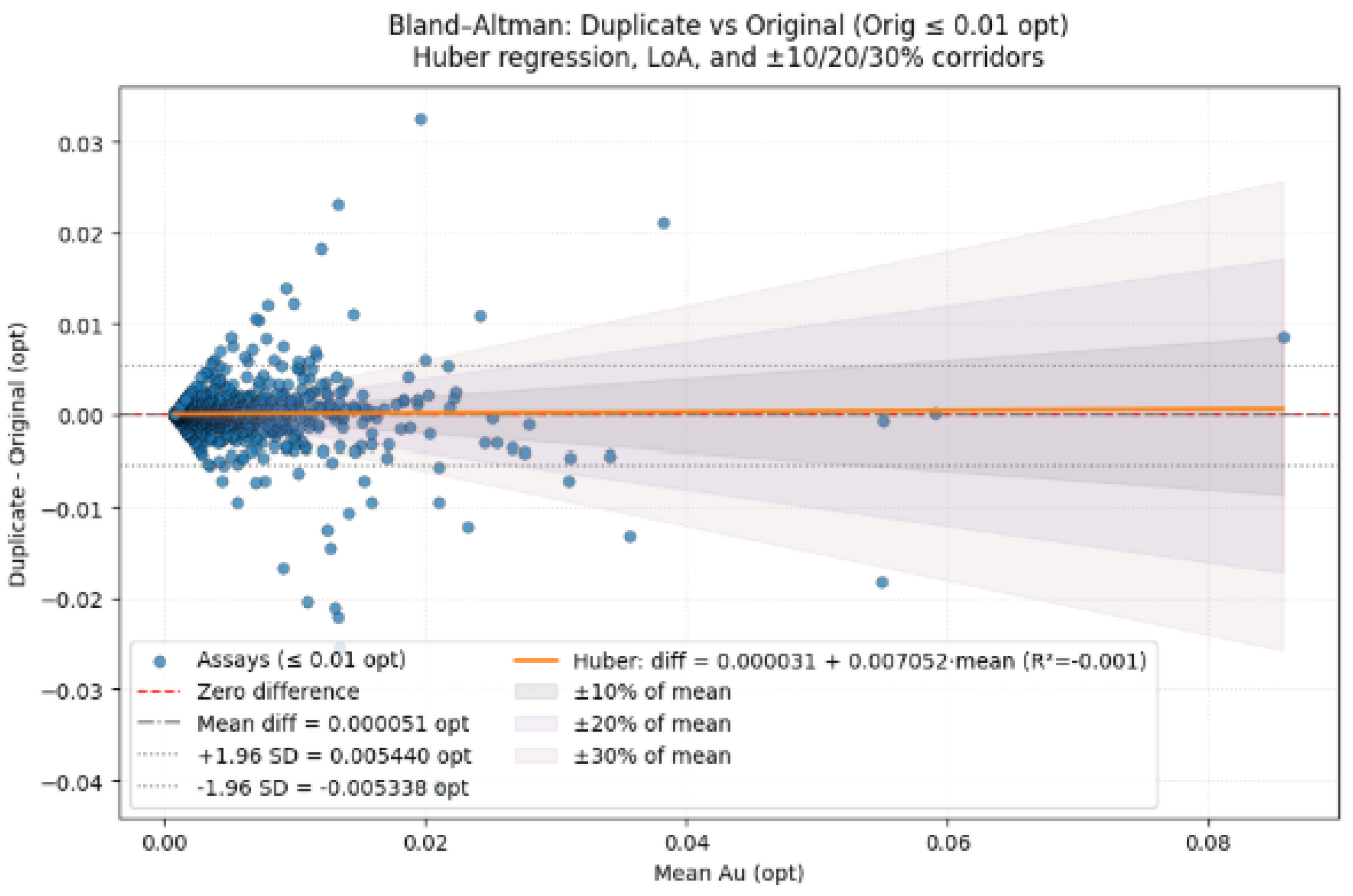
Figure 8.
QA/QC Summary: Duplicate vs original (orig ≤0.01opt).
The cumulative probability plot, paired scatter and Bland-Altman analyses demonstrate negligible average bias between original and riffle duplicate assays and show scatter consistent with expectations at low grades, with relative error inflating as grades approach the detection limit. These analyses, however, do not explicitly describe how laboratory control limits are constructed near the detection limit, nor how this construction can cause an otherwise symmetric error structure to appear biased when expressed in percentage terms. This behavior is often informally attributed to geological nugget effects; however, ALS Global’s QC limits fact sheet “QC Limits Fact Sheet_Rev2.0.pdf”, here taken as an illustrative of a broader analytical principal, makes it clear that it is also an inherent consequence of method precision, detection limits, and reporting increments. ALS explicitly accounts for degraded precision near the detection limit by expanding acceptable control limits through the inclusion of detection-limit-based terms, formalizing the inflation of relative error at very low concentrations as seen in Figure 9.
As stated in the ALS QC Limits Fact Sheet, the basic formula for target performance control limits for analytical reference material is: Conc ± P * Conc where Conc is the concentration of the reference material and P is the precision expectation of the method, and this formula does not accommodate reporting in increments of the detection limit. The calculated limits may be smaller than what is reported analytically. To address this, an adjusted formula is applied to concentrations below 20 times the method’s detection limit, providing an additional margin:
Based on Figure 10, it is evident that as gold concentrations approach the analytical detection limit, the calculated percent difference increases substantially when using the <20x detection limit formulation compared to the basic percent difference formula. The basic formula applies to a constant proportional error, resulting in a uniform ±10% difference across all concentrations. In contrast, the <20x DL formulation explicitly incorporates the detection limit into the calculation, leading to progressively larger relative differences at low concentrations.
For this study, historical gold concentrations are commonly near legacy detection limits. As a result, uncertainty associated with low-grade assays is expected to be elevated, with potential relative differences ranging from approximately ±10% at higher concentrations to greater than ±200% at or near detection limit. These elevated differences reflect the conservative behavior of the <20x DL formulation rather than true analytical precision and are intended to appropriately represent uncertainty in low-level gold data.
2.2.5. Discussion
This case study demonstrates that low-grade gold assays near detection limit can exhibit acceptable precision and negligible systematic bias when evaluated using detection limit appropriate QA/QC frameworks. Apparent inflation of relative error at very low concentrations is shown to be a predictable consequence of analytical method behavior rather than analytical failure. These effects reflect legacy misalignment between historical data collection practices and modern economic requirements.
2.2.6. Implications for Reconciliation and Low-Grade Material Handling
When analytical precision near the detection limit is not the primary driver of reconciliation performance, it represents a subtle but systematic source of uncertainty that can contribute to observed reconciliation differences when low-grade material becomes economically relevant. As demonstrated in this case study, relative error in gold assays inflates at concentrations near the detection limit due to method precision, reporting increments and detection limit-based control limits, even when absolute differences remain small and unbiased.
In historical operating contexts, these low-grade gold values were rarely relied upon for material classification or value determination and therefore did not materially influence reconciliation outcomes. Under current economic conditions, the inclusion of low-grade material near detection limits or even historical detection limits into ore classifications, stockpiles and processing streams introduce a component of variability that was not previously considered. When aggregated over large tonnages, this low-grade analytical variability can manifest as small but persistent differences between model predictions and downstream reconciliations.
This source of uncertainty is not typically represented in resource or reserve models. Standard estimation workflows treat assay values as fixed inputs once composited. When performing simulation workflows, there is uncertainty about data but not for this low-grade near detection limit type data. It’s not separately quantified nor taken into consideration, making its contribution to reconciliation differences difficult to isolate or diagnose.
This does not imply that reconciliation issues can be solely attributed to analytical performance, but it highlights that detection-limit effects represent one of several interacting contributors that collectively influence reconciliation outcomes. Recognizing and contextualizing this effect helps prevent misinterpretation of reconciliation discrepancies and supports more realistic expectations for low-grade material performance.
As progressively lower-grade material is incorporated into mine plans and as and as processing methods advance to enable recovery from these lower-grade materials, analytical uncertainty near the detection limit, increased attention is required for how uncertainty near the detection limit is understood and managed. This does not imply that low-grade data should be arbitrarily adjusted or replaced with detection-limit values or other values, but it highlights the need for explicit acknowledgement of uncertainty in the lower tail whether through conservative reconciliation expectations, sensitivity analysis, domain specific treatment, modifying factors, adjusting the resource classification in these areas or transparent communication of the limitations. This will help with keeping low-grade material from being over-interpreted or unfairly penalized.
2.3. Case Study 3
As stated previously in Case Study 2, there are instances where unmineralized composites are ignored, censored, or not sampled at all. When intervals are logged as unmineralized, these samples are withheld from laboratory analysis to conserve time, budget and other resources. However, that creates gaps in the database where no values are measured for certain intervals. In cases where site geologists are confident that the interval belongs to a barren unit, it is common for these intervals to have values at or near detection limit assigned in database. The reasoning being, there is enough geological confidence that the assigned low values will control and avoid biasing grade upward in locations where there should not be ore; maintain spatial continuity for the estimation step and honor the geological interpretation. Hence, these values are carried forward into resource estimation and classification. Although intended to represent barren intervals, this practice introduces significant technical and compliance risks [14].
In Figure 11 the impact of data handling decisions can be clearly seen on the statistical distribution of the database. On the left histogram, core intervals that are logged as barren lithology are not assayed, and a low–grade of 0.001% Cu is assigned to these intervals. On the histogram on the right, non-assayed intervals are excluded from the analysis. The inclusion of low-grade values introduces a pronounced spike at the lower tail of the distribution and shifts the statistics, thereby distorting the grade distribution relative to the population of measured samples. On the other hand, excluding the non-assayed intervals preserves the natural distribution of assayed grades. This simple comparison demonstrated how the use of background values, even in uneconomical lithologies, can introduce bias that propagated to subsequent geostatistical modeling and resource estimation.
Also, the inclusion of the low–grade values onto the database create an artificial continuity for the grades, as shown in Figure 12.
Figure 12 clearly shows the effect of assigning background values on spatial continuity. The correlograms show that the inclusion of these values consistently results in higher continuity, expressed by a lower decay of the correlation relative to the lag. This behavior smooths the estimates artificially, where low-grade values infill gaps and reduce local variability, effectively masking the natural heterogeneity of the deposit. Consequently, what appears to be improved continuity is not a true geological feature, but a by-product of imposed assumptions on unmeasured data.
For further analysis the two sets of copper grade (Cu) are used for estimation using ordinary kriging, with the corresponding variogram model specific to each dataset. In this context, the kriging parameters are not standardized across databases. As low-grade values are manually assigned to intervals interpreted as barren, serving both to reflect expected geological conditions and to constrain the emergence of unrealistically high-grade estimates in areas where mineralization is not anticipated.
The underlying question is therefore whether the explicit assignment of low-grade values to these intervals the most appropriate approach for is controlling grade behavior, or whether a more restrictive kriging strategy, applied to a database from which such intervals are excluded, would achieve the same objective. Table 10 summarizes the kriging strategy for both cases, labeled as Case 1 (data with assigned low-grade values) and Case 2 (data which exclude non- assayed intervals).
The kriging strategy for was chosen based on optimized estimation parameters for each case. For Case 1, a capping threshold of 1.55% Cu, consistent with the region identified by the red arrow on the red curve. The strategy adopted in Case 2 is to choose an aggressive cap value to restrict the grade inside the domain, preventing inflating estimates.
Therefore, the cap value chosen is 1% Cu, as indicated by the black arrow on the black curve. Combined with the cap, a high yield (HY) search is also applied for samples of 0.8% Cu, allowing one block of influence for those.
Figure 13.
Lognormal probability plots for Case 1 (red curve) and Case 2 (black curve) and chosen cap values in each case.
Figure 13.
Lognormal probability plots for Case 1 (red curve) and Case 2 (black curve) and chosen cap values in each case.
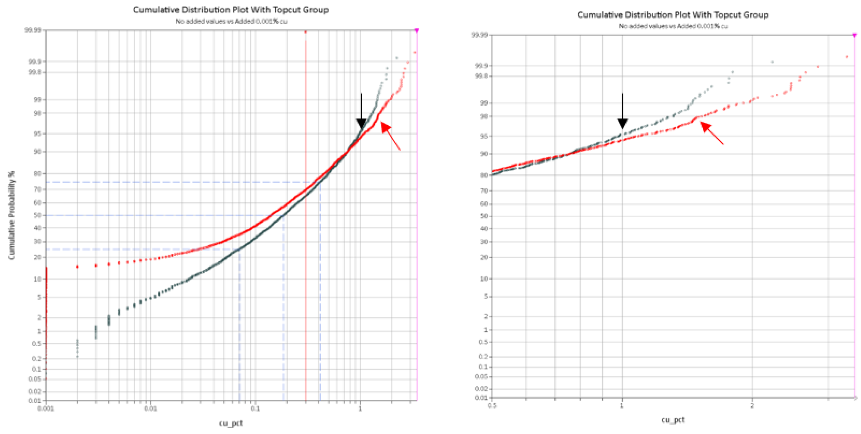
Table 8.
Estimation strategy used on each case considered. Cases consider different strategies due to decisions taken based on the sample database.
Table 8.
Estimation strategy used on each case considered. Cases consider different strategies due to decisions taken based on the sample database.
| Cap. value | HY restriction | Search ellipse | Min num. of samples | Max num. of samples | Num. of samples/dh | |
|---|---|---|---|---|---|---|
| Case 1 | 1.55 | Not applied | 180ft isotropic | 9 | 15 | 3 |
| Case 2 | 1.0 | 0.8 range = 20ft in each direction | 60ft on major; 40ft on semi major and 20ft on minor | 9 | 15 | 3 |
It is acknowledged that the two estimation scenarios evaluated in this case study differ not only in the treatment of un- assayed intervals (assigned placeholder values versus retained nulls), but also in associated estimation parameters such as capping strategy, search geometry, and high-yield restrictions. This coupling is intentional and reflects realistic industry practice rather than an isolated variable test. In operational workflows, the removal of placeholder values fundamentally alters the statistical population and support of the dataset, necessitating corresponding adjustments to estimation controls to maintain geostatistical validity. Treating placeholder removal as a standalone change, while holding all other parameters constant, would misrepresent how practitioners adapt workflows in response to altered data characteristics. Accordingly, the comparison presented here should be interpreted as a workflow-level evaluation, demonstrating how alternative data-handling philosophies propagate through estimation design, model behavior, and resource outcomes under practical conditions.
Added to the different kriging strategy, Case 2 uses post-processing of the un-estimated blocks, assigning to blocks the low-grade value of 0.001% Cu. The databases declustered means are 0.28% for Case 1 and 0.27% for Case 2. The estimates obtained respectively 0.21% and 0.23% average grade. The relative deviation on Case 1 is -25% from the global declustered mean. On Case 2 the relative deviation is -14% from the global declustered mean.
To evaluate the impact that different choices on how to manage un-assayed samples classification is run for both cases. Classification scheme is kept the same for both variables, given that there is not a necessity for the drill hole to be assayed so it can be considered in the classification scheme, if there is enough confidence in the geology of the drill hole. Measured is defined if the average distance between three drill holes is equal or less than 50ft; indicated is defined if the average distance to three drill holes is greater than 50ft and less than 150ft; finally, inferred is defined if the average distance between two holes is less than or equal to 150ft. Computing resources within the area considered has led to the following:
From Table 9 the substitution of non-assayed intervals with the detection limit produced an artificial appearance of conservatism in the resource model. Although it is commonly assumed that assigning low-grade values mitigates the risk of resource overestimation, this assumption did not hold in this case. Despite applying grade capping, the influence of high-grade outliers was not sufficiently constrained, resulting in an inflated estimate of ore tonnage within a geological domain that is known to be barren. Conversely, the model in which non-assayed intervals were left unassigned yielded a completely barren output, consistent with geological expectations and indicating the absence of economically significant mineralization within this domain.
Importantly, this case study does not suggest that low-grade data should be adjusted, censored or replaced with detection-limit values. Instead, it supports the need for explicit acknowledgement of analytical uncertainty in the lower tail of grade distributions. As progressively lower-grade material is incorporated into mine plans, transparent communication of data limitations, conservative reconciliation expectations, sensitivity analyses or domain-specific treatment may be required to prevent over-interpretation of low-grade model outputs.
3. Conclusions
This study demonstrates that bias in mineral resource databases is rarely introduced at a single point and is seldom detectable through conventional validation metrics alone. Instead, bias commonly emerges from a sequence of technically reasonable decisions that interact across data extraction, geological interpretation, statistical treatment, and estimation workflows, allowing uncertainty to propagate in non-linear and often obscured ways.
The first case study shows that operator-dependent data extraction can generate materially different geological models and statistical populations, even when global volumetric reconciliation suggests negligible change. Local-scale lithological inconsistencies, introduced during extraction, were shown to destabilize domains and violate geostatistical assumptions, leading to significant differences in grade, tonnage, and contained metal. These results confirm that volumetric agreement alone is insufficient to validate model equivalence and that local statistical and spatial diagnostics are essential.
The second case study highlights how legacy data practices can become a hidden source of uncertainty as economic conditions evolve. Analytical behavior near detection limits was shown to be consistent with expected laboratory performance rather than systematic bias. The primary risk arises from misinterpretation: when low-grade material becomes economically relevant, relative error near detection limits may be misconstrued as poor data quality or reconciliation failure. Explicit recognition and communication of low-grade analytical uncertainty are therefore critical to avoiding over-interpretation of model outputs.
The third case study demonstrates that assigning values at or near detection limits to un-assayed or barren intervals can distort grade distributions, impose unrealistic continuity, and bias estimation results. Contrary to common assumptions, such substitutions did not reduce risk but instead generated spurious mineralization in geologically barren areas. Retaining null values and applying restrictive, geologically informed estimation controls produced outcomes consistent with geological expectations. The treatment of null values should be deliberate, documented and clearly communicated throughout the value chain.
Collectively, these case studies reveal a unifying theme: upstream data-handling decisions exert a disproportionate influence on downstream estimation outcomes. Once embedded within geological and statistical frameworks, biases are difficult to detect and correct. Robust data governance, transparent and reproducible extraction workflows, and integrated geological, statistical, and estimation validation are therefore essential to maintaining confidence in mineral resource models and the decisions they support.
Author Contributions
All authors contributed equally to this work and have read and agreed to the published version of the manuscript.
Funding
This research received no external funding.
Data availability statement
The data sets used on the current study are not publicly available due to confidentiality requirements.
Disclaimer
The views expressed are those of the authors and do not necessarily reflect those of their employer(s) or client(s). This paper is intended solely for research and educational purposes and should not be relied upon for investment, valuation, or operational decisions. All datasets have been anonymized, scaled, or modified to prevent identification of any specific project, company, or operation. No confidential or propriety datasets are disclosed. This document does not constitute a Mineral Resource or Mineral Reserve disclosure as defined by NI 43-101, JORC or other CRIRSCO-aligned reporting standards. All estimates are illustrative and prepared solely for methodological comparison
Conflicts of Interest
The authors declare that the research was conducted in the absence of any commercial or financial relationship that could be constructed as a potential conflict of interest.
References
- Bovim, A. B.; Morton, K. L. Advanced monitoring of tailings storage facilities and dams to prevent failure: Illustrated with case studies from UK, Africa and South America. In IMWA 2023 – Y Dyfodol | The Future: Proceedings of the International Mine Water Association Conference, July 17–21, 2023, Newport, Wales ; Stanley, P., Wolkersdorfer, C., Wolkersdorfer, K., Eds.; pp. 69–76.
- Matamala Pizarro, J.; Aguayo Fuenzalida, F. Mental health in mine workers: A literature review. Ind. Health 2021, 59(6), 343–370. [Google Scholar] [CrossRef] [PubMed]
- Qi, J.; Wang, P.; Feng, X.; Ma, C.; Su, X. Data standards–based mine-side data integration governance platform: Research and applications. EAI Endorsed Trans. Scalable Inf. Syst. 2024, 11(3). [Google Scholar] [CrossRef]
- Yacopetti, M.; Mundell, S. Improving the quality of geoscientific information. In Proceedings of the Bowen Basin Symposium 2010 – “Back in (the) Black”; Geological Society of Australia, Coal Geology Group and Bowen Basin Geologists Group: Mackay, QLD, 2010; pp. 97–100. [Google Scholar]
- Qi, C.-C. Big data management in the mining industry. Int. J. Miner. Metall. Mater. 2020, 27(2), 131–139. [Google Scholar] [CrossRef]
- Journel, A. G.; Huijbregts, C. J. Mining geostatistics; Academic Press, 1978. [Google Scholar]
- Ortiz, J. M.; Emery, X. Geostatistical estimation of mineral resources with soft geological boundaries: A comparative study. J. South. Afr. Inst. Min. Metall. 2006, 106(8), 577–584. [Google Scholar]
- Goovaerts, P. Geostatistics for natural resources evaluation; Oxford University Press, 1997. [Google Scholar]
- Yamamoto, J. K. Correcting the smoothing effect of ordinary kriging estimates. Math. Geol. 2005, 37(1). [Google Scholar] [CrossRef]
- Matheron, G. Principles of geostatistics. Econ. Geol. 1963, 58(8), 1246–1266. [Google Scholar] [CrossRef]
- Isaaks, E. H.; Srivastava, R. M. An introduction to applied geostatistics; Oxford University Press, 1989. [Google Scholar]
- Chilès, J.-P.; Delfiner, P. Geostatistics: Modeling spatial uncertainty; Wiley, 1999. [Google Scholar]
- ALS Global. (n.d.). Quality control (QC) limits fact sheet (Rev. 2.0). Unpublished technical document. n.d.
- Helsel, D. R. Fabricating data: How substituting values for nondetects can ruin results, and what can be done about it. Chemosphere 2006, 65(11). [Google Scholar] [CrossRef] [PubMed]
Figure 1.
Interpretation of geologic units using Data 1 and Data 2, with the differences.
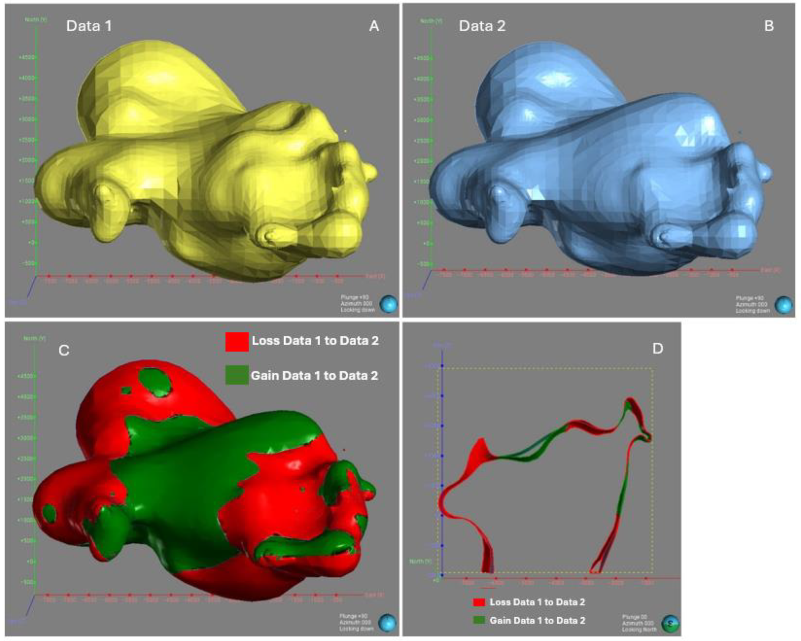
Figure 2.
Raw Cu (%) statistics of each dataset within their respective geologic models.
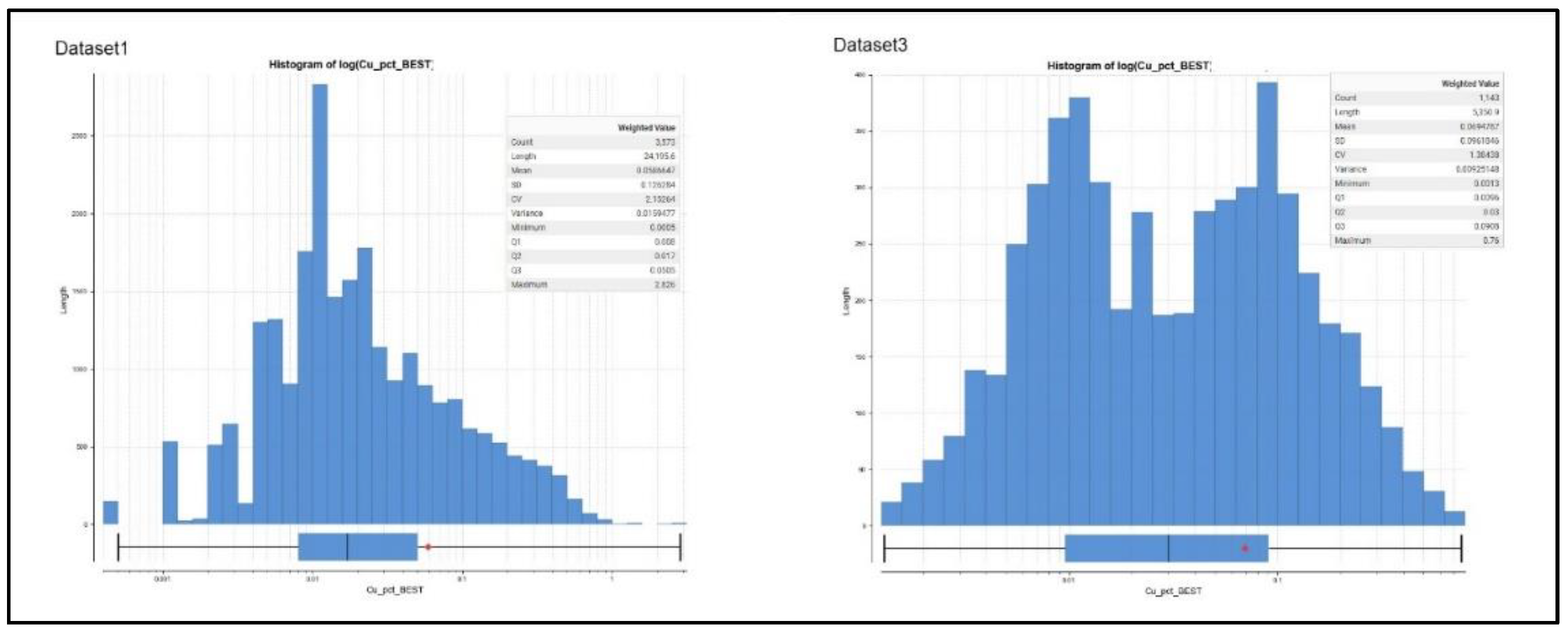
Figure 3.
Differences in estimate between Data 1 and Data 2.
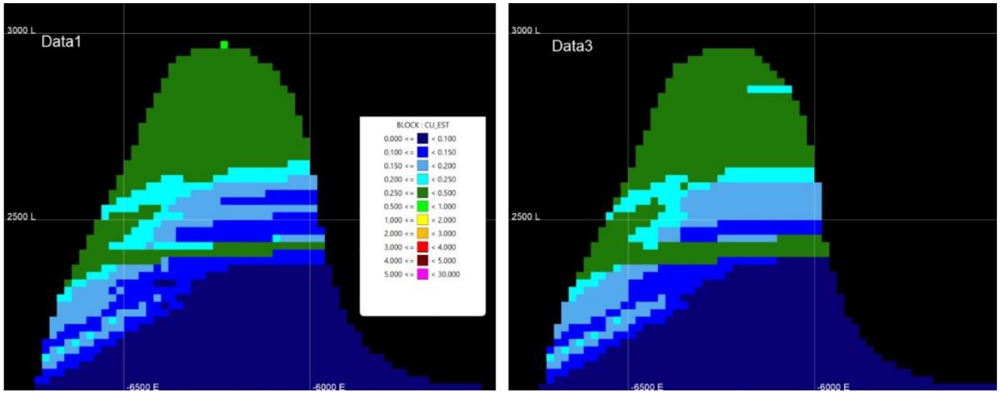
Figure 4.
Overlapping Histogram Plot for Original and Duplicates.
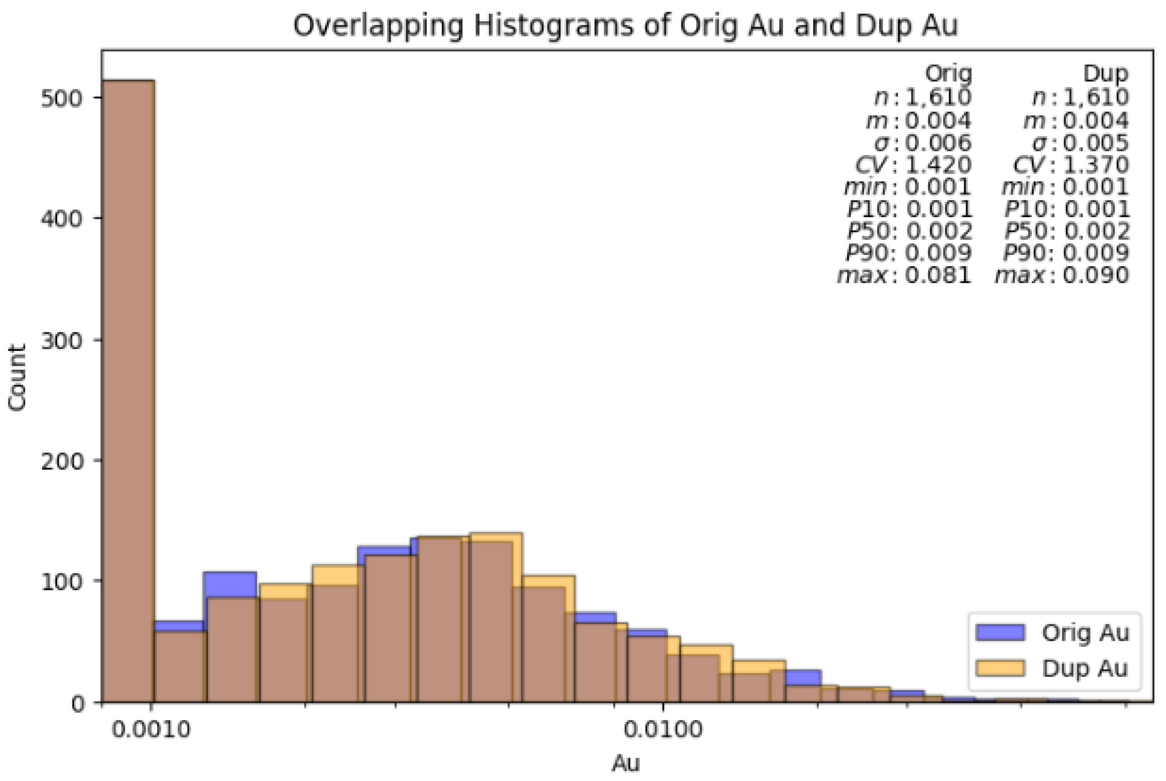
Figure 5.
Cumulative Probability Plot of Original vs. Riffle Duplicate Au Grades.
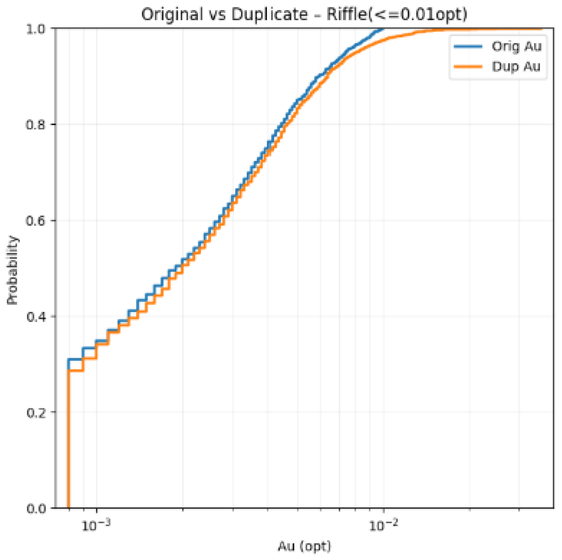
Figure 6.
Paired Scatterplot of Original vs. Riffle Duplicate Au Grades.
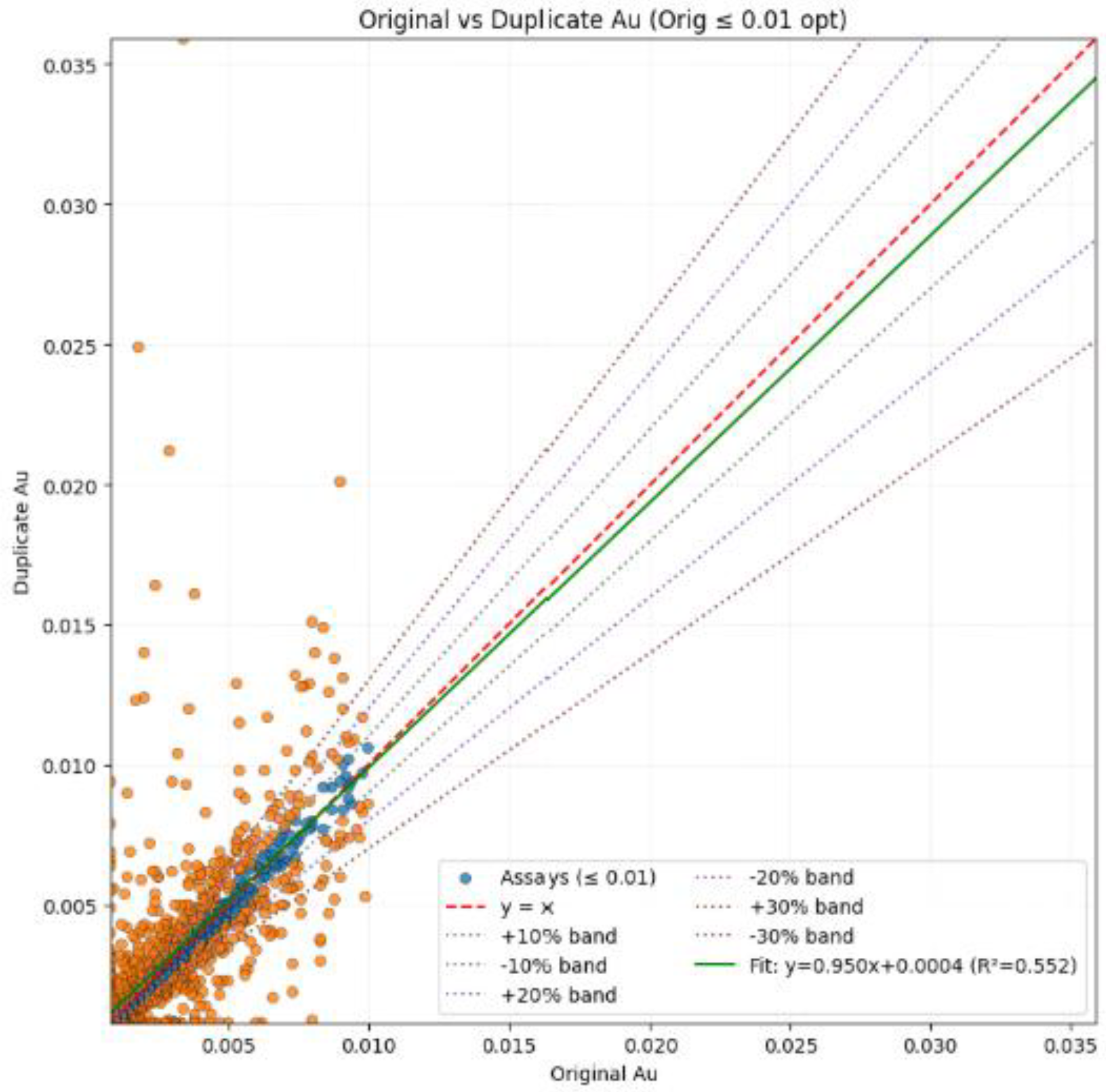
Figure 9.
Percentage precision as a function of detection limit [13].
Figure 9.
Percentage precision as a function of detection limit [13].
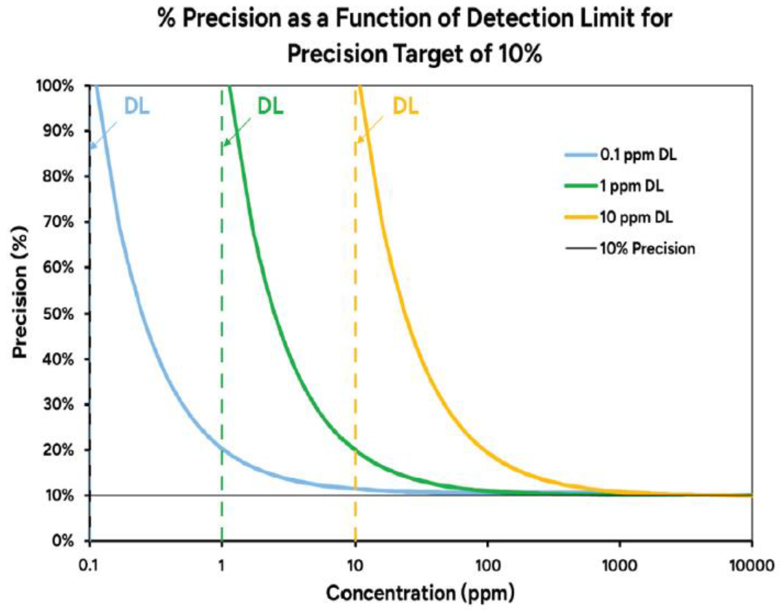
Figure 10.
Comparison of values calculated from both formulas.
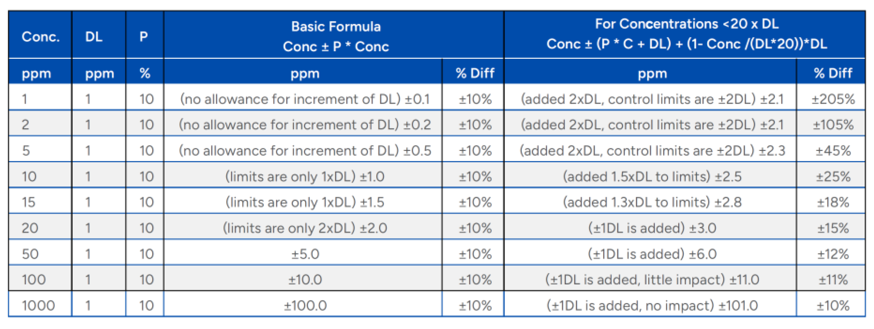
Figure 11.
Lognormal histograms of data with and without assigned grades in non-sampled intervals.
Figure 12.
Variogram with and without the assigned values.
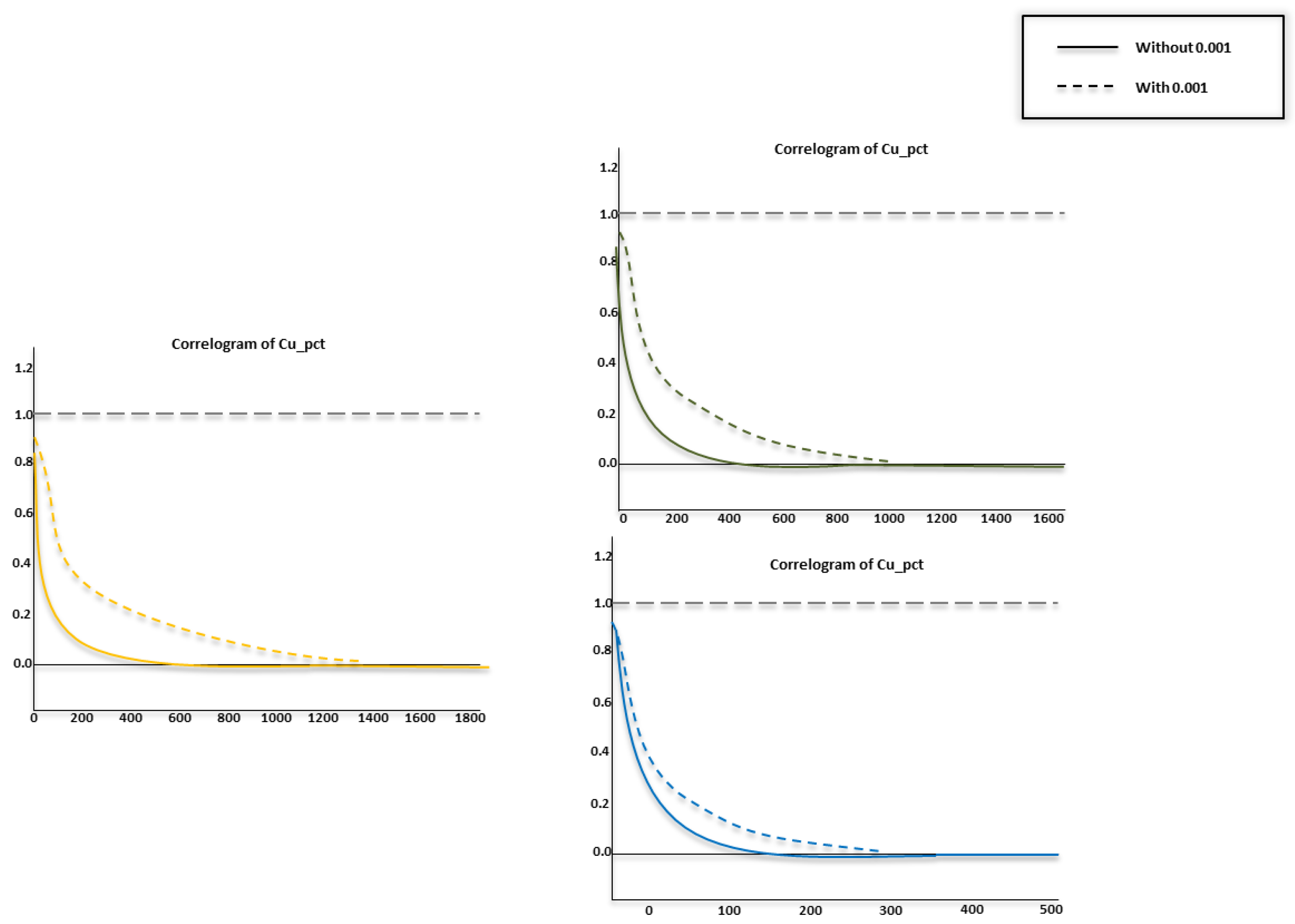
Table 1.
Summary comparison between main metrics on Database 1 and 2.
| Database | Number of drill holes | Number of composites | Average Cu (%) |
|---|---|---|---|
| Data 1 | 404 | 59891 | 0.53 |
| Data 2 | 372 | 32384 | 0.58 |
Table 2.
Comparison between Database 1 and 2 on LITH column extracted.
| DATA | HOLEID | FROM | TO | SAMPLE TYPE | CU (%) | PRIORITY |
|---|---|---|---|---|---|---|
| Data 1 | 1062 | 670 | 675 | NOT IN TABLE | 0.2 | 1 |
| Data 2 | 1062 | 670 | 675 | original | 2.0 | Not in table |
Table 3.
Other differences detected between database 1 and 2 related to copper grade, sample type and priority.
Table 3.
Other differences detected between database 1 and 2 related to copper grade, sample type and priority.
| Hole ID | FROM | TO | LITH Data 1 | LITH Data 2 | |
|---|---|---|---|---|---|
| 10299A | 4385.5 | 4420.0 | nan | quartzite | |
| 10299A | 4420.0 | 4443.0 | nan | quartzite | |
| 10299A | 4443.0 | 4462.0 | nan | quartzite | |
| 10299A | 4462.0 | 4529.5 | nan | quartzite | |
| 10425 | 3040.0 | 3047.0 | nan | monzonite | |
| 10425 | 3047.0 | 3078.2 | nan | monzonite | |
| 10425 | 3079.1 | 3139.0 | nan | monzonite | |
| 10425 | 3139.0 | 3252.7 | nan | monzonite | |
| 10426 | 2418.0 | 2466.0 | nan | skarn | |
| 10426 | 2466.0 | 2469.0 | nan | skarn | |
| 10426 | 2469.0 | 2471.4 | nan | skarn | |
| 10501 | 1921.2 | 1927.0 | nan | quartzite | |
| 10501 | 1927.0 | 1950.0 | nan | quartzite | |
| 10667 | 2750.0 | 2773.0 | nan | skarn | |
| 10667 | 2773.0 | 2774.0 | nan | skarn | |
| 10667 | 2774.0 | 2800.0 | nan | skarn | |
Table 6.
Comparison statistics of raw Cu (%) grade within the interpreted geologic models.
| Data 1 | Data 2 | % Difference | |
|---|---|---|---|
| Count | 3573 | 1143 | -68% |
| Mean | 0.059 | 0.069 | 18% |
| CV | 2.15 | 1.38 | -36% |
| Min | 0.0005 | 0.0013 | 160% |
| Max | 2.826 | 0.76 | -73% |
Table 7.
Estimation results using dataset 1 vs dataset 2.
| Source | Cutoff | Cu (%) | Tons | Cu (lbs) |
|---|---|---|---|---|
| Data 2 | 0 | 0.039453 | 2,425,047,456 | 1,913,525,706 |
| Data 1 | 0 | 0.033013 | 2,756,641,056 | 1,820,082,971 |
| % diff. | 0% | 19.5% | -12.0% | 5.1% |
Table 9.
Results of Case 1 and Case 2 estimation.
| CASE 1 | Class | *Product | Cu (%) | Total Vol. | Total mass | Cu (Lbs) |
| 1 | ore | 1.297 | 108,000 | 296,100 | 384,050 | |
| 1 | waste | 0.245 | 4,677,750 | 12,698,560 | 3,109,029 | |
| 2 | waste | 0.136 | 1,137,375 | 3,086,598 | 418,364 | |
| CASE 2 | 1 | waste | 0.141 | 4,822,875 | 13,096,241 | 1,851,413 |
| 2 | waste | 0.019 | 1,171,125 | 3,178,192 | 60,998 |
*Cuttoff grade is 0.2% Cu. Ore is considered above that threshold in both cases.
Disclaimer/Publisher’s Note: The statements, opinions and data contained in all publications are solely those of the individual author(s) and contributor(s) and not of MDPI and/or the editor(s). MDPI and/or the editor(s) disclaim responsibility for any injury to people or property resulting from any ideas, methods, instructions or products referred to in the content. |
© 2026 by the authors. Licensee MDPI, Basel, Switzerland. This article is an open access article distributed under the terms and conditions of the Creative Commons Attribution (CC BY) license (http://creativecommons.org/licenses/by/4.0/).
Copyright: This open access article is published under a Creative Commons CC BY 4.0 license, which permit the free download, distribution, and reuse, provided that the author and preprint are cited in any reuse.