

Submitted:
03 July 2026
Posted:
07 July 2026
You are already at the latest version
Abstract
We study an effective quantum cosmological model with a scale-dependent gravitational coupling G(a). Starting from a quantum-corrected Newtonian cosmology, we derive a modified Friedmann equation and quantize the corresponding minisuperspace model to obtain a Wheeler–DeWitt equation. For the power-law running G(a)=G0an, the small-scale behavior is controlled by the exponent n. In the flat dust model with a positive quantum correction term Ξ, the values n=3/2 and n=2 mark distinct analytic boundaries: n=3/2 marks the sign change of the quantum-correction coefficient, while n=2 marks the degeneracy of the leading powers of a. A genuine bounce occurs only when a root of H2(a) separates a forbidden small-a region from an allowed expanding branch, so that nonsingular sectors appear without spatial curvature, exotic matter, or nonstandard quantization prescriptions. We obtain Bessel, Airy, numerical, and WKB solutions, and show that the model separates genuine DeWitt suppression from regularity at the origin. The WKB analysis exhibits a forbidden region, a turning point, and an oscillatory semiclassical branch, while the conserved probability current distinguishes expanding and contracting sectors. A scalar-field clock yields wave packets that track the classical trajectory at large scale factor; the WKB Hamilton–Jacobi limit recovers the modified Friedmann dynamics as the leading-order phase of the Wheeler–DeWitt wave function.
Keywords:
quantum cosmology
; Wheeler–DeWitt equation
; running gravitational coupling
; nonsingular cosmology
; cosmological bounce
; minisuperspace quantization
; DeWitt boundary condition
; semiclassical limit
1. Introduction
One of the central questions in quantum cosmology concerns whether the initial singularity of the classical Friedmann picture is an unavoidable feature of cosmological evolution, or whether quantum effects are capable of resolving it. In the standard classical treatment, generic matter sources drive the scale factor to zero, where the energy density and spacetime curvature diverge and the classical description breaks down [1,2]. This singular behavior has long served as a principal motivation for developing cosmological models within a quantum gravitational framework [3].
A broad class of quantum cosmological models produces a suppressed small-a regime together with a large-a oscillatory regime admitting a semiclassical interpretation [4,5,6,7]. In many instances, however, this outcome depends on the introduction of spatial curvature, exotic matter components [8], special boundary conditions [4,5], or nonstandard quantization prescriptions [9,10]. Here we ask a narrower question: how does the quantum-corrected Newtonian cosmology change when the gravitational coupling itself is allowed to run with the cosmological scale factor?
In this paper, we address this question by studying a cosmological model in which the gravitational coupling depends on the scale factor, [11], while the remaining cosmological structure is kept as simple as possible. Starting from a quantum-corrected Newtonian cosmology [12,13], we derive a modified Friedmann equation in which the running of the gravitational coupling enters through effective couplings , , and , defined as the first integrals of the equation of motion. A scale-dependent G does more than rescale the standard Friedmann equation: after the first integral is taken, it changes the effective powers and coefficients that appear in the matter, classical-correction, and quantum-correction terms.
In the power-law case , the small-a behavior is governed entirely by the scaling exponent n, so that the transition between a crunching and a bouncing cosmology is determined by the scaling exponent rather than fine-tuned parameter cancellations. For the flat dust model with positive , the values and mark distinct analytic boundaries: is tied to the sign of the quantum-correction coefficient, while marks the degeneracy of the relevant powers of a. A genuine bounce occurs only when the root of separates a forbidden small-a region from an allowed large-a branch. The global fate of the universe is therefore controlled by the scaling behavior of gravity itself, without modification of the matter content or spatial geometry.
We quantize this model in minisuperspace [14] to obtain the corresponding Wheeler–DeWitt equation [3]. For selected parameter choices, the theory admits exact analytic solutions of both Bessel and Airy type, as well as numerical solutions in physically relevant cases [15]. Recently, model-specific and nonstandard realizations of the Wheeler–DeWitt equation have appeared in the literature [16]. These solutions demonstrate that the wave function can be strongly suppressed near , satisfying the DeWitt boundary condition [3] and indicating singularity avoidance, while in other sectors the wave function remains regular but nonvanishing at the origin [4]. The model therefore separates two cases that should not be conflated: a wave function that vanishes at , and a wave function that is regular but nonzero there.
We also carry out a WKB analysis and show that, for appropriate parameter choices, the wave function exhibits the structure of a nonsingular quantum cosmology: a classically forbidden region at small scale factor, a turning point, and an oscillatory semiclassical regime at large scale factor. The conserved minisuperspace probability current provides a means to distinguish expanding and contracting branches, giving the oscillatory wave function a dynamical interpretation. Finally, we introduce a homogeneous scalar field as an internal clock [17], which allows wave packets to be constructed and followed in relational time. In the case studied here, the packet peak tracks the corresponding classical Friedmann trajectory at large scale factor.
The paper is organized as follows. In Section 2, we derive the modified Friedmann equation for a running gravitational coupling and define the effective couplings that control the dynamics. In Section 3, we quantize the model and present exact solutions of the Wheeler–DeWitt equation. In Section 4, we develop the WKB analysis and probability-current interpretation. In Section 5, we introduce the scalar-field clock and examine the quantum-to-classical correspondence in relational time. The final sections summarize the physical implications of the model.
2. Quantum–Corrected Newtonian Cosmology
2.1. Newtonian Cosmological Setup
We begin with the standard Newtonian cosmology construction. Assuming homogeneity and isotropy, consider a test particle of negligible mass located on the boundary of a spherical region of physical radius , filled with a uniform mass density . By symmetry, only the mass enclosed within radius R contributes to the gravitational force on the particle.
The physical radius of the shell is written as
where is the cosmological scale factor and is a comoving coordinate label identifying the shell. The quantity is not observable and reflects a freedom in the normalization of comoving coordinates. The enclosed mass is
and the Hubble parameter is defined kinematically as
We assume that the cosmic fluid obeys a barotropic equation of state,
which implies, through the continuity equation,
where denotes the density at the present epoch.
2.2. Quantum–Corrected Newtonian Force Law
To incorporate classical and quantum corrections to Newtonian gravity, we adopt an effective radial force law motivated by quantum corrections to the gravitational potential [12,13,18,19,20]. The acceleration of the test particle is taken to be
The first term is the standard Newtonian attraction, the second is the leading classical correction, and the third is the leading quantum correction proportional to ℏ. The parameters and encode the relative strengths of the higher-order classical and quantum contributions.
In the present work we allow the gravitational coupling to depend on scale. Thus G is not treated as a fixed constant, but as a function of the cosmological scale through , or equivalently .
2.3. First Integral of the Equation of Motion
When G varies with scale, the force is not strictly conservative in the ordinary Newtonian sense, and a conserved mechanical energy should not be assumed at the outset. Instead, a first integral can be obtained from Newton’s second law. Multiplying Equation (6) by and integrating with respect to time gives
where denotes the right-hand side of Equation (6). Integration gives
where C is an integration constant.
It is convenient to define the effective gravitational couplings
In terms of these quantities, Equation (8) becomes
The constant C is the Newtonian integration constant and will be identified with the spatial curvature term. The quantities , , and are not new independent constants. They are effective couplings generated by the scale dependence of G. In the constant-G limit, the integral contributions vanish and the usual Newtonian/Friedmann structure is recovered. For a genuinely running coupling, however, the starred quantities need not scale in the same way as itself. They therefore summarize how the running of gravity modifies the matter, classical-correction, and quantum-correction sectors of the cosmological dynamics.
2.4. Friedmann–Type Equation
Dividing Equation (12) by and using , we find
Substituting
gives
Using , the last term becomes
We identify the curvature parameter by
so that
The comoving scale is arbitrary and unobservable. Any residual appearance of in the higher-order terms may therefore be absorbed into the redefinitions
This removes the fiducial comoving length from the final cosmological equation.
Substituting , the quantum-corrected Friedmann equation becomes
This is the basic dynamical equation used throughout the remainder of the paper. It reduces to the standard Friedmann equation when the higher-order corrections are removed and . At small scale factor, however, the correction terms can become significant and may alter the approach to the classical singularity.
2.5. Normalized Density Formulation
It is often convenient to rewrite Equation (20) in terms of dimensionless density parameters. We introduce the present-day critical density
where and are the present values of the Hubble parameter and gravitational coupling, respectively. The corresponding density parameter is
Thus
Substitution into Equation (20) gives
Dividing by , one obtains the form
This form is especially advantageous for numerical work, because the cosmological evolution is expressed in terms of the density parameters and the scale-dependent effective couplings.
2.6. Worked Examples and Physical Interpretation
To illustrate the physical meaning of Equation (20), we now consider two simple examples in order to show how the higher-order correction terms can change the small-scale dynamics even in a homogeneous and isotropic Newtonian cosmology.
Throughout this subsection we restrict attention to dust matter, , and spatial flatness, , so that the effects of the classical and quantum corrections can be isolated.
2.6.1. Constant Gravitational Coupling
First consider the constant-G limit,
Then
As , the ordinary dust contribution diverges as , the classical correction as , and the quantum correction as . Thus the quantum term is the most singular contribution in the constant-G case.
A bounce occurs when vanishes at a finite nonzero scale factor , with a forbidden region at smaller a. From Equation (29), the condition gives
The physically relevant root is
2.6.2. Power-Law Running of the Gravitational Coupling
We now consider the scale-dependent ansatz
This power law is simple enough to be solved in closed-form while capturing the effect of a running gravitational coupling [22,23]. Using Eqs. (10)–(12), one finds
valid for and . Substitution into Eq. (27) gives
This expression shows why the exponent n controls the small-a behavior of the Friedmann equation rather than rescaling it. For dust, the matter, classical-correction, and quantum-correction terms scale as
respectively. Two exponents fix the small-scale structure. The quantum term is the most singular contribution whenever
while the coefficient of the quantum contribution changes sign at
The values and therefore mark the natural analytic boundaries of the small-scale dynamics: the former is the sign change of the quantum-correction coefficient, while the latter is the power-degeneracy at which the matter and quantum terms scale with the same power of a.
For the simplified flat model with , the relevant two-term equation is
These two boundaries divide the equation into physically distinct regimes, and it is essential to keep separate two questions that are easily conflated: which term dominates the small-a behavior, and whether that behavior corresponds to a bounce.
In the interval
the quantum term is the most singular contribution and therefore controls the small-a dynamics. Its coefficient is positive throughout this window, since , while the running renders the matter coefficient negative, since . The dominant small-a term is thus positive, so as and the small-scale region remains classically allowed. Any root of in this interval is consequently an upper turning point, or recollapse scale, rather than a singularity-avoiding bounce. Dominance of the quantum correction is not, by itself, a bounce.
A genuine bounce requires the opposite sign structure. For the matter term becomes the most singular contribution, and because the running carries the factor its coefficient is negative; the small-a region is then classically forbidden, with , while the quantum term dominates at larger a and restores an allowed expanding branch. The root that separates these regions is a true bounce. The boundary case is degenerate: both terms scale with the same power of a, so no isolated turning point exists, and the bounce branch opens up only for .
This distinction is applied in the numerical survey below, where a root of is classified as a bounce only when it separates a forbidden small-a region from an allowed expanding branch. The condition alone is not sufficient: a bounce requires both the vanishing of and the correct sign structure of on the two sides of the root.
The small-a behavior is therefore controlled by the scaling behavior of gravity itself. Even with dust matter and flat spatial geometry, a running gravitational coupling can make the effective Friedmann equation behave like a multi-fluid system, and the transition between re-collapsing and bouncing behavior can be achieved by the power-law form of , without the need to add exotic matter by hand.
The quantum correction parameter is not an independent phenomenological input. It depends on the coefficient in the quantum-corrected force law (6), which is fixed by the one-loop gravitational scattering amplitude. Specifically, the leading quantum correction to the Newtonian potential takes the form [12,13,18]
where the coefficient multiplying the term is a definite prediction of perturbative quantum gravity, independent of any unknown UV completion [12]. After the rescaling that removes the fiducial comoving length (Section 2.4), this value is carried through as the representative value of . As shown in Figure 1B, the bounce scale is insensitive to order-of-magnitude variations in for , so the qualitative results are not fine-tuned to this choice.
2.7. Possible Origins of Scale-Dependent Power-Law Running
The ansatz is phenomenological, but it appears naturally in several extensions of gravity. In asymptotically safe quantum gravity, the running Newton constant near a UV fixed point scales as , which translates to in a cosmological setting where the renormalization group scale is identified with the Hubble parameter or inverse scale factor [24,25]. In scalar-tensor theories, a coupling function after a field redefinition can yield an effective power-law when evolves logarithmically with a [26]. Kaluza–Klein compactifications with a time-varying modulus also produce in the four-dimensional effective theory [27]. We do not derive from these frameworks here, but note that each provides a physical rationale for the phenomenological ansatz.
While the strict power-law ansatz serves as a simple, analytically tractable description of the deep ultraviolet quantum regime (), it must undergo an infrared (IR) freeze-out in the late universe to comply with tight observational bounds on from Big Bang Nucleosynthesis (BBN) and solar system tests. Globally, this can be accommodated by an interpolating profile such as:
where represents a quantum transition scale. For the bounce scales identified in Section 2.8, the turning point satisfies , so the quantum regime must itself lie well below the BBN epoch (); any transition scale satisfying this bound leaves the standard thermal history entirely unaffected, and the power-law scaling is then a self-consistent description of gravity in the pre-BBN ultraviolet regime without further constraint from late-time observations. The early-time limit yields , reproducing the same power-law scaling up to an overall normalization. For , the coupling approaches . In this paper we use the pure power law as a local early-time scaling model; a complete phenomenological treatment would require a specified transition scale and a comparison with observational bounds. The observational consequences of allowing this running to persist into later epochs — including the BBN era, the epoch of structure formation, and recombination — are examined in [37].
2.8. Bounce-Scale Parameter Survey
The power-law model also allows a simple analytic and numerical survey of the turning-point scale. To isolate the role of the running exponent, we consider the dust, flat, and purely quantum-corrected case,
with
In this limit the Friedmann equation reduces to
For the normalized survey shown in Figure 1, we set , so that the quantum correction is controlled by the parameter . The specific value is chosen as a representative parameter: it makes the quantum correction term comparable to the matter term at the bounce scale without fully dominating it. Over the range , the bounce scale shifts by less than a factor of 3 for (see Figure 1), so the qualitative results are not fine-tuned.
A turning point occurs when . From Equation (44), this gives
Classification of turning points.
A root of can be of three types:
- Type I (Bounce): for (forbidden), for (allowed). The universe contracts, stops, and re-expands.
- Type II (Recollapse): for , for . The universe expands, stops, and contracts.
- Type III (Degenerate): No sign change across .
Only Type I corresponds to a nonsingular bounce that replaces the classical singularity.
However, not every turning point is a true bounce. A bounce requires more than : the region must be classically forbidden, while the region must be classically allowed. In other words, the root must separate an inaccessible small-scale region from an expanding cosmological branch.
For , the equation may possess a positive root, but the small-a region remains allowed. Such a solution is better interpreted as an upper turning point or recollapse scale, not as a singularity-avoiding bounce. By contrast, for , the leading small-a behavior makes near the origin, while the larger-a branch becomes allowed. Thus, in the parameter range emphasized here, the true bounce branch begins at . The point itself is degenerate because the two terms in Equation (44) scale with the same power of a, so there is no isolated turning point.
Figure 1 summarizes the structure of the bounce branch. Panel (A) shows that, for the reference value , the true bounce scale grows from very small values just above and approaches order unity as n becomes large. For example, at ,
Panel (B) shows that the dependence on is highly sensitive near the degenerate value , but becomes much milder for larger n. Panel (C) displays the same information as a phase diagram in the plane, and panel (D) translates the bounce scale into the corresponding bounce redshift.
The existence and location of the bounce are controlled primarily by the scaling exponent n. The parameter shifts the location of the bounce, but the qualitative transition between a true bounce and a non-bouncing solution is governed by the power-law behavior of the gravitational coupling itself.
2.9. Connection to the Wheeler–DeWitt Analysis
The modified Friedmann equation derived in this section provides the starting point for the minisuperspace quantization in Section 3. In the quantum theory, the same scale dependence of enters the Wheeler–DeWitt equation through the effective minisuperspace potential. Consequently, the classical turning-point structure and the quantum behavior of the wave function near are governed by the same underlying running of the gravitational coupling.
Both classical and quantum descriptions share the same scale dependence. Classically, the quantum-corrected Friedmann equation determines whether the universe reaches a singularity, turns around, or undergoes a nonsingular bounce. Quantum mechanically, the corresponding Wheeler–DeWitt potential determines whether the wave function is suppressed near the classical singularity, remains regular, or becomes oscillatory. The analysis that follows therefore treats the Friedmann dynamics and the Wheeler–DeWitt equation as two sides of the same scale-dependent gravitational model.
3. Minisuperspace Quantization and the Wheeler–DeWitt Equation
The Wheeler–DeWitt framework and its minisuperspace realization have a long history in quantum cosmology [3,14,28]. In this section we quantize the scale-factor degree of freedom and derive a Wheeler–DeWitt-type of equation associated with the modified Friedmann dynamics obtained in Section 2. We quantize an effective minisuperspace of a one-dimensional cosmological model where the Hamiltonian constraint is chosen so that its classical limit reproduces the modified Friedmann equation derived above. This is sufficient for the present purpose, which is to determine how the running gravitational coupling modifies the quantum behavior of the scale factor.
The scale factor is taken to be dimensionless, with the physical radius written as . The constants c, ℏ, and are kept throughout. This convention makes it clear where the usual minisuperspace structure is being modified by the scale dependence of the gravitational coupling. However, for several numerical examples and parameter surveys we adopt units in which .
3.1. Reduced Minisuperspace Dynamics
We begin with the effective gravitational kinetic term
and write the reduced Lagrangian as
where denotes the effective minisuperspace potential. In the present model contains the matter contribution, the curvature term, the classical correction proportional to , and the quantum correction proportional to .
The canonical momentum conjugate to a is
so that
The corresponding Hamiltonian is
The classical dynamics are obtained from the Hamiltonian constraint
Using Equation (49), the constraint implies
Rearranging,
Thus the effective potential is not introduced independently; it is fixed by the modified Friedmann function .
For the scale-dependent gravity model considered here,
This is the same modified Friedmann equation derived in Section 2. The same function that determines the classical turning-point structure will also determine the effective potential in the quantum theory.
3.2. Factor Ordering and Wheeler–DeWitt Equation
Upon quantization, we promote
Because the scale factor is a minisuperspace variable, the ordering of is not unique. We adopt the standard one-parameter factor-ordering prescription
where q is the factor-ordering parameter. This convention includes commonly used choices in minisuperspace quantum cosmology, while making explicit that different orderings can shift the subleading behavior of the wave function near [3,14,28]. The ordering corresponds to the Laplace–Beltrami operator on the minisuperspace metric , and is the choice most directly motivated by the DeWitt quantization prescription [3,14]. The value is used in Section 3.4.1 as an example that simultaneously satisfies the DeWitt boundary condition and yields a damped oscillatory envelope at large a; it is not singled out as physically preferred over , but rather chosen to exhibit both properties in a single analytic example. The model therefore does not derive singularity avoidance from the choice of ordering: the same scale-dependent potential structure that produces a classically forbidden small-a region in the Friedmann equation also suppresses the wave function near the origin, independent of the factor-ordering parameter.
The Wheeler–DeWitt equation is therefore
Eliminating with Equation (54), we obtain the compact form
This equation is the central quantum equation used in the remainder of the paper. It shows explicitly how the running gravitational coupling enters the Wheeler–DeWitt potential through both and the modified Friedmann function .
3.3. Power-Law Running
We now specialize to the power-law running
The corresponding Friedmann function is
Substitution gives the expanded Wheeler–DeWitt equation
The running exponent n changes the powers of a appearing in the Wheeler–DeWitt potential. Thus the small-scale behavior of the wave function is controlled by the matter equation of state, the factor ordering, and by the scaling behavior of the gravitational coupling itself.
3.4. Representative Analytic and Numerical Solutions
We now examine representative solutions of Equation (64) where we wish to display the main types of behavior admitted by the model. We focus on flat models with
so that the competition between the ordinary matter term and the -induced quantum correction can be highlighted. Exact and semiclassical solutions of the Wheeler–DeWitt equation are known in special minisuperspace settings [15,28], and the present model provides additional tractable examples in which the effect of the running gravitational coupling can be seen explicitly.
For , the ordinary matter contribution and the -dependent quantum correction in Equation (64) scale with the same power of a. The Wheeler–DeWitt equation then reduces to
where
For the representative value of
this becomes
In the examples below we take , so that the solutions are oscillatory at sufficiently large scale factor. If , the corresponding solutions are expressed in terms of modified Bessel functions, and the oscillatory interpretation must be modified.
3.4.1. Dust-Era Bessel Solution Satisfying the DeWitt Condition
For a dust-dominated universe, , Equation (65) becomes
The general solution is
The branch is singular at the origin and is discarded if regularity at is required. The regular branch is therefore
Near the origin,
Thus this branch satisfies the DeWitt boundary condition,
whenever . The DeWitt condition is commonly interpreted as suppression of the classical singular geometry in the quantum theory [3].
At large a, the Bessel asymptotics give
The envelope decays for , is asymptotically constant for , and grows for .
An illustrative parameterization is
for which
This solution vanishes at , satisfies the DeWitt criterion, and exhibits damped oscillations at large scale factor. It therefore provides a simple analytic example of a state that is suppressed near the classical singularity and becomes semiclassical in the large-a regime.
3.4.2. Regular Dust-Era Solution Without DeWitt Suppression
The case results in a valuable comparison. Equation (70) becomes
Since diverges logarithmically as , regularity at the origin selects
However,
so this solution is finite but nonzero at . It therefore satisfies a regularity condition, but not the stronger DeWitt condition. A regular nonzero wave function at the origin is more naturally interpreted as a regular quantum origin than as strict DeWitt suppression of the singular geometry. This is closer in spirit to the Hartle–Hawking regularity viewpoint than to imposing as a boundary condition [4].
Figure 2.
Dust-case Wheeler–DeWitt wave function for , , , , and . The exact solution vanishes at , satisfying the DeWitt boundary condition, and exhibits damped oscillations for increasing scale factor.
Figure 2.
Dust-case Wheeler–DeWitt wave function for , , , , and . The exact solution vanishes at , satisfying the DeWitt boundary condition, and exhibits damped oscillations for increasing scale factor.
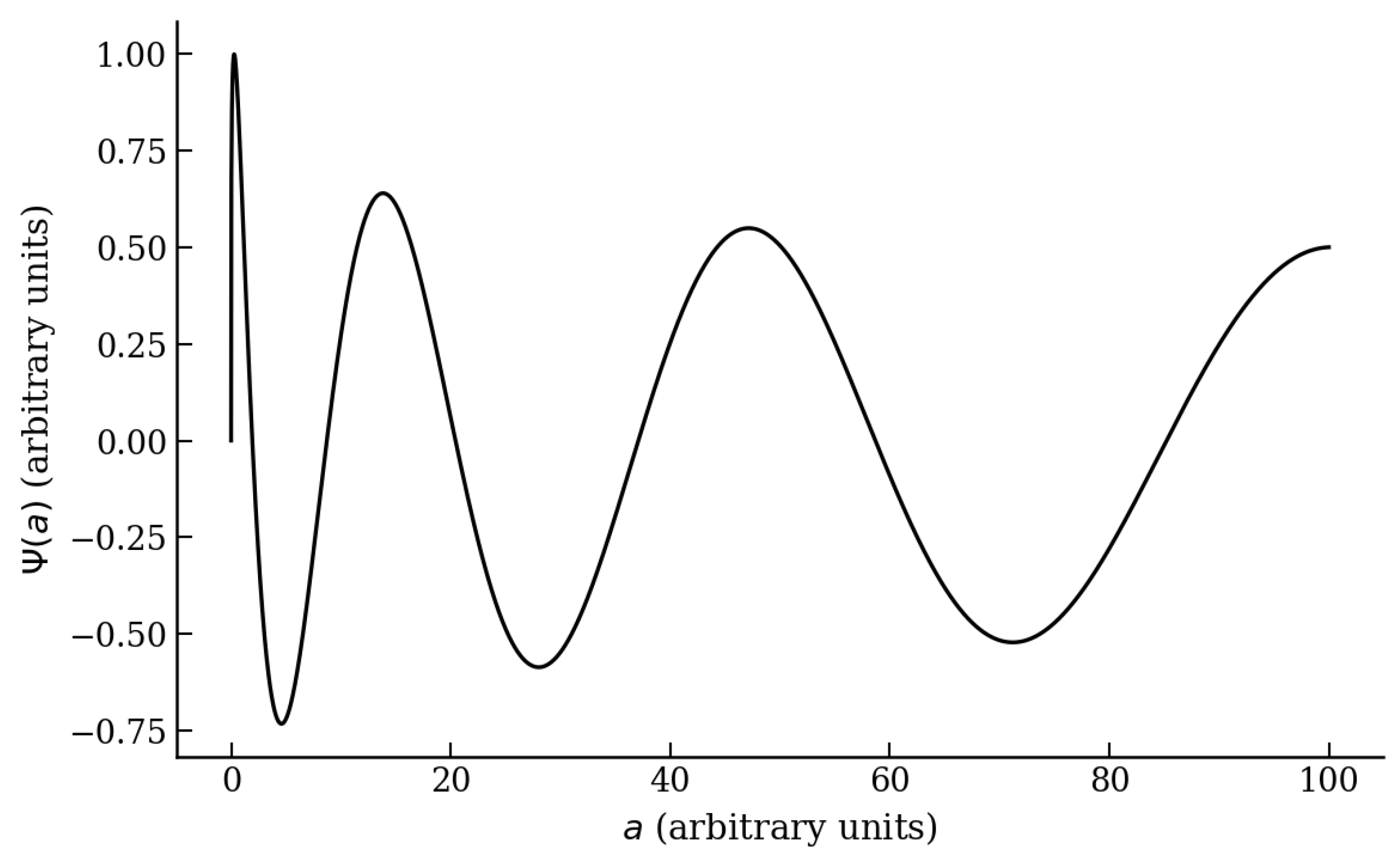
For large a,
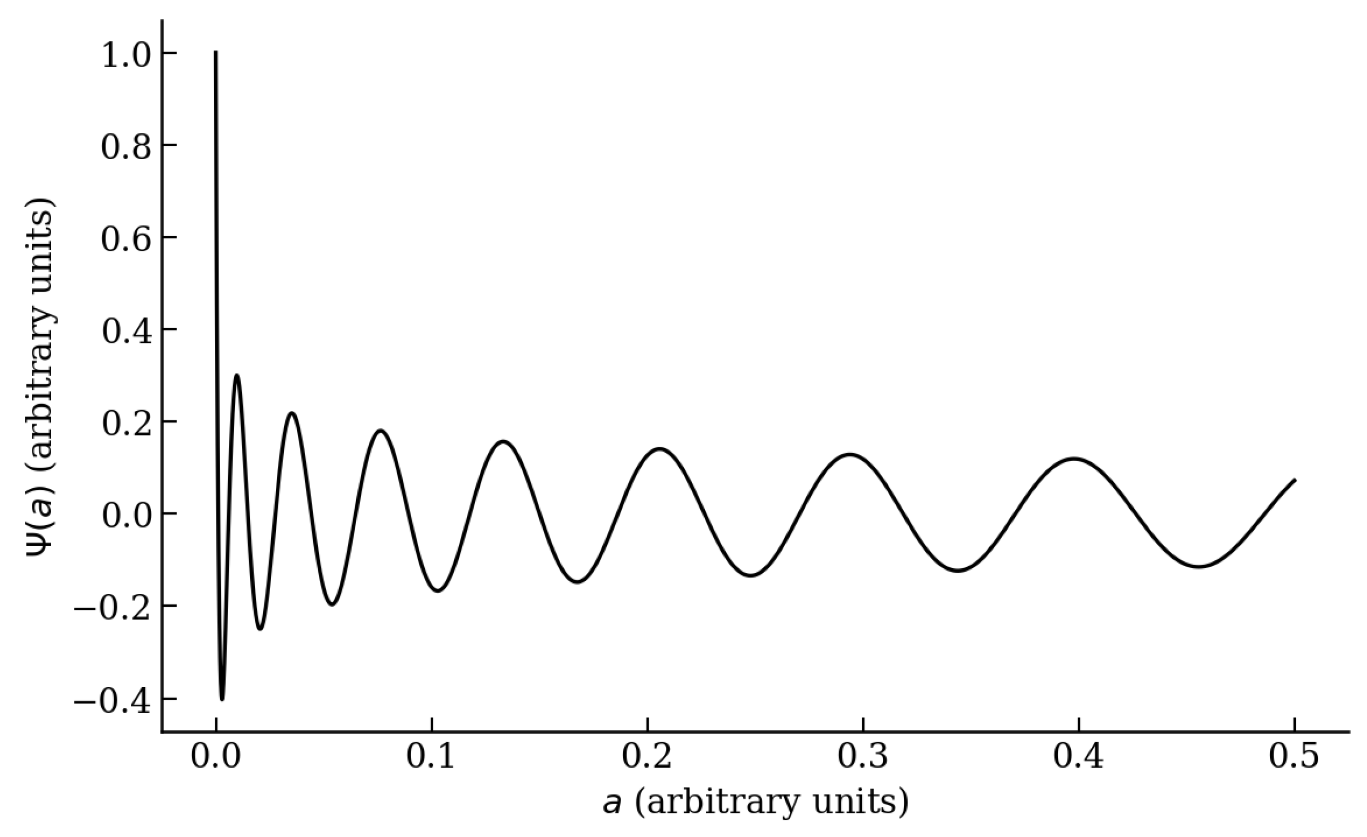
so the solution is again oscillatory with a slowly decaying envelope. The factor-ordering parameter therefore controls whether the origin is regular or suppressed.
Figure 3.
Dust-case Wheeler–DeWitt wave function for , , , , and . The regular solution remains finite and nonzero at . It therefore satisfies regularity at the origin, but not the DeWitt boundary condition.
Figure 3.
Dust-case Wheeler–DeWitt wave function for , , , , and . The regular solution remains finite and nonzero at . It therefore satisfies regularity at the origin, but not the DeWitt boundary condition.
3.4.3. A Non-Bessel Airy Example
The model also admits exact analytic sectors that are not of Bessel type. For
Equation (65) becomes
Defining
this becomes the standard Airy equation,
The general solution is
A DeWitt-compatible linear combination is obtained by imposing . Since
one obtains
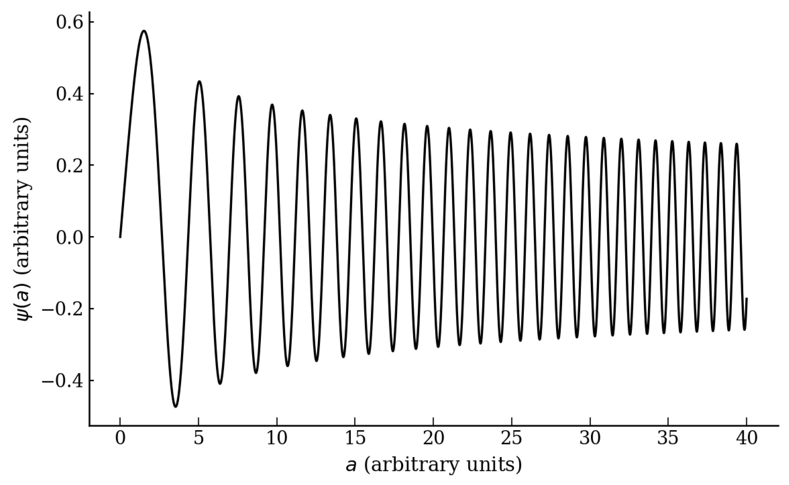
This solution vanishes at by construction and becomes oscillatory for large positive a. Although corresponds to an exotic equation of state rather than ordinary dust or radiation, the example is revealing because it shows that the scale-dependent model supports exact non-Bessel wave-function sectors.
Figure 4.
Airy-type Wheeler–DeWitt wave function for , , , , and . The linear combination is chosen so that , thereby satisfying the DeWitt condition.
Figure 4.
Airy-type Wheeler–DeWitt wave function for , , , , and . The linear combination is chosen so that , thereby satisfying the DeWitt condition.
3.4.4. Numerical Radiation-Era Example
As a radiation-era example, consider a radiation-dominated universe with
In this case Equation (64) has the schematic form
after collecting constants. The inverse-square term dominates as and produces a suppressed regular branch. At larger scale factor the positive linear term dominates, leading to an oscillatory regime. The numerical solution therefore transitions from suppression near to oscillatory behavior at larger a.
3.5. Local Airy form Near a Turning Point
Before turning to the full WKB analysis, we examine the local behavior near a simple turning point. Removing the first-derivative term by writing
the Wheeler–DeWitt equation takes the reduced form
Suppose that the effective potential has a simple turning point , so that
Expanding linearly,
Equation (89) reduces to Airy’s equation. The local solution may be written as
up to the sign convention associated with . Selecting the branch gives exponential suppression on the forbidden side of the turning point and oscillatory behavior on the allowed side. This is the standard local structure underlying WKB matching in quantum cosmology [4,5].
Figure 5.
Numerical Wheeler–DeWitt wave function for the radiation-dominated case , with , , , , and . The regular branch is suppressed near , satisfying the DeWitt condition, and becomes oscillatory at larger scale factor.
Figure 5.
Numerical Wheeler–DeWitt wave function for the radiation-dominated case , with , , , , and . The regular branch is suppressed near , satisfying the DeWitt condition, and becomes oscillatory at larger scale factor.
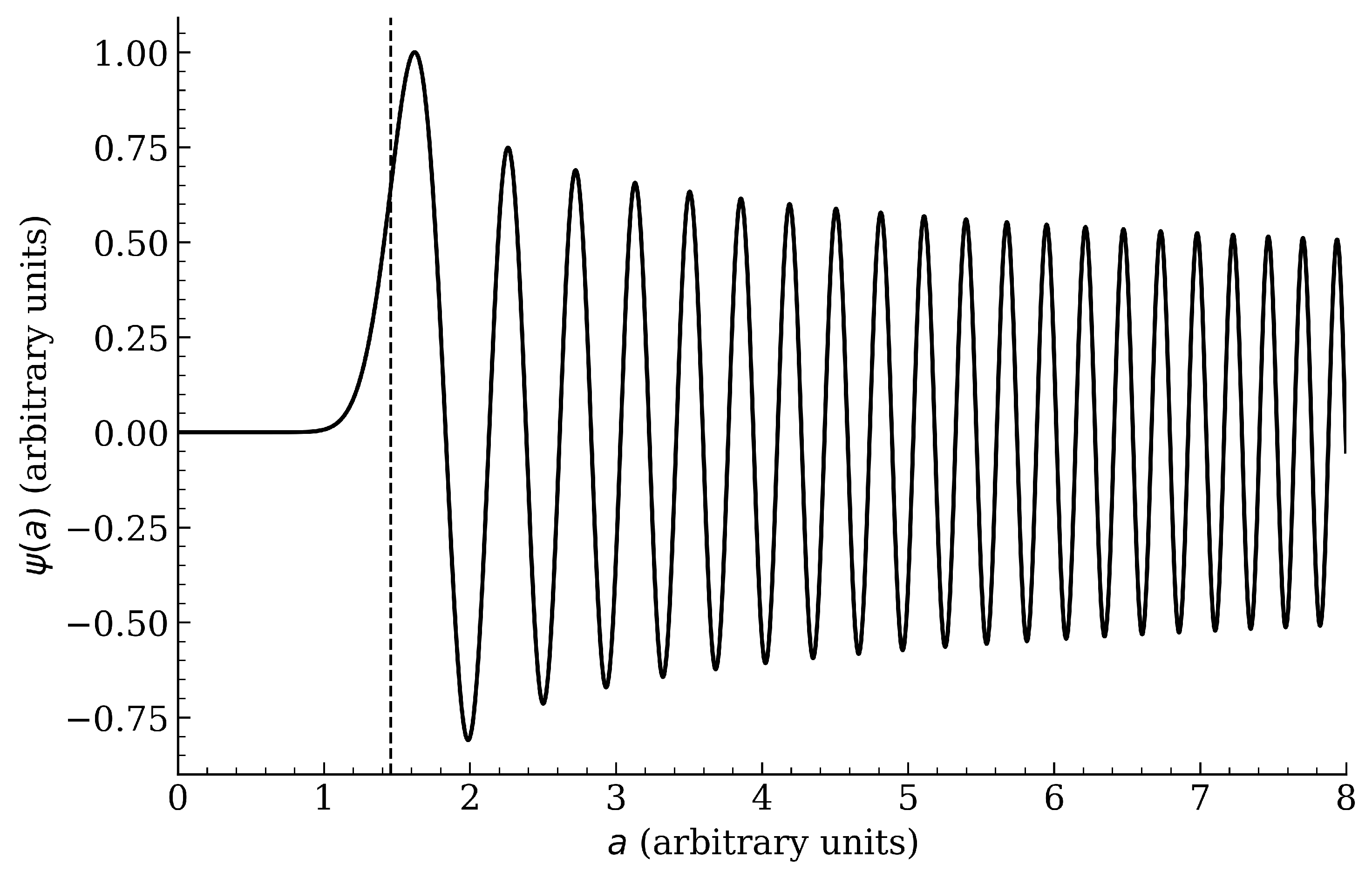
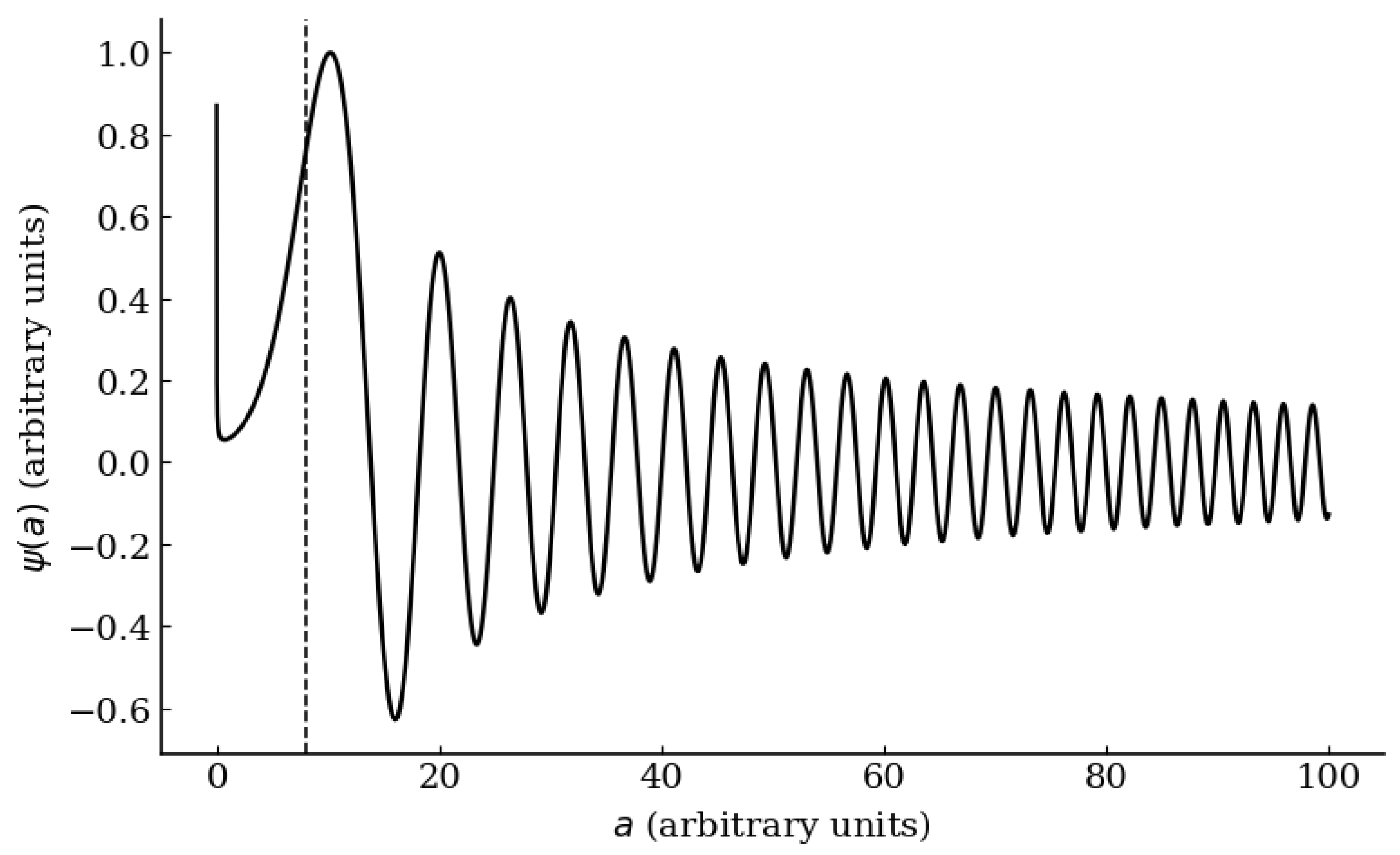
Figure 6.
Illustrative Airy-type semiclassical Wheeler–DeWitt wave function near a single turning point . The local form , shown here for , is exponentially suppressed on the forbidden side of the turning point and oscillatory on the allowed side. This figure illustrates the universal Airy matching behavior that appears near a simple Wheeler–DeWitt turning point.
Figure 6.
Illustrative Airy-type semiclassical Wheeler–DeWitt wave function near a single turning point . The local form , shown here for , is exponentially suppressed on the forbidden side of the turning point and oscillatory on the allowed side. This figure illustrates the universal Airy matching behavior that appears near a simple Wheeler–DeWitt turning point.
3.6. Summary of the Wheeler–DeWitt Sectors
The examples above show that the scale-dependent model admits several distinct quantum behaviors. The dust solution with is revealing: it is analytic, physically transparent, satisfies the DeWitt condition, and has a damped oscillatory large-a limit. The dust solution shows that regularity at is not the same as DeWitt suppression. The Airy example illustrates that the model is not restricted to Bessel-type sectors, while the radiation-era numerical solution provides a more familiar matter source in which the small-a region is suppressed and the large-a regime becomes oscillatory.
These results prepare us for the WKB analysis in Section 4. There, the same effective potential structure will be used to identify forbidden and allowed regions, turning points, and the branch interpretation of the minisuperspace wave function.
4. WKB Dynamics, Turning Points, and Probability Current
The exact solutions discussed in Section 3 show explicitly that the scale-dependent model admits wave functions that are either suppressed at the classical singularity or regular at the origin. We now turn to the WKB regime, where the connection between the Wheeler–DeWitt wave function and classical cosmological dynamics becomes explicit. The purpose of this section is to show how a forbidden small-a region, a turning point, and an oscillatory large-a branch arise in a representative case, and how the probability current distinguishes expanding and contracting semiclassical sectors.
We consider the flat dust-dominated model
with the quantum-correction parameter
This example is instructive because it reduces the Wheeler–DeWitt equation to a single-turning-point problem while retaining the effect of the running gravitational coupling. The resulting WKB structure is the familiar one: exponential behavior in a forbidden region, Airy matching near the turning point, and oscillatory behavior in the allowed region [4,5,29].
4.1. Reduced Wheeler–DeWitt Equation for a Chosen Model
We begin with the power-law Wheeler–DeWitt equation derived in Section 3,
For and , this becomes
For dust matter, , with and , the modified Friedmann function reduces to
Hence
For the representative value , this becomes
For ,
To remove the first-derivative term, we define
Equivalently,
4.2. Turning Point and WKB Regions
The turning point is determined by
For and , this gives the single positive turning point
The sign of then separates minisuperspace into two regions:
and
Thus the small-a region is WKB-forbidden, while the large-a region is WKB-allowed. This yields a forbidden small-a region and an allowed oscillatory large-a region.
For this choice of parameters,
one finds
This is the turning point shown in Figure 7.
4.3. Forbidden-Region and Allowed-Region Solutions
In the forbidden region , define
The WKB solution for is
where
Since , the corresponding WKB form for the original wave function is
The branch proportional to is suppressed as . Selecting this branch gives a wave function that is exponentially small in the classically forbidden small-a region.
In the allowed region , define
The WKB solution for is
where
Thus the original wave function is
4.4. Airy Matching Near the Turning Point
The connection between the forbidden and allowed WKB regions is obtained by matching to the local Airy solution near . Expanding about the turning point gives
where, using ,
Defining the local Airy scale
the reduced equation takes the standard Airy form near the turning point. The usual connection formula (see, e.g., [29,30]) gives the real matched solution in the allowed region as
The phase shift is the standard result for matching a decaying exponential on the forbidden side to an oscillatory solution on the allowed side.
This standing-wave form is the standard WKB continuation of a real decaying solution in the forbidden region. A purely outgoing or purely incoming branch may instead be selected by imposing an additional boundary condition in the allowed region.
4.5. Closed-Form WKB Actions and Asymptotic Behavior
For this case, the WKB actions can be evaluated analytically. In the forbidden region,
This expression vanishes at the turning point and diverges logarithmically as . Consequently, the decaying branch in Equation (116) is strongly suppressed near the classical singularity. In fact,
up to an overall constant.
In the allowed region,
For large a,
and the phase behaves as
Therefore the large-a wave function has the asymptotic form
The large-scale wave function is therefore oscillatory with a slowly decaying envelope. This is the usual WKB signature of a semiclassical regime.
The result is a WKB realization of the usual tunneling-type structure: a suppressed small-a region, a turning point, and an oscillatory large-a semiclassical branch. In the present model, this structure is generated by the scale dependence of the gravitational coupling and the associated -dependent correction.
4.6. Probability Current and Branch Interpretation
The WKB wave function becomes physically clearer when supplemented by the minisuperspace probability current. For the factor-ordered Wheeler–DeWitt equation
with real , the conserved current is
For the present model , this becomes
In the allowed region , the outgoing and incoming WKB branches are
Substitution into Equation (132) gives
up to the overall normalization of the wave function. Thus the outgoing branch carries positive flux, while the incoming branch carries negative flux. In this sense, the sign of the conserved current distinguishes expanding and contracting semiclassical branches [5].
By contrast, the real standing-wave combination
has
Similarly, a purely real decaying solution in the forbidden region carries no current. A nonzero conserved flux therefore appears only after selecting a complex traveling-wave branch in the WKB-allowed region. This is why the current is an invaluable diagnostic: oscillatory behavior alone does not specify a direction of semiclassical evolution, while the current does.
For the illustrative choice of values in Equation (112), one finds numerically that the current is constant across the allowed region:
This confirms the branch interpretation of the WKB solutions.
4.7. Hamilton–Jacobi Limit and Classical Recovery
The WKB phase also explains how the classical modified Friedmann dynamics are recovered. Starting from the compact Wheeler–DeWitt equation,
we use the WKB ansatz
At leading order in the WKB expansion, the phase satisfies
Identifying
and using the minisuperspace momentum
one immediately obtains
Thus the WKB Hamilton–Jacobi equation is exactly the classical modified Friedmann dynamics written in canonical form. The phase of the Wheeler–DeWitt wave function therefore encodes the classical cosmological trajectory [14,17].
The factor-ordering term affects the transport equation for the WKB amplitude, but not the leading Hamilton–Jacobi relation. The -dependent term should also be interpreted carefully: it originates from the quantum-corrected Friedmann equation before minisuperspace quantization. Thus the WKB expansion is an effective semiclassical expansion of an already quantum-corrected cosmological model, rather than a derivation of the term from the Wheeler–DeWitt quantization itself.
The physical picture is then consistent across the classical and quantum descriptions. The roots of determine the classical turning points. The same roots enter the Wheeler–DeWitt potential and determine where the WKB wave function changes from exponential to oscillatory behavior. In the oscillatory regime, the probability current separates expanding and contracting branches. In this way the WKB analysis connects the modified Friedmann dynamics, the minisuperspace wave function, and the emergence of semiclassical cosmological evolution.
5. Wheeler–DeWitt Equation with a Scalar-Field Clock
The Wheeler–DeWitt equation derived above is a constraint equation, so it does not contain an external time variable. To give the quantum theory a relational interpretation, we enlarge the minisuperspace from the single variable a to , where is a homogeneous free scalar field. Since the scalar field momentum is conserved, can be used as an internal clock on any classical branch for which [17,31].
We begin with the gravitational kinetic term used in the minisuperspace construction,
where the lapse function has been restored. For a homogeneous free scalar field, , the corresponding kinetic term is
The canonical momenta are therefore
Solving for the velocities and performing the Legendre transform gives the kinetic part of the Hamiltonian constraint,
The modified Friedmann equation can be written in the compact form
where denotes the full right-hand side of the scale-dependent Friedmann equation. The Hamiltonian constraint consistent with this classical limit is
Hence, if and , then , and Equation (149) reduces to , as required.
Upon quantization we take
and use the same factor ordering as above,
The Wheeler–DeWitt equation in the two-dimensional minisuperspace is then
Multiplying by , we obtain the more convenient form
This equation shows the structural change caused by the scalar clock: the scalar-field kinetic term enters with a coefficient proportional to . Thus the same running gravitational coupling that modifies also modifies the clock term itself.
For the power-law model
the scalar-clock contribution scales as
Hence the standard inverse-square clock term is recovered only when . For , the scalar-clock term becomes more singular as , while for it is softened.
We now separate variables by writing
where is the conserved scalar-field frequency. Since , Equation (153) becomes
For , this is
Using the normalized-density Friedmann function,
and the power-law effective couplings
with and , Equation (158) may be written as
where
The coefficient D carries the sign of k. Thus the curvature term should not be interpreted as positive-definite unless the curvature choice has already been fixed.
It is advantageous to remove the first-derivative term by defining
The mode equation becomes
with
This is the scalar-clock version of the Schrödinger-like Wheeler–DeWitt equation. Note that the new term’s scaling, , is controlled by the same exponent n as the gravitational term. The clock is therefore not an external add-on to the model; it is tied to the scale-dependent gravitational dynamics.
The relational interpretation can also be seen at the classical level. For a free scalar field,
and on a classical branch with and ,
Thus the roots of are also turning points of the relational evolution . This is why the same structure that produces a classical bounce or forbidden small-a region also appears in the scalar-clock Wheeler–DeWitt problem.
5.1. Wave Packets and Classical Recovery
The separated functions are mode functions. A semiclassical cosmological state should instead be built as a superposition of modes,
where is sharply peaked around . The Gaussian packet used below is not a new exact solution of the Wheeler–DeWitt equation, and it does not replace the Bessel, Airy, or WKB solutions discussed earlier. It is a narrow-packet approximation to a superposition of the Wheeler–DeWitt modes, used to describe how a localized state follows a classical trajectory in scalar-field time.
In the oscillatory regime, each mode may be written in WKB form as
The phase of the wave packet is then . Stationary phase gives
or
This relation defines the trajectory followed by the peak of the wave packet. In the semiclassical regime, that trajectory agrees with the classical relational solution determined by Equation (165).
The factor ordering also determines the natural minisuperspace measure on a constant- slice,
Therefore expectation values are defined by
In particular,
A state is semiclassical when
To see the classical limit explicitly, suppose the probability density is localized around the stationary-phase trajectory , with , and is well approximated near its peak by
Since the packet is assumed to be localized away from , the lower limit of the Gaussian integral may be extended to at leading order. With , expansion of the measure gives
Using the standard Gaussian moments, one obtains
and
Thus, to leading order,
For the Laplace–Beltrami ordering , this reduces to
The measure-induced shift of the packet center is therefore negligible whenever . Classical recovery fails near a turning point or near the small-a region, where the packet broadens and the quantum terms are no longer small.
5.2. Hamilton–Jacobi Limit and Probability Current
The same result follows from the Hamilton–Jacobi form of the Wheeler–DeWitt equation. Write
When is negligible, Equation (181) reduces to the classical Hamilton–Jacobi equation associated with Equation (149). This is the precise sense in which the modified Friedmann dynamics are recovered from the Wheeler–DeWitt phase in the large-scale, oscillatory regime.
The two-variable Wheeler–DeWitt equation also admits a conserved minisuperspace current. Multiplying Equation (153) by and using the fact that the coefficients are real gives
with
and
5.3. Interpretation of the Scalar-Clock Figure
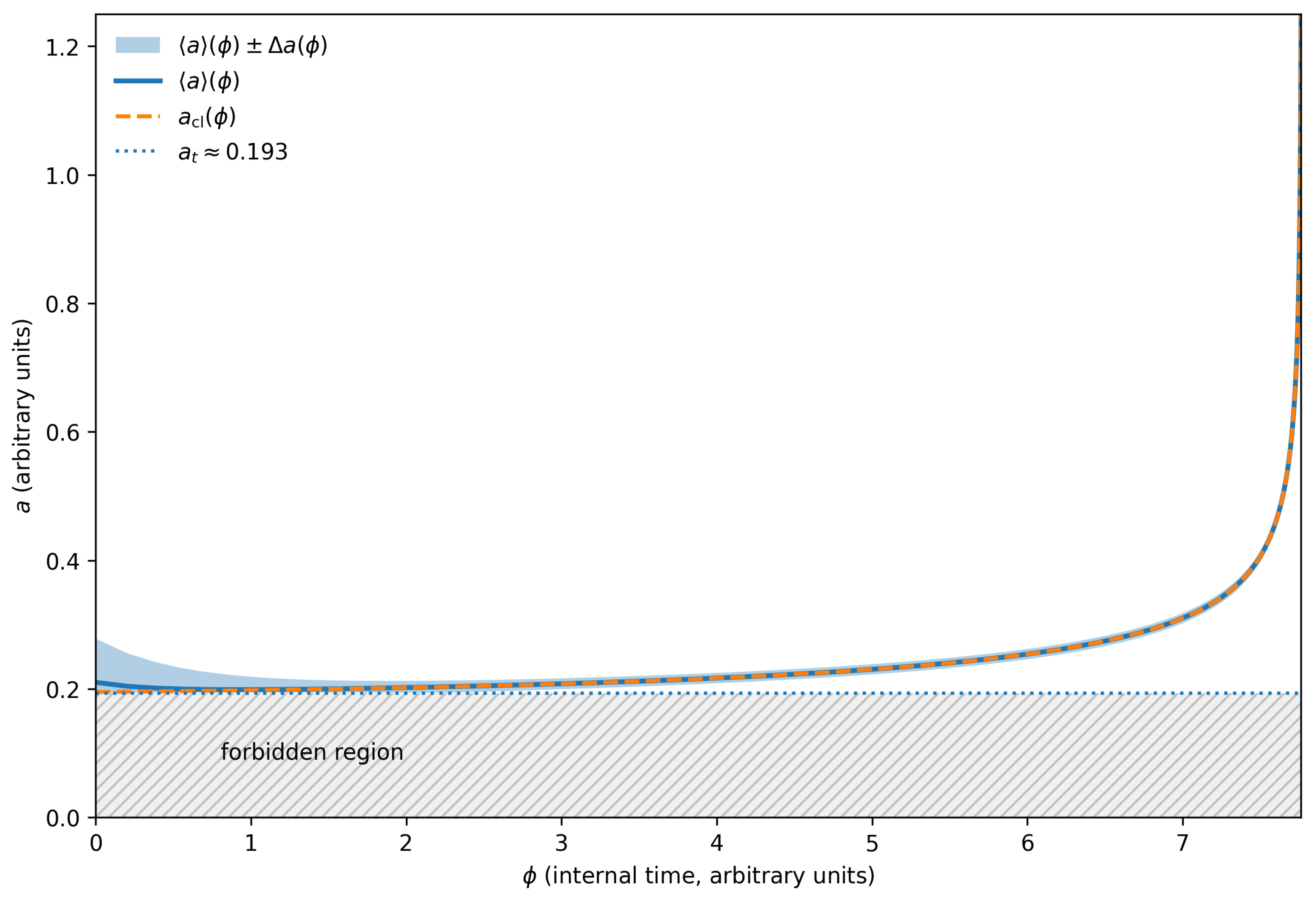
Figure 8 summarizes the scalar-clock interpretation. The dashed curve is the classical solution obtained from the same modified Friedmann function used in the Wheeler–DeWitt equation. The solid curve and shaded band show the expectation value and spread of a narrow quantum packet. Near the turning point, the packet is broad and the classical trajectory is not a good description of the state. At larger scale factor, the packet narrows relative to its mean value, and follows . This illustrates the quantum-to-classical transition.
The scalar field does not create a new Friedmann model; it gives the Wheeler–DeWitt wave function a relational time parameter. When contains a finite turning point, that same turning point appears in both the classical relational dynamics and the quantum mode structure. In the large-a oscillatory regime, the WKB phase, the conserved current, and the expectation value of a narrow packet all give the same semiclassical picture: the quantum state becomes peaked around the modified Friedmann trajectory. In the small-a region, the packet broadens and the quantum terms become critical, thus the classical description is no longer adequate.
6. Discussion
Allowing the gravitational coupling to depend on the scale factor modifies the first integral of the Newtonian equation of motion through the effective couplings , , and . Because these terms scale differently with a, the running reorganizes the small-scale structure of the modified Friedmann equation rather than simply rescaling Newton’s constant.
For the power-law ansatz , this reorganization is controlled entirely by the exponent n. In the dust, flat, case the matter and quantum-correction terms scale as and , respectively. These exponents coincide at , where the two terms lock onto the same power of a and no isolated turning point can exist. For the matter term is the more singular contribution near and carries a negative coefficient, so there, while the quantum-correction term restores at larger a. The root separating these regions is a genuine bounce. For the quantum term dominates but its coefficient is positive, so the small-a region remains classically allowed; any root in this window is a recollapse scale, not a bounce. The boundary marks the sign change of the quantum-correction coefficient.
A zero of is therefore not sufficient for singularity avoidance. A true bounce requires the additional sign condition: below the root and above it. Without this check, a formal turning point may be misidentified. Every root in the parameter survey of Sec. 2.8 is classified on this basis.
The Wheeler–DeWitt analysis is the quantum counterpart of the same statement. The running of enters the minisuperspace potential explicitly, and the resulting wave functions reflect the sign structure of the Friedmann equation. For the dust case with , the equation reduces to a Bessel problem. With the ordering , the regular solution satisfies the DeWitt condition ; with it is proportional to and remains finite but nonzero at the origin. DeWitt suppression and regular finite behavior at are physically distinct. The factor-ordering parameter controls which case applies, while the scale-dependent potential determines the structure of the Wheeler–DeWitt equation itself.
The Airy and radiation-era examples extend this picture beyond Bessel sectors. Their significance is not that they add new qualitative behavior but that they confirm the same three possibilities—DeWitt suppression, regularity, oscillatory large-a behavior—within different matter and running-exponent combinations, all from the same potential structure.
The WKB analysis sharpens the semiclassical reading. For the values of , , , , the reduced Wheeler–DeWitt equation has a single turning point at (in the arbitrary units of Eq. (112)). The WKB solution is exponentially suppressed for and oscillatory for . The conserved probability current then distinguishes the two oscillatory branches: the outgoing branch carries positive flux, the incoming branch negative flux, and a real standing-wave carries none. Oscillatory behavior alone does not select a direction of semiclassical evolution; the current does.
The scalar-field clock ties these threads together relationally. In the two-dimensional Wheeler–DeWitt equation (Eq. (153)), the clock term scales as , so the same exponent governing the running of also controls the small-a behavior of the relational dynamics.
The scope of this model is limited. It is an effective, homogeneous, isotropic minisuperspace model derived from a quantum-corrected Newtonian cosmology. This construction should therefore be interpreted as an effective minisuperspace quantization motivated by the modified Friedmann dynamics rather than as a derivation from the full Einstein–Hilbert action. It does not address anisotropies, inhomogeneous perturbations, or the full constraint algebra of general relativity. The coefficient is treated phenomenologically. The power law is a local early-time scaling ansatz; any complete model must account for the transition to the observed, effectively constant G at late times, as sketched in Sec. 2.7. The model instead provides a simplified minisuperspace framework in which the consequences of a running gravitational coupling can be tracked through the modified Friedmann equation to the Wheeler–DeWitt potential and semiclassical limit.
7. Conclusions
Starting from a quantum-corrected Newtonian cosmology with a scale-dependent gravitational coupling, we derived a modified Friedmann equation and corresponding Wheeler–DeWitt equation in which the running of changes the small-a structure of both the classical and quantum dynamics. For the power-law form , the dust, flat, model develops two natural analytic boundaries at and , separating regimes with qualitatively different turning-point and singularity structures.
Minisuperspace quantization leads to a Wheeler–DeWitt equation whose effective potential is determined by the same scale-dependent structure. Exact Bessel and Airy solutions, together with a numerical radiation-era example, exhibit three distinct behaviors near : DeWitt suppression (), regularity without suppression (), and oscillatory semiclassical behavior at large a. The factor-ordering parameter controls which of the first two applies; the model separates these cases, rather than conflating regularity with singularity avoidance.
The WKB analysis for the representative model (, , ) gives a forbidden small-a region, a single turning point, and an oscillatory large-a branch. The conserved probability current distinguishes expanding and contracting semiclassical branches, while the Hamilton–Jacobi limit recovers the modified Friedmann dynamics as the leading-order phase of the wave function. Introducing a homogeneous scalar field as an internal clock, wave packets can be constructed and followed in relational time: broad near the turning point, they narrow onto the classical trajectory at larger a. The clock term inherits the same running exponent n, coupling the timekeeping structure directly to the scale-dependent gravitational dynamics.
In the early-universe scaling regime considered here, the running of is not just a perturbative correction. This term changes the qualitative structure of both the classical and quantum cosmological equations, and the same scale dependence appears consistently across the Friedmann dynamics, Wheeler–DeWitt potential, WKB turning point, and scalar-clock semiclassical limit.
Several extensions are needed to determine whether this mechanism survives contact with observations. The full parameter space should be mapped systematically, with the Type I/II/III classification applied throughout, and the pure power law replaced by a transition profile such as Eq. (43) and matched to observational bounds. The phenomenological consequences of the running — its effect on the BBN expansion rate, the growth of linear matter perturbations, and the CMB acoustic scale — are examined in the companion paper [37], which shows that the strong running required for quantum singularity avoidance must cut off well before nucleosynthesis, and that the power-law model is best understood as an early-universe scaling limit rather than a global description of gravity.
Author Contributions
Conceptualization, J.A.S. and J.M.C.; methodology, J.A.S. and J.M.C.; software, R.B., B.R.F., and I.J.; validation, R.B., B.R.F., I.J., J.A.S. and J.M.C. ; formal analysis, R.B., B.R.F., and I.J.; investigation, J.A.S. and J.M.C; resources, J.A.S. and J.M.C.; writing—original draft preparation, J.A.S. and J.M.C.; writing—review and editing, J.A.S. and J.M.C.; visualization, R.B., B.R.F., I.J., J.A.S. and J.M.C. ; supervision, J.A.S. and J.M.C.; project administration, J.A.S. and J.M.C.; All authors have read and agreed to the published version of the manuscript.
Funding
This research received no external funding.
Institutional Review Board Statement
Not applicable.
Informed Consent Statement
Not applicable.
Data Availability Statement
No new data were created or analyzed in this study. Data sharing is not applicable to this article.
Conflicts of Interest
The authors declare no conflicts of interest.
Abbreviations and Symbols
The following abbreviations are used in this manuscript:
| WDW | Wheeler–DeWitt |
| WKB | Wentzel–Kramers–Brillouin |
| FRW | Friedmann–Robertson–Walker |
| LB | Laplace–Beltrami |
| QC | Quantum cosmology |
| SDG | Scale-dependent gravity |
| EOS | Equation of state |
The following symbols are used in this manuscript:
| a | Cosmological scale factor |
| R | Physical radius of the Newtonian sphere |
| Comoving reference radius | |
| H | Hubble parameter |
| Scale-dependent gravitational coupling | |
| Effective gravitational coupling appearing in the matter term | |
| Effective coupling associated with the classical correction term | |
| Effective coupling associated with the quantum correction term | |
| Energy density | |
| Present-day energy density | |
| Barotropic index in the equation of state | |
| k | Spatial curvature parameter |
| Effective coefficient of the higher-order classical correction | |
| Effective coefficient of the quantum correction term | |
| q | Factor-ordering parameter |
| Wheeler–DeWitt wave function | |
| Scalar-field internal clock | |
| Minisuperspace probability current |
References
- Penrose, R. Gravitational collapse and space-time singularities. Phys. Rev. Lett. 1965, 14, 57–59. [Google Scholar] [CrossRef]
- Hawking, S.W.; Ellis, G.F.R. The Large Scale Structure of Space-Time; Cambridge Monographs on Mathematical Physics; Cambridge University Press: Cambridge, UK, 1973. [Google Scholar]
- DeWitt, B.S. Quantum theory of gravity. I. The canonical theory. Phys. Rev. 1967, 160, 1113–1148. [Google Scholar] [CrossRef]
- Hartle, J.B.; Hawking, S.W. Wave function of the Universe. Phys. Rev. D 1983, 28, 2960–2975. [Google Scholar] [CrossRef]
- Vilenkin, A. Boundary conditions in quantum cosmology. Phys. Rev. D 1986, 33, 3560–3569. [Google Scholar] [CrossRef]
- Bojowald, M. Absence of a singularity in loop quantum cosmology. Phys. Rev. Lett. 2001, 86, 5227–5230. [Google Scholar] [CrossRef] [PubMed]
- Ashtekar, A.; Pawlowski, T.; Singh, P. Quantum nature of the Big Bang. Phys. Rev. Lett. 2006, 96, 141301. [Google Scholar] [CrossRef] [PubMed]
- Khoury, J.; Ovrut, B.A.; Steinhardt, P.J.; Turok, N. Ekpyrotic universe: Colliding branes and the origin of the hot Big Bang. Phys. Rev. D 2001, 64, 123522. [Google Scholar] [CrossRef]
- Gielen, S.; Magueijo, J. Quantum analysis of the recent cosmological bounce in the comoving Hubble length. Phys. Rev. D 2023, 107, 023518. [Google Scholar] [CrossRef]
- Gouba, L. Quantum Newtonian cosmology revisited. Lett. High Energy Phys. 2022, 5, 321. [Google Scholar]
- Leszczyńska, K. Quantum cosmology and varying physical constants. Universe 2017, 3, 46. [Google Scholar] [CrossRef]
- Donoghue, J.F. Leading quantum correction to the Newtonian potential. Phys. Rev. Lett. 1994, 72, 2996–2999. [Google Scholar] [CrossRef] [PubMed]
- Bargueño, P.; Bravo Medina, S.; Nowakowski, M.; Batic, D. Newtonian cosmology with a quantum bounce. Eur. Phys. J. C 2016, 76, 543. [Google Scholar] [CrossRef]
- Halliwell, J.J. Derivation of the Wheeler–DeWitt equation from a path integral for minisuperspace models. Phys. Rev. D 1988, 38, 2468–2481. [Google Scholar] [CrossRef]
- Senjaya, D. Exact solution to the Wheeler–DeWitt equation: Early and current Universe. J. High Energy Astrophys. 2024, 44, 494–499. [Google Scholar] [CrossRef]
- Bodmann, B.; Hadjimichef, D.; Hess, P.O.; de Freitas Pacheco, J.; Weber, F.; Razeira, M.; Degrazia, G.A.; Marzola, M.; Vasconcellos, C.A.Z. A Wheeler–DeWitt non-commutative quantum approach to the branch-cut gravity. Universe 2023, 9, 428. [Google Scholar] [CrossRef]
- Kiefer, C.; Peter, P. Time in quantum cosmology. Universe 2022, 8, 36. [Google Scholar] [CrossRef]
- Hamber, H.W.; Liu, S. On the quantum corrections to the Newtonian potential. Phys. Lett. B 1995, 357, 51–56. [Google Scholar] [CrossRef]
- Casadio, R.; Giugno, A.; Giusti, A.; Lenzi, M. Quantum corpuscular corrections to the Newtonian potential. Phys. Rev. D 2017, 96, 044010. [Google Scholar] [CrossRef]
- Scardigli, F.; Lambiase, G.; Vagenas, E.C. GUP parameter from quantum corrections to the Newtonian potential. Phys. Lett. B 2017, 767, 242–246. [Google Scholar] [CrossRef]
- Mandal, R.; Gangopadhyay, S.; Lahiri, A. Newtonian cosmology from quantum corrected Newtonian potential. Phys. Lett. B 2023, 839, 137807. [Google Scholar] [CrossRef]
- Hanımeli, E.T.; Tutusaus, I.; Lamine, B.; Blanchard, A. Low-redshift tests of Newtonian cosmologies with a time-varying gravitational constant. Mon. Not. R. Astron. Soc. 2020, 497, 4407–4415. [Google Scholar] [CrossRef]
- Barrow, J.D. Time-varying G. Mon. Not. R. Astron. Soc. 1996, 282, 1397–1406. [Google Scholar] [CrossRef]
- Reuter, M. Nonperturbative evolution equation for quantum gravity. Phys. Rev. D 1998, 57, 971–985. [Google Scholar] [CrossRef]
- Bonanno, A.; Saueressig, F. Asymptotically safe cosmology—A status report. Comptes Rendus Phys. 2017, 18, 254–264. [Google Scholar] [CrossRef]
- Faraoni, V. Cosmology in Scalar–Tensor Gravity; Kluwer Academic Publishers: The Netherlands, 2004. [Google Scholar]
- Overduin, J.M.; Wesson, P.S. Kaluza–Klein gravity. Phys. Rep. 1997, 283, 303–378. [Google Scholar] [CrossRef]
- Atkatz, D. Quantum cosmology for pedestrians. Am. J. Phys. 1994, 62, 619–627. [Google Scholar] [CrossRef]
- Bender, C.M.; Orszag, S.A. Advanced Mathematical Methods for Scientists and Engineers; McGraw-Hill: New York, NY, USA, 1978. [Google Scholar]
- Fröman, N.; Fröman, P.O. JWKB Approximation: Contributions to the Theory; North-Holland: Amsterdam, The Netherlands, 1965. [Google Scholar]
- Monerat, G.A.; Santos, C.G.M.; Alvarenga, F.G.; Gonçalves, S.V.B.; Fracalossi, R.; Corrêa Silva, E.V.; Oliveira-Neto, G. Quantum cosmology with many fluids and the choice of cosmological time. Braz. J. Phys. 2020, 50, 89–104. [Google Scholar]
- Kiefer, C. Quantum Gravity, 3rd ed.; Oxford University Press: Oxford, UK, 2012. [Google Scholar]
- Uzan, J.-P. Varying constants, gravitation and cosmology. Living Rev. Relativ. 2011, 14, 2. [Google Scholar] [CrossRef] [PubMed]
- Clifton, T.; Ferreira, P.G.; Padilla, A.; Skordis, C. Modified gravity and cosmology. Phys. Rep. 2012, 513, 1–189. [Google Scholar] [CrossRef]
- Pitrou, C.; Coc, A.; Uzan, J.-P.; Vangioni, E. Precision big bang nucleosynthesis with improved Helium-4 predictions. Phys. Rep. 2018, 754, 1–66. [Google Scholar] [CrossRef]
- Planck Collaboration. Planck 2018 results. VI. Cosmological parameters. Astron. Astrophys. 2020, 641, A6. [Google Scholar] [CrossRef]
- Furst, B.R.; Jarra, I.; Bolle, R.; Conroy, J.M.; Secrest, J.A. Scale-Dependent Gravity in Quantum Cosmology II: Phenomenological Consistency Tests from BBN, Structure Growth, and the CMB. in preparation, 2026.
Figure 1.
Bounce-scale survey for the power-law running model , shown for dust matter , flat spatial geometry , and vanishing classical correction , with . Panel (A) shows the true bounce scale as a function of the running exponent n for the reference value . The shaded region indicates parameter values for which no true bounce occurs, even though a formal turning point may exist. The vertical line at marks the degenerate case in which the relevant terms scale with the same power of a, and the marked point shows the representative value , for which . Panel (B) shows the sensitivity of the bounce scale to the quantum correction parameter for several values of n. This sensitivity becomes especially strong near , where the exponent in Equation (45) becomes large. Panel (C) gives the corresponding phase diagram in the plane, with contours of constant bounce scale. Panel (D) rewrites the bounce scale as a redshift, , allowing the bounce epoch to be compared with standard cosmological epochs. The result is that shifts the location of the bounce, while the existence of a true bounce is controlled primarily by the scaling exponent n. The redshift comparison in Panel (D) should be read as an illustrative normalization of the arbitrary unit bounce scale, not as a complete observational matching calculation.
Figure 1.
Bounce-scale survey for the power-law running model , shown for dust matter , flat spatial geometry , and vanishing classical correction , with . Panel (A) shows the true bounce scale as a function of the running exponent n for the reference value . The shaded region indicates parameter values for which no true bounce occurs, even though a formal turning point may exist. The vertical line at marks the degenerate case in which the relevant terms scale with the same power of a, and the marked point shows the representative value , for which . Panel (B) shows the sensitivity of the bounce scale to the quantum correction parameter for several values of n. This sensitivity becomes especially strong near , where the exponent in Equation (45) becomes large. Panel (C) gives the corresponding phase diagram in the plane, with contours of constant bounce scale. Panel (D) rewrites the bounce scale as a redshift, , allowing the bounce epoch to be compared with standard cosmological epochs. The result is that shifts the location of the bounce, while the existence of a true bounce is controlled primarily by the scaling exponent n. The redshift comparison in Panel (D) should be read as an illustrative normalization of the arbitrary unit bounce scale, not as a complete observational matching calculation.
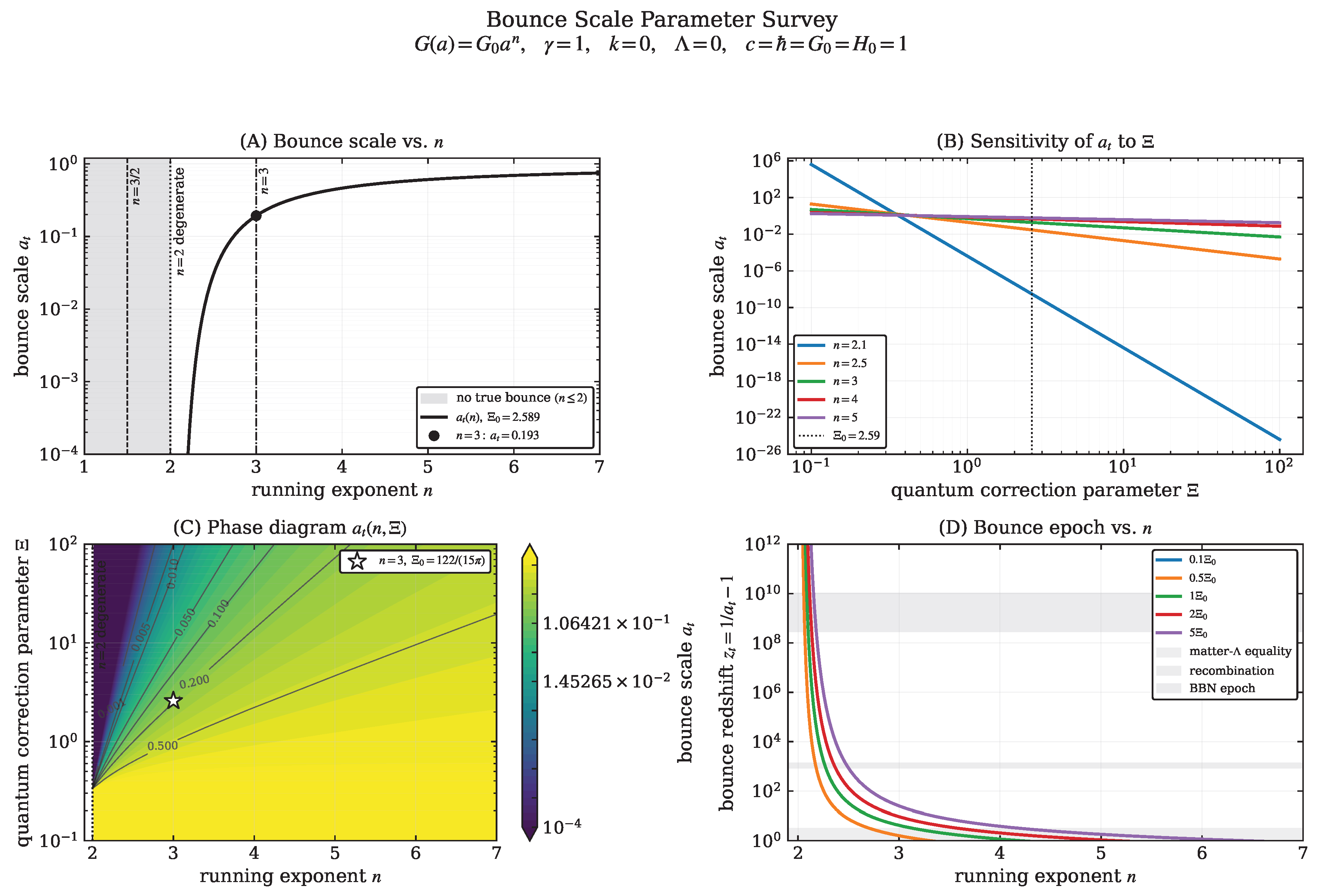
Figure 7.
WKB wave function for the example case , , , , , and , shown in arbitrary units. The dashed vertical line marks the turning point , which separates the small-a WKB-forbidden region from the large-a WKB-allowed region. For , the wave function is exponentially suppressed, while for it becomes oscillatory with a slowly decaying envelope.
Figure 7.
WKB wave function for the example case , , , , , and , shown in arbitrary units. The dashed vertical line marks the turning point , which separates the small-a WKB-forbidden region from the large-a WKB-allowed region. For , the wave function is exponentially suppressed, while for it becomes oscillatory with a slowly decaying envelope.
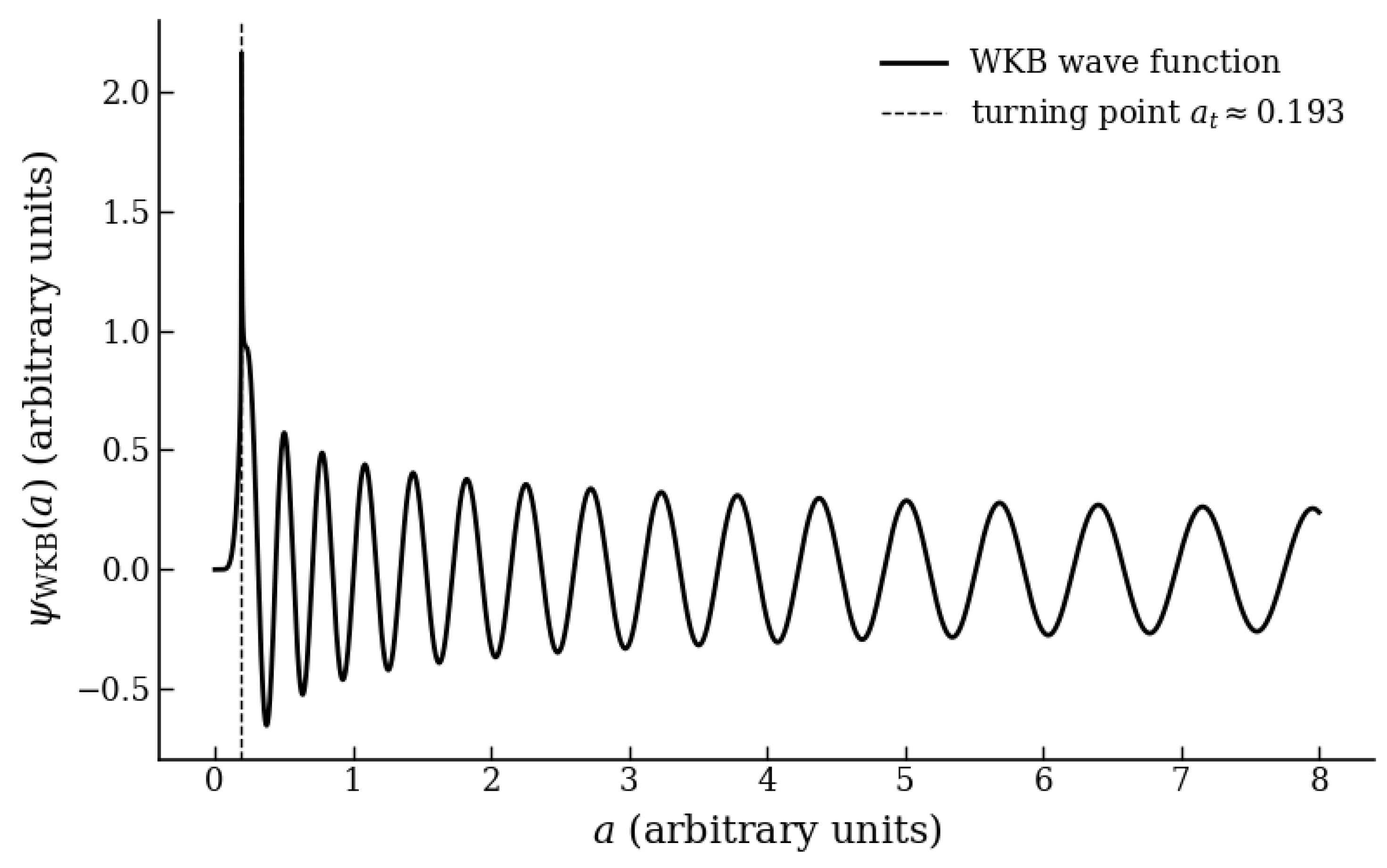
Figure 8.
Quantum-to-classical correspondence in scalar-field time for the case , , , , , and , shown in arbitrary units. The dashed curve shows the classical relational trajectory obtained from Equation (165). The solid curve shows the expectation value , and the shaded band represents the quantum spread . The horizontal dotted line marks the turning point , defined by , while the hatched region denotes the classically forbidden sector. The figure illustrates that the state is broad near the turning point but becomes sharply peaked around the classical trajectory at larger scale factor.
Figure 8.
Quantum-to-classical correspondence in scalar-field time for the case , , , , , and , shown in arbitrary units. The dashed curve shows the classical relational trajectory obtained from Equation (165). The solid curve shows the expectation value , and the shaded band represents the quantum spread . The horizontal dotted line marks the turning point , defined by , while the hatched region denotes the classically forbidden sector. The figure illustrates that the state is broad near the turning point but becomes sharply peaked around the classical trajectory at larger scale factor.
Disclaimer/Publisher’s Note: The statements, opinions and data contained in all publications are solely those of the individual author(s) and contributor(s) and not of MDPI and/or the editor(s). MDPI and/or the editor(s) disclaim responsibility for any injury to people or property resulting from any ideas, methods, instructions or products referred to in the content. |
© 2026 by the authors. Licensee MDPI, Basel, Switzerland. This article is an open access article distributed under the terms and conditions of the Creative Commons Attribution (CC BY) license (http://creativecommons.org/licenses/by/4.0/).
Copyright: This open access article is published under a Creative Commons CC BY 4.0 license, which permit the free download, distribution, and reuse, provided that the author and preprint are cited in any reuse.


