Boundary Terms, Finite FLRW Spacetimes, and the Emergence of the Cosmological Constant Λ

1. Introduction

The origin of the cosmological constant $\Lambda$ remains one of the deepest open problems in gravitation and cosmology. Observations indicate that the present Universe is undergoing accelerated expansion consistent with a small but non-zero effective cosmological constant, corresponding to an energy density of order ${\rho }_{\Lambda }\sim {10}^{-29}\mathrm{g}{\mathrm{cm}}^{-3}$. Within the standard cosmological model, this is usually described by Einstein’s field equations with a cosmological constant $\Lambda$:

$$G_{\mu \nu }+\Lambda g_{\mu \nu }=8\pi G{T}_{\mu \nu }.$$

(1)

Although this phenomenological description agrees remarkably well with observations, the physical origin of $\Lambda$ remains unclear. Estimates of vacuum energy from quantum field theory exceed the observed value by many orders of magnitude, giving rise to the well-known cosmological constant problem [1,2]. From the perspective of General Relativity, the cosmological constant enters naturally through the Einstein-Hilbert (EH) action:

$$S_{\mathrm{EH}}={\displaystyle \frac{1}{16\pi G}}{\int }_{\mathcal{M}}{d}^{4}x\sqrt{-g}(R-2\Lambda ),$$

(2)

where $\Lambda$ can be viewed either as a fundamental constant of the action or as an effective contribution arising from vacuum energy, modified gravity, or other microscopic physics.

An often underemphasized aspect of the EH action is that its variational principle depends crucially on boundary terms and on the boundary data held fixed during the variation [3]. In standard textbook derivations, varying the EH action generates a boundary contribution involving variations of the boundary metric and its normal derivatives. To obtain a well-defined variational principle under Dirichlet boundary condition, one usually fixes the induced metric: $\delta h_{ab}=0$, where $h_{ab}$ is the metric induced on the boundary hypersurface. Under such conditions, one could artificially add the Gibbons–Hawking–York (GHY) boundary term to cancel the remaining surface variation [4,5,6,7]. However, the key issue is not whether one adds the GHY term or not. The more fundamental question is: what boundary data are physically fixed?

This distinction becomes crucial when the boundary is not a fixed outer hypersurface but a junction hypersurface $\Sigma$ connecting two spacetime regions. In such problems, one is not imposing ordinary Dirichlet conditions at a finite boundary or at spatial infinity. Instead, one requires that the total action of the joined spacetime remains stationary:

$$\delta S_{\Sigma }=0.$$

(3)

This is a stronger and more specific requirement than the standard fixed-boundary variational problem. In this setting, the natural condition is not simply $\delta h_{ab}=0$, but rather the continuity conditions associated with the junction, involving both the induced metric and the extrinsic curvature. Junction problems therefore belong to a fundamentally different class from the standard Dirichlet boundary problem.

In this work, we study such a junction problem for a finite Friedmann–Lemaître–Robertson–Walker (FLRW) spacetime matched to an exterior vacuum. This setup defines a finite gravitating FLRW region whose boundary is determined dynamically by the global variational principle rather than something that is imposed by hand.

The Openheimer–Snyder solution with pressureless matter [8] remains one of the few exact analytical models of gravitational collapse in General Relativity. Its simplicity relies crucially on the absence of pressure, which ensures that the collapsing matter follows geodesic motion and allows a comoving FLRW interior to be matched exactly to an exterior Schwarzschild spacetime. Once pressure is introduced, the fluid no longer follows geodesics, the matching problem becomes considerably more difficult, and exact analytical FLRW interior solutions are generally believed to be unavailable [9,10,11].

One of the main results of the present work is to show that this conclusion is too restrictive. We show here that the boundary equation admits two physically distinct branches. The first is a trivial comoving branch with vanishing peculiar velocity, $v=0$, which reproduces the standard Oppenheimer–Snyder dust solution and requires the cosmological constant to vanish on both sides of the boundary. This branch is therefore of limited relevance for cosmology, since the observed Universe contains $\Lambda$, radiation, and pressure components. The physically relevant solution is a non-comoving branch satisfying $v>0$, which exists whenever pressure or $\Lambda$ components are present. This branch evolves toward a universal null attractor $v\to 1$ independent of spatial curvature when v is properly defined.

A related approach to the cosmological constant as a boundary condition has been explored in earlier work [12,13,14]. These previous analyses also relied on limiting cases of the junction dynamics and on partial use of the full variational principle. In the present work, we extend the result for the case with curvature and clarify how the finite-Universe realisation emerges as an exact consequence of the variational principle. The more general case will be presented elsewhere.

A different interpretation of the cosmological constant as a boundary condition was previously proposed in [15,16], where $\Lambda$ was related to a zero-action condition imposed on a finite causal domain. In that earlier approach, the asymptotic recovery of empty space was effectively implemented by requiring the FLRW interior to satisfy an asymptotic condition equivalent to $\ddot{a}\to 0$, leading to the relation $\Lambda \simeq 4\pi G\langle \rho +3p\rangle$. The present work clarifies and improves that interpretation in several important ways. First, we show that asymptotic flatness need not be enforced through the asymptotic behaviour of the FLRW interior itself. Instead, the FLRW region may remain finite and be matched consistently to an exterior Schwarzschild (or more generally Schwarzschild–deSitter/Anti-deSitter) spacetime. Empty Minkowski space is then recovered in the exterior region, not as a limit of the interior FLRW solution. Second, the cosmological constant is derived here from the exact variational principle and junction conditions, without invoking volume averages or heuristic zero-action arguments. Thus, the earlier boundary interpretation is not discarded but generalised: the present formulation provides a mathematically precise realisation of the same underlying idea, while removing assumptions that were specific to the earlier approximate treatment.

This investigation further advances in fixing the physical understanding of the arbitrary cosmological constant that can always be added to the EH action. The variational boundary value problem in our framework brings this cosmological constant to a specific value associated with the inverse square of the Schwarzschild radius ($r_s=2GM$) below which a finite FLRW Universe evolves with a non-comoving boundary. The larger the asymptotic boundary (i.e., $r_s$) of the finite Universe, the smaller the value of the cosmological constant ($\Lambda ={\displaystyle \frac{3}{r_s^2}}$) a comoving FLRW observer witnesses. We show that the non-comoving boundary of the finite FLRW cloud leads to the understanding of current de Sitter-like accelerated expansion. Thus, we not only explain the smallness of the cosmological constant but also unify the Schwarzschild horizon of the superior observer with the de Sitter horizon of the comoving observer of the FLRW Universe. We also address other conceptual issues associated with the cosmological constant problem under the boundary condition of the variational principle. This brings a new revelation that we can add any number of cosmological constants (such as a combination of standard arbitrary cosmological constant, vacuum energy from matter fields of the standard (particle physics) model, or beyond, or even a negative cosmological constant) to the EH action, and the boundary condition fixes the sum to be inversely proportional to the Schwarzschild radius square. This significantly revises our understanding of the cosmological constant.

Throughout the paper we follow the metric signature $\left(-+++\right)$. We follow Greek indexes $(\mu ,\nu )$ and $x_{\mu }$ coordinates operate within 4D manifold $\mathcal{M}$, while Latin indexes $(a,b)$ and $y_a$ coordinates operate within the 3D hypersurface $\Sigma$ or submanifold $\partial \mathcal{M}$.

2. Einstein–Hilbert Action and the Variational Principle

The fundamental laws of physics are often obtained by requiring an action functional to be stationary under infinitesimal variations of the dynamical fields. For gravity, the configuration is the geometry itself — the metric $g_{\mu \nu }$. The Einstein–Hilbert action encodes the curvature of spacetime governed by the matter and energy content.

Given $\mathcal{M}$, the four-dimensional manifold or bulk, the Einstein–Hilbert action minimally coupled to reads:

$$S_{\mathrm{EH}}\left[\mathcal{M}\right]={\int }_{\mathcal{M}}d\mathcal{M}\left[{\displaystyle \frac{R}{16\pi G}}+{\mathcal{L}}_m\right],$$

(4)

where ${\mathcal{L}}_m$ is the matter Lagrangian and $d\mathcal{M}=\sqrt{-g}{d}^{4}x$ is the invariant volume element. Applying the variational principle to the EH action Eq.4 $\delta S_{\mathrm{EH}}=0$, gives

$$\begin{array}{ccc}\hfill G_{\mu \nu }& \equiv & R_{\mu \nu }-{\displaystyle \frac{1}{2}}{g}_{\mu \nu }R\hfill \\ \hfill & =& 8\pi G{T}_{\mu \nu }\equiv -{\displaystyle \frac{16\pi G}{\sqrt{-g}}}{\displaystyle \frac{\delta \left(\sqrt{-g}{\mathcal{L}}_m\right)}{\delta g^{\mu \nu }}},\hfill \end{array}$$

(5)

which are the well-known Einstein’s field equations. But the standard derivation of Eq.5 ignores or implicitly assumes the boundary variations of the metric to be zero by hand, which we will show shortly in detail.

The variational principle highlights something often overlooked: even though the field equations are local relations, the action itself is global. It integrates curvature and matter over the entire spacetime region under consideration. This global perspective becomes essential when comparing different possible histories of the Universe or when extending gravity into the quantum domain.

3. Boundary Terms

One subtlety arises immediately when varying the Einstein–Hilbert action: total derivatives appear and generate boundary terms. If these terms are ignored, the variational principle becomes incomplete, and the derivation of Einstein’s equations is not mathematically well posed. In some situations the boundary contributions vanish automatically, for example, when fields fall off sufficiently rapidly at infinity. However, this is no longer true when spacetime has nontrivial boundaries or horizons.

This point is the central theme of this work: gravity is not only about local curvature, but also about global structure. Boundaries, whether located at infinity, at black-hole horizons, or at the edge of a finite cosmological region, play a key role in understanding the spacetime geometry. These terms influence the global properties of spacetime and, in cosmology, may even contribute to the effective value of the cosmological constant itself.

All of this understanding emerges from the variation of the Einstein–Hilbert action Eq.4, which contains a "total derivative" term [3]:

$$\delta S_{\mathrm{EH}}={\int }_{\mathcal{M}}{\displaystyle \frac{d\mathcal{M}}{16\pi G}}\left[\left(G_{\mu \nu }-8\pi G{T}_{\mu \nu }\right)\delta g^{\mu \nu }+{\nabla }_{\rho }{V}^{\rho }\right].$$

where $V^{\rho }\equiv g^{\mu \nu }\delta {\Gamma }^{\rho }{}_{\mu \nu }-g^{\rho \sigma }\delta {\Gamma }_{\mu \sigma }^{\mu }$. Using the divergence theorem, this term becomes a surface contribution:

$$\delta S_{\partial \mathcal{M}}={\int }_{\mathcal{M}}d\mathcal{M}{\nabla }_{\mu }{V}^{\mu }={\int }_{\partial \mathcal{M}}{d}^{3}y\sqrt{\left|h\right|}{n}_{\mu }{V}^{\mu }.$$

(6)

Here $\partial \mathcal{M}$ denotes the spacetime boundary, represented by a non-null hypersurface $\Sigma$ with unit normal $n_{\mu }$, and $h_{ab}=h_{ab}\left(y\right)$ is the corresponding induced metric: i.e. $g_{\mu \nu }\equiv g_{\mu \nu }\left(x\right)$ on the boundary. For the timelike boundary ($\left|h\right|=-h$), the normal vector is $n_{\mu }{n}^{\mu }=1$ spacelike, whereas the spacelike boundary ($\left|h\right|=h$) has a timelike normal vector $n_{\mu }{n}^{\mu }=-1$. The tangent basis vectors to $\Sigma$ are defined by

$$e^{\mu }{}_a:={\displaystyle \frac{\partial x^{\mu }}{\partial y^a}},n_{\mu }{e}^{\mu }{}_a=0,$$

(7)

which gives the induced metric $h_{ab}=g_{\mu \nu }{e}^{\mu }{{}_{a}e^{\nu }}_b$. The surface variation can be separated into two contributions (see [3]):

$$\delta S_{\partial \mathcal{M}}=\delta S_K+\delta S_h,$$

(8)

where

$$\begin{array}{cc}\hfill \delta S_K& ={\int }_{\partial \mathcal{M}}{d}^{3}y\delta \left(2\sqrt{\left|h\right|}K\right)\hfill \\ \hfill \delta S_h& ={\int }_{\partial \mathcal{M}}{d}^{3}y\sqrt{\left|h\right|}(K{h}_{ab}-K_{ab})\delta h^{ab}\hfill \\ \hfill K_{ab}& =-e_a^{\mu }{e}_b^{\nu }{\nabla }_{\mu }{n}_{\nu },K=h^{ab}{K}_{ab},\hfill \end{array}$$

(9)

The extrinsic curvature tensor of the boundary hypersurface, is given by the covariant derivative ${\nabla }_{\mu }$ of the normal $n_{\mu }$. Since $K_{ab}$ contains the normal derivative of the induced metric, fixing $K_{ab}$ is the gravitational analogue of imposing Neumann boundary conditions, the remaining condition is then $\delta S_h=0$. The term $\delta S_K$ corresponds to the Gibbons–Hawking–York (GHY) boundary term (see [6,17]). It is required when imposing Dirichlet boundary conditions, for which the induced metric is fixed: $\delta h_{ab}=0$ so that $\delta S_h=0$. The role of the GHY term is to cancel the variations involving normal derivatives of the metric (equivalently, variations of the extrinsic curvature), so that the variational principle becomes well defined when the induced metric $h_{ab}$ is held fixed at the boundary. By contrast, Neumann-type boundary conditions correspond to fixing the extrinsic curvature itself rather than the induced metric. In that case the term $\delta S_h=0$ becasue K is fixed.

A well-defined variational principle requires the total boundary, $\partial \mathcal{M}$, variation $\delta$ of the action S to vanish:

$$\delta S_{\partial \mathcal{M}}=0.$$

(10)

The choice of boundary conditions is therefore not merely a mathematical detail. Different physical boundaries impose different geometric constraints on spacetime. In gravitational systems with horizons or finite domains, these consistency conditions can introduce additional global relations between geometry and matter. This is in addition to the regular Einstein field equations.

3.1. Boundary and Junction Conditions

Consider a spacetime formed by the union of two manifolds:

$$\mathcal{M}={\mathcal{M}}^{-}\cup \Sigma \cup {\mathcal{M}}^{+},$$

(11)

where the interior region is ${\mathcal{M}}^{-}$ and the exterior region ${\mathcal{M}}^{+}$, with $\Sigma$ is the junction hypersurface between the two.

What role do the boundary terms discussed previously play in this construction? If we choose ${\mathcal{M}}^{+}$ to be empty space (or a manifold without any other boundaries), the matching hypersurface $\Sigma =\partial \mathcal{M}$ acts as the physical boundary of the ${\mathcal{M}}^{-}$ manifold. A sufficient condition for the total variational principle $\delta S=0$ requires Einstein’s equations inside each region and also consistency of the total boundary/junction variation:

$$G_{\mu \nu }^{(\pm )}=8\pi G{T}_{\mu \nu }^{(\pm )}\mathrm{in}{\mathcal{M}}^{\pm },\delta S_{\Sigma }=0.$$

(12)

This requires: $S_{\Sigma }=\delta S_{\partial \mathcal{M}}=\delta S_K+\delta S_h=0$ in Eq.8. Because the normal to $\Sigma$ has opposite signs in both sides of $\Sigma$, the continuity of the induced metric $h_{ab}$ and its normal derivative $K_{ab}$ implies $\delta S_{\partial \mathcal{M}}=0$ in Eq.8. So in the absence of a surface stress-energy layer, this is equivalent to the the Darmois [18] (Israel [19,20] with no shell) junction conditions. In this sense, $\delta S_{\Sigma }=0$ plays a dual role: it is simultaneously the geometric matching condition between the two manifolds and the condition required for a globally consistent variational principle. No additional boundary terms, such as the GHY term, are needed.

This is not necessarily the most general solution, but is a sufficient condition to provide an exact solution to GR. More generally, one could have solutions where $\delta S_{\Sigma }$ compensates $\delta S_{{\mathcal{M}}^{\pm }}$ so that the total variation remains $\delta S=0$.

3.2. Background Exterior Spacetime

We will assume that the FLRW metric correspond to a perturbation in a larger background, so that the external background correspond to a spherically symmetric perturbation:

$$d{s}^2=-(1+2\Psi )d{t}^2+{\displaystyle \frac{d{r}^2}{1+2\Phi }}+r^{2}d{\Omega }^2$$

(13)

We will focus here in the case of static Newtonial potentials $\Phi =\Psi =\Psi \left(r\right)$ but we will present the non symmetric elsewhere. For a perfect fluid this results in constant energy density $\rho$, which corresponds to Schwarzschild ($\rho =0$), de-Sitter ($\rho ={\rho }_{\Lambda }^{+}$) or combination:

$$\begin{array}{ccc}\hfill d{s}^2& =& -F\left(r\right)d{t}^2+{\displaystyle \frac{d{r}^2}{F\left(r\right)}}+r^{2}d{\Omega }^2,\hfill \\ \hfill F\left(r\right)& \equiv & 1+2\Phi =1-{\displaystyle \frac{r_s}{r}}-{\displaystyle \frac{{\Lambda }^{+}}{3}}{r}^2\hfill \end{array}$$

(14)

This is the Schwartzschild vacuum solution with a $\Lambda$ term, which we label ${\Lambda }^{+}=8\pi G{\rho }_{\Lambda }^{+}$, a free parameter in the local equations. This results in a deSitter (Minkowski) phase at large radius r for ${\Lambda }^{+}\ne 0$ (${\Lambda }^{+}=0$).

3.3. Empty Space

Consider two generic spherically symmetric metrics in rest frame coordinates $(t,r)$ in Eq.13. This can represent both a FLRW metric or some empty space. We consider a solution which is the combination of two metrics with a junction $R=r\left(t\right)$. We have shown that for this to be a solution to the Einstein-Hilbert action the sufficient condition (that avoids boundary terms) is that the junction complies with the Darmois [18] (Israel with no shell) junction conditions.

We will label ${\Phi }_{+}$ and ${\Psi }_{+}$ the exterior metric and ${\Phi }_{-}$ and ${\Psi }_{-}$ the interior one. Our goal is to have FLRW interior with ${\rho }_{-}\ne 0$ and empty exterior with ${\rho }_{+}=0$. This is what we call a Black Hole Universe.

For a FLRW without $\Lambda$ and negligible pressure (dust universe) the solution is to have a comoving junction $\dot{R}=HR$ join to a Schwarzschild metric. This provides an exact solution to the Einstein-Hilber action.

For the FLRW metric with $\Lambda$ we note that it asymptotically evolves into deSitter metric (${\Psi }_{-}={\Phi }_{-}=r^2/R_{\Lambda }^2$) which has a causal horizon at the null surface $r=R_{\Lambda }=\sqrt{3/\Lambda }$. The FLRW metric inside $r<R_{\Lambda }$ is causally isolated from $r>R_{\Lambda }$. For this reason we expect that we can match it with an empty exterior.

In deSitter limit we have shown that the junction $R\left(\tau \right)$ with empty space outside (Schwarzschild metric ${\Psi }_{+}={\Phi }_{+}=r_S/r$) becomes constant with $\dot{R}=0$ and $R=r_s=R_{\Lambda }$ so that the Darmois junction conditions are all satisfied. This shows that the join spacetime of interior deSitter and exterior Schwarzschild is a solution to Einstein-Hilbert action at $R=r_s$. The FLRW metric is bounded to $R<R_{\Lambda }$ so this solution is also valid for $R>r_s$ where we just have Schwarzschild metric.

For the black hole interior $R<r<r_s$ we have found that the junction does not satisfy the Darmois junction conditions using the standard interior Schwarzschild (or Schwarzschild-deSItter) metric. We need to change ${\Psi }_{+}$ in the black hole interior to ${\Psi }_{+}\ne {\Phi }_{+}$ while ${\Phi }_{+}$ remains ${\Phi }_{+}=r_S/r$ to have ${\rho }_{+}=0$. This is equivalent to a black hole interior with an effective pressure that matches the FLRW effective pressure caused by $\Lambda$ (or other components). The intermediate geometry $R<r<r_S$ will be studied elsehwere, but it is not surprise that is not just the interior of the Schwarzschild metric, because we know that this only works for empty space ($R\to 0$).

3.4. The Cosmological Constant $\Lambda$

We can add a constant $\Lambda$, called the cosmological constant, as an additional degree of freedom to the EH action. Such a constant is allowed by the symmetries of GR, as first noted by Einstein [21]. We then need to include $\Lambda$ in the variational principle. This requires replacing: $R\to R-2\Lambda$ in the Einstein-Hilbert action of Eq.4:

$$S\left[\mathcal{M}\right]={\int }_{\mathcal{M}}d\mathcal{M}\left[{\displaystyle \frac{R}{16\pi G}}-{\displaystyle \frac{\Lambda }{8\pi G}}+\mathcal{L}\right],$$

(15)

The full variational principle $\delta S=0$ in Eq.12 then change to:

$$G_{\mu \nu }^{(\pm )}+{\Lambda }^{\pm }{g}_{\mu \nu }=8\pi G{T}_{\mu \nu }^{(\pm )}\mathrm{in}{\mathcal{M}}^{\pm },\delta S_{\Sigma }=0.$$

(16)

where ${\Lambda }^{+}$ and $T_{\mu \nu }^{+}$ can in principle both be different from ${\Lambda }^{-}$ and $T_{\mu \nu }^{-}$ as long as $\delta S_{\Sigma }=0$ is fulfilled. Adding $\Lambda$ does not change the boundary conditions; it only affects the field equations. But the additional freedom can be used to find new solutions where both the field equations and the boundary conditions are jointly fulfilled so that $\delta S=0$.

The value of $\Lambda$ can have three physically distinct origins or interpretations:

1.

Fundamental constant (${\Lambda }_F$). This can be view as the simplest form of modified gravity (i.e. modifying the lagrangian of GR). Such additional term needs to be very small to be observationally consistent with the classical, Newtonian, version of gravity.

2.

Vacuum or Ground Energy (${\Lambda }_G$). A scalar field or quantum vacuum contributes a constant energy density in its ground state (G), behaving like $\Lambda$. Naive quantum-field estimates often predict such contribution to be very large, which is in conflict with both the Newtonian limit and the cosmological measurements of $\Lambda$.

3.

A boundary term (${\Lambda }_B$). The Einstein–Hilbert action permits the addition of a constant term proportional to $\Lambda$ without violating diffeomorphism invariance. The bulk field equations alone do not determine the physical value of this constant. In the present framework, the boundary-value problem provides an additional global constraint ${\Lambda }_B$ that can fix the effective observable cosmological constant.

Although these ideas arise from different physical pictures, they could produce the same observational effect in cosmology. So, in general, if all sources are present, we will have that the effective (observed) ${\Lambda }_o$ value will be the sum of all:

$${\Lambda }_o={\Lambda }_B+{\Lambda }_F+{\Lambda }_G$$

(17)

Such decomposition should be understood as an effective parametrization rather than a unique microscopic split. Since all constant contributions enter Einstein’s equations through the same tensor structure proportional to $g_{\mu \nu }$, only their total sum is directly observable. We just need to make sure that $\delta S=0$, in accordance with a global variational principle.

If we require a solution with the boundary condition that the metric is asymptotically flat for the exterior vacuum at $r\to \infty$ then we need to impose the following condition ${\Lambda }^{+}=0$ in Eq.14:

$${\Lambda }_B^{+}+{\Lambda }_F^{+}+{\Lambda }_G^{+}={\Lambda }^{+}=0\Rightarrow {\Lambda }_B^{+}=-{\Lambda }_F^{+}-{\Lambda }_G^{+}$$

(18)

which illustrates, in a practical case, how imposing a boundary condition fixes the value of ${\Lambda }_B^{+}$ and cancels the ${\Lambda }_F^{+}+{\Lambda }_G^{+}$ contributions.

For the infinite FLRW homogeneous and isotropic solution $H\equiv \dot{a}/a$:

$$\begin{array}{ccc}\hfill d{s}^2& =& -d{\tau }^2+a{\left(\tau \right)}^2\left[{\displaystyle \frac{d{\chi }^2}{1-k{\chi }^2}}+{\chi }^{2}d{\Omega }^2\right],\hfill \\ \hfill H^2+{\displaystyle \frac{1}{R_k^2}}& =& {\displaystyle \frac{r_s}{R_G^3}}+{\displaystyle \frac{1}{R_{\Lambda }^2}}\hfill \end{array}$$

(19)

where $R_k=a{\chi }_k$ is the expanding spatial curvature radius corresponding to a comoving radius ${\chi }_k\equiv k^{-1/2}>\chi$, and $R_G$ is the gravitational radius: the radius within which the FLRW density would form a black hole, i.e. $R_G^{-2}\equiv 8\pi G\rho /3$. As with the Schwarzschild solution, the $\Lambda$ term (labeled here $R_{\Lambda }^2=3/{\Lambda }^{-}$) becomes a free parameter of Einstein field equations. Measurements of $H^2$ today indicate: $R_{\Lambda }{}_{\sim }{}^{<}{R}_G<R_k$, while

Fitting the CMB power spectrum measured by the Planck Collaboration [22] gives $H_0\simeq 70$, ${\Omega }_{\Lambda }\simeq 0.7$ and ${\Omega }_k\simeq 0.0007\pm 0.0019$, which translate into:

$$\begin{array}{ccc}\hfill |{\Omega }_k|& =& {\left({\chi }_k{H}_0\right)}^{-2}\lesssim 0.002\Rightarrow {\chi }_k\gtrsim 95\mathrm{Gpc},\hfill \\ \hfill R_{\Lambda }& =& H_0^{-1}{\Omega }_{\Lambda }^{-1/2}\simeq 5.1\mathrm{Gpc}\hfill \\ \hfill {(R_G^3/r_s)}^{1/2}& =& H_0^{-1}{\Omega }_m^{-1/2}\simeq 7.8\mathrm{Gpc}\hfill \end{array}$$

(20)

so we can immediately see that the curvature today is small: $R_k\gg {(R_G^3/r_s)}^{1/2}>R_{\Lambda }$. In the early universe $a\to 0$ we have instead that: $R_G<R_k\ll R_{\Lambda }$. For a finite ${\chi }_k$, $R_G\simeq R_k$ near a cosmic bounce [14]. But primary CMB data alone suffer from a "geometric degeneracy" where different combinations of matter density (${\Omega }_m$), dark energy (${\Omega }_{\Lambda }$), and curvature (${\Omega }_k$) can project the exact same angular scale onto the CMB acoustic peaks. The combination of CMB and late time measurements gives a more realistic value [23]:

$${\Omega }_k=-0.0031\pm 0.0037\Rightarrow {\chi }_k\gtrsim 50\mathrm{Gpc}.$$

(21)

at 1-sigma level in the negative range. The Planck constraint ${\chi }_k\gtrsim 95$ Gpc is also included within the 1-sigma error. A key question is why the observed $\Lambda$ is so small, but not zero, dominating $H^2$ today ($R_{\Lambda }{}_{\sim }{}^{<}{(R_G^3/r_s)}^{1/2}$).

This results in a deSitter phase and late time cosmic acceleration. Even if spacetime is infinite, we are trapped inside an event horizon, where the area radius in Eq.19 is:

$$r\equiv a\chi <R_{\Lambda }\equiv \sqrt{3/{\Lambda }^{-}}.$$

(22)

For an infinity FLRW spacetiem, all observers outside $R_{\Lambda }$ measure the very same expansion, $\rho$ and trapped surface despite being causally disconnected from each other. This is a very puzzling causal structure.

As in the Schwarzschild solution, unless we impose ${\Lambda }^{-}=0$, this does not result in an asymptotically flat metric. So the boundary conditions $\delta S_{\partial \mathcal{M}}=0$ need to be carefully checked in this particular case. We will do that by defining a finite FLRW cloud (FLRW*) and later explore what happens when we take the limit to infinity.

4. The FLRW Cloud (FLRW*)

If every observer inhabits only a finite causal domain—even in an infinite FLRW universe—what prevents the manifold we live in from being finite?

Einstein’s equations do not require an infinite cosmos; they determine only how local curvature responds to the local energy–momentum distribution. Nothing in General Relativity forbids all matter around us from occupying a bounded region of space. Indeed, once causal domains are understood to be finite, the possibility that our local manifold itself is a finite gravitating system becomes not only permissible, but natural. By contrast, a truly infinite manifold can never be observed in its entirety and therefore lies outside direct empirical verification.

This possibility is realised in a remarkably simple construction: a homogeneous spherical region of matter evolving according to the FLRW metric and smoothly matched at its boundary to empty space. The spacetime is then formed by the union of two manifolds:

$$\mathcal{M}={\mathcal{M}}^{-}\cup {\mathcal{M}}^{+},$$

(23)

where the interior region ${\mathcal{M}}^{-}$ is described by the FLRW metric and the exterior region ${\mathcal{M}}^{+}$ by the Schwarzschild solution. The resulting joined spacetime is the FLRW cloud, or FLRW*.

The FLRW* solution is simply the standard FLRW metric (Eq.19) restricted to a finite moving radius $0<r<R\left(\tau \right)$, with the exterior region matched to a Schwarzschild vacuum for $R\ge r_s$. Inside, the Universe expands or contracts homogeneously; outside, spacetime contains no matter. The construction is therefore the cosmological analogue of a star or black-hole interior: a finite world evolving under its own gravity and bounded by vacuum space. In modern language, this finite region may also be interpreted as a large nonlinear metric perturbation embedded within a larger background spacetime.

The idea dates back to the original work of Lemaître, who recognised that a homogeneous spherical region satisfying Einstein’s equations naturally produces a distance–redshift relation of the form $\dot{r}=Hr$ [24]. Friedmann, Tolman, Oppenheimer, Snyder, Misner, and Sharp each developed important aspects of this picture [8,25,26,27,28].

Matched FLRW–Schwarzschild spacetimes now form a well-studied class of exact solutions [10,11]. The standard Oppenheimer–Snyder solution [8,9,29] corresponds to a highly special case: pressureless matter, comoving boundary, and vanishing effective cosmological constant ${\Lambda }^{-}=0$. It should therefore not be interpreted as the most general FLRW–Schwarzschild matching solution. Once pressure, radiation, or $\Lambda$ are present, the physically relevant junction generically becomes non-comoving.

4.1. Boundary Conditions

The boundary conditions (see Section 3) require both the induced metric and its normal derivative (the extrinsic curvature in Eq.9) to match continuously across the junction hypersurface $\Sigma$. When these conditions are satisfied, the joined spacetime becomes a valid solution of Einstein’s equations and satisfies the boundary condition in Eq.16.

The first boundary condition requires continuity of the induced metric across the hypersurface $\partial \mathcal{M}$. Comparing the areal radius of the FLRW metric (Eq.19) with that of an spherically symmetric metric (Eq.13) gives

$$R\left(\tau \right)=a\left(\tau \right)\chi .$$

(24)

A natural matching therefore consists of defining a moving boundary $R\left(\tau \right)$ such that the FLRW solution applies for $r\le R$ with empty space for $r\ge R$. The Schwarzschild metric works as empty space for $R>r_s$ but it not for the interior $R<r_s$, because the interior is not empty. In this paper we will focus on the case $R>r_s$. We will present $R<r_s$ elsewhere.

During matter domination, the comoving boundary remains fixed, $\chi =R_0$, so the junction simply follows the Hubble flow: $\dot{R}=HR$. This corresponds to a timelike hypersurface moving along the geodesic flow of a pressureless FLRW fluid. More generally, the boundary may move relative to the Hubble flow:

$$\dot{R}=HR-v;v\equiv -a\dot{\chi }$$

(25)

where v is the peculiar velocity of the junction hypersurface relative to the local FLRW frame. In units where $c=1$, the flat case allows $\left|v\right|\le 1$. For the curved case we define:

$${\overline{v}}^2\equiv {\displaystyle \frac{v^2}{1-R^2/R_k^2}}={\displaystyle \frac{v^2}{1-k{\chi }^2}}$$

(26)

so that $|\overline{v}|\le 1$. As $|\overline{v}|$ approaches unity, the timelike boundary approaches a null (lightlike) evolution $|\overline{v}|=1$. For the timelike or lightlike junction, the boundary condition becomes (see Eq.A35):

$$\begin{array}{|c|}\hline H^2+{\displaystyle \frac{k}{a^2}}={\displaystyle \frac{1-F\left(R\right)}{R^2}}={\displaystyle \frac{r_s}{R^3}}+{\displaystyle \frac{{\Lambda }_{+}}{3}}.\\ \hline\end{array}$$

(27)

for the case $F\left(R\right)=1-{\displaystyle \frac{r_s}{R}}-{\displaystyle \frac{{\Lambda }^{+}}{3}}{R}^2$. This is the most general boundary condition for the FLRW* geometry embedded within an exterior vacuum spacetime $F\left(R\right)$. This equation corresponds to the angular component of the extrinsic curvature $K_{\theta \theta }$ and only depends on $F=1+2\Phi$, the spatial component of Newtonian potentials in Eq.13. The time-time $K_{\tau \tau }$ component relates to cases with pressure $p\ne -\rho$, so it does not match in general. But the matching is trivially satisfied both in the comoving limit ($|\overline{v}|\to 0$) and the null limit ($|\overline{v}|\to 1$), as discussed in Eq.A51 of the Appendix (see also [13]).

This is not totally surprising. For the static deSitter configuration the Newtonian potentials in Eq.13 are $2\Phi =2\Psi =r^2/R_{\Lambda }^2$ while for Schwarzschild: $2\Phi =2\Psi =r_s/r$. The potencials match at $r^3=r_s{R}_{\Lambda }^2$ but the radial derivatives do not, unless $r=r_s=R_{\Lambda }$ which corresponds to the null case ($s=0$).

Note that Eq.27 for the angular matching is independent of $|\overline{v}|$, so it is a valid for any value of $|\overline{v}|$. A more general solution that matches $K_{\tau \tau }$ for intermediate values $\overline{v}\left(a\right)$ will be presented elsewhere.

Given the evolution of $H\left(\tau \right)$ from the Friedmann equation, Eq.27 determines the evolution of the boundary radius $R\left(\tau \right)=a\left(\tau \right)\chi \left(\tau \right)$ and therefore of both $\dot{R}$ and the peculiar velocity $v=HR-\dot{R}$ in the two limiting cases $|\overline{v}|\to 0$ and $|\overline{v}|\to 1$.

4.2. Solutions

Even though Eq.27 resembles the Friedmann equation (Eq.19 with $R_G$ replaced by $R)$, its origin is fundamentally different. It arises from matching a finite gravitating region to an exterior vacuum geometry through the Darmois junction conditions rather than from solving Einstein’s equations under the assumption of exact homogeneity and isotropy. Both equations need to be solved simultaneously to fulfil the stationary action principle.

For the comoving branch $|\overline{v}|\to 0$ , the boundary follows the Hubble flow, $R=a{R}_0$ and $H=\dot{R}/R$. Compare to the Fridmann equation, the matter contribution $\rho$ scales as $a^{-3}$, which is the characteristic behaviour of pressureless dust. This only works for ${\Lambda }^{+}={\Lambda }^{-}=0$. Thus the comoving solution $|\overline{v}|\to 0$ is not merely a particular branch of the junction condition: it is precisely the branch corresponding to a dust-dominated universe with ${\Lambda }^{+}={\Lambda }^{-}=0$.

The observed Universe, however, cannot be described purely by dust. Radiation satisfies $p=\rho /3$ and evolves as $\rho \propto a^{-4}$, while more general fluids obey $\rho \propto a^{-3(1+w)}$. These scalings are incompatible with $v=0$, which contains only the dust behaviour $a^{-3}$. Consequently, a realistic cosmology containing radiation, pressure, or multiple fluid components cannot remain on the comoving branch $|\overline{v}|\to 0$ and must evolve onto the non-trivial branch $v\ne 0$. In this branch, the boundary acquires a peculiar velocity relative to the Hubble flow and evolves toward the attractor $\dot{R}\to 0$.

The general solution to Eq.27 for arbitrary matter content $R_G$ in the Friedmann equation is:

$$R^3={\displaystyle \frac{r_s{R}_G^3{R}_{\Lambda +}^2{R}_{\Lambda -}^2}{r_s{R}_{\Lambda +}^2{R}_{\Lambda -}^2+R_G^3(R_{\Lambda +}^2-R_{\Lambda -}^2)}}$$

(28)

The R event horizon is defined by $\tau \to \infty$. For $R_k>R_{\Lambda }$ this corresponds to $\rho \to 0$ (late time expansion $a\to \infty$). We then have $R_G^3\equiv 3r_s/\left(8\pi G\rho \right)\to \infty$ and we find the attractor solution:

$$R^3\to {\displaystyle \frac{r_s{R}_{\Lambda +}^2{R}_{\Lambda -}^2}{R_{\Lambda +}^2-R_{\Lambda -}^2}}$$

(29)

which is independent of the matter content. We can then see that the stationary boundary requires $R_{\Lambda +}^2>R_{\Lambda -}^2$ or ${\Lambda }_{+}\le {\Lambda }_{-}$, where the equal sign corresponds to $R\to \infty$. For the Schwarzschild case $R_{\Lambda +}\to \infty$ (or ${\Lambda }_{+}\to 0$):

$$R^3\to r_s{R}_{\Lambda -}^2$$

(30)

The boundary asymptotically approaches a constant radius as the event horizon. This corresponds to a null surface:

$${\overline{v}}^2={\displaystyle \frac{R^2/R_{\Lambda -}^2}{1-R^2/R_k^2}}=1\Rightarrow R={\displaystyle \frac{R_{\Lambda }-}{\sqrt{1+R_{\Lambda -}^2/R_k^2}}}$$

(31)

for small curvature $R_k^2>R_{\Lambda }^2$ we have:

$$R=r_s=R_{\Lambda -}.$$

(32)

Thus, an effective cosmological constant $R_{\Lambda -}\simeq r_s$ emerges dynamically from the non comoving branch boundary condition for empty space outside R (i.e. ${\Lambda }_{+}=0$). For the more general case in Eq.29 with ${\Lambda }_{+}\ne 0$:

$$R=r_s\simeq R_{\Lambda -}\left(1-{\displaystyle \frac{R_{\Lambda -}^2}{R_{\Lambda +}^2}}\right)$$

(33)

This result has a simple interpretation. For empty space, the boundary condition forces the effective $R_{\Lambda -}$ to be $r_s$, the total mass inside R. If the outside space also has a $\Lambda$ term (${\Lambda }_{+}$) the boundary requires $R_{\Lambda +}^2>R_{\Lambda -}^2$ from Eq.28. This corresponds to a background with a larger mass $r_{s+}>r_{s-}$ (the parent background can not have less mass than the child). This results in a correction to the effective boundary inside, where $R_{\Lambda -}$ becomes larger than $r_s$.

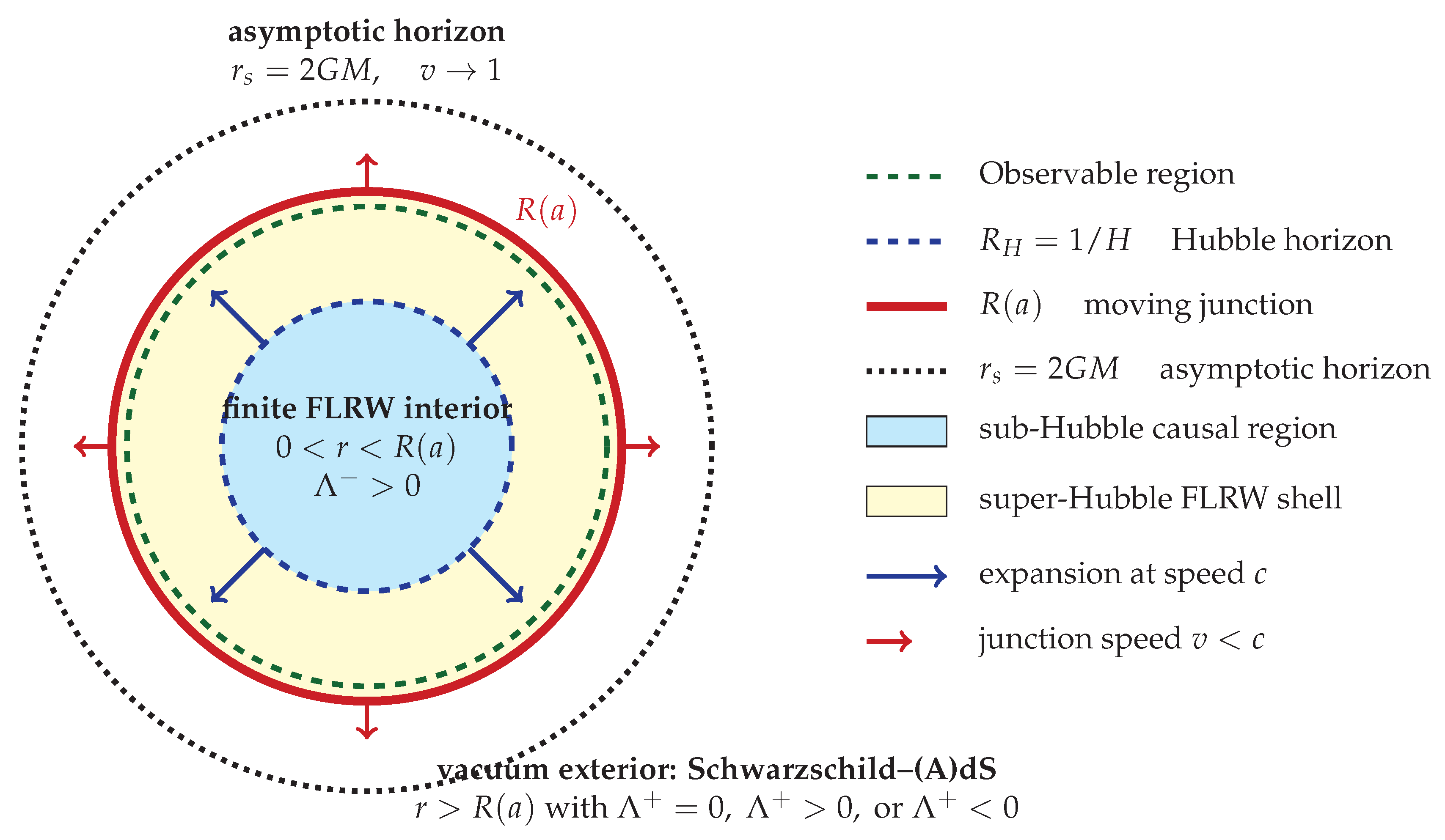
Thus the boundary condition forces the cosmological horizon scale to coincide with the Schwarzschild radius associated with the enclosed mass, $R_{\Lambda -}\simeq r_s$. In other words, the interior FLRW solution requires ${\Lambda }^{-}={\displaystyle \frac{3}{r_s^2}}$, even when the exterior spacetime is asymptotically Minkowski (${\Lambda }^{+}=0$). This solution is illustrated in Figure 1.

The identification $R_{\Lambda -}\simeq r_s$ appears to be a geometric property of the junction dynamics itself rather than a special feature of a particular cosmological model.

4.3. Implications for $\Lambda$

We have found that the variational principle admits a consistent FLRW solution with a non-zero interior cosmological constant. This is a central result of the present work. The fact that ${\Lambda }^{+}\ne {\Lambda }^{-}$ does not imply a discontinuity of either the induced metric or the extrinsic curvature. Continuity follows from the boundary (or matching) junction conditions themselves, which remain satisfied because the matching conditions depend on the geometry of the hypersurface rather than on the individual values of $\Lambda$ appearing in the bulk field equations.

The non-trivial branch therefore, generates an interior cosmological constant ${\Lambda }^{-}={\displaystyle \frac{3}{r_s^2}}$ independently of the exterior ${\Lambda }^{+}$ in the limit $|{\Lambda }^{+}|\ll |{\Lambda }^{-}|$. Within the decomposition introduced in Eq.17, this fixes the required boundary contribution to:

$${\Lambda }_B={\displaystyle \frac{3}{r_s^2}}-{\Lambda }_F-{\Lambda }_G$$

(34)

where ${\Lambda }_F$ and ${\Lambda }_G$ are other possible contributions to $\Lambda$ in Eq.17. This shows how ${\Lambda }_F$ and ${\Lambda }_G$ are cancelled by the boundary term.

The effective cosmological constant ${\Lambda }^{-}$ is inversely proportional to the square of the Schwarzschild radius of the FLRW cloud. For sufficiently large systems, the resulting value is naturally small while remaining non-zero.

In the present framework, we can recover the standard infinite FLRW interpretation as a limiting case by taking $r_s\to \infty$. In this limit, the boundary-selected contribution satisfies ${\Lambda }^{-}\to 0$, so that the boundary contribution disappears and the FLRW region becomes effectively infinite.

Conversely, a finite value of the interior cosmological constant requires $r_s<\infty$. Since the junction condition implies ${\Lambda }^{-}={\displaystyle \frac{3}{r_s^2}}$, the observed non-zero value of ${\Lambda }^{-}$ corresponds, within the present framework, to a finite gravitating FLRW region bounded by a causal horizon.

4.4. Causal Interpretation

The junction radius admits an even more direct causal interpretation. Using Eq.25 together with $R=a\chi$, we obtain

$$a\dot{\chi }=-v.$$

(35)

Thus the comoving position of the junction is determined by

$$\chi \left(\tau \right)=-{\int }_0^{\tau }{\displaystyle \frac{vd\tau }{a\left(\tau \right)}}.$$

(36)

Using the asymptotic boundary condition ${\chi }_{\infty }=0$, this can be equivalently written as

$$\chi \left(a\right)={\int }_a^{\infty }{\displaystyle \frac{vda}{H{a}^2}}.$$

(37)

Therefore

$$R\left(a\right)=a\chi \left(a\right)=a{\int }_a^{\infty }{\displaystyle \frac{v\left(a\right)da}{H{a}^2}}<R_{\Lambda }.$$

(38)

Here $v\left(a\right)$ is the peculiar velocity of the junction hypersurface relative to the local FLRW frame. This expression shows that, once the late-time Friedmann evolution $H\left(a\right)$ is specified, the late-time attractor solution to Eq.27:

$$R\to r_s,v\to 1$$

(39)

is imposed, and the non-comoving branch is uniquely fixed. As the attractor is approached, $v\to 1$, the boundary becomes asymptotically null and converges to the future event horizon.

This provides a geometric interpretation of the variationally selected boundary. It is not an arbitrary matching surface but the unique causal horizon $R\left(a\right)$ generated by the junction dynamics itself. The logical chain can be summarised as:

$$\begin{array}{|c|}\hline \delta S_{\Sigma }=0⟹v\ne 0⟹R\left(a\right)=a{\int }_a^{\infty }{\displaystyle \frac{vda}{H{a}^2}}.\\ \hline\end{array}$$

(40)

The appearance of $R_{\Lambda }=r_s$ is therefore no longer mysterious. It is not imposed as an additional assumption but emerges from the causal structure selected by the variational principle.

The causal-horizon branch identified above also has important implications for gravitational collapse. In particular, the asymptotic condition $R\to r_s$ suggests that trapped regions arise naturally from the boundary dynamics and can persist through both collapsing and expanding phases. This raises the possibility that bounce cosmologies remain inside a trapped region throughout their evolution [14]. A detailed analysis of collapse, bounce dynamics, and their relation to black-hole and white-hole spacetimes will be presented elsewhere.

5. Conclusion

We have shown that requiring a well-defined variational principle for a finite FLRW spacetime matched to an exterior vacuum leads to a unique non-trivial junction solution with important consequences for gravitation and cosmology.

The first main result is that the junction equation admits two qualitatively distinct branches. The familiar comoving branch ($v=0$) reproduces the Oppenheimer–Snyder dust solution and exists only for pressureless matter with vanishing effective cosmological constant. Once radiation or any fluid with non-zero pressure is present, this branch ceases to satisfy the Friedmann evolution and the physically relevant solution is necessarily the non-comoving branch ($v\ne 0$). The boundary remains timelike throughout cosmic history, approaches a null hypersurface asymptotically, and evolves toward the universal attractor

$$H^2+{\displaystyle \frac{1}{R_k^2}}\to {\displaystyle \frac{1}{r_s^2}},$$

independent of the sign of H and valid for open, flat and closed FLRW geometries.

The second main result is that this attractor uniquely fixes the asymptotic boundary radius,

$$R_{\Lambda }=r_s,$$

which immediately implies

$${\Lambda }^{-}={\displaystyle \frac{3}{r_s^2}}.$$

In this framework the observed cosmological constant is therefore not an arbitrary parameter of the Einstein equations but a geometric consequence of the causal boundary selected by the variational principle. The junction radius satisfies

$$R\left(a\right)=a{\int }_a^{\infty }{\displaystyle \frac{vda}{H{a}^2}},$$

showing that the variationally selected boundary is itself a causal horizon generated dynamically by the junction evolution.

A particularly important consequence is that the variational principle remains perfectly well defined even when the effective cosmological constant differs across the junction,

$${\Lambda }^{-}\ne {\Lambda }^{+}.$$

The induced metric and extrinsic curvature remain continuous, so the difference between the two cosmological constants does not represent a physical discontinuity of spacetime. The interior FLRW region and the parent spacetime may therefore possess different effective vacuum energies. The exterior need not be asymptotically de Sitter; it may equally well be asymptotically Minkowski, de Sitter or Anti-de Sitter. This considerably enlarges the class of physically admissible embeddings of finite cosmological regions and may prove relevant to approaches based on holography, string theory or other higher-dimensional constructions, where the natural vacuum of the parent spacetime differs from that observed inside our cosmological domain.

Within the present framework the observable cosmological constant may be decomposed as

$${\Lambda }^{-}={\Lambda }_F+{\Lambda }_G+{\Lambda }_B,$$

where ${\Lambda }_F$ represents possible modifications of the Einstein–Hilbert action, ${\Lambda }_G$ denotes vacuum-energy contributions, and ${\Lambda }_B$ is the boundary contribution fixed by the variational principle. Since the junction condition uniquely determines the total observable value,

$${\Lambda }^{-}={\displaystyle \frac{3}{r_s^2}},$$

the boundary contribution automatically compensates any additional constant terms. In this sense, the cosmological constant problem is reformulated as a boundary-value problem rather than a fine-tuning problem.

The non-comoving branch also provides an exact extension of the Oppenheimer–Snyder interior solution to fluids with non-zero pressure. The solution applies equally to expanding and collapsing phases and to open, flat and closed spatial geometries, demonstrating that General Relativity admits exact FLRW interior solutions beyond the pressureless case. In this sense, the black-hole Universe picture emerges naturally from the variational principle rather than being introduced as an independent assumption.

The standard infinite FLRW solution is recovered in the limit

$$r_s\to \infty ,$$

for which the boundary contribution disappears and ${\Lambda }^{-}\to 0$. Thus, within the present framework, the observed non-zero cosmological constant points naturally to a finite gravitating FLRW region bounded by a causal horizon rather than to an exactly infinite cosmological spacetime.

Finally, although the proper boundary radius asymptotically approaches the finite value $R\to r_s$, the corresponding comoving coordinate satisfies $\chi =R/a\to 0$. This does not signal the formation of a physical singularity. Rather, it reflects the exponential stretching of the FLRW coordinate grid, exactly as occurs when static and expanding coordinate systems are compared in de Sitter spacetime. The attractor is therefore fundamentally a horizon solution rather than a comoving one.

More generally, the present work suggests that observable cosmological parameters may ultimately be determined not only by local field equations but also by the global causal structure selected by the variational principle. If so, the cosmological constant may represent the first example of a physical parameter whose observed value is fixed by the geometry of the finite causal domain in which observations are possible.

An important conceptual consequence concerns the cosmological principle. A finite FLRW region bounded by a causal horizon does not imply a preferred position or observable edge. Since all cosmological observations are restricted to the observer’s past light cone, no present observation can distinguish an infinite FLRW spacetime from a sufficiently large finite FLRW region with identical local matter content. As shown in Appendix B, the causal boundary always remains outside the past light cone of every comoving observer located inside the horizon. Consequently every such observer measures the same homogeneous and isotropic background despite the finite extent of the spacetime.

The boundary therefore reveals itself only indirectly through global causal effects. Within the present framework these include the observed value of the cosmological constant and the existence of a maximum causally connected angular scale [30], rather than any observable anisotropy associated with a physical edge. In this sense the causal boundary enhances large-scale homogeneity rather than violating the cosmological principle.

Appendix A.1. Angular Junction Condition

Using the Christoffel symbols of the two metrics, the angular components of the extrinsic curvature are

$$\begin{array}{cc}\hfill K_{\theta \theta }^{+}& =-\gamma \beta R,\hfill \end{array}$$

(A23)

$$\begin{array}{cc}\hfill K_{\theta \theta }^{-}& =-{\displaystyle \frac{\gamma R}{\sqrt{A}}}\left(A-vHR\right).\hfill \end{array}$$

(A24)

The corresponding azimuthal components satisfy

$$K_{\phi \phi }^{\pm }={sin}^2\theta K_{\theta \theta }^{\pm }.$$

(A25)

Continuity of the angular extrinsic curvature gives

$$\begin{array}{|c|}\hline \beta ={\displaystyle \frac{A-vHR}{\sqrt{A}}}.\\ \hline\end{array}$$

(A26)

Combining Eqs. (A14) and (A26) yields

$$\begin{array}{|c|}\hline {\dot{R}}^2={\displaystyle \frac{{\left(A-vHR\right)}^2}{A}}-sF\left(R\right).\\ \hline\end{array}$$

(A27)

Restoring the original variables, this is

$$\begin{array}{|c|}\hline {\dot{R}}^2={\displaystyle \frac{{\left(1-k{\chi }^2-vHR\right)}^2}{1-k{\chi }^2}}-{\gamma }^{-2}F\left(R\right).\\ \hline\end{array}$$

(A28)

Using the kinematic identity $\dot{R}=HR-v$, Eq. (A27) factorises as

$$\begin{array}{|c|}\hline A{\gamma }^{-2}\left[A-F\left(R\right)-H^2{R}^2\right]=0.\\ \hline\end{array}$$

(A29)

For every finite timelike portion of the junction, $A-v^2>0$, and the angular condition therefore reduces to

$$F\left(R\right)+H^2{R}^2=1-{\displaystyle \frac{k{R}^2}{a^2}}.$$

(A30)

Equivalently,

$$\begin{array}{|c|}\hline H^2+{\displaystyle \frac{k}{a^2}}={\displaystyle \frac{1-F\left(R\right)}{R^2}}.\\ \hline\end{array}$$

(A31)

It is useful to define

$$Q\left(a\right)\equiv H{\left(a\right)}^2+{\displaystyle \frac{k}{a^2}},\mathcal{F}\left(R\right)\equiv {\displaystyle \frac{1-F\left(R\right)}{R^2}}.$$

(A32)

The angular junction condition then takes the simple algebraic form

$$\begin{array}{|c|}\hline Q\left(a\right)=\mathcal{F}\left(R\right).\\ \hline\end{array}$$

(A33)

For a Schwarzschild–de Sitter exterior,

$$F\left(R\right)=1-{\displaystyle \frac{r_s}{R}}-{\displaystyle \frac{{\Lambda }_{+}}{3}}{R}^2,$$

(A34)

Eq. (A31) becomes

$$\begin{array}{|c|}\hline H^2+{\displaystyle \frac{k}{a^2}}={\displaystyle \frac{r_s}{R^3}}+{\displaystyle \frac{{\Lambda }_{+}}{3}}.\\ \hline\end{array}$$

(A35)

This relation is required at every finite timelike point of the junction, independently of whether the junction is comoving or non-comoving.

Appendix A.2. Temporal Junction Condition

The temporal component of the extrinsic curvature does not vanish for a general non-comoving boundary. On the FLRW side, direct calculation gives

$$\begin{array}{|c|}\hline K_{\tau \tau }^{-}=-{\displaystyle \frac{\gamma }{\sqrt{A}}}\left[\dot{v}+Hvs-{\displaystyle \frac{k\chi v^2}{aA}}\right].\\ \hline\end{array}$$

(A36)

Equivalently,

$$K_{\tau \tau }^{-}=-{\displaystyle \frac{\gamma }{\sqrt{A}}}\left[\dot{v}+Hv\left(1-{\displaystyle \frac{v^2}{A}}\right)-{\displaystyle \frac{k\chi v^2}{aA}}\right].$$

(A37)

This component vanishes for a comoving boundary, $v=0$, but it is nonzero in general.

The derivative of s along the junction is

$$\dot{s}=-{\displaystyle \frac{2v}{A}}\left(\dot{v}-{\displaystyle \frac{k\chi v^2}{aA}}\right).$$

(A38)

On the exterior side, the temporal component is

$$\begin{array}{|c|}\hline K_{\tau \tau }^{+}={\displaystyle \frac{\gamma }{\beta }}\left[s\ddot{R}-{\displaystyle \frac{1}{2}}\dot{R}\dot{s}+{\displaystyle \frac{1}{2}}{s}^2{F}_{,R}\left(R\right)\right].\\ \hline\end{array}$$

(A39)

Here

$$F_{,R}\equiv {\displaystyle \frac{dF}{dR}}.$$

(A40)

The exact temporal junction condition is therefore $K_{\tau \tau }^{+}=K_{\tau \tau }^{-}$ in the above equations. Using

$$\ddot{R}=R\dot{H}+H\dot{R}-\dot{v},$$

(A41)

together with Eqs. (A38) and (A26), the temporal condition reduces to

$$\begin{array}{|c|}\hline s\left\{R\dot{H}-{\displaystyle \frac{k\chi v^2}{aA}}+s\left[H^{2}R+{\displaystyle \frac{1}{2}}{F}_{,R}\left(R\right)\right]\right\}=0.\\ \hline\end{array}$$

(A42)

We can see here how the null case limit $s\to 0$ (${\overline{v}}^2\to 1$) is fulfilled trivially (we will later case see in Eq.A48) that $\overline{v}=0$ is also a solution). For a finite timelike junction, $s>0$, and hence

$$R\dot{H}-{\displaystyle \frac{k\chi v^2}{aA}}+s\left[H^{2}R+{\displaystyle \frac{1}{2}}{F}_{,R}\left(R\right)\right]=0.$$

(A43)

In terms of the original variables, this is

$$R\dot{H}-{\displaystyle \frac{k\chi v^2}{a\left(1-k{\chi }^2\right)}}+{\gamma }^{-2}\left[H^{2}R+{\displaystyle \frac{1}{2}}{F}_{,R}\left(R\right)\right]=0.$$

(A44)

Equations (A31) and (A42) are the independent angular and temporal junction conditions for the one-function static exterior Eq. (A9).

Appendix A.3. Combined Form of the Junction Conditions

The angular condition can be written as

$$Q\left(a\right)=\mathcal{F}\left(R\right),$$

(A45)

where Q and $\mathcal{F}$ were defined in Eq. (A32). Differentiating this relation along the trajectory gives

$$2H\left(\dot{H}-{\displaystyle \frac{k}{a^2}}\right)={\mathcal{F}}_{,R}\dot{R}.$$

(A46)

After using Eq. (A33), the left-hand side of Eq. (A42) may be written as

$$-{\displaystyle \frac{svR\left(A-vHR\right)}{2HA}}{\mathcal{F}}_{,R}\left(R\right)=0$$

(A47)

Using Eq. (A26), this is equivalently

$$-{\displaystyle \frac{svR\beta }{2H\sqrt{A}}}{\mathcal{F}}_{,R}\left(R\right)=0$$

(A48)

Consequently, the complete shell-free junction conditions imply

$$\begin{array}{|c|}\hline Q\left(a\right)=\mathcal{F}\left(R\right)\mathrm{and}sv{\mathcal{F}}_{,R}\left(R\right)=0\\ \hline\end{array}$$

(A49)

If we adopt $Q\left(a\right)=\mathcal{F}\left(R\right)$, the first possibility for the additional condition is the comoving branch,

$$v=0,R=a{\chi }_0,$$

(A50)

where ${\chi }_0$ is constant. The second possibility is the null case $s\to 0$. A third possibility would require

$${\mathcal{F}}_{,R}\left(R\right)=0$$

(A51)

along the non-comoving trajectory. For the Schwarzschild–de Sitter exterior,

$$\mathcal{F}\left(R\right)={\displaystyle \frac{r_s}{R^3}}+{\displaystyle \frac{{\Lambda }_{+}}{3}},{\mathcal{F}}_{,R}\left(R\right)=-{\displaystyle \frac{3r_s}{R^4}}.$$

(A52)

Thus, for $r_s\ne 0$, a regular non-comoving timelike junction cannot satisfy both components of the shell-free Israel matching conditions at finite time. The angular condition alone admits a candidate trajectory, but the temporal component remains discontinuous unless the boundary is comoving, we reach the null case $s=0$ in Eq.A42 or a surface stress-energy layer is included [31].

References

- Weinberg, S. The cosmological constant problem. Rev. Mod. Phys. 1989, 61, 1–23. [Google Scholar] [CrossRef]
- Martin, J. Everything You Always Wanted To Know About The Cosmological Constant Problem (But Were Afraid To Ask). Comptes Rendus Phys. 2012, 13, 566–665. [Google Scholar] [CrossRef]
- Padmanabhan, T. A short note on the boundary term for the Hilbert action. Mod. Phys. Lett. A 2014, 29, 1450037. [Google Scholar] [CrossRef]
- Gibbons, G.W.; Hawking, S.W. Action Integrals and Partition Functions in Quantum Gravity. Phys. Rev. D. 1977, 15, 2752–2756. [Google Scholar] [CrossRef]
- Gibbons, G.W.; Hawking, S.W.; Perry, M.J. Path Integrals and the Indefiniteness of the Gravitational Action. Nucl. Phys. B 1978, 138, 141–150. [Google Scholar] [CrossRef]
- York, J.W., Jr. Role of Conformal Three-Geometry in the Dynamics of Gravitation. Phys. Rev. Lett. 1972, 28, 1082–1085. [Google Scholar] [CrossRef]
- Dyer, E.; Hinterbichler, K. Boundary Terms, Variational Principles and Higher Derivative Modified Gravity. Phys. Rev. D. 2009, 79, 024028. [Google Scholar] [CrossRef]
- Oppenheimer, J.R.; Snyder, H. On Continued Gravitational Contraction. Phys. Rev. 1939, 56, 455–459. [Google Scholar] [CrossRef]
- Misner, C.W.; Sharp, D.H. Relativistic Equations for Adiabatic, Spherically Symmetric Gravitational Collapse. Phys. Rev. 1964, 136, B571–B576. [Google Scholar] [CrossRef]
- Faraoni, V. Lemaître model and cosmic mass. General. Relativ. Gravit. 2015, 47(84), 1506.06358. [Google Scholar] [CrossRef]
- Faraoni, V.; Atieh, F. Turning a Newtonian analogy for FLRW cosmology into a relativistic problem. PRD 2020, 102, 044020. [Google Scholar] [CrossRef]
- Gaztañaga, E. How the Big Bang Ends Up Inside a Black Hole. Universe 2022, 8, 257. [Google Scholar] [CrossRef]
- Gaztañaga, E. The Black Hole Universe, part I. Symmetry 2022, 14, 1849. [Google Scholar] [CrossRef]
- Gaztañaga, E.; Kumar, K.S.; Pradhan, S.; Gabler, M. Gravitational bounce from the quantum exclusion principle. Phys. Rev. D. 2025, 111, 103537. [Google Scholar] [CrossRef]
- Gaztañaga, E. The size of our causal Universe. MNRAS 2020, 494, 2766–2772. [Google Scholar] [CrossRef]
- Gaztañaga, E. The cosmological constant as a zero action boundary. MNRAS 2021, 502, 436–444. [Google Scholar] [CrossRef]
- Darmois, G. Les équations de la gravitation einsteinienne; Number 25, 1927. [CrossRef]
- Israel, W. Singular hypersurfaces and thin shells in general relativity. Nuovo Cim. B Ser. 1966, 44, 1–14. [Google Scholar] [CrossRef]
- Poisson, E. A Reformulation of the Barrabes-Israel null shell formalism. arXiv 2002. [Google Scholar]
- Einstein, A. Kosmologische Betrachtungen zur allgemeinen Relativitätstheorie. S.K. Preußischen Akad. Der W. 1917, 142–152. [Google Scholar] [CrossRef]
- Planck Collaboration. Planck 2018 results. VI. Cosmological parameters. A A 2020, A6. [Google Scholar] [CrossRef]
- Calabrese, E.; The Atacama Cosmology Telescope collaboration; T. The Atacama Cosmology Telescope: DR6 constraints on extended cosmological models. JCAP 2025, 2025, 063. [Google Scholar] [CrossRef]
- Lemaitre, G. The expanding universe. Ann. Soc. Sci. Brux. A 1933, 53, 51–85. [Google Scholar] [CrossRef]
- Friedmann, A. Über die Krümmung des Raumes. Z. Fur Phys. 1922, 10, 377–386. [Google Scholar] [CrossRef]
- Lemaître, G. Expansion of the universe, A homogeneous universe of constant mass and increasing radius accounting for the radial velocity of extra-galactic nebulae. MNRAS 1931, 91, 483–490. [Google Scholar] [CrossRef]
- Tolman, R.C. Effect of Inhomogeneity on Cosmological Models. Proc. Natl. Acad. Sci. 1934, 20, 169–176. [Google Scholar] [CrossRef] [PubMed]
- Misner, C.W.; Sharp, D.H. Relativistic Equations for Adiabatic, Spherically Symmetric Gravitational Collapse. Phys. Rev. 1964, 136, 571. [Google Scholar] [CrossRef]
- Easson, D.A. Obstructions to Minimal Regular Black Hole Cosmologies. arXiv 2026. [Google Scholar]
- Camacho-Quevedo, B.; Gaztañaga, E. A measurement of the scale of homogeneity in the early Universe. JCAP 2022, 2022, 044. [Google Scholar] [CrossRef]
- Blau, S.K.; Guendelman, E.I.; Guth, A.H. Dynamics of false-vacuum bubbles. PhyRevD 1987, 35, 1747–1766. [Google Scholar] [CrossRef] [PubMed]
Figure 1.
Schematic representation of the variationally selected FLRW* boundary solution. The full region inside the moving junction is described by the FLRW metric. The inner blue region denotes the sub-Hubble causal domain , while the yellow shell between and is still part of the FLRW interior but lies outside the instantaneous Hubble horizon. This super-Hubble region contains frozen large-scale modes, including the largest observable CMB multipoles. The moving junction remains timelike for finite cosmic time, , and asymptotically approaches the null surface as . Outside the junction lies vacuum spacetime, which may be asymptotically Minkowski, deSitter, or Anti-deSitter. The boundary is not directly observable from inside the FLRW region, but its causal effect appears as the effective interior cosmological constant .
Disclaimer/Publisher’s Note: The statements, opinions and data contained in all publications are solely those of the individual author(s) and contributor(s) and not of MDPI and/or the editor(s). MDPI and/or the editor(s) disclaim responsibility for any injury to people or property resulting from any ideas, methods, instructions or products referred to in the content. |
© 2026 by the authors. Licensee MDPI, Basel, Switzerland. This article is an open access article distributed under the terms and conditions of the Creative Commons Attribution (CC BY) license (http://creativecommons.org/licenses/by/4.0/).
Copyright: This open access article is published under a Creative Commons CC BY 4.0 license, which permit the free download, distribution, and reuse, provided that the author and preprint are cited in any reuse.