
Submitted:
05 July 2026
Posted:
06 July 2026
You are already at the latest version
Abstract
Modern ion-therapy facilities are usually equipped with rotating gantries to achieve higher dose-conformity to the tumor. The gantry is the terminating part of a beam transfer-line (shortly a beamline) from the accelerator to a gantry treatment room. The gantry is mechanically rotated around the patient. In synchrotron-based facilities, the slowly extracted beams have different emittance patterns in the two transverse planes (shortly the asymmetric beams). Several matching techniques were developed in the past to remove the angular dependence of the beam parameters at the irradiation place on the gantry rotation angle. Recently, a novel so-called rotatorlike gantry optics has been introduced. In this concept, all existing matching techniques are integrated into the gantry optics and the gantry nozzle. The underlying theoretical description of its working principle is presented in this paper. It is based on the first-order matrix analysis of the transport of asymmetric beams in rotating ion-optical systems, in general. The results are formulated in terms of ion-optical constraints imposed on the fixed incoming beamline, and the gantry transfer matrix. Theoretical matrix analysis is followed by a design study applied to the MedAustron proton-gantry layout as a typical representative of an isocentric gantry equipped with a pencil-beam scanning system.
Keywords:
accelerator physics
; beam transport
; ion-optics
; ion therapy
; rotating gantry
1. Introduction
High-energy proton (≈60 ÷ 250 MeV) and ion (usually carbon ion, ≈100 ÷ 400 MeV/A) beams have favorable physical and biological characteristics for the treatment of cancer. However, full exploitation of all potential ion-therapy benefits on clinical scale is only possible when the favorable characteristics of ion-therapy beams are supported and accompanied – among other disciplines – by technological development of suitable accelerators, proper beam delivery techniques, and corresponding beam delivery instrumentation [1]. The accelerators must be extremely stable, reliable, and easy to operate, especially when talking about accelerators operated in hospitals out of reach of accelerator physicists and in-house maintenance facilities. Development of the beam delivery systems started from passive beam delivery systems [2] and has progressed to active beam delivery systems [3]. The active beam delivery systems are based on active energy variation and pencil-beam scanning incorporated into rotating gantries. Such a combination provides the best possibilities for optimizing the distribution of the dose delivered to the tumor. On the other hand, it is the most complex and demanding beam delivery instrumentation from the beam transport point of view. It is true especially when the scanning system is located upstream of the last gantry bending magnet (shortly the upstream scanning, e.g., [4,5,6,7,8,9,10]).
The active energy variation can be best performed by a synchrotron. A synchrotron is also the preferred choice for carbon-ion therapy facilities since the energies needed for carbon-ion therapy are too high for cyclotrons. Due to the slow extraction, synchrotrons serve the beams with different transverse emittances and emittance diagrams in the horizontal and vertical plane (shortly the asymmetric beams). This problem has been known for almost three decades [11,12,13,14,15,16,17]. During this time, several matching strategies and techniques have been developed and applied for transport of asymmetric beams in rotating gantries (see for example Refs. [11,16,18,19,20,21,22,23,24] and references therein). They all aim at removing the dependence of the relevant beam parameters at the irradiation place on the gantry rotation angle. Recently, a novel ion-optical concept has been introduced that combines the known matching techniques and integrates them into the gantry optics and the gantry nozzle [25]. It is referred to as the rotatorlike gantry optics. This optics provides the best beam transport of asymmetric beams in terms of equalizing the beam emittances and beam parameters at the irradiation place (usually, but not necessarily, at the gantry isocenter) in the two gantry transverse planes. It also keeps them fully independent from the gantry rotation angle. The beam sizes and the beam position-to-angle correlations in the two gantry transverse planes are matched by ion-optical means. The beam divergence and the beam emittance are balanced with the aid of beam scattering in the gantry nozzle. The physics of beam scattering in gantry nozzles can be found in Refs. [26,27]. Thus, the rotatorlike optical concept requires no additional devices like a rotator or a dedicated scattering foil.
Because the rotatorlike gantry concept is new, the underlying theoretical description of its working principle is presented in this paper in a comprehensive and systematic way. The theoretical description is based on the first-order matrix analysis of the transport of asymmetric beams in rotating ion-optical systems, in general. The results are formulated in terms of ion-optical constraints imposed on the fixed incoming beamline, and the required format of the gantry transfer matrix. Results of the theoretical analysis have been successfully applied to the proton gantry at MedAustron facility [24,25,28,29]. The chosen gantry type represents a typical isocentric barrel upstream 2D quasi-parallel scanning gantry using warm magnets. An in-depth ion-optical design study of the rotatorlike gantry optics working in two imaging modes (point-to-point and parallel-to-point) is presented in this paper. This study can serve as a guideline also for other gantry designers working on angularly independent beam transport in similar gantry types.
2. Materials and Methods
The first-order matrix ion-optical formalisms has been employed as the main method in this paper. The matrix analysis of the rotatorlike gantry optics is based on linear beam dynamics (linear optics), as it is formulated in standard accelerator physics textbooks (e.g., [30,31,32]). These references shall also be consulted concerning details on beam sigma-matrix and Twiss formalisms.
A single-particle trajectory is described with the aid of the particle coordinate vector , where is the horizontal particle position, is the vertical particle position, is the longitudinal path-length difference, and is the relative momentum deviation with respect to the reference momentum, The particle coordinate vector is given in a local rectangular right-handed coordinate system . In this coordinate system, s is the cumulative longitudinal coordinate along the design orbit, stands for the ion-optical horizontal plane, and stands for the ion-optical vertical plane. The ion-optical horizontal plane generally coincides with the bending plane of the dipoles. In the case of the gantry, it coincides with the bending plane of the gantry dipoles and bears no relation to the gantry rotation angle. The gantry rotation angle, , is defined as the angle between the local coordinate system of the incoming fixed beamline the gantry is connected to, and the local coordinate system of the gantry that rotates together with the gantry. Anticlockwise rotation stands for positive angles. It should be noted that the absolute gantry rotation angle in the treatment room may be defined differently by medical physicists. The ion-optical vertical plane is the plane perpendicular to the ion-optical horizontal plane.
The beam is characterized by the beam sigma-matrix (shortly the sigma-matrix). In the case of the uncoupled optics (, ), the sigma-matrix terms can be converted also to the Twiss parameters. The emittance is assumed to be 1rms geometrical emittance defined as the area of the emittance diagram in the phase space divided by . More strictly speaking, the 1rms geometrical emittance is the area (divided by ) of the ellipse matched to the full beam emittance diagram in the phase space containing 39% of the beam particles [33,34]. Definition of the 1rms geometrical emittance is illustrated in Figure 1. It shows an example of a particle distribution (in the vertical phase space) at 5rms cutoff of Gaussian distribution (orange), and the corresponding 1rms ellipse (blue). The emittance diagram has been generated by the WinAGILE computer code [35,36,37].
It shall be noted that the last two terms of the particle coordinate vector, the longitudinal path-length difference, , and the relative momentum deviation, , are not necessary for the matrix analysis presented in this work. Thus, the matrix analysis can be restricted to 4 × 4 matrices, which is enough for the: (i) theoretical analysis of the problem; (ii) description and explanation of the working principle of the rotatorlike gantry optics; (iii) deriving the corresponding ion-optical constraints imposed on the incoming fixed beamline and the gantry transfer-matrix format. However, the beam transport simulations are performed with full 6 × 6 transfer matrices, which is a default setting of the WinAGILE code.
Finally, the gantry is characterized by its first-order transfer matrix in the gantry local coordinate system taken from the gantry entrance to the gantry isocenter.
Following the detailed theoretical analysis, the MedAustron proton gantry has been chosen as a reference. It is a typical representative of an isocentric barrel gantry equipped with a 2D quasi-parallel pencil-beam scanning system located upstream of the last 90° gantry dipole. Moreover, some of the theoretical results presented in this paper have already been implemented and experimentally tested in the MedAustron gantry beamline [24]. A cross-section of the gantry beamline through its bending midplane (the horizontal plane of the gantry local coordinate system) is shown in Figure 2.
The configuration and the main parameters of the gantry beam transport system are summarized in Table 1.
The gantry beam transport system consists of three dipoles and seven quadrupoles. The first two 58° dipoles are identical but bend the beam in the opposite direction. The last 90° dipole has a large aperture to accommodate the scanned beam. The scanning field is 20 cm × 12 cm (horizontally × vertically). The scanning magnets are located at the focal points of the last 90° dipole to perform quasi-parallel scanning. The position of the focal points is adjusted by the last dipole edge focusing. The quadrupoles are physically identical but have different strengths. The quadrupole strengths quoted in Table 1 correspond to the parallel-to-point gantry with magnification of 3.1 m (in both gantry transverse planes) that is presently in clinical operation at the MedAustron therapy center [24]. Its full 6 × 6 transfer matrix, , is listed in Equation (1). The numbers are given in SI units and are rounded to three decimal places. The transfer matrix is calculated by WinAGILE. The term corresponds to the beam kinetic energy of 252.7 MeV, which is the maximum proton beam energy used for the treatments at MedAustron. The gantry transfer matrix reads:
The drift spaces in the gantry lattice are occupied by auxiliary beam transport equipment like beam-profile monitors (SFX), orbit correctors, and scanning magnets. This equipment is listed in Table 1, too. The last drift space downstream of the 90° dipole is occupied by the gantry nozzle. The nozzle starts from the vacuum window that terminates the vacuum chamber of the last 90° dipole. The vacuum window consists of two identical pairs of aluminum and Hostaphan® Polyester foils. The thickness of the Al-foil and the Hostaphan® foil is 5 µm and 190 µm, respectively. There is an evacuated gap of 14 mm between the two Al-Hostaphan® vacuum windows. Downstream of the vacuum window, the nozzle hosts three main beam monitors (in the beam direction): an independent termination system and intensity monitor (ITS), the DDS monitor box 2, and the DDS monitor box 1. Each monitor consists of thin aluminum, Mylar, or Kapton foils and is filled with nitrogen gas. There is also a nozzle exit window made of Kapton. There are air gaps between the vacuum window and the ITS monitor as well as between the ITS and the DDM monitors. Finally, there is an air gap of about 75 cm from the DDS monitor box 1 to the patient. The nozzle length is about 43 cm. Further details concerning the gantry nozzle can be found in Ref. [24].
3. Working Principle of the Rotatorlike Gantry Optics
3.1. General Transformations of the Beam Sigma-Matrix
Rotatorlike matching can be interpreted as a combination of sigma matching and rotator matching, but also as an extended version of the sigma matching [25]. Both interpretations are correct. A characteristic feature of the sigma matching is that the matching is subdivided between the fixed incoming beamline and the gantry. To explain the role of the fixed incoming beam line and the gantry, let us start with general transformations of the sigma-matrix at the gantry entrance, and at the gantry isocenter.
At the fixed beamline exit (FLEX), the beam is described by the beam sigma-matrix, :
where the terms of the beam sigma-matrix represent the covariance of the quantities indicated in brackets. No correlation between the horizontal and vertical plane is assumed in the incoming beam, which corresponds to the coupling-free fixed-beamline optics. In such a case, the beam sigma-matrix can also be expressed in terms of the Twiss parameters:
where , and is the 1rms horizontal and vertical emittance, respectively, and , and are the so-called Twiss parameters. The Twiss parameters in the horizontal plane are indicated by subscript “h”, the Twiss parameters in the vertical plane are indicated by subscript “v”. In each of the two transverse planes, the Twiss parameters obey the relation:
An asymmetric beam is characterized by (essentially) different horizontal and vertical geometrical beam emittances, , and :
Let us now calculate the beam sigma-matrix at the gantry entrance, (GEN), in the gantry local coordinate system, , for a gantry rotation angle, . It is obtained via the transformation [30,31,32]:
where the first matrix from the left is the transfer matrix of the coordinate system rotation by the gantry rotation angle, . Let us denote the terms of the sigma-matrix, , as . Performing the matrix multiplication (6) yields the following set of results:
Notation is just a shortened version of and it is going to be used also in other similar situations through this paper.
Let us assume now an achromatic gantry characterized by its first-order transfer matrix, :
Similarly to the incoming fixed beamline, no coupling between the horizontal and vertical plane is assumed in the gantry optics. Let us define two versions of the gantry optics according to the imaging mode. The point-to-point imaging gantry optics is characterized by . The parallel-to-point imaging gantry optics is characterized by .
The beam sigma-matrix at the gantry isocenter (ISO), , containing the terms is obtained via the transformation:
Performing the matrix multiplication (9) yields the following list of the beam sigma-matrix terms at the gantry isocenter in its general form:
At this point, one can formulate the constraints the matching of the asymmetric beams is aiming at. At the gantry isocenter, the following conditions shall be fulfilled:
The first condition is equivalent to the same 1rms beam size in the two gantry transverse planes that is independent from the gantry rotation angle, . The round beam, , is a fundamental requirement of medical physicists. Its independence from the gantry rotation angle makes it possible to operate the gantry with the same ion-optical setting at all gantry angles, thus contributing to simplicity and reliability of gantry operation.
The second condition is equivalent to the same and rotationally independent position-to-angle covariances in the two gantry transverse planes. Although it is not directly a part of medical specifications, the ion-optical profit from this specific feature has been thoroughly discussed in Ref. [25]. It has been shown in this reference that, when this condition is fulfilled, the shape of the beam envelopes in the gantry nozzle can be effectively controlled.
Finally, the third condition guarantees the round beam spot without horizontal-to-vertical covariance in the real space at the gantry isocenter.
Asking simultaneously for the same and rotationally independent beam divergence () would result in the same horizontal and vertical beam emittance, , which is not possible for the asymmetric beams. Nevertheless, this is of less concern because the beam divergence as calculated by the ion optics is going to be essentially altered by the beam scattering in the gantry nozzle including the emittance blowup [26,27]. If the beam is properly served to the gantry nozzle, the beam scattering can practically entirely equalize the emittance diagrams in the two gantry transverse planes at the gantry isocenter [25].
If the beam waist is required at the gantry isocenter, the second condition becomes stricter:
Satisfying the set of conditions (11) or (12) requires some cooperation between the fixed incoming beamline and the gantry to eliminate the gantry rotation angle from the pertinent sigma-matrix terms at the gantry isocenter, , (see the set of Equation (10)). As stated above at the beginning of this section, the matching must be subdivided between the fixed incoming beamline and the gantry.
3.2. The Matching Role of the Fixed Incoming Beamline
Let us consider three pairs of the sigma-matrix terms at the fixed beamline exit, , and . These pairs are composed of the equivalent sigma-matrix terms, the first term always corresponds to the horizontal plane, and the second one to the vertical plane. Beam asymmetry makes it possible to equalize the terms in any two pairs out of those three. The terms in the third pair must then be necessarily different. In other words, one can “move” the whole beam asymmetry into one of the above listed pairs (any of them, shortly the asymmetric pair) while keeping the other two balanced. The situation is illustrated in Table 2.
Figure 3 illustrates the matching role of the fixed incoming beamline graphically. It shows how the beam must be served/prepared at the fixed beamline exit. For this purpose, “a unit beam” in the vertical plane is assumed. Its parameters in the vertical plane are mm⋅mrad, m, and . The corresponding 1rms beam parameters are mm (the 1rms beam size), and mrad (the 1rms beam divergence). The emittance diagram of such a beam in the vertical plane has been shown in Figure 1.
In the horizontal plane of the fixed incoming beamline, the emittance diagram is expected to be a bar-of-charge-like narrow strip (shortly the bar) [24,25]. In this paper, the emittance diagram in the horizontal plane is going to be represented by a bar-thin ellipse with 1rms geometrical emittance of mm⋅mrad. Its Twiss parameters and the sigma-matrix terms will depend on its orientation with respect to the full ellipse. They must be calculated individually for each mode listed in Table 2. This is shown in Table 3. Note that the beam parameters in the vertical plane are frozen for all three HEBT modes, whereas the beam parameters in the horizontal plane depend on the matching mode.
In mode I (the red emittance diagram in Figure 3), the beam has the same 1rms beam size and position-to-angle covariance in the two transverse planes, the beam divergence must then be necessarily different. In mode II (the yellow emittance diagram in Figure 3), the beam has the same 1rms beam divergence and position-to-angle covariance in the two transverse planes, the beam size must be different. Finally, in mode III, the beam has the same 1rms beam size and 1rms beam divergence in the two transverse planes, the position-to-angle covariance must be different. In this case, there are two beams like that with opposite sign of . The light-green emittance diagram in Figure 3 corresponds to positive , the dark-green emittance diagram in Figure 3 corresponds to negative .
3.3. The Matching Role of the Gantry
When the beam at the fixed beamline exit is prepared according to Table 2, eliminating the angular dependence from the relevant sigma-matrix terms at the gantry isocenter is feasible with the following gantry transfer matrices [11,16]:
in mode I, and:
in mode II. The transfer matrices (13) and (14) correspond to the point-to-point and parallel-to-point imaging mode, respectively. The unit determinant of the horizontal and vertical submatrices is already taken into account.
3.3.1. The Sigma-Matching in Mode I and Mode II
In mode I, plugging , , and into the set of Equation (10) yields:
There are only three beam parameters at the gantry isocenter that remain a function of the gantry rotation angle, namely the horizontal beam divergence, , the vertical beam divergence, , and the covariance between them, . They are all related to beam divergence, which is in accordance with our design strategy. The beam divergence as determined by ion optics is of minor concern because it is going to be essentially altered by beam scattering at the gantry nozzle. This scattering can even be used to equalize the horizontal and vertical beam emittances and divergences at the gantry isocenter by proper adjustment of the emittance diagrams at the vacuum window [25].
Similarly, in mode II, plugging , , and into the set of Equation (10) yields:
The results of the sigma-matching presented by the set of Equations (15) and (16) show, which beam parameters in the two transverse planes at the gantry isocenter can be made independent from the gantry rotation angle by ion-optical means. In both cases, it is the beam size, and the position-to-angle covariance. So far, the constraints and have not been applied yet. A beam with and is probably of small interest for treatments, but it may be useful for the diagnostics of the gantry optics. For treatments, a round beam and is preferred. Satisfying these additional constraints is equivalent to the matching goal as formulated by the set of Equation (11) and can be achieved in two different ways. One of them leads to the rotatorlike gantry optics as it is going to be derived in Section 4. However, before progressing to that section, let us complete first the matrix analysis for the HEBT mode III, too.
3.3.2. The Sigma-Matching in Mode III
In mode III, plugging , , and into the set of Equation (10) yields:
Similarly, plugging , , and into the set of Equation (10) yields:
It can be seen that both gantry imaging modes (point-to-point as well as parallel-to-point) fail in satisfying the set of constraints (11), namely in satisfying . This is because at the HEBT exit. That is why this matching mode has been excluded from further analysis and design studies.
4. Results
4.1. From Sigma-Matching to the Rotatorlike Gantry Optics
Let us now ask not just for the rotation independent beam-size at the gantry isocenter, but also for the same beam-size in the horizontal and vertical plane of the gantry, . Similarly, let us require in addition to and .
4.1.1. The Point-to-Point Imaging Mode (Mode I)
In mode I, the equal beam-size constraint means (see the set of Equations (15)):
which is satisfied either with or (shortly ).
The equal position-to-angle covariance means:
The unit transfer-matrix determinant, , simplifies Equation (20) to:
Combination of Equation (19) with Equation (21) yields two possible point-to-point imaging gantry transfer matrices:
or
4.1.2. The Parallel-to-Point Imaging Mode (Mode II)
The transfer matrices for the parallel-to-point imaging mode can be derived from mode II exactly in the same manner:
or
The transfer matrices (22) and (24) represent a mathematically trivial case with entirely identical horizontal and vertical submatrices. In the transfer matrices (23) and (25), the vertical submatrix is the sign-reversed horizontal submatrix, which is the rotatorlike matrix format [15,18,19,20,24]. These matrices combine the sigma-matching with the rotator-matching, thus providing unique and attractive matching features. The rotatorlike gantry optics makes it possible to form beam waists at the gantry isocenter by adjusting the position-to-angle covariance at the gantry entrance. In addition, it makes beam scattering in the gantry nozzle fully independent from the gantry rotation angle. The beam waists at the gantry isocenter are achieved by setting . Required input covariance can be calculated from Equation (20). The rotation-independent beam scattering is guaranteed by the fact that the rotatorlike optics rotates the beam at the vacuum window by the gantry rotation angle. This is a direct consequence of the rotator working principle. Its mathematical proof can be found in Ref. [25]. Thus, the scattering always starts at the vacuum window for all gantry rotation angles from the same emittance pattern. The scattered beam spot at the gantry isocenter rotates together with the gantry rotation. If the scattered beam spot at the gantry isocenter is round, this rotation can be ignored, which has been experimentally verified and reported in [24].
4.2. A Design Study of the Rotatorlike Gantry Optics
The above derived theoretical results have been applied to the MedAustron proton gantry that has been chosen as a reference gantry. The gantry optics has been tuned to both the point-to-point imaging mode (transfer matrix according to Equation (23)) as well as to the parallel-to-point imaging mode (transfer matrix according to Equation (25)). In each imaging mode, the gantry transfer matrix was tuned to different magnifications. The beam transport in the gantry has been investigated systematically as a function of the gantry magnification. The required beam parameters at the gantry isocenter were set according to medical and ion-optical specifications as defined at MedAustron [24]. At the gantry isocenter, a round beam of more than 6 mm (FWHM) is requested, waists in both transverse planes. The gantry optics must be achromatic and independent from the gantry rotation angle. Keeping in mind the additional contribution from beam scattering, we set the beam size as formed by ion optics (i.e., without scattering) to 6 mm FWHM. The technological limit for the quadrupole power converters was set to m-1, where is the normalized quadrupole strength, and is the quadrupole effective length ( cm).
4.2.1. The Point-to-Point Imaging Gantry
The gantry-optics design study started from the point-to-point rotatorlike imaging mode. The gantry transfer matrix has been matched to:
where is the gantry magnification. For matching purposes, the Twiss parameters at the gantry entrance in both gantry transverse planes were set to m and . The transfer matrix (26) can be then achieved with the horizontal phase advance , vertical phase advance , and equal exit alphas . Exit betas must be constrained according to the required gantry magnification, . In addition to this, zero dispersion and its first derivatives are constrained at the gantry isocenter (the same is assumed for the dispersion function at the gantry entrance).
For each gantry magnification, , the full-ellipse input Twiss parameters are calculated first as follows:
where mm and mm⋅mrad,
where Equation (20) has been used considering output waists (. Equations (27) and (28) make it possible to calculate the full-ellipse Twiss parameters at the gantry entrance as a function of the required beam size at the gantry isocenter, , and the gantry magnification, . The term of the gantry transfer matrix depends on the gantry magnification. It must be obtained as a product of fitting the gantry transfer matrix to the desired format given by Equation (26).
The input Twiss parameters for the bar-thin ellipse are obtained by scaling the above full-ellipse input Twiss parameters to satisfy , and . This scaling yields:
where the full ellipse is assumed to be in the vertical plane whereas the bar-thin ellipse is in the horizontal plane, mm⋅mrad. Both Twiss parameters, beta and alpha, are simply scaled with the emittance ratio (see also the first column of Table 2).
Figure 4 shows the results of fitting in terms of quadrupole excitations as a function of the gantry magnification.
The point-to-point rotatorlike gantry can be operated with magnification ranging from about 0.8 to about 2.2 (accurately from 0.777 to 2.183). The exact values were obtained by setting the pertinent quadrupoles to the maximum possible strength and fitting just equal output betas instead of specifying any concrete output-beta value. The pertinent quadrupoles were not used as fitting variables in these fits. One fitting was done with setting the first quadrupole Q1 to m-2, another one with setting the fourth quadrupole Q4 to m-2. The resulting data points are indicated with the enlarged markers in Figure 4. Outside the magnification interval , the quadrupoles Q1 and Q4 exceed the technological limit of m-1, respectively.
In the next step, beam envelopes inside the gantry have been checked for all gantry magnifications indicated in Figure 4. Figure 5 shows the FWHM beam envelopes (2.3548rms beam half-width) for the gantry magnification , which represents the middle of the feasible magnification interval. The input beam parameters correspond to the beam mm at the gantry isocenter, waists. They were calculated according to Equations (27)–(30). The beam envelopes were calculated with the aid of the WinAGILE code including the dispersion contribution in the horizontal plane of the gantry for (the dispersion function is going to be shown in the next Chapter).
As it can be seen in Figure 5, the rotatorlike optics works as expected. The beam parameters at the gantry isocenter are in accordance with the results of the matrix analysis. They are also independent from the gantry rotation angle, which is demonstrated by two significant gantry angles, 0° and 90°. Figure 6 shows the emittance diagrams at the HEBT exit (upper row) and at the gantry isocenter (lower row). The emittance diagrams at the HEBT exit were generated by the WinAGILE code. Subsequently, they were tracked through the gantry beamline by the WinAGILE “tracking distributions” routine. The 1rms cut-off is provided to demonstrate the HEBT matching role and the sigma-matched beam parameters at the gantry isocenter.
Checking the beam envelopes inside the gantry is of crucial importance to avoid beam scraping by the vacuum chamber walls. The beam envelopes inside the point-to-point rotatorlike gantry exhibit a pronounced peak in the vertical plane downstream to the first 58° gantry dipole (see Figure 5). This is an unfavorable position because the dipole vacuum chamber is vertically narrow. The height of this peak depends on the gantry magnification as shown in Figure 7 together with the full-ellipse input Twiss parameters at the gantry entrance calculated according to Equations (27) and (28).
4.2.2. The Parallel-to-Point Imaging Gantry
In the parallel-to-point rotatorlike imaging mode, the gantry transfer matrix has been matched to:
where is the gantry magnification. For matching purposes, the Twiss parameters at the gantry entrance in both gantry transverse planes were set to m and . The transfer matrix (31) has been then achieved with the horizontal phase advance , vertical phase advance , and equal exit alphas . Exit betas must be constrained according to the required gantry magnification, . Since m and , m-1. In addition to this, zero dispersion and its first derivatives are constrained at the gantry isocenter (the same is assumed for the dispersion function at the gantry entrance). It should be pointed out that WinAGILE does not allow entering the -parameter directly. That is why all Twiss entries for WinAGILE must be converted to betas and alphas.
Similarly, as in case of the point-to-point rotatorlike imaging mode, for each gantry magnification, , the full-ellipse input Twiss parameters are calculated first as follows:
where mm and mm⋅mrad,
where term of the gantry transfer matrix depends on the gantry magnification and must be obtained as a product of fitting the gantry transfer matrix to the desired format given by Equation (31). The input beta required as a WinAGILE entry is calculated from relation (4).
The input Twiss parameters for the bar-thin ellipse are obtained by scaling the above full-ellipse input Twiss parameters to satisfy , and . This scaling yields:
where the full ellipse is assumed to be in the vertical plane whereas the bar-thin ellipse is in the horizontal plane, mm⋅mrad. The Twiss parameters gamma and alpha are simply scaled with the emittance ratio (see also the second column of Table 2). Note that due to the parallel-to-point imaging mode, Equations (34) and (35) are equivalent to Equations (29) and (30) with beta being interchanged with gamma.
Figure 8 shows the results of fitting in terms of quadrupole excitations as a function of the gantry magnification.
The parallel-to-point rotatorlike gantry can be operated with magnification ranging from about 1.3 m to about 5.2 m (accurately from 1.325 m to 5.229 m). The exact values were obtained by setting the pertinent quadrupoles to the maximum possible strength and fitting just equal output betas instead of specifying any concrete output-beta value. The pertinent quadrupoles were not used as fitting variables in these fits. One fitting was done with setting the first quadrupole Q1 to m-2, another one with setting the sixth quadrupole Q6 to m-2. The resulting data points are indicated with the enlarged markers in Figure 8. Outside the magnification interval m, the quadrupoles Q1 and Q6 exceed the technological limit of m-1, respectively.
In the next step, beam envelopes inside the gantry have been checked for all gantry magnifications indicated in Figure 8. Figure 9 shows the FWHM beam envelopes (2.3548rms beam half-width) for the modest gantry magnification m, which represents approximately the middle of the feasible magnification interval. The input beam parameters correspond to the beam mm at the gantry isocenter, waists. They were calculated according to Equations (32)–(35). The beam envelopes were calculated with the aid of the WinAGILE code including the dispersion contribution in the horizontal plane of the gantry for .
The beam parameters at the gantry isocenter are in accordance with the results of the matrix analysis. They are also independent from the gantry rotation angle, which is demonstrated by two significant gantry angles, 0° and 90°. Figure 10 shows the emittance diagrams at the HEBT exit (upper row) and at the gantry isocenter (lower row). The emittance diagrams at the HEBT exit were generated by the WinAGILE code. Subsequently, they were tracked through the gantry beamline by the WinAGILE “tracking distributions” routine. The 1rms cut-off is provided to demonstrate the HEBT matching role and the sigma-matched beam parameters at the gantry isocenter.
The beam envelopes inside the parallel-to-point rotatorlike gantry exhibit also a pronounced peak in the vertical plane behind the first 58° gantry dipole like the point-point rotatorlike gantry, but it is much lower than the peak in the point-to-point gantry (compare Figure 5 with Figure 9). Especially in the magnification interval from 2.0 m to 2.5 m, the vertical envelope-maximum is about 11 mm in case of the parallel-to-point rotatorlike gantry versus 18 mm in case of the point-to-point rotatorlike gantry with magnification 0.9. At magnifications over 5.0 m, the vertical envelope-maximum moves to a different position upstream of the first 58° gantry dipole. This is manifested by the change of the trend of the pertinent (blue) curve in Figure 11 that shows the full-ellipse input Twiss parameters at the gantry entrance together with the maximum of the beam envelope as a function of the gantry magnification.
5. Discussion
5.1. The Waist-to-Waist Imaging
The parallel-to-point rotatorlike gantry optics turned out to be superior to the point-to-point optics thanks to the following important general features:
- Significantly smaller beam envelopes inside the gantry;
- A significantly larger interval of feasible gantry magnifications;
- The waist-to-waist beam-transport mode possible within the feasible interval of gantry magnifications.
As it can be seen in Figure 11, there is one specific gantry magnification when the input Twiss parameter alpha is zero (in both gantry planes). This magnification has been found by running the matching routine with input betas 1 m, input alphas zero and asking for the output alphas to be zero while output betas being equal in the vertical and horizontal gantry plane without specifying any concrete value for them. Other matching constraints are the same as for matching the parallel-to-point rotatorlike transfer matrix format. The result of matching yielded the gantry magnification m. The corresponding 4 × 4 gantry transfer matrix reads (the transfer-matrix terms are given in SI units and rounded to four decimal digits):
The waist-to-waist beam-transport mode is exclusively a property of the gantry transfer matrix, which means that it is independent from the choice of the beam FWHM at the gantry isocenter. It should be noticed that the waist-to-waist option is not available in the point-to-point gantry imaging mode within the feasible magnification interval (see Figure 7). The beam waists at the gantry entrance turned out to be advantageous for the beam transport inside the HEBT. That is why the waist-to-waist parallel-to-point imaging mode has been selected as the final candidate for the gantry optics. Figure 12 shows the beam envelopes for the optimized gantry magnification of 2.5027 m in the waist-to-waist mode (red and blue) and compares them to the presently used setting with the gantry magnification of 3.10 m (black). The present setting runs with the input Twiss parameters at the gantry entrance , where the horizontal and vertical plane is related to the HEBT coordinate system.
The waist-to-waist mode has been recently implemented as a part of the gantry-beamline recommissioning. The presented design study was run for an amended medical-physics specification of beam size at gantry isocenter , which is shown in Figure 13. The measured data confirms the beam-transport calculations.
5.2. Achromatic Beam Transport
It is rather interesting to see the ion-optical flexibility of the gantry beamline despite of the fact that only two out of seven quadrupoles are located in a dispersion-free region. Those are the quadrupoles Q1 and Q2. It can be seen in Figure 4 and Figure 8 that those two quadrupoles exhibit the largest variations to tune the gantry optics. Other quadrupoles are “busy” with the horizontal dispersion function. They must close the dispersion at the gantry isocenter in all cases under study. In order to demonstrate that, we have collected horizontal dispersion functions for both gantry imaging modes, i.e., point-to-point as well as parallel-to-point, and all gantry magnifications explored in this study. Result is shown in Figure 14 that also demonstrates the achromatic beam transport from the gantry entrance to the gantry isocenter.
6. Conclusions
This work proofs feasibility of a novel rotatorlike gantry optics in case of a barrel isocentric gantry consisting of seven quadrupoles, three warm dipoles and an upstream 2D scanning system. The rotatorlike gantry optics combines the sigma-matching principle with the rotator principle and integrates the rotator-optics into the gantry beam-transport system. Thus, the beneficial features of the rotator working principle are preserved but no external rotator is needed. Because this ion-optical concept is new, a complete mathematical background expressed in transfer-matrix formalism is derived in this paper. The results are then applied to the MedAustron proton gantry as a typical representative of a barrel gantry. A systematic design study yielded all possible gantry settings, among which the most suitable candidate has been selected according to the real medical-physics specifications. High ion-optical flexibility makes it possible to adapt the selected setting according to different specification amendments. The achieved results can serve as a guideline for gantry designs at modern synchrotron-based proton/ion cancer therapy facilities that are planning installation of a new rotating gantry (e.g., [38]).
Supplementary Materials
The following supporting information can be downloaded at: Preprints.org, The WinAGILE lattice files of all gantry settings can be provided upon request at marius.pavlovic@stuba.sk.
Author Contributions
Conceptualization, M. Pavlovič; methodology, M. Pavlovič; validation, I. Strašík and M. Pivi; formal analysis, M. Pavlovič; investigation, M. Pavlovič; resources, I. Strašík and M. Pivi; data curation, M. Pavlovič; writing—original draft preparation, M. Pavlovič; writing—review and editing, I. Strašík and M. Pivi. All authors have read and agreed to the published version of the manuscript.
Funding
This research was funded by SCIENTIFIC GRANT AGENCY of the Ministry of Education, Research, Development and Youth of the Slovak Republic, grant number VEGA 1/0010/24, and the SLOVAK RESEARCH and DEVELOPMENT AGENCY of the Ministry of Education, Research, Development and Youth of the Slovak Republic, grant number APVV-22-0382.
Data Availability Statement
The WinAGILE lattice files of all gantry settings can be provided upon request at marius.pavlovic@stuba.sk.
Conflicts of Interest
The authors declare no conflicts of interest. The funders had no role in the design of the study; in the collection, analyses, or interpretation of data; in the writing of the manuscript; or in the decision to publish the results.
References
- Collings, E.W.; Lu, L.C.; Gupta, N.; Sumption, M.D. Accelerators, gantries, magnets and imaging systems for particle beam therapy: recent status and prospects for improvement. Front. Oncol. 2022, Volume 11–2021, 1–20, Article number: 737837. [Google Scholar] [CrossRef] [PubMed]
- Chu, W.T.; Ludewigt, B.A.; Renner, T.R. Instrumentation for treatment of cancer using proton and light-ion beams. Rev. Sci. Instrum. 1993, Volume 64(Issue 8), 2055–2122. [Google Scholar] [CrossRef]
- Haberer, T.; Becher, W.; Schardt, D.; Kraft, G. Magnetic scanning system for heavy-ion therapy. Nucl. Instrum. Methods Phys. Res. A 1993, Volume 330(Issue 1–2), 296–305. [Google Scholar] [CrossRef]
- Janík, J.; Müller, M. Some remarks on the ion optics of beam delivery systems for tumor treatment. Nucl. Instrum. Methods Phys. Res. B 1994, Volume 84(Issue 1), 117–119. [Google Scholar] [CrossRef]
- Pavlovič, M. Beam-optics study of the gantry beam delivery system for light-ion cancer therapy. Nucl. Instrum. Methods Phys. Res. A 1997, Volume 399(Issue 2–3), 439–454. [Google Scholar] [CrossRef]
- Pavlovič, M. Oblique gantry – An alternative for heavy-ion cancer therapy. Strahlenther. Onkol. 1999, Volume 175 Supplement 2, 24–26. [Google Scholar] [CrossRef] [PubMed]
- Pavlovič, M. Oblique gantry - an alternative solution for a beam delivery system for heavy-ion cancer therapy. Nucl. Instrum. Methods Phys. Res. A 1999, Volume 434(Issue 2–3), 454–466. [Google Scholar] [CrossRef]
- Pedroni, E.; Bearpark, R.; Böhringer, T.; Coray, A.; Duppich, J.; Forss, S.; George, D.; Grossmann, M.; Goitein, G.; Hilbes, Ch.; Jermann, M.; Lomax, Shixiong Lin.; Negrazus, A.; Schippers, M.; Kotrle, M.G. The PSI Gantry 2: a second generation proton scanning gantry, Z. Med. Phys. 2004, Volume 14(Issue 1), 25–34. [Google Scholar] [CrossRef] [PubMed]
- Pedroni, E.; Meer, D.; Bula, C.; Safai, S.; Zenklusen, S. Pencil beam characteristics of the next-generation proton scanning gantry of PSI: design issues and initial commissioning results. Eur. Phys. J. Plus Article number. 2011, Volume 126(Issue 7), 1–27 66. [Google Scholar] [CrossRef]
- Koschik, A.; Bula, C.; Duppich, J.; Gerbershagen, A.; Grossmann, M.; Schippers, J.M.; Welte, J. Gantry 3: further development of the PSI PROSCAN proton therapy facility. In Proceedings of the 6th International particle accelerator conference; Richmond, VA, U.S.A. Henderson, S., Akers, E., Satogata, T., Schaa, V.R.W., Eds.; JACoW Publishing: Geneva, Switzerland, 3–8 May 2015; Volume 6, pp. 2275–2277. ISBN 978-3-95450-168-7. [Google Scholar] [CrossRef]
- Pavlovič, M. A design of a rotating gantry for non-symmetric ion-therapy beams. Nucl. Instrum. Methods Phys. Res. A 1999, Volume 438(Issue 2–3), 548–559. [Google Scholar] [CrossRef]
- Badano, L.; Benedikt, M.; Bryant, P.; Crescenti, M.; Holý, P.; Maier, A.; Pullia, M.; Reimoser, S.; Rossi, S. Proton-Ion Medical Machine Study (PIMMS) Part I, CERN-PS-99-010-DI . 1999. Available online: https://cds.cern.ch/record/2858081?ln=en.
- Badano, L.; Benedikt, M.; Bryant, P.; Crescenti, M.; Holý, P.; Maier, A.; Pullia, M.; Reimoser, S.; Rossi, S. Proton-Ion Medical Machine Study (PIMMS) Part II, CERN-PS-2000-007-DR . 2000. Available online: https://cds.cern.ch/record/2858080?ln=en.
- Badano, L.; Benedikt, M.; Bryant, P.; Crescenti, M.; Holy, P.; Knaus, P.; Maier, A.; Pullia, M.; Rossi, S. Synchrotrons for hadron therapy: Part I. Nuc. Instrum. Methods Phys. Res. A 1999, Volume 430(Issue 2–3), 512–522. [Google Scholar] [CrossRef]
- Benedikt, M.; Bryant, P.; Pullia, M. A new concept for the control of a slow-extracted beam in a line with rotational optics: Part II. Nucl. Instrum. Methods Phys. Res. A 1999, Volume 430(Issue 2–3), 523–533. [Google Scholar] [CrossRef]
- Pavlovič, M.; Griesmayer, E.; Seemann, R. Beam-transport study of an isocentric rotating ion gantry with minimum number of quadrupoles. Nucl. Instrum. Methods Phys. Res. A 2005, Volume 545(Issue 1–2), 412–426. [Google Scholar] [CrossRef]
- Taylor, R.; Benedetto, E.; Sapinski, M.; Pasternak, J. Slow extraction modelling for NIMMS hadron therapy synchrotrons. J. Phys. Conf. Ser. 2023, Volume 2420 012101, 1–8. [Google Scholar] [CrossRef]
- Benedikt, M.; Carli, C. Optical design of a beam delivery system using a rotator. Geneva, Switzerland; CERN, 1996. [Google Scholar]
- Pavlovič, M.; Bokor, J.; Šagátová, A. Rotators for matching non-symmetric ion-therapy beams to rotating gantries. Int. J. Mod. Phys. Conf. Ser. 2016, Vol. 44 Article number UNSP 1660220, 1660220-1–1660220-8. [CrossRef]
- Benedikt, M. Optics design of the extraction lines for the MedAustron hadron therapy centre. Nucl. Instrum. Methods Phys. Res. A 2005, Volume 539(Issue 1–2), 25–36. [Google Scholar] [CrossRef]
- Furukawa, Takuji; Noda, Koji. Compensation of the asymmetric phase-space distribution for a slowly extracted beam from a synchrotron. Nucl. Instrum. Methods Phys. Res. A 2006, Volume 565(Issue 2), 430–438. [Google Scholar] [CrossRef]
- Tang, J.Y.; Liu, L.; Yang, Z.; Fang, S.X.; Guan, X.L. Emittance balancing technique for the resonant slow extraction from a synchrotron. Phys. Rev. ST Accel. Beams 2009, Volume 12(Issue 5, Article number: 050101), 050101-1–050101-9. [Google Scholar] [CrossRef]
- Pavlovič, M. Transport of ion-therapy beams in rotating gantries, IDS Number BQO92, Accession Number: WOS: 000281461300007, 1st ed.; Nova Science Publishers, Inc: 400 Oser Ave, Ste 1600, Hauppauge, NY 11788-3635 USA, 2010; pp. 1–68. ISBN 978-1-60876-504-1. [Google Scholar]
- Pivi, M.T.F.; Adler, L.; Guidoboni, G.; Kowarik, G.; Kurfürst, C.; Maderböck, C.; Pavlovič, M.; Prokopovich, D.A.; Pullia, M.G.; Rizzoglio, V.; Strašík, I. Commissioning of a gantry beamline with rotator at a synchrotron-based ion therapy center. Phys. Rev. Accel. Beams 2024, Volume 27(Article number: 023503), 023503-1–023503-17. [Google Scholar] [CrossRef]
- Pavlovič, M.; Pivi, M.T.F.; Strašík, I.; Rizzoglio, V.; Pullia, M.G.; Adler, L.; Guidoboni, G.; Maderböck, C.; Prokopovich, D.; Kowarik, G. Rotatorlike gantry optics. Phys. Rev. Accel. Beams 2024, Volume 27(Article number: 073502), 073502-1–073502-22. [Google Scholar] [CrossRef]
- Palm, M.; Benedikt, M.; Dorda, U. Transfer line scattering model of therapeutic hadron beams and applications to nozzle and gantry optimization. Phys. Rev. ST Accel. Beams 2013, Volume 16(Article number 014702), 014702-1–014702-10. [Google Scholar] [CrossRef]
- Palm, M.; Benedikt, M.; Dorda, U. Erratum: Transfer line scattering model of therapeutic hadron beams and applications to nozzle and gantry optimization [Phys. Rev. ST Accel. Beams 16, 014702 (2013)]. Phys. Rev. ST Accel. Beams 2013, Volume: 16(Article number 039901), 039901–1. [Google Scholar] [CrossRef]
- Griesmayer, E.; Schreiner, T.; Pavlovič, M. The MedAustron project. Nucl. Instrum. Methods Phys. Res. B 2007, Volume 258(Issue 1), 134–138. [Google Scholar] [CrossRef]
- Auberger, T.; Griesmayer, E. Das Projekt MedAustron, 2nd ed.; FOTEC GmbH: Viktor Kaplan-Strasse 2, A-2700 Wiener Neustadt, Austria, 2007; pp. 1–443. [Google Scholar]
- Wiedemann, H. Particle accelerator physics . In Basic principles and linear beam dynamics; Springer-Verlag, Berlin Heidelberg New York London Paris Tokyo Hong Kong Barcelona Budapest, 1993; pp. 1–445. ISBN 3-540-56550-7, ISBN 0-387-56550-7. [Google Scholar]
- Bryant, P. J.; Johnsen, K. The Principles of Circular Accelerators and Storage Rings Online ISBN: 9780511563959; Online publication date; Cambridge University Press, 1993; pp. 1–357. [Google Scholar] [CrossRef]
- Wilson, E.; Holzer, B. J. Chapter 2 Beam dynamics. In Particle Physics Reference Library; Myers, S., Schopper, H., Eds.; Springer: Cham, 2020; pp. 15–50. ISBN 978-3-030-34244-9, Online ISBN 978-3-030-34245-6. [Google Scholar] [CrossRef]
- Barletta, W.; Spentzouris, L.; Harms, E. USPAS lecture notes. Available online: https://uspas.fnal.gov/materials/10MIT/Emittance.pdf (accessed on 19th of June 2026).
- Dugan, G. Emittance in multi-particle beams, Lattice functions in non-periodic systems, Adiabatic damping, Momentum dispersion, Momentum compaction, USPAS Lecture 6. Available online: https://www.classe.cornell.edu/~dugan/USPAS/Lect6.pdf (accessed on 19th of June 2026).
- Bryant, P. AGILE, a tool for interactive lattice design. In Proceedings of the 7th European Particle Accelerator Conference EPAC2000; Vienna, Austria, Mitaroff, W. A., Petit-Jean-Genaz, C., Poole, J., Regler, M., Laclare, J. L., Eds.; 26–30 June 2000; pp. 1357–1359. Available online: https://accelconf.web.cern.ch/e00/PAPERS/TUP6B03.pdf.
- Bryant, P. AGILE, a tool for interactive lattice design, CERN-PS-2000-036 (DR); CERN, Geneva, Switzerland, 2000; Available online: https://cds.cern.ch/record/447856/files/?ln=en.
- Bokor, J.; Pavlovič, M. An ion-optical design study of a carbon-ion rotating gantry with a superconducting final bending magnet. Nucl. Instrum. Methods Phys. Res. A 2016, Volume 812, 122–133. [Google Scholar] [CrossRef]
- Rossi, S. Hadron Therapy Achievements and Challenges: The CNAO Experience. Physics 2022, Volume 4(Issue 1), 229–257. [Google Scholar] [CrossRef]
Figure 1.
An illustration of the 1rms geometrical emittance. Orange: full emittance diagram (5rms cutoff of Gaussian distribution). Blue: 1rms ellipse containing 39% of beam particles. The 1rms geometrical emittance is defined as the area of the blue ellipse divided by π. The particle distribution is generated by WinAGILE using the Twiss parameters: m, , mm⋅mrad. The corresponding 1rms beam parameters are: 1 mm (beam size, ), 1.414 mrad (beam divergence, ), and mm⋅mrad (position-to-angle covariance, ).
Figure 1.
An illustration of the 1rms geometrical emittance. Orange: full emittance diagram (5rms cutoff of Gaussian distribution). Blue: 1rms ellipse containing 39% of beam particles. The 1rms geometrical emittance is defined as the area of the blue ellipse divided by π. The particle distribution is generated by WinAGILE using the Twiss parameters: m, , mm⋅mrad. The corresponding 1rms beam parameters are: 1 mm (beam size, ), 1.414 mrad (beam divergence, ), and mm⋅mrad (position-to-angle covariance, ).
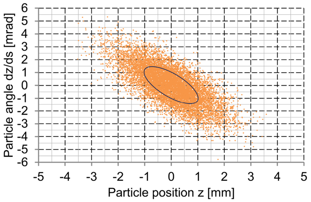
Figure 2.
A cross-section of the gantry beamline through its bending midplane. The beam enters the gantry from the left. DDS stands for the dose delivery system. The isocenter represents the virtual crossing point of the outcoming and (prolonged) incoming beam axes.
Figure 2.
A cross-section of the gantry beamline through its bending midplane. The beam enters the gantry from the left. DDS stands for the dose delivery system. The isocenter represents the virtual crossing point of the outcoming and (prolonged) incoming beam axes.
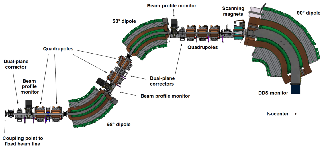
Figure 3.
An illustration of the fixed beamline matching-role and beam preparation at the beamline exit. Vertical plane: π mm mrad, the blue emittance diagram. Horizontal plane: π mm mrad (the bar-thin ellipse). The red emittance diagram – mode I, the yellow emittance diagram – mode II, the light-green emittance diagram – mode III, positive , the dark-green emittance diagram – mode III, negative . All particle distributions are cut at 1rms.
Figure 3.
An illustration of the fixed beamline matching-role and beam preparation at the beamline exit. Vertical plane: π mm mrad, the blue emittance diagram. Horizontal plane: π mm mrad (the bar-thin ellipse). The red emittance diagram – mode I, the yellow emittance diagram – mode II, the light-green emittance diagram – mode III, positive , the dark-green emittance diagram – mode III, negative . All particle distributions are cut at 1rms.
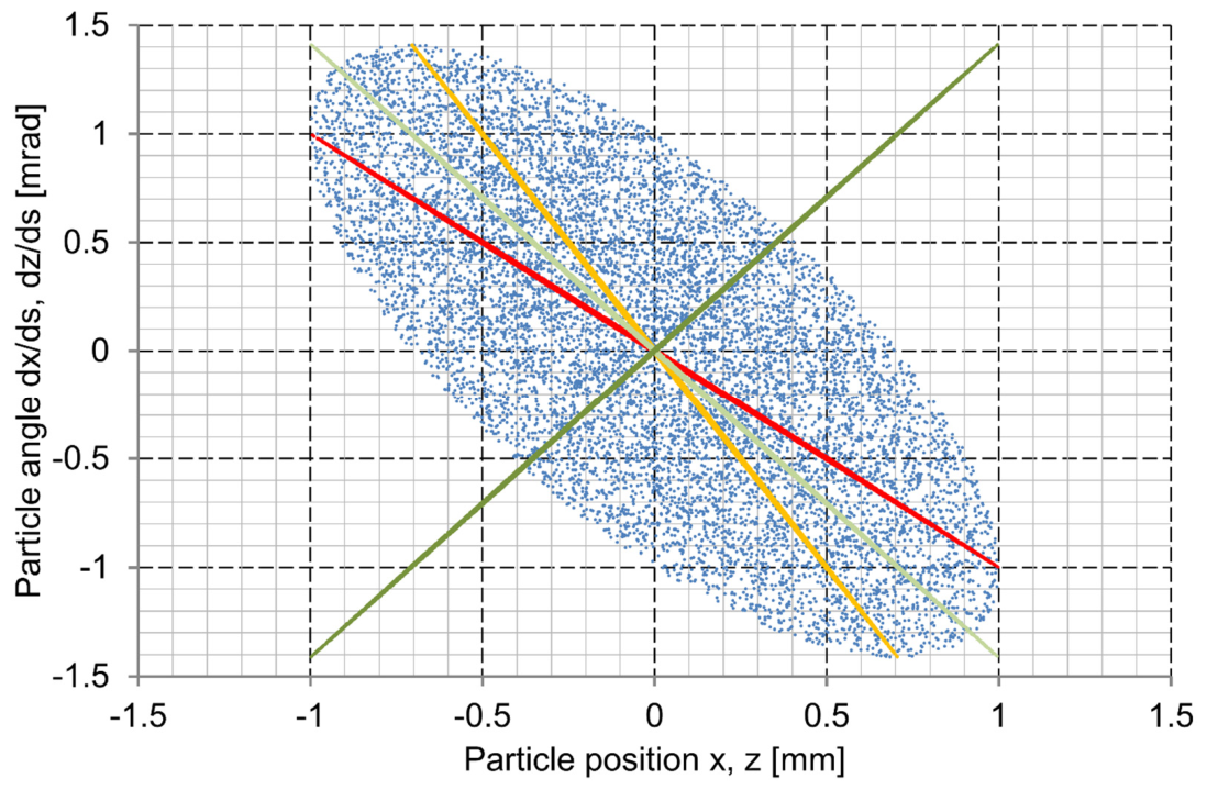
Figure 4.
Quadrupole excitations as a function of gantry magnification; the point-to-point rotatorlike imaging mode.
Figure 4.
Quadrupole excitations as a function of gantry magnification; the point-to-point rotatorlike imaging mode.
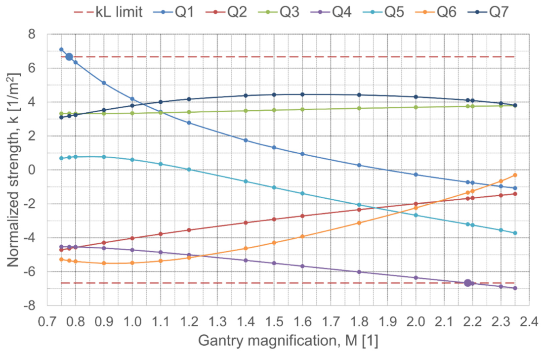
Figure 5.
FWHM (2.3548rms beam half-width) beam envelopes in the point-to-point rotatorlike gantry for the magnification . Red envelopes: gantry angle 90°. Blue envelopes: gantry angle 0°. Solid lines: full ellipse, dashed lines: bar-thin ellipse. Vertical solid lines: position of the gantry dipoles. Vertical dashed lines: position of the gantry quadrupoles (Q) and scanning magnets (S). DDS: the dose delivery system. Thick black lines: vacuum chamber aperture. Upper half of the plot: the vertical gantry plane, lower half of the plot: the horizontal gantry plane.
Figure 5.
FWHM (2.3548rms beam half-width) beam envelopes in the point-to-point rotatorlike gantry for the magnification . Red envelopes: gantry angle 90°. Blue envelopes: gantry angle 0°. Solid lines: full ellipse, dashed lines: bar-thin ellipse. Vertical solid lines: position of the gantry dipoles. Vertical dashed lines: position of the gantry quadrupoles (Q) and scanning magnets (S). DDS: the dose delivery system. Thick black lines: vacuum chamber aperture. Upper half of the plot: the vertical gantry plane, lower half of the plot: the horizontal gantry plane.
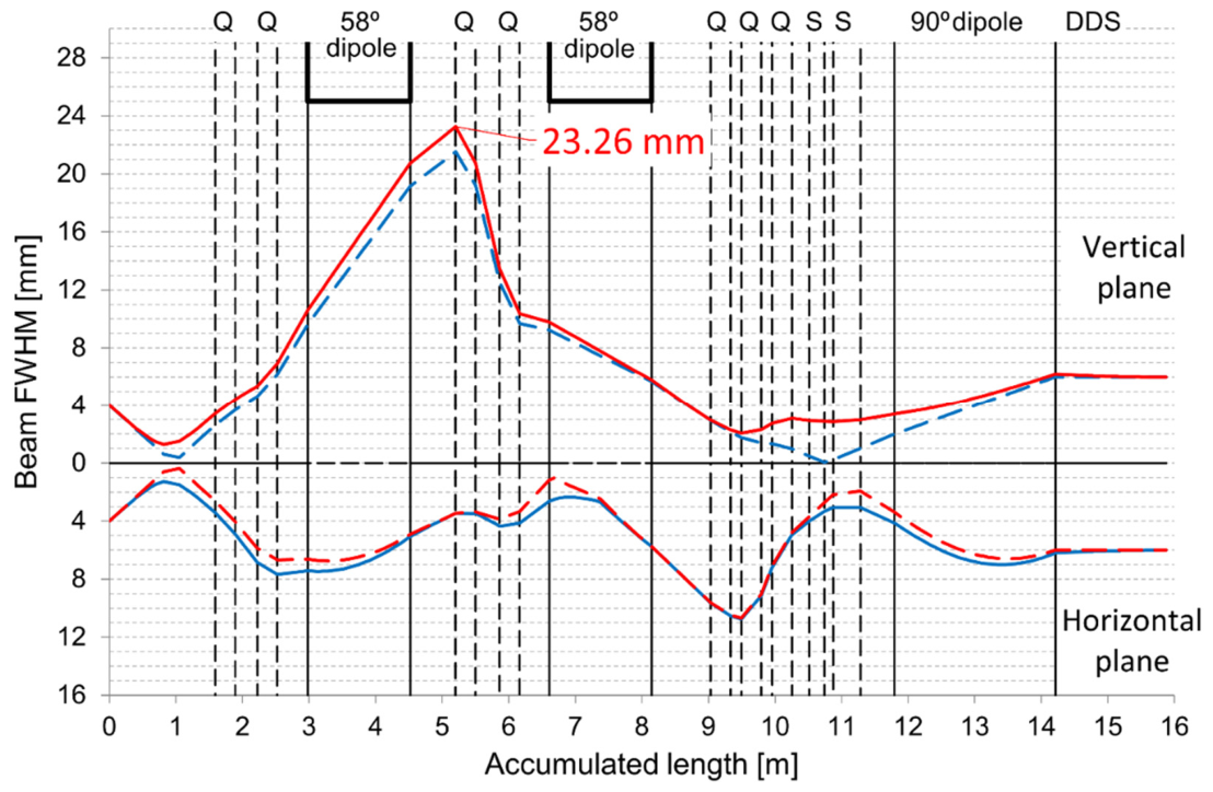
Figure 6.
Emittance diagrams at the HEBT exit (upper row) and the gantry isocenter (lower row). Blue diagrams: the full ellipse. Red diagrams: the bar-thin ellipse. Gantry magnification 1.5. The corresponding beam envelopes are shown in Figure 5.
Figure 6.
Emittance diagrams at the HEBT exit (upper row) and the gantry isocenter (lower row). Blue diagrams: the full ellipse. Red diagrams: the bar-thin ellipse. Gantry magnification 1.5. The corresponding beam envelopes are shown in Figure 5.
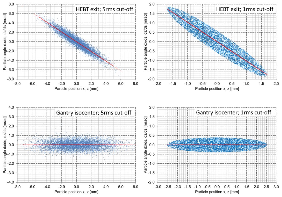
Figure 7.
Full-ellipse input Twiss parameters at the gantry entrance (left scale) and maximum beam-size inside the point-to-point rotatorlike gantry (the right scale) as a function of the gantry magnification. The large circles indicate where the technological limit of the quadrupoles is exceeded.
Figure 7.
Full-ellipse input Twiss parameters at the gantry entrance (left scale) and maximum beam-size inside the point-to-point rotatorlike gantry (the right scale) as a function of the gantry magnification. The large circles indicate where the technological limit of the quadrupoles is exceeded.
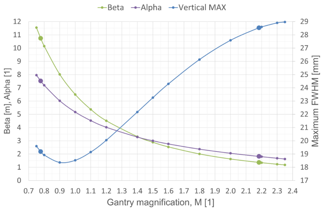
Figure 8.
Quadrupole excitations as a function of gantry magnification; the parallel-to-point rotatorlike imaging mode.
Figure 8.
Quadrupole excitations as a function of gantry magnification; the parallel-to-point rotatorlike imaging mode.
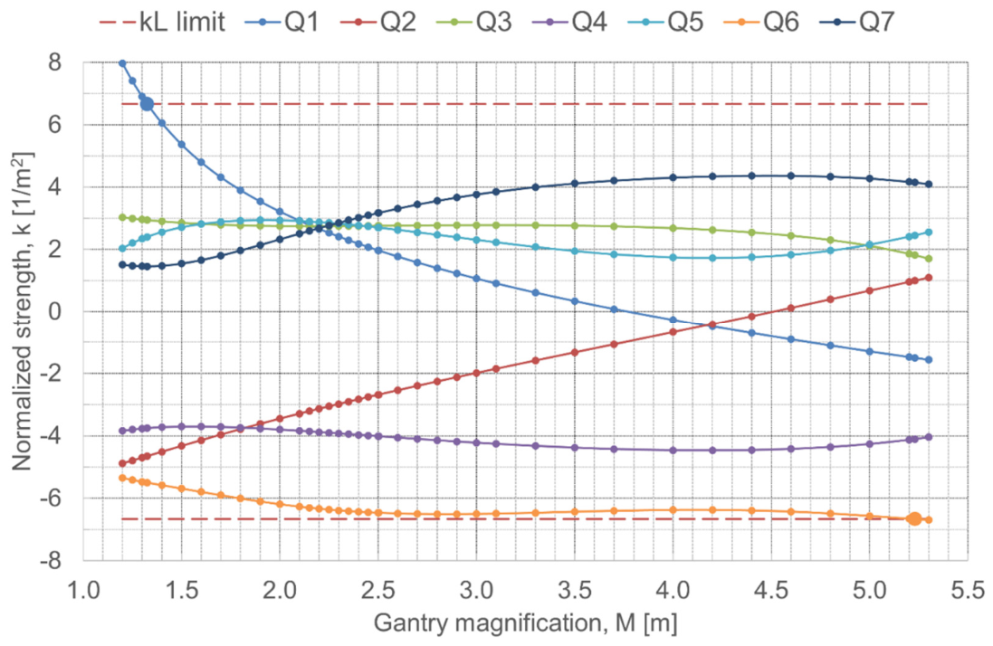
Figure 9.
FWHM (2.3548rms beam half-width) beam envelopes in the parallel-to-point rotatorlike gantry for the magnification m. Red envelopes: gantry angle 90°. Blue envelopes: gantry angle 0°. Solid lines: full ellipse, dashed lines: bar-thin ellipse. Vertical solid lines: position of the gantry dipoles. Vertical dashed lines: position of the gantry quadrupoles (Q) and scanning magnets (S). DDS: the dose delivery system. Upper half of the plot: the vertical gantry plane, lower half of the plot: the horizontal gantry plane.
Figure 9.
FWHM (2.3548rms beam half-width) beam envelopes in the parallel-to-point rotatorlike gantry for the magnification m. Red envelopes: gantry angle 90°. Blue envelopes: gantry angle 0°. Solid lines: full ellipse, dashed lines: bar-thin ellipse. Vertical solid lines: position of the gantry dipoles. Vertical dashed lines: position of the gantry quadrupoles (Q) and scanning magnets (S). DDS: the dose delivery system. Upper half of the plot: the vertical gantry plane, lower half of the plot: the horizontal gantry plane.
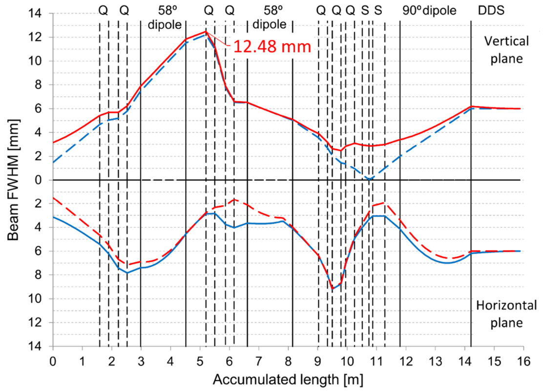
Figure 10.
Emittance diagrams at the HEBT exit (upper row) and the gantry isocenter (lower row). Blue diagrams: the full ellipse. Red diagrams: the bar-thin ellipse. Gantry magnification 3.0 m. The corresponding beam envelopes are shown in Figure 9.
Figure 10.
Emittance diagrams at the HEBT exit (upper row) and the gantry isocenter (lower row). Blue diagrams: the full ellipse. Red diagrams: the bar-thin ellipse. Gantry magnification 3.0 m. The corresponding beam envelopes are shown in Figure 9.
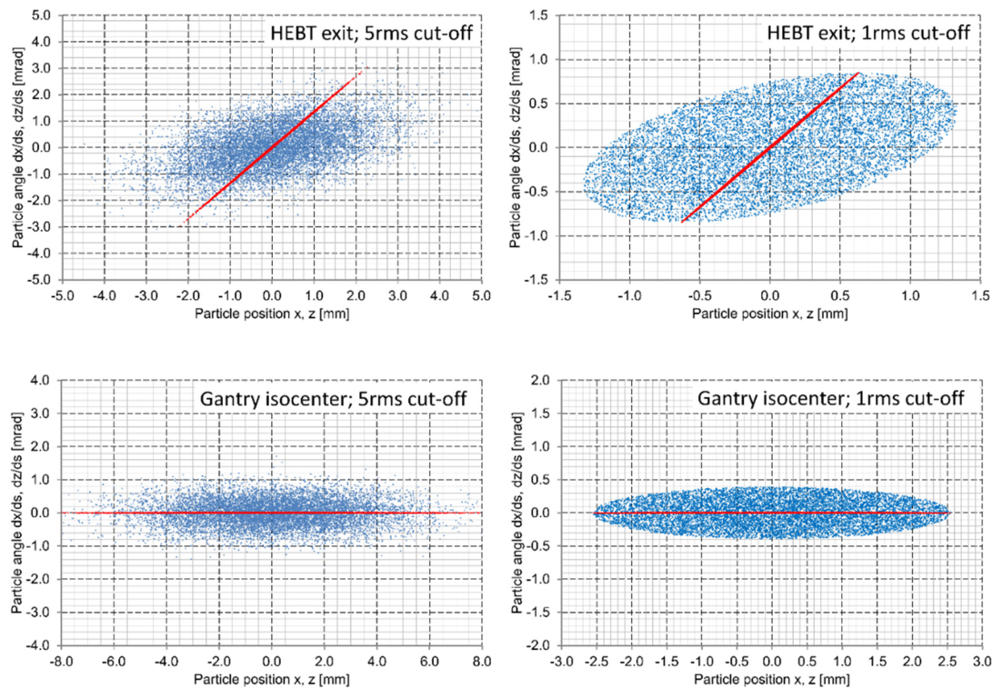
Figure 11.
Full-ellipse input Twiss parameters at the gantry entrance (left scale) and maximum beam-size inside the parallel-to-point rotatorlike gantry (the right scale) as a function of the gantry magnification. The large circles indicate where the technological limit of the quadrupoles is exceeded.
Figure 11.
Full-ellipse input Twiss parameters at the gantry entrance (left scale) and maximum beam-size inside the parallel-to-point rotatorlike gantry (the right scale) as a function of the gantry magnification. The large circles indicate where the technological limit of the quadrupoles is exceeded.
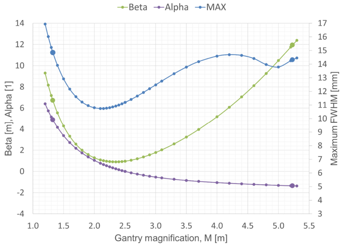
Figure 12.
FWHM (2.3548rms beam half-width) beam envelopes in the parallel-to-point rotatorlike gantry for the magnification m corresponding to the waist-to-waist beam-transport mode. Red envelopes: gantry angle 90°. Blue envelopes: gantry angle 0°. Black envelopes: present setting with the gantry magnification m. Solid lines: full ellipse, dashed lines: bar-thin ellipse. Vertical solid lines: position of the gantry dipoles. Vertical dashed lines: position of the gantry quadrupoles (Q) and scanning magnets (S). DDS: the dose delivery system. Upper half of the plot: the vertical gantry plane, lower half of the plot: the horizontal gantry plane.
Figure 12.
FWHM (2.3548rms beam half-width) beam envelopes in the parallel-to-point rotatorlike gantry for the magnification m corresponding to the waist-to-waist beam-transport mode. Red envelopes: gantry angle 90°. Blue envelopes: gantry angle 0°. Black envelopes: present setting with the gantry magnification m. Solid lines: full ellipse, dashed lines: bar-thin ellipse. Vertical solid lines: position of the gantry dipoles. Vertical dashed lines: position of the gantry quadrupoles (Q) and scanning magnets (S). DDS: the dose delivery system. Upper half of the plot: the vertical gantry plane, lower half of the plot: the horizontal gantry plane.
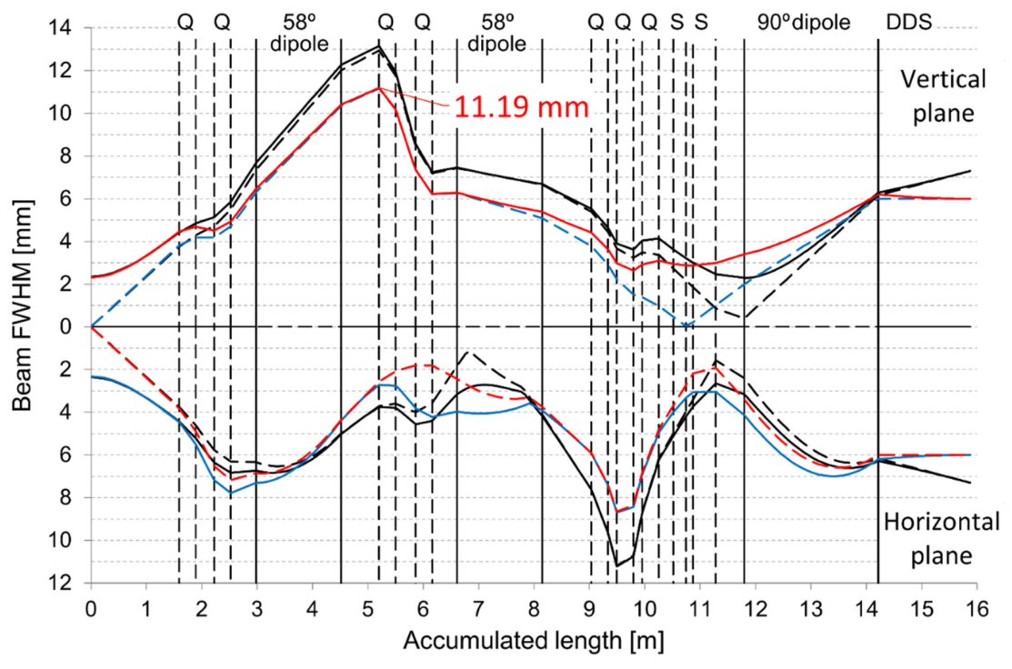
Figure 13.
FWHM (2.3548rms beam half-width) beam envelopes in the parallel-to-point rotatorlike gantry for the magnification m corresponding to the waist-to-waist beam-transport mode and . Red envelopes: gantry angle 90°. Blue envelopes: gantry angle 0°. Solid lines: full ellipse, dashed lines: bar-thin ellipse. Vertical solid lines: position of the gantry dipoles. Vertical dashed lines: position of the gantry quadrupoles (Q) and scanning magnets (S). DDS: the dose delivery system. Upper half of the plot: the vertical gantry plane, lower half of the plot: the horizontal gantry plane.
Figure 13.
FWHM (2.3548rms beam half-width) beam envelopes in the parallel-to-point rotatorlike gantry for the magnification m corresponding to the waist-to-waist beam-transport mode and . Red envelopes: gantry angle 90°. Blue envelopes: gantry angle 0°. Solid lines: full ellipse, dashed lines: bar-thin ellipse. Vertical solid lines: position of the gantry dipoles. Vertical dashed lines: position of the gantry quadrupoles (Q) and scanning magnets (S). DDS: the dose delivery system. Upper half of the plot: the vertical gantry plane, lower half of the plot: the horizontal gantry plane.
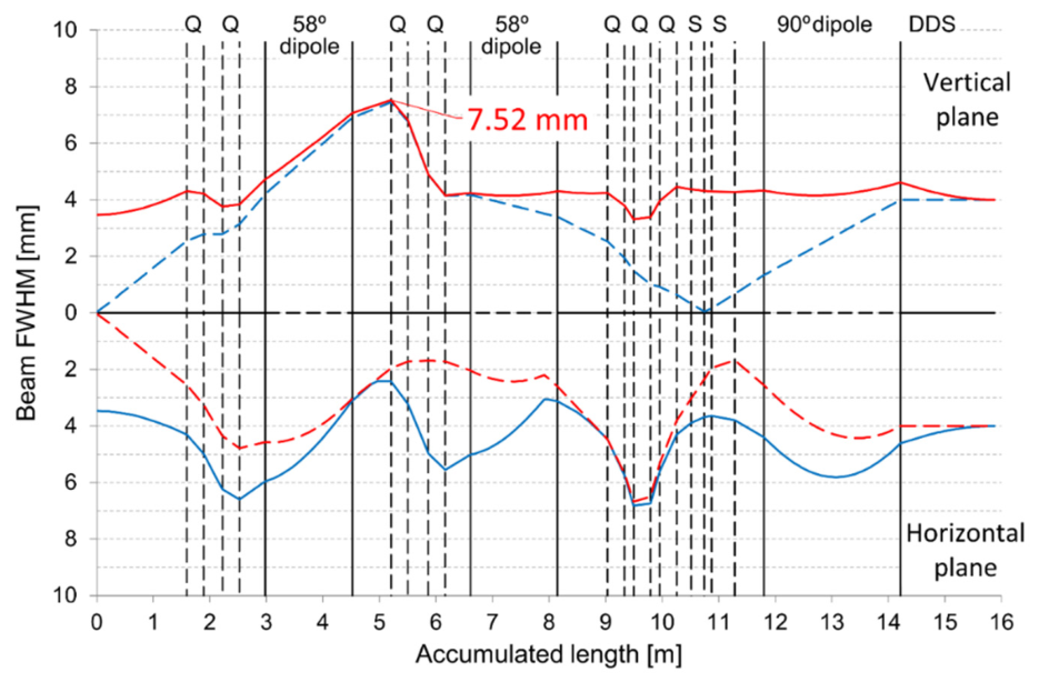
Figure 14.
Horizontal dispersion function. Red: point-to-point rotatorlike gantry. Black: parallel-to-point rotatorlike gantry. Vertical solid lines: position of the gantry dipoles. Vertical dashed lines: position of the gantry quadrupoles (Q) and scanning magnets (S). DDS: the dose delivery system.
Figure 14.
Horizontal dispersion function. Red: point-to-point rotatorlike gantry. Black: parallel-to-point rotatorlike gantry. Vertical solid lines: position of the gantry dipoles. Vertical dashed lines: position of the gantry quadrupoles (Q) and scanning magnets (S). DDS: the dose delivery system.
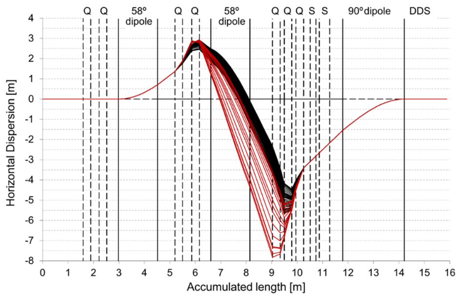

Table 1.
The configuration and main parameters of the beam transport system of the MedAustron proton gantry. The length of an element is its effective length used in beam transport calculations. The length of a dipole is the arc-length of the design orbit inside the dipole. The strength of a magnet is defined as the magnetic field gradient normalized to the magnetic beam-rigidity. Positive strength stands for vertical focusing (the WinAGILE sign convention). SFX stands for a scintillating fiber hodoscope beam-profile monitor. VW denotes a vacuum window, ITS means an independent termination system and intensity monitor, and DDS denotes a dose delivery system monitor. The quadrupole strengths correspond to the parallel-to-point imaging mode with gantry magnification of 3.1 m.
Table 1.
The configuration and main parameters of the beam transport system of the MedAustron proton gantry. The length of an element is its effective length used in beam transport calculations. The length of a dipole is the arc-length of the design orbit inside the dipole. The strength of a magnet is defined as the magnetic field gradient normalized to the magnetic beam-rigidity. Positive strength stands for vertical focusing (the WinAGILE sign convention). SFX stands for a scintillating fiber hodoscope beam-profile monitor. VW denotes a vacuum window, ITS means an independent termination system and intensity monitor, and DDS denotes a dose delivery system monitor. The quadrupole strengths correspond to the parallel-to-point imaging mode with gantry magnification of 3.1 m.
| Element | Length [m] | Strength [m-2] | More parameters and/or contained equipment | ||
|---|---|---|---|---|---|
| Drift | 1.593 | … | Dual-plane orbit corrector, SFX | ||
| Quadrupole 1 | 0.300 | 0.905 | Pole-to-pole aperture: 70 mm | ||
| Drift | 0.330 | … | … | ||
| Quadrupole 2 | 0.300 | –1.858 | Pole-to-pole aperture: 70 mm | ||
| Drift | 0.458 | … | … | ||
| 58° dipole | 1.538 | 0 | Entrance edge: +12°, exit edge: +12° | ||
| Drift | 0.683 | … | SFX | ||
| Quadrupole 3 | 0.300 | 2.777 | Pole-to-pole aperture: 70 mm | ||
| Drift | 0.360 | … | Dual-plane orbit corrector | ||
| Quadrupole 4 | 0.300 | –4.260 | Pole-to-pole aperture: 70 mm | ||
| Drift | 0.446 | … | … | ||
| 58° dipole | 1.538 | 0 | Entrance edge: +12°, exit edge: +12° | ||
| Drift | 0.888 | … | SFX, dual-plane orbit corrector | ||
| Quadrupole 5 | 0.300 | 2.228 | Pole-to-pole aperture: 70 mm | ||
| Drift | 0.160 | … | … | ||
| Quadrupole 6 | 0.300 | –6.494 | Pole-to-pole aperture: 70 mm | ||
| Drift | 0.160 | … | … | ||
| Quadrupole 7 | 0.300 | 3.850 | Pole-to-pole aperture: 70 mm | ||
| Drift | 1.541 | … | Vertical and horizontal scanning magnets | ||
| 90° dipole | 2.419 | 0 | Entrance edge: +11.9°, exit edge: +23° | ||
| Drift | 1.660 | … | Gantry nozzle (VW, ITS, DDS) | ||
| Isocenter | … | … | Scanning field 20 cm × 12 cm (Hor. × Vert.) | ||
Table 2.
The matching role of the incoming fixed beamline and definition of three possible modes of beam preparation at the fixed beamline exit.
Table 2.
The matching role of the incoming fixed beamline and definition of three possible modes of beam preparation at the fixed beamline exit.
| Mode I | Mode II | Mode III |
Table 3.
Sigma-matrix terms and the Twiss parameters at the fixed beamline exit corresponding to Figure 3. The numbers marked with * are rounded to three decimal places.
Table 3.
Sigma-matrix terms and the Twiss parameters at the fixed beamline exit corresponding to Figure 3. The numbers marked with * are rounded to three decimal places.
| Mode I | Mode II | Mode III | |
| Vertical plane of the fixed beamline, π mm mrad, the full ellipse | |||
| [m] | 1 | 1 | 1 |
| [mm2] | 1 | 1 | 1 |
| [1] | 1 | 1 | 1 |
| [mm⋅mrad] | –1 | –1 | –1 |
| [m-1] | 2 | 2 | 2 |
| [mrad2] | 2 | 2 | 2 |
| Horizontal plane of the fixed beamline, π mm mrad, the bar | |||
| [m] | 100 | 50.005 | 100 |
| [mm2] | 1 | 0.50005 | 1 |
| [1] | 100 | 100 | ±141.418* |
| [mm⋅mrad] | –1 | –1 | ±1.414* |
| [m-1] | 100.01 | 200 | 200 |
| [mrad2] | 1.0001 | 2 | 2 |
Disclaimer/Publisher’s Note: The statements, opinions and data contained in all publications are solely those of the individual author(s) and contributor(s) and not of MDPI and/or the editor(s). MDPI and/or the editor(s) disclaim responsibility for any injury to people or property resulting from any ideas, methods, instructions or products referred to in the content. |
© 2026 by the authors. Licensee MDPI, Basel, Switzerland. This article is an open access article distributed under the terms and conditions of the Creative Commons Attribution (CC BY) license (http://creativecommons.org/licenses/by/4.0/).
Copyright: This open access article is published under a Creative Commons CC BY 4.0 license, which permit the free download, distribution, and reuse, provided that the author and preprint are cited in any reuse.


