

Submitted:
05 July 2026
Posted:
06 July 2026
You are already at the latest version
Abstract
This paper proposes an optimal photovoltaic (PV) and battery storage system sizing procedure for a small-industrial building under uncertainty, using real high-resolution electricity consumption and PV production data. The techno-economic optimization framework considers discounted cash flow metrics such as Net Present Value (NPV), Internal Rate of Return (IRR), payback period, and annual energy savings to assess how different scenarios and combinations affect electricity cost and energy self-sufficiency. Focusing on a small-industrial scale case study under the net-billing scheme, it is demonstrated that larger PV systems can deliver substantial annual savings and investment value, especially when electricity prices are high and export compensation is low. Battery storage increases self-consumption and operational flexibility but maximizes NPV only when a substantial scale PV system is installed. Sensitivity analysis shows that optimal capacity choices are highly dependent on electricity price growth, discount rates, and export compensation. The results apply to firms, energy managers, and policy makers seeking to accelerate renewable adoption, enhance energy resilience, and improve their carbon footprint.
Keywords:
photovoltaic systems
; battery energy storage
; optimal sizing
; net billing
; self-consumption
; techno-economic analysis
1. Introduction
The transition toward renewable energy systems has become one of the central policy objectives of modern economies. Rising energy costs, climate change concerns, and the increasing need for energy security have accelerated investments in photovoltaic (PV) and battery energy storage systems (BESS). Industrial firms, in particular, are increasingly adopting renewable technologies to reduce electricity costs, improve sustainability performance, and hedge against volatility in electricity markets.
Despite the rapid decline in photovoltaic installation costs, optimal renewable energy investment decisions remain complex due to uncertainty regarding electricity prices, demand patterns, technology costs, and export compensation mechanisms. The intermittent nature of solar production also creates mismatches between energy generation and consumption. Battery storage systems can partially address these challenges by increasing self-consumption and reducing dependence on the electricity grid.
The existing literature has increasingly recognized the importance of managerial flexibility and investment timing in renewable energy projects. Real options frameworks and techno-economic optimization models have been used to study PV investments, storage adoption, and smart grid integration. For example, [1] develop a real options framework for PV-battery systems and show that battery storage increases investment flexibility and self-consumption. Similarly, [2] demonstrate that smart grid integration and peer-to-peer exchange can increase optimal investment size and investment value.
This paper builds on this literature by examining optimal PV and battery sizing using high-resolution industrial energy data. Unlike many existing studies focusing on residential systems, the small-industrial application case study in this work is characterized by relatively large-scale electricity consumption and detailed interval-level operational data. The analysis evaluates the economic performance of alternative PV and battery combinations under realistic tariff structures and investment assumptions.
The paper contributes to the literature in several ways. First, it provides a detailed techno-economic analysis using real industrial electricity demand and PV generation data. Second, it jointly evaluates PV expansion and battery storage decisions under a net-billing framework. Third, it examines how discount rates, electricity price growth, and export compensation influence optimal investment size and project profitability.
The remainder of the paper is organized as follows. Section 2 reviews the relevant literature. Section 3 presents the data and methodology employed in the analysis. Section 4 discusses the empirical results and sensitivity analysis. Finally, Section 6 concludes the paper and outlines directions for future research.
2. Related Literature
The literature on renewable energy investment has expanded significantly over the last decade. Existing studies have examined the economics of photovoltaic systems, battery storage technologies, self-consumption optimization, and smart grid integration.
A major strand of literature focuses on the valuation of PV systems coupled with storage. A real options framework for PV-battery systems was developed in [1], showing that battery storage increases investment flexibility and self-consumption. Their results show that battery adoption increases managerial flexibility and encourages larger PV investments. Similarly, smart-grid connected photovoltaic systems were investigated in [2], demonstrating that energy exchange between prosumers increases investment value and optimal plant size.
Several studies examine the economics of self-consumption and storage optimization. The literature on photovoltaic self-consumption in buildings was reviewed in [3], highlighting the importance of demand profiles and storage technologies. The optimal sizing of residential PV-battery systems was analysed in [4], showing that storage significantly increases self-consumption and profitability.
Another important strand focuses on techno-economic optimisation. Integrated optimisation of photovoltaic and battery systems for commercial buildings was investigated in [5]. The optimisation of self-consumption and self-sufficiency in commercial PV-battery systems was examined in [6] using real load and solar generation data from a supermarket in Germany.
Their findings show that while PV installations significantly reduce electricity costs and increase self-consumption, battery storage was not economically attractive under the 2015 cost assumptions, although future reductions in battery costs could improve feasibility.
Real options theory has also become increasingly important in renewable energy investment analysis. The foundational framework for investment under uncertainty was established in [7], while residential solar investments were analysed using a real options approach in [8].
The economics of battery storage have attracted growing attention as storage costs decline. Investment and risk appraisal in energy storage systems using real options methods was investigated in [9]. More recently, optimal investment in energy storage systems was examined in [10], showing that battery storage significantly increases operational flexibility but remains highly sensitive to energy prices and capital costs.
This paper contributes to the literature by focusing on industrial-scale renewable energy systems using detailed operational data and evaluating optimal capacity expansion under realistic market conditions.
3. Data and Methodology
The empirical analysis develops a detailed techno-economic optimization framework for evaluating photovoltaic (PV) and battery energy storage investments using high-resolution operational electricity data of a production facility in Cyprus. The methodology combines interval-level electricity balancing, battery dispatch simulation, and discounted cash flow valuation. The framework relies on real electricity demand and PV generation measurements taken every 5 minutes at a manufacturing facility, using the most recent three years of data from 2023 through 2025.
The model evaluates alternative PV and battery configurations by simulating electricity imports, exports, battery charging and discharging, electricity cost savings, and investment performance over the full project lifetime. The methodology explicitly captures the interaction between electricity demand, solar generation, and battery storage under a net-billing framework where exported electricity may receive lower compensation than imported electricity.
4. Model Formulation
4.1. PV Capacity Scaling
To evaluate PV systems of different sizes, a scaling factor k is introduced. This factor represents the ratio between a candidate PV system size and the existing reference PV installation.
The currently installed PV system has a rated capacity of
For this reference system, real PV production measurements are available. Electricity consumption and PV production data are recorded using a smart meter at 5-minute intervals.
For a candidate PV system characterized by the scaling factor k, the PV energy generated during time interval t is expressed as
where is the PV energy generated during interval t for the scaled system, is the measured energy production of the base PV system during interval t, and k is the PV scaling factor.
Equation (2) assumes that the electricity production profile scales proportionally with the installed PV capacity. Therefore, increasing k results in a proportional increase in PV energy generation while preserving the temporal characteristics of the measured production profile.
The total installed PV capacity corresponding to the scaling factor k is given by
where K denotes the installed PV capacity in kWp.
The scaling factor k is varied over a predefined range to investigate the sensitivity of electricity cost savings, investment profitability, and optimal system size with respect to photovoltaic capacity expansion.
4.2. Electricity Bills
The energy consumed during each 5-minute interval is in kWh. The effective import and export prices are and . In the current analysis we assume which corresponds to a net-billing scheme in which exported electricity is not remunerated, i.e., a zero-export configuration.
For each interval t, electricity imports and exports are computed as
where
- is electricity imported from the grid
- is electricity exported to the grid
Bill without PV:
In the absence of photovoltaic (PV) generation, the consumer must import the entirety of their electricity demand from the grid. The corresponding annual electricity expenditure is given by
where T denotes the set of time steps spanning the full year, is the electricity import price, and represents the load at time t.
Analogously, the electricity bill for a given month m is expressed as
where denotes the set of time steps corresponding to the billing interval of month m.
Bill with PV:
For a photovoltaic (PV) system with capacity scaling factor k, the total electricity expenditure is given by
where and denote, respectively, the imported and exported electricity at time step t, and and are the corresponding unit prices.
Analogously, the monthly electricity bill can be expressed as
where denotes the set of time steps belonging to month m.
If exported electricity does not yield any monetary compensation (i.e., if ), the export-related term vanishes from both expressions.
Electricity savings:
Savings from installing PV are defined as the reduction in electricity costs relative to the no-PV scenario.
Monthly savings are
Annual savings are
which can also be written as:
4.3. Project Valuation
Assuming annual savings grow at rate g, the present value of lifetime savings is
where r is the discount rate and T is project lifetime.
Net present value is therefore:
The payback period is
The internal rate of return solves
4.4. Optimal PV System Size
The model is evaluated for a range of PV scaling parameters k, selecting the one with the highest .
For each value of k, the interval imports, exports, electricity bills, and savings are computed. The resulting annual savings function where provides a measure of the economic benefit of installing larger PV systems.
Plotting against K allows us to identify the point at which is maximized.
4.5. Approximation of PV Installation Costs and Other Base Case Parameters
The PV installation cost per kWp is estimated using the logarithmic fit:
where K denotes installed PV capacity.
Total capital expenditure is therefore:

Table 1.
Estimated PV installation cost (CAPEX) by system size (for Cyprus)
| System size (kWp) | CAPEX (€) |
|---|---|
| 0 | 0 |
| 10 | 10,050 |
| 100 | 79,590 |
| 200 | 146,589 |
| 300 | 208,835 |
| 400 | 267,995 |
To evaluate the Net Present Value () of the project we assume a discount rate equal to which is in line with what is recommended in [11]. We assume that and that . In the baseline analysis, we adopt a conservative specification in which the growth rate of annual savings is assumed to be zero, i.e., and . For the determination of annual savings in the financial evaluation, the mean value of savings observed over the preceding three years is applied.
Table 2 shows the financial evaluation of each of the above alternative assuming a present value of savings over a horizon of years . Importantly, all alternative scenarios offer a quick payback, positive NPV and high IRR.
In Figure 1, the sensitivity of the results with respect to the installed capacity of the photovoltaic (PV) system is illustrated.
The corresponding quantitative outcomes, reported in Table 2, indicate that the optimal PV size is 240 kWp, which yields an estimated average annual cost savings of €55,533, a payback period of 3.1 years, a net present value over a 20-year operational horizon (net of installation costs) of €520,127 and a rate of return of more than 32%.
4.6. Sensitivity Analysis to Electricity Price Growth and Risk
Table 3 reports the optimal PV system size under alternative assumptions. Under the baseline parameters the optimal system size is 240 kWp, generating an NPV of €520,127 and an IRR of 32.18%. Under rising prices, annual cost savings are expected to increase. To capture this effect, the analysis is repeated under the assumption that electricity prices, and consequently the associated savings, grow at a conservative rate of 2% per annum. Under this scenario, the results indicate that the optimal system size increases to 270 kWp and that the project’s net present value (NPV) rises substantially.
In contrast, when a higher discount rate of 8% is applied, to reflect elevated investment risk, the optimal system size decreases to 210 kWp and the corresponding NPV is reduced.
5. Battery Optimization and Choice of Hybrid PV
We extend the baseline PV investment problem by allowing the decision maker to jointly determine the optimal PV system size and battery capacity. The objective is to identify the combination that maximises project value under the observed 5-minute electricity consumption and PV production profiles.
5.1. Decision Variables
The optimisation problem involves two decision variables:
- : PV system scale in kWp,
- : battery capacity in kWh.
For each candidate pair , the model simulates the energy flows, computes electricity savings, and evaluates the financial performance of the project.
5.2. Battery Storage Dynamics
The battery operation is modelled using a rule-based dispatch algorithm applied at the five-minute interval level. In each period, photovoltaic (PV) generation first serves on-site electricity demand. When PV production exceeds consumption, the surplus energy is used to charge the battery subject to battery capacity limits, charging power limits, and charging efficiency.
If electricity demand exceeds PV production, the battery discharges to cover the deficit before electricity is imported from the grid. The amount of energy discharged is limited by the available state of charge, the discharging power constraint, and the battery discharging efficiency. The state of charge of the battery evolves dynamically over time according to the charging and discharging flows while remaining bounded between zero and the maximum battery capacity.
This operational rule prioritizes self-consumption of PV generation and allows the battery to store excess daytime production for later use during periods of higher electricity demand. As a result, battery storage increases the share of PV energy consumed on-site and reduces reliance on grid electricity.
Let denote the battery state of charge at the end of interval t, measured in Wh. Battery capacity in Wh is
The state of charge is bounded by
Let and denote maximum charging and discharging power in kW. The corresponding 5-minute energy limits are presented in Equation 21 and 22.
Charging and discharging efficiencies are denoted by
5.3. Energy Dispatch
PV generation is first used to serve contemporaneous load demand. The residual deficit after PV generation is
while the PV surplus is
5.3.1. Battery Discharging:
When a deficit occurs, the battery discharges energy to support the load. The discharged energy is limited by the demand deficit, the available energy stored in the battery, and the maximum discharge rate
Grid imports are therefore
The state of charge evolves according to
where is the energy imported from the grid and is the battery state of charge at time interval t.
5.3.2. Battery Charging:
When PV generation exceeds load, the battery is charged using surplus PV energy. The charging energy is constrained by the available surplus energy, the remaining battery capacity, and the maximum charging rate
Exports to the grid are
The state of charge evolves as
where denotes the exported energy and is the energy charged into the battery during interval t.
5.4. Electricity Bills
Let and denote electricity import and export prices in euro per kWh. The electricity bill with PV and battery is calculated from the total imported and exported energy over the simulation period
The bill without PV is
Annual savings are therefore obtained as the difference between the electricity bill without PV and battery and the bill with PV and battery
5.5. Investment Costs
Total investment cost is given by
where represents the installation cost of the PV system (estimated as previously described), and corresponds to the installation cost of the battery.
Battery cost is approximated as
where is a fixed installation cost, is the cost per kWh of battery capacity, and is the cost per kW of charging power. We have used and based on current market estimates of battery costs.
5.6. Joint Optimization
The optimal PV and battery configuration is obtained by maximising the net present value of the investment
In the empirical implementation, this optimisation is performed by evaluating a grid of candidate PV sizes and battery capacities. For each pair , the model simulates battery operation over the full 5-minute dataset, computes annual electricity savings, and evaluates the financial metrics of the project.
The PV-only benchmark is obtained by setting
In this case, all PV surplus is exported to the grid and all residual electricity demand is satisfied through grid imports.
5.7. Hybrid PV and Battery Size Optimization Results
Table 4 reports the optimal PV and battery capacity combinations for different levels of available investment capital.
Several patterns emerge from the numerical analysis. First, at relatively low investment levels (below approximately €125,000), the optimal solution consists of installing PV capacity only without battery storage. In this region battery investments are not cost-effective because the marginal value of additional PV self-consumption remains limited.
Second, as investment budgets increase beyond €150,000, battery storage becomes economically attractive. At these higher investment levels the optimal strategy involves jointly expanding PV capacity and battery storage. Batteries allow excess daytime PV generation to be stored and used later during periods of higher electricity demand, thereby increasing overall self-consumption and reducing grid imports.
Third, while larger investment budgets increase the absolute level of NPV, the marginal return to investment declines. This is reflected in the gradual decrease in internal rates of return from approximately 46% for small PV systems to around 24% for the largest PV–battery combinations considered. Similarly, payback periods increase as larger system sizes are installed.
Overall, the numerical results indicate that PV installations generate strong economic value under current electricity prices in Cyprus, and battery storage becomes attractive once PV capacity reaches sufficiently large levels. The optimal investment frontier therefore involves initially expanding PV capacity followed by the gradual addition of battery storage as investment budgets increase.
6. Conclusion
This paper examined the optimal sizing of photovoltaic and battery storage systems using high-resolution industrial load data. The analysis combined techno-economic optimization with discounted cash flow valuation methods to evaluate the economic performance of alternative renewable energy investments.
The results show that large-scale photovoltaic expansion can generate substantial economic benefits through electricity cost savings and increased self-consumption. Battery storage increases operational flexibility and reduces dependence on grid electricity, although its economic attractiveness becomes significant when combined with large PV systems.
Sensitivity analysis demonstrated that electricity price growth and discount rates critically influence optimal system size and investment profitability. Overall, the findings support continued renewable energy investment in industrial applications and highlight the importance of policy frameworks that encourage self-consumption and storage adoption.
Future research could extend the analysis by incorporating stochastic electricity prices, dynamic battery degradation, real options valuation, and demand response interactions.
Acknowledgments
This research has received support from the project EP/CETP/0923/0010 (CoEnerBuild), implemented under the Cohesion Policy Funds “THALIA 2021–2027” of the Republic of Cyprus with co-funding by the European Union. The authors would also like to acknowledge the valuable collaboration and support of A.P. Georgiades Ltd in facilitating the collection and analysis of real operational energy data used in this study.
References
- Andreolli, F.; D’Alpaos, C.; Moretto, M. Valuing investments in domestic PV-Battery Systems under uncertainty. Energy Econ. 2022, 106, 105721. [Google Scholar] [CrossRef]
- Castellini, M.; Menoncin, F.; Moretto, M.; Vergalli, S. Photovoltaic Smart Grids in the prosumers investment decisions: a real option model. J. Econ. Dyn. Control 2021, 126, 103988. [Google Scholar] [CrossRef]
- Luthander, R.; Widén, J.; Nilsson, D.; Palm, J. Photovoltaic self-consumption in buildings: A review. Appl. Energy 2015, 142, 80–94. [Google Scholar] [CrossRef]
- Weniger, J.; Tjaden, T.; Quaschning, V. Sizing of residential PV battery systems. Energy Procedia 2014, 46, 78–87. [Google Scholar] [CrossRef]
- Mariaud, A.; Acha, S.; Ekins-Daukes, N.; Shah, N.; Markides, C.N. Integrated optimisation of photovoltaic and battery storage systems for UK commercial buildings. Appl. Energy 2017, 199, 466–478. [Google Scholar] [CrossRef]
- Merei, G.; Moshövel, J.; Magnor, D.; Sauer, D.U. Optimization of self-consumption and techno-economic analysis of PV-battery systems in commercial applications. Appl. Energy 2016, 168, 171–178. [Google Scholar]
- Dixit, A.K.; Pindyck, R.S. Investment under uncertainty; Princeton university press, 1994. [Google Scholar]
- Vargas, C.; Chesney, M. What are You Waiting to Invest? Long-Term Investment in Grid-Connected Residential Solar Energy in California. A Real Options Analysis. Long-Term Investment in Grid-Connected Residential Solar Energy in California. A Real Options Analysis.(May 24, 2019) 2019.
- Locatelli, G.; Invernizzi, D.C.; Mancini, M. Investment and risk appraisal in energy storage systems: A real options approach. Energy 2016, 104, 114–131. [Google Scholar] [CrossRef]
- Castellini, M.; D’Alpaos, C.; Fontini, F.; Moretto, M. Optimal investment in an energy storage system. Eur. J. Oper. Res. 2025. [Google Scholar] [CrossRef]
- European Commission. Economic Appraisal Vademecum 2021–2027: General Principles and Sector Applications. Technical report, Directorate-General for Regional and Urban Policy, Brussels, Belgium, 2021. Inforegio publication. [CrossRef]
Figure 1.
Optimal PV choice without batteries: base case. Notes: The figure illustrates the sensitivity of the system size and the corresponding impact on the project’s net present value (NPV).
Figure 1.
Optimal PV choice without batteries: base case. Notes: The figure illustrates the sensitivity of the system size and the corresponding impact on the project’s net present value (NPV).
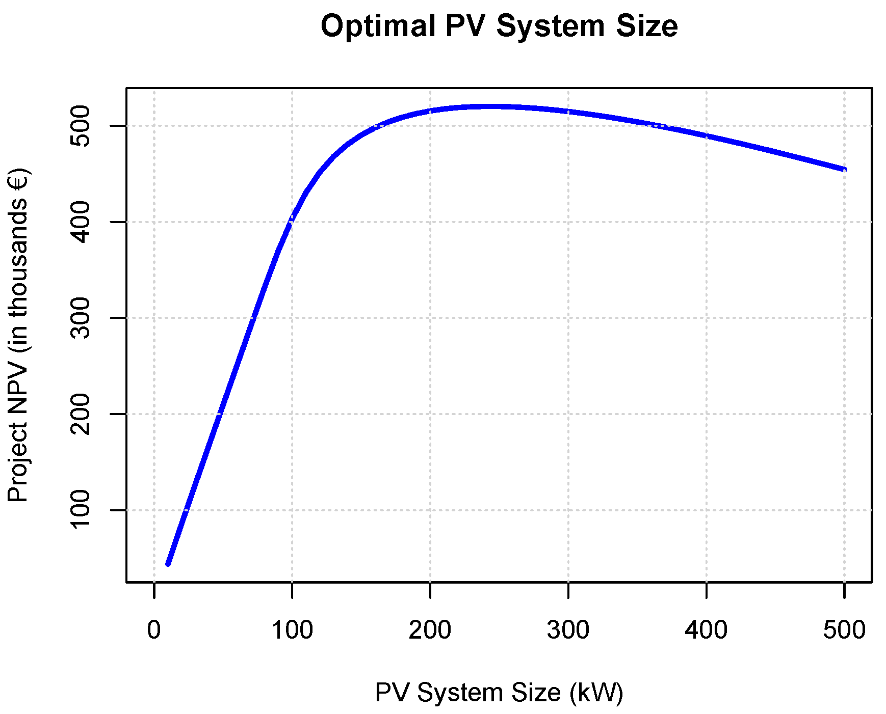
Table 2.
Financial performance of PV investments
| System (kWp) | CAPEX (€) | Payback (yrs) | NPV (€) | IRR |
|---|---|---|---|---|
| 10 | 10,050 | 2.32 | 43,920 | 43.05% |
| 50 | 42,943 | 2.12 | 209,748 | 47.20% |
| 70 | 57,981 | 2.07 | 291,506 | 48.35% |
| 100 | 79,590 | 2.05 | 403,533 | 48.69% |
| 150 | 113,861 | 2.35 | 490,293 | 42.54% |
| 200 | 146,589 | 2.76 | 515,459 | 36.17% |
| 240 | 171,932 | 3.10 | 520,127 | 32.18% |
| 250 | 178,169 | 3.18 | 520,064 | 31.31% |
| 300 | 208,835 | 3.60 | 514,846 | 27.59% |
| 400 | 267,995 | 4.41 | 489,521 | 22.27% |
Table 3.
Sensitivity analysis of optimal PV system size
| Case | Sys | 2025 | 2024 | 2023 | Avg | CAPEX | NPV | IRR |
|---|---|---|---|---|---|---|---|---|
| Base case | 240 | 52,265 | 51,424 | 62,909 | 55,533 | 171,932 | 520,127 | 32.18% |
| Higher growth () | 270 | 53,476 | 52,703 | 64,588 | 56,922 | 190,535 | 644,255 | 31.70% |
| Higher risk () | 210 | 50,724 | 49,862 | 60,825 | 53,804 | 152,988 | 375,264 | 35.08% |
Table 4.
Optimal PV and battery size under CAPEX constraints
| Limit | PV | Batt. | Savings | Payback | NPV | IRR |
|---|---|---|---|---|---|---|
| (€) | (kWp) | (kWh) | (€/yr) | (yrs) | (€) | (%) |
| 25k | 20 | 0 | 8,122 | 2.32 | 82,376 | 43.1 |
| 50k | 50 | 0 | 19,130 | 2.24 | 195,456 | 44.5 |
| 75k | 90 | 0 | 33,323 | 2.18 | 342,780 | 45.9 |
| 100k | 120 | 0 | 41,221 | 2.27 | 420,181 | 44.0 |
| 125k | 160 | 0 | 46,861 | 2.57 | 463,473 | 38.8 |
| 150k | 160 | 75 | 52,885 | 2.81 | 510,296 | 35.5 |
| 175k | 180 | 100 | 56,842 | 2.98 | 538,730 | 33.4 |
| 200k | 200 | 150 | 61,919 | 3.20 | 573,555 | 31.1 |
| 225k | 210 | 200 | 65,715 | 3.35 | 598,965 | 29.7 |
| 250k | 230 | 250 | 70,508 | 3.52 | 630,533 | 28.2 |
| 275k | 260 | 275 | 74,594 | 3.68 | 654,985 | 26.9 |
| 300k | 260 | 350 | 78,796 | 3.78 | 684,107 | 26.2 |
| 325k | 290 | 375 | 82,822 | 3.91 | 708,128 | 25.3 |
| 350k | 320 | 400 | 86,299 | 4.05 | 725,600 | 24.3 |
| 375k | 340 | 400 | 87,385 | 4.14 | 727,197 | 23.8 |
Disclaimer/Publisher’s Note: The statements, opinions and data contained in all publications are solely those of the individual author(s) and contributor(s) and not of MDPI and/or the editor(s). MDPI and/or the editor(s) disclaim responsibility for any injury to people or property resulting from any ideas, methods, instructions or products referred to in the content. |
© 2026 by the authors. Licensee MDPI, Basel, Switzerland. This article is an open access article distributed under the terms and conditions of the Creative Commons Attribution (CC BY) license (http://creativecommons.org/licenses/by/4.0/).
Copyright: This open access article is published under a Creative Commons CC BY 4.0 license, which permit the free download, distribution, and reuse, provided that the author and preprint are cited in any reuse.


