

Submitted:
02 July 2026
Posted:
06 July 2026
You are already at the latest version
Abstract
Fatigue is widely recognized as one of the primary failure mechanisms affecting metallic structures. Consequently, reliable prediction of fatigue-induced failure is essential for the safe design and lifetime prediction of engineering structures and components. In this context, the present work provides an overview of some of the main approaches employed for fatigue modelling in metals. First, the classical total-life methods, namely the stress–life and strain–life approaches, are reviewed. Subsequently, fracture-based approaches to fatigue are presented, including formulations grounded in fracture mechanics, continuum damage mechanics, and phase-field theory. The finite element method and the extended finite element method are also discussed as representative numerical frameworks for the implementation of these formulations. The reviewed approaches are then critically compared, and their main characteristics are summarized in a comparative table. Finally, the principal features of the presented approaches are highlighted.
Keywords:
fatigue modeling
; total-life methods
; fracture mechanics
; continuum damage mechanics
; phase-field formulations
; fracture-based models
; finite element method
; extended finite element method
1. Introduction
Beginning in the mid-19th century, the study of fatigue in metals has become, over the years, a field of major interest for materials scientists and structural engineers, mainly because it represents one of the principal failure mechanisms in metallic engineering structures. Accordingly, early fatigue assessment was largely based on empirical approaches, notably the stress amplitude–life (S–N) curves derived from Wöhler’s pioneering studies [1,2,3] and the strain–life (–N) diagrams emerging from the works of Coffin [4] and Manson [5]. Commonly classified as total-life approaches, these methodologies were originally intended for fatigue life estimation and remain widely employed to predict the service life of metallic components. Since the emergence of these pioneering approaches, fatigue prediction capabilities have advanced considerably, culminating in the development of sophisticated numerical models capable of predicting not only fatigue life but also the progressive degradation of material properties associated with the fatigue damage, including crack initiation and propagation processes that ultimately lead to complete structural failure.
Approaches exhibiting these characteristics are commonly referred to as fracture-based fatigue models. Over the years, several classes of models encompassing such features have been developed. Their diversity and breadth make it impractical to provide a comprehensive treatment of all existing formulations within a single work. Nevertheless, since the introduction of the energy-based fracture theory proposed by Griffith in 1921 [6], three classes of models have gained sufficient relevance to deserve a comparative review, namely those grounded in frameworks of fracture mechanics [7,8] and continuum damage mechanics [9,10], and phase-field formulations [11,12]. Although originally developed to describe fracture under monotonic loading conditions, many formulations belonging to these classes have subsequently been extended to account for fatigue loading scenarios. Accordingly, in addition to the total-life approaches, this work presents a review of relevant fracture formulations within these classes of models and their extension to fatigue, followed by a general comparison among the presented approaches. Furthermore, the finite element method (FEM) and the extended finite element method (XFEM) are considered to frame the discussion from a numerical perspective, as they are among the most widely employed discretization strategies for modelling fracture and fatigue.
The remainder of this paper is organized as follows. Section 2 reviews the classical total-life approaches, namely the stress–life and strain–life methods. Section 3 presents fracture-based modelling approaches grounded in fracture mechanics, continuum damage mechanics, and phase-field formulations, together with their extensions to fatigue. A comparative assessment of the reviewed approaches is provided in Section 4 and their advantages and limitations are comparatively summarized in a table. Finally, Section 5 highlights the main features of each class of model discussed in this work.
2. Total-life Approaches
Total-life approaches constitute classical methods employed in fatigue analysis and design. With a focus on failure rather than the evolution of fatigue cracks, they are fundamentally characterized by life curves described in terms of cyclic stress or strain ranges, which correspond to the so-called stress- and strain-based methods, respectively. These curves are often obtained through standard fatigue tests conducted on polished coupon specimens under either constant amplitude stress- or strain-controlled regimes [13,14]. As a results, the number of cycles to nucleate and propagate a dominant crack until the specimen complete failure is measured. A general description of the main features of each method is presented in the following.
2.1. Stress-life Method
Grounded on the premise of global elastic response of the material under sub-critical stresses, the stress-life method has been traditionally applied in high-cycle fatigue (HCF) analysis, i.e., in cases in which the fatigue failure occurs after a high number of load cycles, often more than . This analysis is commonly performed using Wöhler curves obtained by the fitting of S-N experimental points. Accordingly, different approaches have been proposed to mathematically describe these curves [15,16]. Among them, the equation introduced by Basquin [17] has become particularly popular due to its simplicity. In the logarithmic form, it reads
where and represent the stress amplitude and number of cycle to failure, whereas C and m are model parameters fitted through the least square method. The stress amplitude, in turn, may be defined as
with and being the maximum and minimum stresses, respectively.
Figure 1 schematically illustrates the main features of typical S-N curves resulting from such a fitting procedure. As can be seen, these curves exhibit distinct patterns for ferrous and non-ferrous metallic material. In the case of ferrous alloys, they are often designed with a knee point followed by a plateau called fatigue limit. Beyond this point, a structure submitted to cyclic loads is assumed to withstand an infinite number of cycles, as far as the corresponding stress amplitude remains below this limit. In real applications, however, it is difficult to clearly define this knee point due to the scatter inherent to the fatigue phenomenon, as shown in the graphic by the range in which finite and infinite lives are overlapped. Despite that, it is a common practice to adopt values between and cycles for this point [18,19], avoiding – whenever possible – stress amplitudes close to the fatigue limit in infinite-life designs. Contrarily to ferrous metals, non-ferrous alloys do not exhibit a clear plateau, as illustrated in the graphic. Cutoff values are usually set for infinite-life designs though. For aluminum grades, for instance, values between and are typically assumed for this purpose [19,20].
S-N curves can be determined not only for coupon specimens but also for mechanical component and engineering structures in general. However, large-scale fatigue tests are extremely costly and, as a result, the use of specimen fatigue data – often assumed as material properties – obtained under controlled conditions is preferred whenever possible. Thus, when the design and life assessment of actual components are concerned, material S-N curves are modified in an attempt to adapt this specimen-level data to the part in-service conditions. This is commonly done by modifying the material nominal fatigue limit by the so-called Marin reduction factors to account for the influence of aspects such as surface condition, part size, load type, reliability, among others [21]. In its general form, the fatigue limit of the actual component is estimated through
where is the material nominal fatigue limit and , , , , , represent surface, size, loading, temperature, reliability and miscellaneous-effect factors.
In addition, the effect of stress concentrations induced by geometrical discontinuities such as grooves, holes and notches is also considered in this type of analysis. For this purpose, fatigue notch factors are applied to the nominal stress calculated using elasticity-based formulae to determine a "fatigue-effective" stresses [22,23], i.e.,
According to Peterson [23], for instance, this factor is given by
where is the classical stress concentration factor used in elasticity problems and q the so-called notch sensitivity. Typically depending on geometrical features, material properties and loading condition (e.g., axial, bending and torsional), q is defined between 0 and 1, assuming values close to the unity for large notch radius. Accordingly, in many practical cases, full notch sensitivity is assumed (i.e., and ) as a conservative measure, given the common scatter of the data used in the q estimation. In addition to the classical approaches, alternative methods such as those based on stress gradients [24], highly-stressed-volume [25] and theory of distances [26] have also been proposed to incorporate the notch effect in these fatigue analyses. Figure 2 schematically illustrates the notch effect on the stress field of an axially loaded notched specimen and how the stress concentration and notch factors are employed to estimate the peak and maximum stress, and , from the nominal counterpart, .
Standardized fatigue tests are typically conducted under a fully reversed load regime such that, the stress ratio
is equal to -1. In addition, a mean stress
equal to zero naturally follows from this load condition. However, load regimes leading to non-zero mean stresses are often found in real world applications. Since such mean stresses may have a significant influence in the material fatigue response, many different approaches have been proposed to account for their effects in fatigue analysis [27,28,29]. In practical terms, these approaches provide a way to calculate an equivalent stress amplitude at , given a stress amplitude and a mean stress at , which may be then confronted with the S-N data from fully reversed tests. Table 1 summarizes some of the most relevant mean stress correction models and their dependence on specific material parameters. Among them, the classical Geber [30], Goodman [31], Soderberg [33] and Morrow [34] models are also graphically shown in Figure 3.
Alternatively to the models presented in Table 1, Haigh [41] proposed an approach in which the mean stress correction is carried out according to four different stress ratio regimes (i.e., , , and ), as detailed in the FKM-Guideline [42].
Real fatigue load histories often exhibit varying amplitudes. Accordingly, numerous damage accumulation models have been proposed to handle the effect of cyclic load blocks of different stress amplitudes in fatigue calculations [43]. These models rely on damage parameters that cumulatively compute the contribution of each block to the overall material fatigue damage, acting ultimately as remaining life estimators. Among the existing models, the Palmgren-Miner linear accumulation rule
is widely used, mainly due to its simplicity [44,45]. Here is the number of cycles applied at a certain stress amplitude, , and the corresponding number of cycles to failure. D, in turn, represents the accumulated damage, which indicates failure when it reaches a critical value – typically equal to 1. Despite its wide practical use, this rule assumes that the damage accumulation is independent of the load block application order. As a consequence, it fails to capture non-linear load sequences and overload effects [46,47]. The appropriate use of damage accumulation rules require the adoption of an efficient cycle counting procedure, particularly for the cases of highly irregular load histories. Accordingly, the rain-flow method is the most widely used approach for this purpose [46]. It is based on the comparison of adjacent stress ranges such that a cycle is counted whenever the second range is greater than the first. Figure 4 shows an application example of the rain-flow counting procedure together with the corresponding percentage damage accumulated in each block of cyclic load.
The analytical solution of elasticity problems is usually limited to specific, idealized cases. For this reason, standard linear elastic finite element analyses (FEA) are commonly employed to computed the stress field, particularly when more complex geometries are involved. Hence, a stress norm such as von Mises is used to handle the multiaxial states arising from the FEA. Finally, the stress-life method is then applied as a post-processing operation to perform the fatigue analysis. The results from this type of analysis are usually represented either as a map of the number cycles to failure or the accumulated damage due to the application of predefined load blocks. In addition, a map of the safety factor, n, – conceptually obtained by substituting and by and in the equations of Table 1 – can also be plotted for design and verification purposes. Figure 5 illustrates the results of stress-life fatigue analyses carried out in conjunction with the linear elastic FEA.
2.2. Strain-life Method
In contrast to the stress-life approach, the strain-life method explicitly accounts for plasticity, providing as a result, a more robust foundation to handle fatigue problems in the low cycle domain – where macroscopic plastic strains become a relevant factor. As such, it constitutes a local approach in which the fatigue life – typically expressed by the number of reversals, , – is related to the total strain range, , through the well-known Coffin-Manson relationship [4,5], which is given by
where E is the material Young’s modulus, and are the fatigue strength and ductility coefficients and b and c the fatigue strength and ductility exponents. In addition, the first and second terms on the right side of this equation represent, respectively, the elastic and plastic strain ranges (i.e., and ). As an alternative to the classical Coffin-Manson approach, numerous strain-based methods have been proposed as fatigue life estimators. Examples include the modified universal slopes [51], uniform materials [52], Roessle-Fatemi’s hardness [53], modified Mitchell [54] and medians methods [55]. For a more comprehensive survey on them, the reader is referred to [56,57].
The fatigue constants of Equation (9) are usually determined by fitting experimental data from fully reversed strain-controlled fatigue tests. Stable stress-strain hysteresis loops – commonly recorded near the half of the specimen fatigue life – are employed for this purpose [58]. Figure 6 schematically represents a typical hysteresis loop used in this procedure, highlighting the stress range, , and the total, elastic, and plastic strain ranges – , and – associated with this type of curve.
The fatigue life estimation resulting from Equation (9) and the respective experimental data are usually represented in terms of the number of reversal, and the total strain amplitude, , as shown in Figure 7.
Despite the usual calibration through data from fully reversed tests, Equation (9) can be modified to account for the mean stress effect in fatigue analyses involving strain ratios, , different from -1. This can be done by correcting the number of cycles, , in this expression as follows
where can be any mean stress correction model depending on the stress amplitude and the mean stress such as those presented in Table 1 [58].
Analogous to the stress-life approach, damage accumulation rules and the rain-flow cycle counting procedure are commonly employed to handle variable amplitude load scenarios in fatigue analyses using the strain-life method. However, special care should be taken when analyzing highly irregular load histories in the low cycle regime, where plastic strains may play a critical role in the fatigue failure. This is particularly important because plasticity is a path-dependent phenomenon and Equation (9) assumes independent, stabilized cycles for the fatigue life estimation. Furthermore, an additional source of error may be introduced if the Palmgreen-Miner rule is adopted as the damage accumulation model, since it does not distinguish the sequence of the applied load blocks, as previously discussed. Consequently, the application of the strain-life method in these scenarios may lead to significant inaccuracies in fatigue life estimations.
As a local approach, the application of the strain-life method at the component level requires the determination of the total strain at the part critical locations – task that is hardly feasible through analytical solutions, particularly when dealing with intricate geometries. Thus, nonlinear FEA, incorporating a suitable plasticity material model (e.g., with isotropic or kinematic hardening), may be employed to obtain stable hysteresis stress-strain loops at the component critical points. These loops can then be used in a post-processing step to estimate the fatigue life through the Coffin-Manson relationship. For complex, lengthy load histories, however, plasticity models may lead to computationally highly expensive simulations, hampering their application in such scenarios. Alternatively, linear elastic FEA have been employed in conjunction with notch correction factors to estimate the elasto-plastic stresses and strains in the part hot spots [59,60].
3. Modeling Approaches for Fracture and Their Extension to Fatigue
Unlike the total-life methods, fracture models – when applied in the context of fatigue analysis – not only serve as life indicators but also provide a description of the crack growth process. Classical examples of them include the approaches based on the fracture mechanics (FM). Beyond modeling the crack propagation, some classes of fracture models – such as those grounded on the continuum damage mechanics (CDM) and phase-field (PF) method – are conceived to capture the entire degradation process, from the material intact condition up to its final failure. Since they three represent some of the most relevant classes of fracture model, a general overview of the principles underlying each of them is presented in the following.
3.1. Models Based on the Fracture Mechanics
Relying on the premise that engineering components are inherently flawed, classical fracture models formulated within the framework of the FM are often referred to as defect-tolerant approaches. Accordingly, these models focus on the growth of a pre-existing crack such that, in the context of fatigue, the corresponding life is defined as the number of cycles required to propagate this crack from its initial size up to a certain critical dimension.
Crack growth models within the framework of FM are generally classified into main categories: the linear elastic fracture mechanics (LEFM) and the elastic-plastic frature mechanics (EPFM). The primary distinction between them lies in the extent of the plastic zone ahead of the crack tip. In LEFM, this zone is assumed to be negligible, allowing linear elastic assumptions to hold. In contrast, EPFM accounts for significant plastic deformation in the crack-tip region.
Under the LEFM assumption, the stress singularity at the crack tip is handled by the scalar-valued intensity factor,
where represents the nominal stress and a the crack size, whereas is a dimensionless correction factor depending on the component geometry, size, shape of the crack and loading type. Polynomials and curves defining for basic configurations can be found in various handbooks [62,63,64,65].
The expression in Equation (11) serves as a general formulation, but it is important to note that crack propagation can occur in three fundamental modes, or a combination of them (see Figure 8), each associated with a distinct type of loading and a corresponding stress intensity factor (SIF):
- Mode I: Opening (tensile) mode, characterized by ;
- Mode II: Sliding (in-plane shear) mode, characterized by ;
- Mode III: Tearing (anti-plane shear) mode, characterized by .
In general terms, K provides a measure of the crack severity, such that – under monotonic loading conditions – when it reaches a critical value related with the material fracture toughness, crack propagation occurs suddenly. However, for cyclic loading, the cracks may propagate at K values well below the material fracture toughness. Thus, in fatigue scenarios, the crack growth – typically expressed in terms of the rate per cycles, , – depends on the SIF range, , as first postulated by Paris et al. [66] through the following empirical law
where C and m are scaling constants. The SIF range, in turn, is given by
with and being the SIF corresponding to the maximum and minimum stresses (i.e., and ) within a given load cycle, respectively. Figure 9 illustrates, in a log-log scale, a typical crack growth curve which is usually divided into three distinct regions, namely: nucleation (I), stable propagation (II) and unstable propagation (III). Accordingly, crack propagation only starts for larger than the threshold shown in region I. After the nucleation region, the crack follows a linear growth rate described by the Paris law, which is only applicable to region II. Finally, a sudden and unstable propagation occurs in the region III.
Despite its conceptual importance, the applicability of the Paris law is rather limited because it is restricted to values in the region II of Figure 8 at constant amplitudes. In addition, the constant C and m are influenced by the stress ratio, R. Other important effects such as crack closure and environmental influences are also neglected. To address these limitation, several crack propagation models considering different factors have been proposed [67,68,69,70] and [71,72,73,74] within the LEFM and EPFM frameworks, respectively. Among them, the so-called NASGRO equation [75],
has become a widespread model since it provides a comprehensive description of the cracking process, capturing the crack-growth behaviour across all three phases of Figure 9, as well as crack-closure effects and different loading modes. This generality, however, comes at the cost of increased complexity, requiring the calibration of up to 11 model parameters. In Equation (14), represent the critical stress intensity at which fracture occurs, f a crack opening function, whereas p and q are empirical constants.
Once the crack-growth model is set, the fatigue life can be determined by its integration from the initial to the final crack length. Since, the SIF range, , is usually a function of the crack advance, and also the structure geometry through the correction factor in Equation (11), the analytical integration of these models is rarely possible so that numerical methods are commonly used for this purpose. Thus, the integration procedure is incrementally performed in a way that, in each step, the crack is advanced by an incremental length, and then the corresponding number of cycles is computed using the propagation model. Within a numerical framework, this procedure is typically broken down into the following workflow [76,77]:
- Determination of the displacement field and the maximum and minimum stress norms ahead of the crack front along the current load cycle;
- Evaluation of the minimum and maximum stress intensity factors;
- Identification of the direction for the crack propagation;
- Representation of the updated crack.
This process is recursively repeated until reaches the threshold and then the number of cycles to failure is obtained through the summation of the respective fractions at each step. As the most adopted numerical methods in these cases, the FEM and its variation XFEM are framed in more detail in rest of this section.
3.1.1. Determination of the Stress Intensity Factor
When considering a FEM setting, different methods may be employed to compute the SIF after determining the displacement, strain and stress fields of the structure. Among them, the stress, displacement and energy release rate methods are of common use. For mode I, the stress method prediction is given by
where r is the radial distance from the crack tip and the stress normal to the crack plane. Similarly, the displacement approach yields
where is the displacement perpendicular to the crack and the effective elastic modulus which is given by
with E being the Young’s modulus and the Poisson’s ratio.
In the common practice, values are computed at mesh nodes as function of r and then extrapolated to . Accordingly, the inability of standard finite elements to accurately capture the stresses field in the vicinity of the crack tip makes the stress method highly sensitivity to the mesh arrangement, which often renders it as the least accurate approach. Although originally applied for mode I by Chan et al. [78], the stress and displacement methods are also extendable to modes II and III upon the consideration of the appropriate stress components and mode-specific displacement field equations.
Energy release rate methods, in turn, are based on the notion that the potential energy of a body decreases per unit of crack extension, as originally proposed by Griffith [6]. Accordingly, the energy release rate, G, may be computed by means of a path-independent integral as proposed by Rice [79]. For two dimension problems this integral reads
where is an arbitrary curve surrounding the crack tip, W the strain energy density, the traction vector associated with the outward normal to , the displacement vector and is an incremental arc length along . Following this, the mode I SIF can be obtained by
as demonstrated by Chan et al. [78]. Here J is computed through the numerical integration of Equation (18). It is important to note that Equation (19) is only valid under the LEFM assumption, i.e., under small-scale yielding at the crack tip – condition in which the plastic energy dissipation is negligible.
Despite its improved accuracy, this methods is rarely directly applicable in three-dimension problems because the integration of Equation (18) must be numerically carried out over a surface which is often difficult to define. As an alternative, the divergence theorem is used to convert it into a volume domain integral, which is computed through Gaussian quadrature [80]. In addition, virtual extension crack methods have also been proposed to overcome this limitation [81,82,83].
The standard J integral can provide the total energy release rate, G, for all fracture modes. However, while it is effective for pure mode I, II, or III, it does not inherently separate the individual mode contributions in mixed-mode fracture. To overcome this limitation, approaches such as the virtual crack closure technique (VCCT) [84] and the interaction integral (also known as the M integral) [85] have been developed to independently compute the energy release rates and, consequently, the stress intensity factors associated with each fracture mode.
3.1.2. Determination of the Crack Growth Direction
The direction of the crack propagation is reasonably well-defined when dealing with benchmark cases under pure load modes. Under mixed modes, however, the propagation direction is not known a priori. Since the FM does not inherently account for the crack path, an additional criterion must be incorporated to address this limitation [47]. Based on the notion that crack advances in the direction of least resistance, numerous approaches have been proposed for this purpose. Examples include the criteria of maximum tangential stress [86], maximum energy release rate [87], minimum strain energy [88], maximum dilatational strain energy density [89] and the minimum accumulated elastic stain energy in the crack tip vicinity [90]. In the FEM context, the maximum tangential stress criterion is often used in fatigue analysis as it offers an explicit approximated solution for the crack growth as a function of and , which is ease to implement.
3.1.3. Representation of the Crack Growth
Numerical models grounded in the FM framework are often categorized as discontinuity-based approaches, since the topology of a crack is represented as a sharp discontinuity over the domain (see Figure 10). This discontinuous representation is arguably challenging from the numerical standpoint, particularly when using standard finite elements.
In practical terms, after the computation of the SIF and the determination of the propagation direction, a predefined crack increment, , is represented in the numerical model and the corresponding number of cycles computed through the integration of the selected propagation law. In particular, to represent this crack increment in a standard FEM setting, the model mesh must be accordingly updated. Since the SIF usually depends on the crack current length, this update is commonly followed by the SIF recalculation in the subsequent propagation step. Variations of two main approaches are typically employed to perform the mesh update: one based on locally refined fixed meshes and the other on remeshing techniques.
In the locally refined approach, a global mesh is generated with a sufficiently high level of refinement in the region where the crack is expected to propagate. Then techniques such as node debonding [82], element removal at the crack front [91] or even cohesive zone elements (zero-thickness elements following a traction-separation law) [92] are employed to represent the crack advance, , in each propagation step. While effective to solve simple benchmark problems, the mesh generation procedure in this approach requires a priori knowledge of the crack path to ensure accurate results, making its application in more complex cases particularly challenging. Furthermore, it suffers from mesh dependency, as the crack path is constrained to follow the mesh, regardless of the refinement level. Nevertheless, this approach is frequently used in ductile fracture simulations to avoid the high computational cost and accuracy loss associated with the mapping of the plastic strain history between different meshes during remeshing.
To address the limitations of the discretization scheme based on locally refined fixed meshes, remeshing techniques have been employed. Accordingly, the remeshing procedure can be performed at the global level [93,94,95], when the entire domain is remeshed, and at the local one [96,97], cases in which a new mesh is generated only in the region around the crack. Although global remeshing techniques may be required in cases involving complex crack paths that the other alternatives are unable to capture, local approaches are often preferred due to their lower computational cost. As illustrated in Figure 11, the mesh generation procedure in the local approaches commonly rely on the four following steps: (i) removal of the elements in the vicinity of the crack; (ii) advance of the crack increment, ; (iii) creation of quarter-point elements [98,99] in a rosetta pattern at the crack tip and; (iv) remeshing of the area where the elements have been previously removed.
Following a similar rational, Colombo and Gliogle [76] have recently proposed a remeshing methodology in which only the elements intersected by the crack increment, , are removed. The resulting open region is then remeshed using a triangulation algorithm that duplicates the nodes along the crack faces, which are subsequently debonded (see, Figure 12). This technique optimizes the remeshing procedure by reducing its computational cost to a very minimum, while maintaining the crack advance mesh-independent. Nevertheless, the triangular elements created at the crack tip can be distorted in many cases, leading to inaccurate solutions for the SIF – particularly, when using the stress- and displacement-based methods. For this reason, the authors recommend the use of this methodology in conjunction with a submodelling approach [100] in which a specialized mesh employing the quarter-point technique is generated in the surrounding of the crack front to accurately computed the SIF.
Supported by the advances in computational power achieved over recent decades, the study of three-dimensional fatigue problems has gained increasing traction within the FM community. Although based on some of the same principles underlying the two-dimensional approaches previously discussed, the application of remeshing techniques to three dimensional problems may present significantly greater complexity. As a consequence, this topic has evolved into a research field of its own and will not be addressed in detail here. Thus, for a broader overview of existing three-dimensional remeshing techniques, the reader is referred to [101].
3.1.4. Crack Modeling Using the Extended Finite Element Method
As mentioned earlier, FM simulations using the standard FEM usually rely on either models with fixed meshes that are locally refined to properly represent the crack or on remeshing techniques. Although these approaches can handle a wide range FM problems, each has notable shortcomings: the first, requires the a priori knowledge of the crack path and is plagued by mesh dependency, while the second can lead to significant computational cost in large-scale fracture problems, as at least part of the mesh must be recreated at each crack increment. To address these limitations, Belytschko and Black [102] proposed a mesh-independent method that requires little remeshing. Then this approach was further developed by Moës, Dolbow and Belytschko [103] to eliminate the need for mesh recreation. This method eventually became widely known as extended finite element method (XFEM). A comprehensive review of it can be found in [104]. In this approach, the standard finite element formulation is enriched by additional nodal degrees of freedom to enable the representation of discontinuities with non-conforming meshes, as shown in Figure 13. As such, the XFEM has been successfully applied not only to solve crack growth problems but also to the modeling of material interfaces, as those found in two-phase flow and fluid-structure interaction cases [104].
In practical terms, only the nodes of the elements intersected by the discontinuity are enriched to represent the displacement, strain and stress fields in this region. Accordingly, in the context of crack growth problems, the displacement field can be approximated by
where are the standard FEM shape functions and the corresponding nodal degrees of freedom. and , in turn, are shape functions fulfilling the partition unity property – often chosen to be equal to – and the associated additional degrees of freedom of the enriched nodes, which belong to the subset of all nodes. Finally, is the enriching function while acts as a shifting function that deactivates at the respective nodes, ensuring displacement compatibility between adjacent elements. Under the LEFM assumption, this enriching function can be expressed in polar coordinates as follows [102]
where r is the radial distance from the crack tip, while represents the angular coordinate, with = 0 defined along the direction of the crack extension. Alternative enriching functions for the cases involving significant plasticity occurring at the crack tip have been introduced by Elguedj et al. [106]. Complementary to these enrichment functions, Moës et al. [103] have proposed an additional enrichment based on the Heaviside function to effectively represent long, severely curved or three-dimensional cracks – eliminating the need for even minimal remeshing, as required in the original approach conceived by Belytschko and Black [102].
Upon the determination of the displacement, strain and stress fields, the SIF is usually extracted in a XFEM framework using the domain form of the interaction integral approach [102,103,106,107,108]. Energy release methods are generally preferred over the displacement-based approach to this end, because obtaining the displacement field at the crack front is less straightforward in a XFEM setting. The crack advance direction, in turn, is typically determined through the maximum tangential stress criterion [102,103,108,109].
Finally, a mathematical formulation is required to implicitly represent the crack due to the mesh non-conformity characteristic of the XFEM. The level set method is commonly employed for this purpose. Accordingly, two level set curves are used to describe a crack, , of arbitrary shape.
The first is a signed distance function defining the crack geometry and position. It is typically denoted by
where is the closest point on the crack interface to . The sign of the minimum distance depends on which side of the interface lies.
The second is also a signed distance function, used to locate the crack front. It is orthogonal to and equal to zero at the crack fronts. Thus, it reads
where is a unit vector tangent to the crack tip at the time t.
With the two level set functions defined, the crack geometry at time t can be implicitly described as follows
such that is incrementally updated according to the crack growth length, , and its propagation direction. The fast marching method proposed by Sukumar et al. [107] may be employed for updating planar cracks in three dimension problems. An overview of different approaches used to perform this update is provided in [110]. Figure 14 schematically illustrates the crack representation procedure using the level set method.
3.2. Models Based on the Continuum Damage Mechanics
Emerging from the broader field of continuum mechanics, the CDM has been primarily conceived to describe the effects of distributed microdefects, such as microcracks and microvoids, on the progressive deterioration of materials. As such, it provides a continuum-level framework that captures the evolution of these diffuse microdefects up to the initiation of macrocracks and their impact on the material response – typically manifested as a reduction in one or more material properties, including strength, stiffness, toughness or residual life. Figure 15 schematically illustrates the domain originally covered by the CDM theory, emphasizing its complementarity with the FM.
Building on the popularization of numerical methods, the CDM domain of applicability has been gradually extended to model not only the diffuse damage phase but also the localization stage, characterized by macrocrack propagation leading to the material complete failure. One of the earliest contributions in this direction was made by Lemaitre [112] who discussed the notion of structural crack in the context of the local approach to fracture. This approach assumes that an elementary volume of material governed by a certain constitutive response (e.g., elastic, plastic, viscoplastic, etc.) may be damaged to a critical state that triggers the initiation of a local macrocrack. Accordingly, the successive fulfillment of this initiation condition in adjacent elementary volumes gives rise to a structural crack.
Despite its conceptual importance, the local CDM theory leads to ill-posed boundary value problems (BVP) when modeling the strain-softening behavior typically observed in damaged materials. This ill-posedness creates difficulties in solving these problems with computational methods such as FEM. In fact, Bažant and Belytschko [113] proved that, in a local strain-softening formulation, damage localizes in a region of zero volume – collapsing to a point in 1D problems, to a line in 2D and to a surface in 3D. They further demonstrated that the corresponding dissipated energy tends to zero under increasing mesh refinement, which lacks physical meaning.
To address these inconsistencies, regularization techniques – most notably non-local formulations [114,115] and gradient-enhanced [116,117] approaches – have been employed, ensuring that the dissipated energy remains finite and consistent with the fracture energy of Griffith’s theory. In these regularized settings, a crack is no longer represented as a sharp discontinuity but rather through a strain-softening response that is either spatially averaged over a finite neighborhood (nonlocal integral) or regularized via higher-order differential operators (gradient damage), both delimited by a characteristic length scale, , (see Figure 16). This localized region is commonly interpreted as the fracture process zone, while the crack itself may be idealized as the locus where the damage reaches a certain critical value, [118]. Here it is important to point out that, in this text, the lowercase letter d is used in regularized formulations to denote the damage variable associated with the initiation and also the propagation of macrocracks leading to complete material failure. Conversely, the uppercase D is employed in classical approaches to describe the diffuse damage phase, which extends only up to the macrocrack onset.
Since these approaches introduce a length-scale parameter at the continuum level, in a FEM setting, the discretization scheme needs to have enough resolution to resolve the strain localization occurring in the region delimited by this parameter. This often requires highly refined meshes in this zone, leading to computationally costly FE models.
As an alternative, discrete-level regularization has been widely adopted through smeared crack formulations. Based on the crack band theory (CBT) introduced by Bažant and Oh [119], these approaches smear the fracture process zone across the intersecting elements. Accordingly, the effective bandwidth of the localization zone is linked to the characteristic length of these element, while consistency with FM predictions is ensured by enforcing energy equivalence between the constitutive softening law and Griffith’s fracture energy.
This direct link between softening laws and fracture energy highlights that the post-peak degradation response plays a central role in regularized formulations. As a consequence, the choice of a softening law tailored to the material behavior is a key requirement for consistent energy dissipation. For instance, in the case of semi-brittle and brittle materials, two widely adopted choices are the linear and exponential softening curves, as schematically shown in Figure 17. These laws define how stress decays after the peak load and are typically calibrated such that, for a given characteristic length, the energy dissipated within the fracture process zone is consistent with the fracture energy.
When properly calibrated, both continuum-regularized and smeared models are able to reproduce the well-known Bažant size effect. This capability stems from their energetic consistency with fracture mechanics and from the strength criterion naturally embedded in the constitutive law. Accordingly, this effect can be expressed as
where denotes the nominal strength, the material ultimate strength, L the characteristic structural size, and a reference structural size. The parameter B is a dimensionless constant that depends on the structure geometry and loading conditions.
Equation (25) evidences that, for small characteristic lengths (), the nominal strength approaches the material ultimate strength, and failure follows the predictions of the limit analysis. Conversely, for large structures (), a significant reduction in the nominal strength is observed, with the collapse governed by the material’s fracture toughness, as predicted by the LEFM. For intermediate structural sizes, L, the fracture behavior is influenced by both mechanisms. Figure 18 schematically describes the Bažant size effect in a log–log scale.
Finally, the numerical reproduction of Grégoire’s three-point bending tests [121] is presented in Figure 19 to illustrate the capability of smeared crack models to capture the Bažant size effect.
3.2.1. Early Approaches and Basic Concepts
The foundation of the CDM was laid by Kachanov [123] in 1958 through his pioneering work on creep in metals. In this context, he introduced a scalar damage variable to represent the growth of voids and the corresponding load-carrying net area of tensile bars over time. Accordingly, was defined to range from 1 in the material undamaged state to 0 in the fully damaged condition. Although Kachanov did not provide a detailed discussion on the physical description of , this variable can be interpreted as the ratio of the load-carrying net area to the corresponding nominal one, i.e.,
This concept was later further developed by Rabotnov [124], who introduced the alternative form
for the damage variable, which varies from 0 to 1 instead and accounts for the reduction in the load-carrying net area. In addition, he incorporated to the original theory a coupling that accounts for the influence of the damage state on the creep rate, enabling the description of the tertiary creep observed in experiments under constant pressure.
The change of load-carrying net area described by these damage variables naturally leads to a magnification of the stresses in the corresponding area. This gives rise to the fundamental CDM concept of effective stress, which is expressed as
This effective stress concept is usually accompanied by a corresponding hypothesis of equivalent strains, which ensures a consistent relationship between the effective (undamaged) and real (damaged) spaces – i.e., same strain, , in both configurations –, as schematically represented in Figure 20.
Following these pioneering works, the CDM became a very active research field from the early 1970s, with mathematical formulations being proposed to model not only creep damage, but also elastic [126,127,128,129,130,131], elastic-plastic [120,126,129,132,133,134,135,136,137,138,139,140], fatigue damage [120,126,131,132,141,142,143,144,145,146,147,148,149,150,151,152] and corrosion [126,129,132,136,153], to name a few. The classification presented in Table 2 summarizes some of these damage mechanisms and their associated microstructural characteristics, as originally compiled by Murakami [154] and extended here to incorporate other relevant as well as more recent works.
Most of the early formulations developed to model damage degradation processes employed scalar variables and assumed isotropic evolution laws [123,134,168,169,170]. These models adequately idealize damage processes characterized by randomly oriented microdefects or by homogeneous distributions of spherical voids. However, they fail when applied to describe microdefects with significant geometrical directionality or spherical voids with markedly orientation in their spacial distribution. To address these limitations, subsequent developments introduced tensor-valued damage variables to represent anisotropic damage states, as proposed by Murakami and Ohno [171] through the second rank symmetric damage tensor
where and are the principal values and the respective principal directions of , respectively. Accordingly, the corresponding effective stress tensor is given by
Many other second rank [172,173,174,175,176] as well as higher rank [177,178] tensorial models have been proposed to address these directional effects. In addition to these tensor-based approaches, some models relying on vetorial variables were also proposed, primarily to describe damage states characterized by in-plane microdefects distributions [128,179,180,181,182].
3.2.2. Particular Models
Among the various approaches that followed the initial concepts on creep problems, two major formulations emerged in the context of ductile fracture and became the backbone of subsequent CDM developments. The first, introduced by Gurson [134] and later extended by Tvergaard and Needleman [183], is based on micromechanical considerations. It employs the void volume fraction f as a physically measurable scalar damage variable (void volume fraction), which evolves from in the undamaged state to a critical value at the void coalescence onset. Within this framework, the yield surface is modified to account for the influence of void growth on the material degradation, assuming the form
where denotes the von Mises equivalent stress, the mean (hydrostatic) stress and the current yield stress of the matrix material. The parameters , , and , in turn, were introduced by Tvergaard [184] to improve the agreement with results of numerical cell models. In this formulation, the material elastic properties remain unaffected, since the damage variable, f, governing the void evolution, is coupled solely with the yield surface.
Later, the modified volume fraction
was introduced by Tvergaard and Needleman [183] to account for the void coalescence phase and final failure. Here is the void volume fraction at the final fracture and represents the ultimate void volume fraction.
The second approach, due to Lemaitre [135,185], relies on a thermodynamically consistent phenomenological framework in which damage is coupled with plasticity through the effective stress concept described in Equation (28). In this formulation, a scalar damage variable is defined to represent the progressive reduction of the load-carrying net area, while the yield function is given by
where represent the von Mises equivalent stress, the current yield stress and the isotropic hardening variables.
Following the general principles of standard constitutive models based on internal variables, the energy density release rate (thermodynamic force conjugate to damage) is defined as
where represent the elastic strain energy density. This ensure compliance with the Clausius–Duhem inequality and guarantees non-negative dissipation, i.e.,
Alongside this requirement, the following damage evolution law
is postulated. Here S and s are the damage strength and exponent (material parameters), whereas is the accumulated plastic strain rate. Finally, the damage internal variable affects the material elastic property such that
where E and represent the elastic modulus in the damage and undamaged states, respectively.
- Other relevant plastic-damage models
Building on this thermodynamic foundation, Simo and Ju [137,138] developed strain- and stress-based CDM formulations that provided a rigorous variational framework for integrating plasticity and damage within a FEM setting. Their work showed that strain- and stress-driven descriptions could be derived within a single thermodynamically consistent structure, while also introducing consistent tangent operators essential for robust finite element implementation. Other important contributions include the energy-based coupled elastoplastic-damage theory by Ju [186], which reinforced the thermodynamic structure of CDM, the plastic–damage model by Lubliner et al. [139] and the coupled thermo-plastic–damage formulation by Luccioni et al. [140], both of which extended Lemaitre-type models to quasi-brittle materials.
- Pure-damage models
In contrast to these plastic-damage formulations, Krajcinovic [128,181] demonstrated that Lemaitre-type models can be particularized, by neglecting plasticity-related effects, to describe the response of semi-brittle and brittle materials, such as concrete, rocks and glass. More specifically, he showed that the theory remains thermodynamically consistent when the plasticity-related terms are eliminated and the inelastic response becomes primarily governed by distributed microcracks rather than plastic deformation. This led to constitutive models in which the damage variable directly controls the material stiffness degradation and crack initiation.
Following this line, Oliver et al. [130] proposed an isotropic damage model for concrete that, while building on the variational structure of Simo and Ju [137,138] and incorporating aspects of Lubliner’s formulation [139], also neglects plasticity effects. In their approach, concrete degradation and crack localization are represented exclusively through the evolution of the damage internal variable, further consolidating the role of pure-damage formulations as an alternative to coupled plastic–damage approaches for modeling the response of semi-brittle and brittle materials.
3.2.3. Extension to Fatigue
One of the earliest fatigue models formulated within the CDM framework was proposed by Chaboche in 1974 [141]. Originally derived for uniaxial stress states, this approach was later extended to multiaxial loading conditions [187]. In this formulation, the damage evolution, expressed in terms of the number of cycles,
was defined to describe the progressive deterioration of the material resulting from the application of cyclic loads. Here is a function depending on the maximum stress, , the mean stress, and the previously accumulated damage, D. The integration of Equation (38) yields a non-linear damage accumulation law, which can be incorporated into the CDM framework either through total-life approaches or the effective stress concept of Equation (28). The respective constants of integration, in turn, are obtained from conventional material data, including S-N curves.
Following a similar line, Lemaitre and Plumtree [163] proposed a formulation to model creep-fatigue interactions. Their approach introduced strain-based damage evolution equations to describe pure fatigue processes (time-independent), fatigue-creep (time-dependent), and cases in which both mechanisms act either simultaneously, i.e., in a combined fatigue-sustained loading setting, or in sequence, as in separate phases of fatigue and creep.
- Chaboche-type thermodynamically consistent pure-damage models for fatigue
Although grounded in the CDM principles, these two classical approaches were not explicitly derived within a rigorous thermodynamically consistent framework. This step was later taken by Paas et al. [143], Peerling [188] and Xiao et al. [145] (the latter focusing on the high cycle domain), who formulated rate-form damage evolution equations, with the cycle-wise increment obtained through time integration over a cycle period, under the assumption that damage remains constant within each cycle. As such, damage is primarily defined as an internal variable, making these models naturally compatible with the principles of the thermodynamics of irreversible processes. More recently, Fu et al. [152] presented a formulation that follows the same rational but employs a tensorial damage internal variable to capture the anisotropy effects of additively manufactured Ti-6Al-4V coupon specimens in the high cycle and very high cycle regimes.
- Lemaitre-type plastic-damage models for fatigue
Based on pure-damage formulations, these approaches do not account for plasticity effects that are characteristic of metal fatigue in the low cycle domain. Thus, fatigue in this regime is often addressed by plastic-damage formulations such as the one presented by Dufailly and Lemaitre [144], who adapted the Lemaitre’s type model to describe very low cycle thermomechanical fatigue. The same damage law was later associated with viscoplasticity using kinematic hardening to describe creep-fatigue interaction in the low cycle domain [167]. Building on this foundation, Lemaitre [146] proposed in 1999 a two scale plastic-damage formulation to also model fatigue in the high cycle domain. In this approach, plasticity and damage are accounted for at the microscale while the mesoescale is considered to be elastic. More recently, Liu et al. [150] extended this formulation by incorporating a probabilistic method to account for the scatter typically found in the HCF life of metals.
Table 3 summarizes the damage evolution laws of some of the fatigue formulations previously mentioned.
- Chaboche-type plastic-damage models for fatigue
Another class of relevant fatigue plastic-damage models builds on plasticity formulations, most often employing kinematic hardening, coupled with the Chaboche-type damage evolution law. In these approaches, the coupling is established through the effective stress concept, as described by Lemaitre and Chaboche [131]. Models of this class have already been applied to evaluate fatigue damage in both low and high cycle regimes under a variety of strain controlled load paths [189], as well as to assess fatigue in weld joints considering the inherent porosity [190], metallic bolted joints in the high cycle domain [191] and the influence of additive manufacturing (AM) on the fatigue performance of aerospace commonly-used alloys [192]. More recently, such models have also been integrated with machine learning (ML) approaches to analyze fatigue in the AM context [149,151].
- Residual strength-based isotropic thermo-plastic-damage model for fatigue
As discussed earlier, Chaboche- and Lamaitre-type fatigue models rely on damage evolution laws that are either phenomenologically defined in term of cycle increments or derived from rate equations that are subsequently integrated over a cycle, yielding cycle-wise incremental expression. Framing fatigue modeling from a different perspective, Oller and co-workers [148] proposed a thermodynamically consistent fatigue model – based on the isotropic thermo-plastic-damage formulation presented by Luccioni et al. [140] – which does not introduce an explicitly cycle-wise damage accumulation law but instead retains a rate-form structure. The central idea is that fatigue in metals manifests as a progressive reduction in the material strength. This strength loss then induces the material inelastic response, which can be interpreted as the coalescence of microdefects into macrodefects (voids and cracks) and their subsequent propagation. Within this framework, a fatigue state function depending on the number of cycles, , stress ratio, R, maximum stress, , and temperature , is introduced to describe the evolution of the residual strength which is linked to the yield and damage surfaces, governed by standard plastic and damage internal variables. Accordingly, the yield surface in this formulation may be equivalently expressed as
and
Analogously, the damage surface can by written as
and
where and denote stress norms related with the plasticity and damage processes, and the corresponding thresholds functions, and d the plastic and damage internal variables. As previously mention, d here is expressed in lowercase letter to emphasize that the damage internal variable in this model describes the macrocrack initiation and propagation leading to the material complete failure, i.e., the damage localization phase. In addition to that, in Equations (39)–(42) represents the fatigue state function. Benefiting from the extensive experimental data available in the literature, this function is postulated in a way that can be fully calibrated from the information provided by S-N data.
Following this, the coupling between damage and plasticity processes is enforced through the total dissipated energy. Accordingly, the normalized energy release rate reads
where
In addition, and represent the rate of plastic and damage energy dissipation, whereas and define the maximum energy that can be dissipated in tension and compression at a given material point at the end of the inelastic process.
This formulation has already been applied to analyze fatigue in hydraulic cylinders [193] and has also been particularized, under the general assumptions of infinitesimal strains and negligible plasticity effects, to model a stiffness-based rapid fatigue test [194], HCF of railway structures [195], an automotive suspension component [196], as well as thermomechanical fatigue in the same domain [197]. Under this simplification, the underlying approach assumes the form of the pure-damage model proposed by Oliver et al. [130] which is then modified by the fatigue state function. The explicit damage-integration scheme enabled by Oliver’s model, combined with the use of cycle-jump algorithms [199,200], makes this formulation highly efficient for HCF simulations when embedded within a FEM framework. More recently, this constitutive model has also been extended to incorporate manufaturing-induced effects in the HCF modeling of metals [198].
3.3. Phase-field Models
Dating back to the late 1990s, phase-field (PF) models for fracture originated in the context of brittle materials (elastic solids) and have since received increasing attention due to their ability to naturally capture crack initiation, propagation, and complex patterns such as merging and branching, without the need for any ad-hoc techniques. In these approaches, an additional scalar field – the phase field – is introduced to represent the crack in a regularized manner within a finite region of the domain. Analogously to the internal variable used in regularized damage models, the order parameter associated with the phase field describes the transition between the intact and fully broken states of the material in a continuous way. In addition to this characteristic, PF models inherently include a gradient term in their formulation and therefore exhibit many features in common with gradient-enhanced damage models [11].
Since the early formulations, PF models for fracture have been developed in parallel and largely independently within the physics and mechanics communities. With particular focus on dynamic fracture problems, PF approaches emerging from the physics community (e.g., [201,202,203]) are grounded in the Landau–Ginzburg phase transition theory [204]. However, these models do not explicitly include the fracture energy in their formulation and are, therefore, not directly linked to Griffith’s theory. Moreover, they do not explicitly incorporate a characteristic length-scale parameter governing the size of the fracture process zone.
On the other hand, PF models developed within mechanics community stem from the variational formulation of brittle fracture proposed by Francfort and Marigo [205]. In this framework, the processes of crack initiation, propagation, and branching are formulated as a minimization problem of the total energy functional
where denotes the strain energy density of the undamaged solid occupying the domain , is the material fracture energy, represents the crack surface, and is the displacement field. From a computational standpoint, however, the direct evaluation of the surface integral over is not feasible, since the crack geometry and its evolution are generally unknown a priori. To overcome this limitation, Bourdin [206] introduced a regularized formulation of the total energy functional, which in its general form can be expressed as
where is the phase-field order parameter – taking the value 0 for the intact material and 1 for the fully broken state –, ℓ denotes the length-scale parameter that governs the fracture process zone width, is a degradation function and represents the so-called crack surface density function. Alternatively, PF formulations grounded on thermodynamic principles [207,208] and employing a higher-order regularization [209] have also been proposed within the mechanics community. Figure 21 schematically compares the sharp crack discontinuity with its corresponding PF approximation.
Following the regularized energy functional of Equation (46), the constitutive stress response is obtained by differentiation of the strain energy density with respect to the strain. This yields the stress tensor
For linear elasticity, the elastic strain energy density is
where represents the constitutive tensor of the material in the undamaged state. Thus, the constitutive law of Equation (47) reduces to
so that the elastic stiffness progressively degrades as the phase-field order parameter evolves from (undamaged) to (fully broken).
When it comes to the crack surface density and degradation functions, it can be demonstrated that the regularized formulation converges to the total energy functional of Equation (45) (i.e., Griffith’s solution) as [210], provided that these functions are appropriately defined. Among the various constitutive choices available for the crack surface density function, the formulations proposed by Ambrosio and Tortorelli (AT) [211] – originally developed as an approximation of the Mumford–Shah functional for image segmentation [212] – are the most commonly used. In their general form, they read
where with corresponds to the so-called standard or AT2 model, while with defines the AT1. Accordingly, the following quadratic degradation function is used with both
For a homogeneous 1D response (), these surface density functions lead to distinct stress–strain behaviors. The AT1 model exhibits a linear elastic behavior up to a critical stress, whereas the AT2 model shows an earlier deviation from linearity. In addition, the AT1 model displays a steeper softening decay, as shown in Figure 22. As a result, the corresponding critical stresses are
and
Equations (51) and (52) show that, as , the critical stress tends to infinity, which is consistent with the -convergence argument. On the other hand, by considering , a finite material strength – i.e., an upper-bounded critical stress – is introduced. In this sense, ℓ acts as an intrinsic material property (i.e., internal length scale) alongside the Young’s modulus, E, and the fracture energy, . As a direct consequence, these PF models combine stress- and toughness-based fracture criteria, enabling them to naturally capture size effects, as illustrated in Figure 23 for the example of the single-edge notched specimen presented in [213].
Up to this point, the PF formulation presented here assumes an isotropic degradation of the strain energy density, meaning that the crack-driving mechanism does not distinguish between tension and compression. This assumption, however, may lead to nonphysical crack growth under compressive loading, since compressed regions may still contribute to the degradation of the material. Moreover, the contact between crack faces under closure conditions is not naturally enforced in this type of formulation.
To overcome these limitations, several tension–compression splits of the strain energy density have been proposed, giving rise to the so-called anisotropic PF fracture models. One of the earliest split schemes was introduced by Amor et al. [214], who decomposed into volumetric and deviatoric contributions. In this approach, the positive (active) and negative (inactive) parts of the strain energy density are defined as
where and are the Lamé constants of linear elasticity and denote the Macaulay brackets, defined as . In addition, the deviatoric strain is given by
with being the identity matrix. While this split provides physically meaningful results for most loading conditions, it still permits spurious crack growth under states in which all three principal strains are negative.
As an alternative to this approach, Miehe [208] proposed a tension–compression split based on the spectral decomposition of the elastic strain tensor. Accordingly, the positive and negative parts of the strain energy density read
where the strain tensor is spectrally decomposed as
Here and denote the principal strains and their associated eigenvectors, respectively. It is noteworthy that this split leads to a strongly nonlinear stress–strain relationship, typically resulting in a higher computational cost when compared with the volumetric–deviatoric split of Amor et al. [214].
Another tension–compression split employed in PF fracture models is the no-tension scheme proposed by Freddi et al. [215]. In this formulation, the positive and negative parts of the strain energy density render
where the split of the strain tensor is obtained through the projection on its symmetric positive and negative parts,
Here denote the positive and negative projections of a symmetric tensor, ensuring that only tensile stress states contribute to the phase-field evolution.
Upon the tension-compression split choice, the elastic strain energy density in the anisotropic formulations is commonly rewritten such that only the positive part is affected by the degradation function . Thus, it reads
Following this, the stress tensor is given by
Figure 24 illustrates how these formulations effectively separate tensile (active) and compressive (inactive) contributions under fatigue loading.
The solution of a PF boundary value fracture problem follows from the minimization of the total energy functional of Equation (46). Thus, by applying the variational principle, one may write the balance equations in the differential form as follows
with the corresponding natural boundary conditions
where and are microstress quantities work-conjugate to the phase-field order parameter and its gradient , respectively. In addition, represents the traction and the outward unit normal to the boundary surface, .
The balance equation given by Equation (62)2 governs the phase-field evolution. As devised by Miehe [208], this evolution law may be expressed as
with
being a history-field variable that accounts for irreversibility in the crack phase-field evolution, i.e., in cyclic and loading-unloading scenarios.
Within a FEM framework, two main numerical strategies have been traditionally employed to solve the system composed by Equations (62)1 and (62)2. In the so-called monolithic approach, the displacement and phase-field sub-problems are solved simultaneously, while in the staggered scheme, a sequential solution procedure is adopted [213].
The monolithic approach is known for its unconditional stability and the ability to use larger time steps, which makes it computationally efficient. However, since the total potential energy is non-convex with respect to both and , convergence difficulties may arise. In contrast, the energy functional is convex in for a fixed and vice versa, which makes the staggered approach robust in terms of convergence but less efficient due to its conditional stability. Recently, it has been found that the quasi-Newton method Broyden-Fletcher-Goldfarb-Shanno (BFGS) is able to reconcile the efficiency of the monolithic approach with the convergence robustness characteristic of staggered schemes.
Efficient solution schemes are particularly important when extending PF formulations to fatigue, since resolving long cyclic loading histories typically leads to a significant increase in computational cost. In this context, some of the main developments of PF models for fatigue are discussed in the following [213].
3.3.1. Extension to Fatigue
PF models for fatigue are relatively recent, with most developments emerging over the last decade. Despite this, a substantial research effort has been devoted to the topic due to the engineering relevance of fatigue-induced fracture. Most formulations proposed in this period can be broadly classified into two model classes [217].
In the first class, the material fracture energy (toughness), , is progressively reduced as a result of the application of cyclic loads. In practical terms, this is achieved by introducing a fatigue degradation function, , into the phase-field evolution law of Equation (64), so that it becomes
where denotes a fatigue history variable which can be taken as the accumulation of any scalar quantity that can describe the cyclic history of the material. Here it is important to mention that is a dimensionless function and varies from 1 to 0 as it progressively degrades the material toughness.
In contrast, the second class of models relies on an additional energy term, , which adds the fatigue contribution to the crack driving force. The phase-field evolution law is then written in this case as
where is a degradation function (potentially chosen equal to ) acting on the additional energy term. Unlike , the term is an energy quantity that has no upper bound and its order magnitude is defined upon parametric calibration.
- First class of models: Based on a fatigue degradation function
The first class of models originates from the work by Alessi et al. [218], who proposed – for the one-dimensional setting – four different fatigue functions using the accumulated strain, , as fatigue history variable. Later, Carrara et al. [47] extended this framework to handle three dimensional problems and reformulated the fatigue functions such that they may take any scalar quantity representative of the material cyclic history (chosen in their work as the strain energy density). Accordingly, these functions read
and
where is a fatigue threshold parameter and governs the slope of the logarithmic degradation function. The essential difference between them is that the asymptotic function (68) decreases smoothly toward zero for , whereas the logarithmic function (69) reaches zero at a finite value of , as illustrated in Figure 25.
Carrara et al. [47] further proposed two accumulation strategies for the fatigue history variable . The first, defined as
is independent of the mean load. The second, which accounts for mean load effects, is expressed as
where is the Heaviside function, defined as
The parameter in Equation (71) is a normalization constant introduced to ensure dimensional consistency.
As evidenced by the Heaviside function in Equation (72), the fatigue history variable accumulates only during the loading phase in these approaches, which leads to nonphysical accumulation under monotonic loads. To overcome this limitation, Seleš et al. [219] proposed an alternative strategy in which the accumulation occurs in the unloading phase. However, it has been found that this method may introduce artificial increases in the fatigue history variable particularly behind the crack tip, because material points in this region may experience local unloading as the crack propagates.
More recently, Golahmar et al. [216] proposed a reversal-based accumulation strategy, in which the fatigue history variable increases only once per cycle, at each load reversal (see Figure 26). This approach not only eliminates the nonphysical accumulation issues of previous methods but also significantly improves the computational efficiency, as the fatigue variable is updated only once per cycle rather than at every intermediate time step of the loading or unloading phases. In this formulation, the increment in fatigue history variable is expressed as
where the exponent n and the term are introduced to provide the model with flexibility to properly capture the slope of the resulting S-N curves. As in Carrara’s model, the parameter is included to ensure dimensional consistency. The constant is a fatigue threshold introduced in the model to allow the representation of the material endurance limit below which fatigue does not occur. The Heaviside function H is equal to one for positive arguments and zero otherwise, ensuring that the fatigue variable does not increase when the driving force is below . When the strain energy density is adopted as the fatigue variable, one may estimate this constant as . The parameter, is the Walker mean stress parameter, characterizing the material’s sensitivity to the stress ratio. Because this approaches incorporates the stress ratio R in its formulation, it explicitly accounts for mean stress effects.
Following a different rationale, several accumulation strategies have been formulated directly in the cycle domain, rather than in the physical time domain, so that the fatigue process is described continuously with respect to the cycle variable instead of relying on each loading and unloading phase. As a consequence, these approaches employ a representative (often constant) loading cycle – characterized by a stress amplitude and stress ratio – rather than a fully time-varying load history, which considerably improves computational efficiency. On the other hand, since the accumulation variables are based on empirical total-life concept, these models typically require experimental data such as S–N curves or Paris-law parameters as input.
A representative example of cycle-dependent accumulation strategy is the Miner-rule-based formulation adopted by Seiler [220], which is expressed as
where denotes the number of cycles to failure associated with the current loading state.
Alternatively to the Miner-type approach, Grossmann–Ponemon et al. [221] presented an energy-based accumulation strategy of the form
which stems from the lifetime formulation originally introduced by Mesgarnejad et al. [222]. Here denotes the minimum elastic strain energy attained within a representative load cycle, is the tensile volumetric elastic strain energy at cycle N, and is a normalization constant ensuring dimensional consistency. In addition, the upper integration limit is defined as
so that the accumulated fatigue variable is evaluated only up to the point where the phase-field order parameter, , reaches 0.5, which the authors use as the criterion for the onset of failure. Finally, the Macaulay bracket ensures that accumulation takes place only when the fatigue driving quantity, , exceeds .
The PF fatigue formulations presented so far are all grounded in elastic material models. With the exception of the approach proposed by Seiler [220], which relies on the Neuber rule combined with the local strain method to capture the transition between the LCF and HCF regimes, these models remain applicable only within the high cycle domain.
Nevertheless, PF formulations have also been extended to model fatigue in the low cycle regime, which is typically characterized by significant plastic strain development near the crack tip. To account for this effect, the crack driving force term, in Equation (66) is usually supplemented by the plastic energy contribution, .
Following this approach, Seleš et al. [219] proposed a PF fatigue model that includes an elastic-plastic constitutive law with isotropic and kinematic Chaboche-type hardening. Besides capturing the low cycle regime, this model degenerates to an elastic response under small stress amplitudes, thus also capturing the high cycle fatigue essential features. In addition, it is able to naturally reproduce the mean stress effect. In their work, the accumulation of the fatigue history variable is chosen to depend only on the tensile elastic strain energy, .
Another formulation in which the crack-driving force is supplemented by the plastic energy was proposed by Ulloa et al [223]. Accordingly, their model features gradient-enhanced isotropic and multi-surface kinematic hardening, softening, and an explicit ratchetting strain variable. In addition, they employed Carrara’s logarithmic expressions as fatigue function and – unlike in Seleš et al. [219] – the fatigue history variable accumulates according to the combined contribution of the tensile elastic and plastic energy densities, i.e., and .
Different from these two previous approaches, the model proposed by Khallil et al. [224] does not include the plastic energy in the crack-driving force term. Instead, this formulation extends Carrara’s model by implementing a Chaboche-type constitutive law with isotropic and nonlinear kinematic hardening to describe the material response. In this case, the accumulation of the fatigue history depends on the maximum temporal tensile elastic and plastic energy densities, and .
- Second class of models: Based on an additional energy term
As mentioned earlier, when it comes to the second class of models, the energy-based term, added to the crack-driving force represents the central mechanism by which fatigue effects are incorporated. According to this, several formulation have been proposed for , each coupled with a specific accumulation model for the fatigue history variable. For example, in the work by Shreiber et al. [225], this term is defined as
where acts as a fatigue threshold, is a material scaling parameter, b controls the nonlinearity of the fatigue contribution and denotes the Macaulay bracket. Since this approach relies on S-N curves and the representative-cycle concept, the corresponding fatigue accumulation variable is expressed in the cycle domain as
where is the number of cycles to failure under the current representative loading, is the equivalent stress amplitude, L the load ratio and and material constants derived from S–N data.
As Shreiber’s model is grounded in an elastic constitutive law, it is applicable only to HCF problems. A more comprehensive formulation in this class was presented by Haveroth et al. [226] who incorporated an elasto-plastic constitutive framework including non-isothermal processes, rate dependence and inertia effects in a thermodynamically consistent manner. In this formulation, the additional energy term takes the form
where ℓ is the internal length scale and represents the fatigue history variable. Accordingly, this variable is defined in the physical time domain as
where is a material parameter controlling the rate of fatigue damage, is the absolute temperature and is the norm of the strain-rate tensor.
- Other models Some PF fatigue models do not fit clearly into either the first or the second class. One example is the ductile PF model proposed by Aygun et al. [227] which employs the Armstrong-Frederick elasto-plastic constitutive law to describe the material cyclic response without introducing an explicit fatigue history variable or an additional energy-based fatigue term. In this formulation, the fatigue crack growth is governed solely by the accumulation of the plastic strain energy density, , which is included in the crack-driving force term of the PF evolution law. Owing to this characteristics, this model is destined to LCF problems, where significant plastic strains develops at the crack tip.
Another example outside the two main classes is the formulation proposed by Lo et al. [228], who introduced a viscous term, , on the right-hand side of the evolution law in Equation (64) to account for fatigue crack growth. In this approach, the Paris law is used as model input and the load is applied statically so that no cycle-wise simulation is carried out.
- Simulation acceleration strategies
PF fatigue formulations are usually computationally demanding, particular when elasto-plastic constitutive laws are included in the model. This poses a major challenge for performing cycle-by-cycle simulations in the HCF regime, especially for components of engineering-relevant scales. As an alternative to this drawback, PF models formulated in terms of representative (often constant) loads have been introduced, as previously mentioned [220,225].
In addition to representative-load approaches, several acceleration strategies based on numerical considerations have been developed. Kristensen et al. [229], for example, proposed a modified Newton method to reduce the number of matrix factorizations. They further introduced a cycle-jump strategy, in which only the load cycles that effectively contribute to fatigue evolution are considered. This constant-load accumulation approach significantly reduces the number of load increments required to perform the simulations.
Another acceleration approach was presented by Yang and Shen [230]. Building on the time-scale homogenization theory, they introduced an efficient scheme for Carrara’s model in which fatigue degradation is accelerated through an adaptive time-stepping algorithm.
4. Comparative Assessment of the Reviewed Approaches
As classical methods for fatigue analysis, the total-life approaches presented in Section 2 are often employed in practical applications due to their simplicity. Relying on empirical data such as Wöhler and strain-number of reversal curves, these methods act, however, as purely life-estimation tools and do not provide information about the progressive degradation of the material properties and the corresponding crack propagation process.
In contrast, the classes of fracture models discussed in Section 3 encompass formulations designed to describe at least the crack-growth phase, as in the case of FM, or even the entire material degradation process – from its intact to fully broken state – as captured by some CDM approaches and PF models. Accordingly, to illustrate their crack-representation capabilities, numerical results of the well-known Arrea and Ingraffea beam test [231] are comparatively shown in Figure 28 (a), (b), and (c), respectively, for an FM XFEM-based model, a CDM formulation using mixed finite elements, and a PF model, as reported in [232].
As discussed in Section 3.3, PF models derived from the variational formulation originally proposed by Francfort and Marigo [205] and later regularized by Bourdin [206] rely on a physically sound theoretical framework, as they -converge to Griffith’s theory of fracture when . At the same time, a strength-based failure response can be incorporated in these formulations through the appropriate choice of the degradation function and the crack surface density function (e.g., AT1 and AT2 models), as demonstrated by Kristensen et al. [229].
Regularized CDM models – often formulated within a thermodynamically consistent framework – can, in turn, be made compatible with FM by tailoring the post-peak softening behavior such that the energy dissipated within the fracture process zone matches the material fracture energy. In these approaches, the strength criterion is naturally embedded in the constitutive response.
The ability of both model families to consistently reconcile the energy-based criterion of FM with a strength-based failure response enables them to capture the well-known size effect, as discussed in Section 3.2 and Section 3.3.
From a numerical standpoint, FM models require the definition of an ad hoc criterion to determine the crack-propagation direction under mixed-mode loading. Since, in such cases, the crack path is generally not known a priori, its accurate representation often demands either the use of remeshing procedures or XFEM formulations. Moreover, the extension of these models to three dimensional problems is usually not straightforward. As a result, FM approaches exhibit a limited capability to model phenomena such as multiple cracking, branching, and merging under complex geometrical configurations or loading conditions.
When applied to fatigue problems, the fact that FM approaches focus solely on crack growth poses a significant limitation for life-estimation purposes, since the initiation phase preceding the macrocrack nucleation may account for up to 90% of a component total fatigue life [217], particularly in the high cycle regime. This positions CDM and PF models as more suitable candidates for life-estimation analyses of this type, as they naturally capture both the initiation and propagation phases of fatigue damage. In addition, they are able to seamlessly describe the complex crack phenomena previously mentioned.
Nevertheless, FM-based approaches generally exhibit a reduced computational cost when compared to both PF and CDM counterparts. In particular, PF models typically require highly refined meshes in the vicinity of the crack (on the order of 4–10 finite elements across the regularization bandwidth) to accurately resolve the length scale ℓ, which is introduced through a continuum-level regularization scheme, as discussed in Section 3.3. This often leads to prohibitive computational costs, especially for high cycle fatigue simulations in large-scale three dimensional geometries.
In this sense, CDM smeared approaches emerge as more computationally affordable alternatives, since the regularization is introduced at the discrete level rather than at the continuum scale, typically requiring only 1–2 elements across the localization band to ensure objective energy dissipation. However, when standard finite element formulations are employed, mesh-objective results are not generally guaranteed. This limitation can be overcome through the use of mixed finite element formulations, in which an independent strain field is introduced and its continuity is enforced [232]. Although this strategy entails an additional computational cost, it remains considerably more affordable than phase-field formulations in most practical applications.
Table 4 summarizes the comparative assessment discussed in this section. Total-life approaches are not included in this comparison, as they are not suited to describe crack propagation phenomena.
5. Conclusions
In this work, different approaches for modelling fatigue in metals have been reviewed. First, total-life methods were presented as the classical approaches for fatigue life estimation. Although widely employed in practical applications due to their simplicity, these methods do not provide a description of crack propagation and therefore act primarily as life-estimation tools.
Fracture mechanics-based models, often referred to as defect-tolerant approaches, were subsequently reviewed. These formulations are primarily conceived to describe the crack-growth process through propagation laws driven by fracture parameters. As defect-tolerant approaches, they assume the existence of a pre-existing crack or defect and therefore do not describe the progressive degradation process leading from the intact material state to crack initiation. Instead, their domain of applicability begins once a crack has already nucleated and becomes amenable to fracture-mechanics analysis.
More comprehensive descriptions of fatigue degradation can be achieved through continuum damage mechanics and phase-field formulations, which are capable of representing the progressive deterioration of the material from its intact state to complete failure, including both crack initiation and propagation. Phase-field models, derived from a variational framework that -converges to Griffith’s theory of fracture, provide a physically sound and versatile description of complex fracture phenomena. However, their computational cost is generally high, particularly in high cycle fatigue analyses of large-scale three-dimensional structures. In this context, continuum damage models emerge as computationally more affordable alternatives. When properly regularized and calibrated, they also retain consistency with fracture mechanics, making them particularly attractive for engineering applications involving large-scale structures.
Author Contributions
Conceptualization, L.A.G.J.; Methodology, L.A.G.J. and S.O.; Investigation, L.A.G.J. and S.O.; Writing–original draft preparation, L.A.G.J. Writing–review and editing, L.G.B., S.J., A.C. and S.O.; Project administration, L.G.B. and S.J.; Funding acquisition, L.G.B. All authors have read and agreed to the published version of the manuscript. CRediT taxonomy for the term explanation. Authorship must be limited to those who have contributed substantially to the work reported.
Funding
This work was carried out within the framework of the Fatigue4Light project (H2020-LC-GV-06-2020), “Fatigue modeling and fast testing methodologies to optimize part design and to boost lightweight materials deployment in chassis parts”, funded by the European Union’s Horizon 2020 research and innovation programme under Grant Agreement No. 101006844. This work was also supported by the FatSAM project, funded by the European Union’s Horizon Europe research and innovation programme under Grant Agreement No. 101159809. https://search.crossref.org/funding, any errors may affect your future funding.
Data Availability Statement
Not applicable.
Acknowledgments
The authors Lucia Gratiela Barbu and Alejandro Cornejo are Serra Húnter Fellows.
Conflicts of Interest
The authors declare no conflict of interest.
Abbreviations
The following abbreviations are used in this manuscript:
| AM | Additive manufacturing |
| AT | Ambrosio and Tortorelli |
| BFGS | Broyden-Fletcher-Goldfarb-Shanno |
| BVP | Boundary value problem |
| CBT | Crack band theory |
| CDM | Continuum damage mechanics |
| EPFM | Elastic-plastic fracture mechanics |
| FEA | Finite element analysis |
| FEM | Finite element method |
| FM | Fracture mechanics |
| HCF | High cycle fatigue |
| LCF | Low cycle fatigue |
| LEFM | Linear elastic fracture mechanics |
| ML | Machine learning |
| PF | Phase field |
| SIF | Stress intensity factor |
| VCCT | Virtual crack closure technique |
| XFEM | Extended finite element method |
References
- Wöhler, A. Über die Festigkeits-Versuche mit Eisen und Stahl. Z. Für Bauwes. 1870, XX, 73–106. [Google Scholar]
- Wöhler, A. Über die Festigkeitsversuche mit Eisen und Stahl. 1870.
- Wöhler, A. Achsen, deren Dimensionen, Form der Achsschenkel, Material. In Handbuch für Spezielle Eisenbahn-Technik; 1870. [Google Scholar]
- Coffin, L. F. A study of the effects of cyclic thermal stresses on a ductile metal. Trans. Am. Soc. Mech. Engine 1954, 76, 931–950. [Google Scholar] [CrossRef]
- Manson, S. S. Behaviour of materials under conditions of thermal stress. In Heat Transfer Symposium; 1953; pp. 9–75. [Google Scholar]
- Griffith, A. A. The phenomenon of rupture and flow in solids. Philos. Trans. R. Soc. 1921, A221, 163–197. [Google Scholar] [CrossRef]
- Anderson, T. L. Fracture Mechanics: Fundamentals and Applications; CRC Press: Boca Raton, 2017. [Google Scholar]
- Oller, S. Fractura mecánica. Un enfoque global; CIMNE, 2001. [Google Scholar]
- Lemaitre, J. A Course on Damage Mechanics, 2nd ed.; Springer-Verlag: Berlin, Germany, 1996. [Google Scholar]
- Murakami, S. Continuum Damage Mechanics: A Continuum Mechanics Approach to the Analysis of Damage and Fracture; Springer: Dordrecht, The Netherlands, 2012. [Google Scholar]
- Ambati, M.; Gerasimov, T.; Lorenzis, L. A review on phase-field models of brittle fracture and a new fast hybrid formulation. Comput. Mech. 2015, 55, 383–405. [Google Scholar] [CrossRef]
- Zhuang, X.; Zhou, S.; Huynh, G. D.; Areias, P.; Rabczuk, T. Phase field modeling and computer implementation: A review. Eng. Fract. Mech. 2022, 262, 108234. [Google Scholar] [CrossRef]
- ASTM-E466-15; Standard Practice for Conducting Force Controlled Constant Amplitude Axial Fatigue Tests of Metallic Materials. 2021.
- E606-E606M-12, A.; Standard test method for strain-controlled fatigue testing. 2020.
- Hauteville, R.; Hermite, X.; Lefebvre, F. A new generic method to analyse fatigue results. Procedia Struct. Integr. 2022, 38, 507–518. [Google Scholar] [CrossRef]
- Strzelecki, P.; Sempruch, J. Experimental Method for Plotting S-N Curve with a Small Number of Specimens. Pol. Marit. Res. 2016, 23, 129–137. [Google Scholar] [CrossRef]
- Basquin, O. H. The exponential law of endurance tests. In American Society for Testing and Materials Proceedings; 1910; pp. 625–630. [Google Scholar]
- Murakami, Y.; Takagi, T.; Wada, K.; Matsunaga, H. Essential structure of S-N curve: Prediction of fatigue life and fatigue limit of defective materials and nature of scatter. Int. J. Fatigue 2021, 146, 106138. [Google Scholar] [CrossRef]
- Parareda, S.; Casellas, D.; Mares, M.; Mateo, A. A damage-based uniaxial fatigue life prediction method for metallic materials. Mater. Des. 2023, 231, 112056. [Google Scholar] [CrossRef]
- Shigley, J. E.; Budynas, R. G.; Nisbett, J. K. Mechanical Engineering Design; McGraw-Hill Education: New York, NY, 2019. [Google Scholar]
- Marin, J. Mechanical behaviour of engineering materials; Prentice-Hall, 1962. [Google Scholar]
- Neuber, H. Kerbspannungslehre, Grundlage für eine genaue Spannungsrechnung; Springer-Verlag Berlin, 1937. [Google Scholar]
- Peterson, R. E. Stress Concentration Design Factors; John Wiley: New York, U.S.A., 1953. [Google Scholar]
- Siebel, E.; Stieler, M. Ungleichförmige Spannungsverteilung bei schwingender Beanspruchung. VDI-Zeitschrift 1955, 97, 121–126. [Google Scholar]
- Kuguel, R. A Relation Between Theoretical Stress Concentration Factor and Fatigue Notch Factor Deduced from the Concept of Highly Stressed Volume. In Proceedings of the American Society for Testing and Materials; 1961; pp. 732–748. [Google Scholar]
- Taylor, D. The Theory of Critical Distances: A New Perspective in Fracture Mechanics; Elsevier, 2007. [Google Scholar]
- Liu, Y.; Paggi, M.; Gong, B.; Deng, C. A unified mean stress correction model for fatigue thresholds prediction of metals. Eng. Fract. Mech. 2020, 223, 106787. [Google Scholar] [CrossRef]
- Ince, A. A mean stress correction model for tensile and compressive mean stress fatigue loadings. Fatigue Fract. Eng. Mater. Struct. 2017, 40, 729–739. [Google Scholar]
- Zhu, S.; Lei, Q.; Huang, H.; Yang, Y.; Peng, W. Mean stress effect correction in strain energy-based fatigue life prediction of metals. Int. J. Damage Mech. 2017, 26, 1219–1241. [Google Scholar]
- Gerber, H. Bestimmung der zulässigen Spannungen in Eisen-Constructionen; Wolf, 1874. [Google Scholar]
- Goodman, J. Mechanics Applied to Engineering; Longmans, Green, and Company, 1899. [Google Scholar]
- Smith, J. H. Some experiments on fatigue of metals. J. Iron Steel Inst. 1910, 82(2), 246–318. [Google Scholar]
- Soderberg, C. R. Factors of safety and working stresses. Trans. Am. Soc. Mech. Eng. 1939, 52, 13–28. [Google Scholar]
- Morrow, J. Fatigue Design Handbook; Society of Automotive Engineers: Warrendale, PA, 1968. [Google Scholar]
- Marin, J. Interpretation of fatigue strengths for combined stresses. In Proceedings of the International Conference on Fatigue of Metals; 1956; pp. 184–195. [Google Scholar]
- Walker, K. The effect of stress ratio during crack propagation and fatigue for 2024–T3 and 7075–T6 aluminum. In Effects of Environment and Complex Load History on Fatigue Life; 1970. [Google Scholar]
- Smith, K. N.; Watson, P.; Topper, T. H. A stress-strain function for the fatigue of metals. J. Mater. 1970, 5, 767–778. [Google Scholar]
- Dietmann, H. Festigkeitsberechnung bei mehrachsiger Schwingbeanspruchung. Konstruktion 1973, 25, 181–189. [Google Scholar]
- Kwofie, S. An exponential stress function for predicting fatigue strength and life due to mean stresses. Int. J. Fatigue 2001, 23, 829–836. [Google Scholar] [CrossRef]
- Sekercioglu, T. A new approach to the positive mean stress diagram in mechanical design. Mater. Und Werkst. 2009, 40, 713–717. [Google Scholar] [CrossRef]
- Haigh, B. P. Experiments on the Fatigue of Brasses. J. Inst. Met. 1917, 18, 55–86. [Google Scholar]
- Hanel, B.; Haibach, E.; Seeger, T.; Würthgen, G.; Zenner, H. FKM-Guideline: Analytical Strength Assessment of Components in Mechanical Engineering; VDMA Verlag GmbH: Frankfurt am Main, Germany, 2003. [Google Scholar]
- Hectors, K.; De Waele, W. Cumulative Damage and Life Prediction Models for High-Cycle Fatigue of Metals: A Review. Metals 2021, 11, 204. [Google Scholar] [CrossRef]
- Palmgren, A. Die Lebensdauer von Kugellagern. VDI-Zeitschrift 1924, 68, 339–341. [Google Scholar]
- Miner, M. A. Cumulative damage in fatigue. Trans. ASME J. appl. Mech. 1945, 12, AI59–A164. [Google Scholar] [CrossRef]
- Dowling, N. E. A Review of Fatigue Life Prediction Methods. In Passenger Car Meeting & Exposition; 1987. [Google Scholar]
- Carrara, P.; Ambati, M.; Alessi, R.; De Lorenzis, L. A framework to model the fatigue behavior of brittle materials based on a variational phase-field approach. Comput. Methods Appl. Mech. Eng. 2020, 361, 112731. [Google Scholar] [CrossRef]
- Prabhakar, M. A. P. A. K. A. P. M. K. Design Life Correlation of Axle Housings with Experimental Investigations and Failure Analysis to Overcome Manufacturing Process Influences by Surface Finish Improvements. J. Fail. Anal. Prev. 2020, 20, 1038–1054. [Google Scholar] [CrossRef]
- Topaç, M. M.; Günal, H.; Kuralay, N. S. Fatigue failure prediction of a rear axle housing prototype by using finite element analysis. Eng. Fail. Anal. 2009, 16, 1474–1482. [Google Scholar] [CrossRef]
- Topaç, M. M.; Ercan, S.; Kuralay, N. S. Fatigue life prediction of a heavy vehicle steel wheel under radial loads by using finite element analysis. Eng. Fail. Anal. 2012, 20, 67–79. [Google Scholar] [CrossRef]
- Muralidharan, U.; Manson, S. S. A Modified Universal Slopes Equation for Estimation of Fatigue Characteristics of Metals. J. Eng. Mater. Technol. 1988, 110, 55–58. [Google Scholar] [CrossRef]
- Boller, C., Jr.; Seeger, T. Materials Data for Cyclic Loading; Elsevier: Amsterdam; New York, 1987. [Google Scholar]
- Roessle, M.; Fatemi, A. Strain-controlled fatigue properties of steels and some simple approximations. Int. J. Fatigue 2000, 22, 495–511. [Google Scholar] [CrossRef]
- Park, J.-H.; Song, J.-H. New Estimation Method of Fatigue Properties of Aluminum Alloys. J. Eng. Mater. Technol. 2003, 125, 208–214. [Google Scholar] [CrossRef]
- Meggiolaro, M. A.; Castro, J. T. P. Statistical evaluation of strain-life fatigue crack initiation predictions. Int. J. Fatigue 2004, 26, 463–476. [Google Scholar] [CrossRef]
- Park, J.-H.; Song, J.-H. Detailed evaluation of methods for estimation of fatigue properties. Int. J. Fatigue 1995, 17, 365–373. [Google Scholar] [CrossRef]
- Lee, K.-S.; Song, J.-H. Estimation methods for strain-life fatigue properties from hardness. Int. J. Fatigue 2006, 28, 386–400. [Google Scholar] [CrossRef]
- Dowling, N. E.; Calhoun, C. A.; Arcari, A. Mean stress effects in stress-life fatigue and the Walker equation. Fatigue Fract. Eng. Mater. Struct. 2009, 32, 163–179. [Google Scholar] [CrossRef]
- Heyes, P.; Dakin, J.; St. John, C. The Assessment and Use of Linear Static FE Stress Analyses for Durability Calculations. In SAE Technical Paper; 1995. [Google Scholar]
- Al-Asady, N. A.; Abdullah, S.; Ariffin, A. K.; Beden, S. M.; Rahman, M. M. FEA Based Durability Using Strain-Life Models for Different Medium Carbon Steel as Fabrication Materials for an Automotive Component. Int. J. Mech. Mater. Eng. 2009, 4, 141–146. [Google Scholar]
- Mourad, A. I.; Sajith, S.; Shitole, S.; Almomani, A.; Khan, S. H.; Elsheikh, A.; Alzo’ubi, A. K. Fatigue life and crack growth prediction of metallic structures: A review. Structures 2025, 76, 109031. [Google Scholar] [CrossRef]
- Tada, H.; Paris, P. C.; Irwin, G. R. The Stress Analysis of Cracks Handbook; ASME Press: New York, 2000. [Google Scholar]
- Stress Intensity Factors Handbook; Pergamon Press: Oxford, UK, 1987.
- Rooke, D. P.; Cartwright, D. J. Compendium of Stress Intensity Factors; Her Majesty’s Stationery Office: London, 1976. [Google Scholar]
- Sih, G. C. Handbook of Stress Intensity Factors for Researchers and Engineers; Institute of Fracture and Solid Mechanics, Lehigh University: Bethlehem, PA, 1973. [Google Scholar]
- Paris, P. C.; Gomez, M. P.; Anderson, W. E. A rational analytic theory of fatigue. Trend Eng. 1961, 13, 9–14. [Google Scholar]
- Walker, K. The Effect of Stress Ratio During Crack Propagation and Fatigue for 2024-T3 and 7075-T6 Aluminum; ASTM International, 1970. [Google Scholar]
- Forman, R. G.; Kearney, V. E.; Engle, R. M. Numerical Analysis of Crack Propagation in Cyclic-Loaded Structures. J. Basic Eng. 1967, 89, 459–463. [Google Scholar] [CrossRef]
- Donahue, R. J.; Clark, H. M.; Atanmo, P.; Kumble, R.; McEvily, A. J. Crack opening displacement and the rate of fatigue crack growth. Int. J. Fract. Mech. 1972, 8, 209–219. [Google Scholar] [CrossRef]
- Erdogan, F. A. R. M. Fatigue and fracture of cylindrical shells containing a circumferential crack. Int. J. Fract. Mech. 1970, 6, 379–392. [Google Scholar] [CrossRef]
- Elber, W. The Significance of Fatigue Crack Closure; ASTM International, 1971. [Google Scholar]
- Tomkins, B. Fatigue failure in high strength metals. Philos. Mag. A J. Theor. Exp. Appl. Phys. 1971, 23, 687–703. [Google Scholar] [CrossRef]
- McClintock, F. A. Plasticity aspects of fracture; Academic Press, 1971. [Google Scholar]
- Newman, J. C. A crack opening stress equation for fatigue crack growth. Int. J. Fract. 1984, 24, R131–R135. [Google Scholar] [CrossRef]
- Center, N. J. S.; Institute, S. R. NASGRO 10.1: Fracture Mechanics and Fatigue Crack Growth Analysis Software; NASA and Southwest Research Institute: Houston, TX and San Antonio, TX, 2023. [Google Scholar]
- Colombo, D.; Giglio, M. A methodology for automatic crack propagation modelling in planar and shell FE models. Eng. Fract. Mech. 2006, 73, 490–504. [Google Scholar] [CrossRef]
- Rege, K.; Lemu, H. G. A review of fatigue crack propagation modelling techniques using FEM and XFEM. IOP Conf. Ser. Mater. Sci. Eng. 2017, 276, 012027. [Google Scholar] [CrossRef]
- Chan, S. K.; Tuba, I. S.; Wilson, W. K. On the finite element method in linear fracture mechanics. Eng. Fract. Mech. 1970, 2, 1–17. [Google Scholar] [CrossRef]
- Rice, J. R. A Path Independent Integral and the Approximate Analysis of Strain Concentration by Notches and Cracks. J. Appl. Mech. 1968, 35, 379–386. [Google Scholar] [CrossRef]
- Shih, C. F.; Moran, B.; Nakamura, T. Energy release rate along a three-dimensional crack front in a thermally stressed body. Int. J. Fract. 1986, 30, 79–102. [Google Scholar] [CrossRef]
- Parks, D. M. A stiffness derivative finite element technique for determination of crack tip stress intensity factors. Int. J. Fract. 1974, 10, 487–502. [Google Scholar] [CrossRef]
- Hellen, T. K. On the method of virtual crack extensions. Int. J. Numer. Methods Eng. 1975, 9, 187–207. [Google Scholar] [CrossRef]
- Delorenzi, H. G. Energy release rate calculations by the finite element method. Eng. Fract. Mech. 1985, 21, 129–143. [Google Scholar] [CrossRef]
- Rybicki, E. F.; Kanninen, M. F. A finite element calculation of stress intensity factors by a modified crack closure integral. Eng. Fract. Mech. 1977, 9, 931–938. [Google Scholar] [CrossRef]
- Yau, J. F.; Wang, S. S.; Corten, H. T. A Mixed-Mode Crack Analysis of Isotropic Solids Using Conservation Laws of Elasticity. J. Appl. Mech. 1980, 47, 335–341. [Google Scholar] [CrossRef]
- Erdogan, F.; Sih, G. C. On the Crack Extension in Plates Under Plane Loading and Transverse Shear. J. Basic Eng. 1963, 85, 519–525. [Google Scholar] [CrossRef]
- Hussain, M. A.; Pu, S. L.; Underwood, J. Strain Energy Release Rate for a Crack Under Combined Mode I and Mode II; ASTM International, 1974. [Google Scholar]
- Sih, G. C. Strain-energy-density factor applied to mixed mode crack problems. Int. J. Fract. 1974, 10, 305–321. [Google Scholar] [CrossRef]
- Theocaris, P. S.; Andrianopoulos, N. P. The T-criterion applied to ductile fracture. Int. J. Fract. 1982, 20, R125–R130. [Google Scholar] [CrossRef]
- Pavlou, D. G.; Labeas, G. N.; Vlachakis, N. V.; Pavlou, F. G. Fatigue crack propagation trajectories under mixed-mode cyclic loading. Eng. Struct. 2003, 25, 869–875. [Google Scholar] [CrossRef]
- Gao, X.; Faleskog, J.; Shih, C. F.; Dodds, R. H. Ductile tearing in part-through cracks: experiments and cell-model predictions. Eng. Fract. Mech. 1998, 59, 761–777. [Google Scholar] [CrossRef]
- Roy, Y. A.; Dodds, R. H. Simulation of ductile crack growth in thin aluminum panels using 3-D surface cohesive elements. Int. J. Fract. 2001, 110, 21–45. [Google Scholar] [CrossRef]
- Shephard, M. S.; Yehia, N. A. B.; Burd, G. S.; Weidner, T. J. Automatic crack propagation tracking. Comput. Struct. 1985, 20, 211–223. [Google Scholar] [CrossRef]
- Miranda, A. C. O.; Meggiolaro, M. A.; Castro, J. T. P.; Martha, L. F.; Bittencourt, T. N. Fatigue life and crack path predictions in generic 2D structural components. Eng. Fract. Mech. 2003, 70, 1259–1279. [Google Scholar] [CrossRef]
- Alegre, J. M.; Cuesta, I. I. Some aspects about the crack growth FEM simulations under mixed-mode loading. Int. J. Fatigue 2010, 32, 1090–1095. [Google Scholar] [CrossRef]
- Bittencourt, T. N.; Wawrzynek, P. A.; Ingraffea, A. R.; Sousa, J. L. Quasi-automatic simulation of crack propagation for 2D LEFM problems. Eng. Fract. Mech. 1996, 55, 321–334. [Google Scholar] [CrossRef]
- Koenke, C.; Harte, R.; Krätzig, W. B.; Rosenstein, O. On adaptive remeshing techniques for crack simulation problems. Eng. Comput. 1998, 15, 74–88. [Google Scholar] [CrossRef]
- Henshell, R. D.; Shaw, K. G. Crack tip finite elements are unnecessary. Int. J. Numer. Methods Eng. 1975, 9, 495–507. [Google Scholar] [CrossRef]
- Barsoum, R. S. On the use of isoparametric finite elements in linear fracture mechanics. Int. J. Numer. Methods Eng. 1976, 10, 25–37. [Google Scholar] [CrossRef]
- Cook, R. D.; Malkus, D. S.; Plesha, M. E.; Witt, R. J. Concepts and Applications of Finite Element Analysis; John Wiley & Sons: New York, 2001. [Google Scholar]
- Branco, R.; Antunes, F. V.; Costa, J. D. A review on 3D-FE adaptive remeshing techniques for crack growth modelling. Eng. Fract. Mech. 2015, 141, 170–195. [Google Scholar] [CrossRef]
- Belytschko, T.; Black, T. Elastic crack growth in finite elements with minimal remeshing. Int. J. Numer. Methods Eng. 1999, 45, 601–620. [Google Scholar] [CrossRef]
- Moës, N.; Dolbow, J.; Belytschko, T. A finite element method for crack growth without remeshing. Int. J. Numer. Methods Eng. 1999, 46, 131–150. [Google Scholar] [CrossRef]
- Fries, T.; Belytschko, T. The extended/generalized finite element method: An overview of the method and its applications. Int. J. Numer. Methods Eng. 2010, 84, 253–304. [Google Scholar] [CrossRef]
- Mohammadnejad, M.; Liu, H.; Chan, A.; Dehkhoda, S.; Fukuda, D. An overview on advances in computational fracture mechanics of rock. Geosystem Eng. 2021, 24, 206–229. [Google Scholar]
- Elguedj, T.; Gravouil, A.; Combescure, A. Appropriate extended functions for X-FEM simulation of plastic fracture mechanics. Comput. Methods Appl. Mech. Eng. 2006, 195, 501–515. [Google Scholar] [CrossRef]
- Sukumar, N.; Chopp, D. L.; Moran, B. Extended finite element method and fast marching method for three-dimensional fatigue crack propagation. Eng. Fract. Mech. 2003, 70, 29–48. [Google Scholar] [CrossRef]
- Ren, X.; Guan, X. Three dimensional crack propagation through mesh-based explicit representation for arbitrarily shaped cracks using the extended finite element method. Eng. Fract. Mech. 2017, 177, 218–238. [Google Scholar] [CrossRef]
- Nasri, K.; Zenasni, M. Fatigue crack growth simulation in coated materials using X-FEM. Comptes Rendus Mécanique 2017, 345, 271–280. [Google Scholar] [CrossRef]
- Duflot, M. A study of the representation of cracks with level sets. Int. J. Numer. Methods Eng. 2007, 70, 1261–1302. [Google Scholar]
- Chaboche, J.-L. Continuum damage mechanics: Part I – General concepts. J. Appl. Mech. 1988, 55, 59–64. [Google Scholar] [CrossRef]
- Lemaitre, J. Local Approach of Fracture. Eng. Fract. Mech. 1986, 25, 523–537. [Google Scholar] [CrossRef]
- Bažant, Z. P.; Belytschko, T. Wave propagation in a strain-softening bar: Exact solution. J. Eng. Mech. 1985, 111, 381–389. [Google Scholar] [CrossRef]
- Bažant, Z. P.; Belytschko, T.; Chang, T. Continuum Theory for Strain-Softening. J. Eng. Mech. ASCE 1984, 110, 1666–1692. [Google Scholar] [CrossRef]
- Bažant, Z. P.; Pijaudier-Cabot, G. Nonlocal Continuum Damage, Localization Instability and Convergence. J. Appl. Mech. 1988, 55, 287–294. [Google Scholar] [CrossRef]
- Peerlings, R. H. J.; Borst, R.; Brekelmans, W. A. M.; Vree, J. H. P. Gradient enhanced damage for quasi-brittle materials. Int. J. Numer. Methods Eng. 1996, 39, 3391–3403. [Google Scholar] [CrossRef]
- Peerlings, R. H. J.; Borst, R.; Brekelmans, W. A. M.; Geers, M. G. D. Localisation issues in local and nonlocal continuum approaches to fracture. Eur. J. Mech.-A/Solids 2002, 21, 175–189. [Google Scholar] [CrossRef]
- Mazars, J.; Pijaudier-Cabot, G. From Damage to Fracture Mechanics and Conversely: A Combined Approach. Int. J. Solids Struct. 1996, 33, 3327–3342. [Google Scholar] [CrossRef]
- Bažant, Z. P.; Oh, B. H. Crack band theory for fracture of concrete. Mater. Struct. 1983, 16, 155–177. [Google Scholar] [CrossRef]
- Jiménez, S.; Barbu, L. G.; Cornejo, A.; Oller, S. Plastic-Damage Model for Cyclic Loading. Use of the Rule of Mixtures in Homogeneous Materials. Comput. Methods Appl. Mech. Eng. 2025, 442, 118033. [Google Scholar] [CrossRef]
- Grégoire, D.; Rojas-Solano, L.; Pijaudier-Cabot, G. Failure and size effect for notched and unnotched concrete beams. Int. J. Numer. Anal. Methods Geomech. 2013, 37, 835–850. [Google Scholar] [CrossRef]
- Barbat, G. B.; Cervera, M.; Chiumenti, M.; Espinoza, E. Structural size effect: Experimental, theoretical and accurate computational assessment. Eng. Struct. 2020, 221, 111402. [Google Scholar]
- Kachanov, L. M. Time of the rupture process under creep conditions. Izv. Akad. Nauk SSSR Otd. Tekh. Nauk 1958, 8, 26–31. (in Russian). [Google Scholar]
- Rabotnov, Y. N. Creep Problems in Structural Members; North-Holland: Amsterdam, 1969. [Google Scholar]
- Oller, S. Nonlinear Dynamics of Structures; Springer, 2014. [Google Scholar]
- Knott, J. F. Fundamentals of Fracture Mechanics; Butterworths, 1973. [Google Scholar]
- Dragon, A.; Mróz, Z. A continuum model for plastic-brittle behaviour of rock and concrete. Int. J. Eng. Sci. 1979, 17, 121–137. [Google Scholar] [CrossRef]
- Krajcinovic, D.; Fonseka, G. U. The Continuous Damage Theory of Brittle Materials, Part 1: General Theory. J. Appl. Mech. 1981, 48, 809–815. [Google Scholar] [CrossRef]
- Schmitt, J. H.; Jalinier, J. M. Damage in sheet metal forming – I. Physical behavior. Acta Metall. 1982, 30, 1789–1798. [Google Scholar] [CrossRef]
- Oliver, J.; Cervera, M.; Oller, S.; Lubliner, J. Isotropic damage models and smeared crack analysis of concrete. In II International Conference on Computer Aided Analysis and Design of Concrete Structures; 1990. [Google Scholar]
- Lemaitre, J.; Chaboche, J.-L. Mechanics of Solid Materials; Cambridge University Press: Cambridge, UK, 1990. [Google Scholar]
- Tetelman, A. S.; McEvily, A. J. Fracture of Structural Materials; John Wiley, 1970. [Google Scholar]
- Gurland, J. Observations on the fracture of cementite particles in a spheroidized 1.05. [CrossRef] [PubMed]
- Gurson, A. L. Continuum Theory of Ductile Rupture by Void Nucleation and Growth: Part I – Yield Criteria and Flow Rules for Porous Ductile Media. J. Eng. Mater. Technol. 1977, 99, 2–15. [Google Scholar] [CrossRef]
- Lemaitre, J. Une loi constitutive pour les matériaux ductiles endommagés. Rev. Française De Mécanique 1978, 1, 37–45. [Google Scholar]
- Goods, S. H.; Brown, L. M. The nucleation of cavities by plastic deformation. Acta Metall. 1979, 27, 1–15. [Google Scholar]
- Simo, J. C.; Ju, J. W. Strain- and stress-based continuum damage models – I. Formulation. Int. J. Solids Struct. 1987, 23, 821–840. [Google Scholar] [CrossRef]
- Simo, J. C.; Ju, J. W. Strain- and stress-based continuum damage models – II. Computational aspects. Int. J. Solids Struct. 1987, 23, 841–869. [Google Scholar] [CrossRef]
- Lubliner, J.; Oliver, J.; Oller, S.; Oñate, E. A plastic-damage model for concrete. Int. J. Solids Struct. 1989, 25, 299–326. [Google Scholar] [CrossRef]
- Luccioni, B.; Petrina, L. A.; Danesi, R. Coupled plastic-damage model. Mech. Res. Commun. 1996, 23, 485–490. [Google Scholar]
- Chaboche, J.-L. Une loi différentielle d’endommagement de fatigue avec cumulation non linéaire. Rev. Française de Mécanique 1974, 78–82. [Google Scholar]
- Tomkins, B. Creep and Fatigue in High Temperature Alloys; Elsevier Applied Science: London, 1981. [Google Scholar]
- Paas, M. H. J. W.; Schreurs, P. J. G.; Brekelmans, W. A. M. A Continuum Approach to Brittle and Fatigue Damage: Theory and Numerical Procedures. Int. J. Solids Struct. 1993, 30, 579–599. [Google Scholar] [CrossRef]
- Dufailly, J.; Lemaitre, J. Modeling Very Low Cycle Fatigue. Int. J. Damage Mech. 1995, 4, 153–170. [Google Scholar] [CrossRef]
- Xiao, Y. C.; Li, S.; Gao, Z. A Continuum Damage Mechanics Model for High Cycle Fatigue. Int. J. Fatigue 1998, 20, 503–508. [Google Scholar] [CrossRef]
- Lemaitre, J.; Sermage, J.; Desmorat, R. A Two Scale Damage Concept Applied to Fatigue. Int. J. Fract. 1999, 97, 67–81. [Google Scholar] [CrossRef]
- Oller, S.; Suero, A. Tratamiento del fenómeno de fatiga isotérmica mediante la mecánica de medios continuos. Revista internacional de métodos numéricos para cálculo y diseño en ingeniería 1999, 15, 113–134. [Google Scholar]
- Oller, S.; Salomón, O.; Oñate, E. A continuum mechanics model for mechanical fatigue analysis. Comput. Mater. Sci. 2005, 32, 175–195. [Google Scholar] [CrossRef]
- Zhan, Z.; Li, H. Machine Learning Based Fatigue Life Prediction with Effects of Additive Manufacturing Process Parameters for Printed SS 316L. Int. J. Fatigue 2021, 142, 105941. [Google Scholar] [CrossRef]
- Liu, X.; Wang, X.; Liu, Z.; Chen, Z.; Sun, Q. Continuum Damage Mechanics Based Probabilistic Fatigue Life Prediction for Metallic Material. J. Mater. Res. Technol. 2022, 22, 75–84. [Google Scholar] [CrossRef]
- Wang, X.; Xuan, F. Fatigue-Life Prediction of Additively Manufactured Metals by Continuum Damage Mechanics (CDM)-Informed Machine Learning with Sensitive Features. Fatigue Fract. Eng. Mater. Struct. 2023, 46, 2833–2850. [Google Scholar] [CrossRef]
- Fu, R.; Ling, C.; Zheng, L.; Zhong, Z.; Hong, Y. Continuum Damage Mechanics-Based Fatigue Life Prediction of L-PBF Ti-6Al-4V. Int. J. Mech. Sci. 2024, 109233. [Google Scholar] [CrossRef]
- Andrade, C.; Oller, S.; Perez Trujillo, F.-J. Basis for calculation the residual mechanical properties of corroding bars. Struct. Concr. 2022. [Google Scholar] [CrossRef]
- Murakami, S. Progress of Continuum Damage Mechanics. JSME Int. J. 1987, 30, 701–710. [Google Scholar] [CrossRef]
- Butcher, B. M.; Barker, L. M.; Munson, D. E.; Tuler, F. R. Influence of Stress History on Time-Dependent Spall in Metals. AIAA J. 1964, 2, 977–990. [Google Scholar] [CrossRef]
- Barbee, T. W.; others, J. Dynamic fracture criteria for ductile and brittle metals. J. Mater. 1972, 7, 393–401. [Google Scholar]
- Seaman, L.; Curran, D. R.; Shockey, D. A. Computational models for ductile and brittle fracture. J. Appl. Phys. 1976, 47, 4814–4826. [Google Scholar] [CrossRef]
- Shockey, D. A.; Seaman, L.; Dao, K. C.; Curran, D. R. Kinetics of Void Development in Fracturing A533B Tensile Bars. J. Press. Vessel Technol. 1980, 102, 14–21. [Google Scholar] [CrossRef]
- Garofalo, F. Fundamentals of Creep and Creep-Rupture in Metals; Macmillan, 1965. [Google Scholar]
- Gittus, J. Cavities and Cracks in Creep and Fatigue; Applied Science Publishers, 1981. [Google Scholar]
- Goodall, I. W.; Hales, R.; Walters, D. J. On Constitutive Relations and Failure Criteria of an Austenitic Steel under Cyclic Loading at Elevated Temperature. In 3rd IUTAM Symposium; 1981; pp. 103–127. [Google Scholar]
- Evans, H. E. Mechanisms of Creep Fracture; Elsevier Applied Science, 1984. [Google Scholar]
- Lemaitre, J.; Plumtree, A. Application of Damage Concepts to Predict Creep-Fatigue Failures. J. Eng. Mater. Technol. 1979, 101, 284–292. [Google Scholar] [CrossRef]
- Gittus, J. Irradiation Effects in Crystalline Solids; Applied Science Publishers, 1978. [Google Scholar]
- Jacquelin, B. F.; Hourlier, F.; Pineau, A. Crack Initiation Under Low-Cycle Multiaxial Fatigue in Type 316L Stainless Steel. J. Press. Vessel Technol. 1983, 105, 138–143. [Google Scholar] [CrossRef]
- Cailletaud, G.; Nouailhas, D.; Grattier, J.; Levaillant, C.; Mottot, M.; Tortel, J.; Escaravage, C.; Héliot, J.; Kang, S. A review of creep–fatigue life prediction methods: Identification and extrapolation to long term and low strain cyclic loading. Nucl. Eng. Des. 1984, 83, 267–278. [Google Scholar] [CrossRef]
- Lemaitre, J.; Sermage, J.-P. One Damage Law for Different Mechanisms. Comput. Mech. 1997, 20, 84–88. [Google Scholar] [CrossRef]
- Leckie, F. A.; Hayhurst, D. R. Creep rupture of structures. Proceedings of the Royal Society of London. Series A, Mathematical and Physical Sciences 1974, 340, 323–347. [Google Scholar] [CrossRef]
- Leckie, F. A.; Hayhurst, D. R. Constitutive equations for creep rupture. Acta Metall. 1977, 25, 1059–1070. [Google Scholar] [CrossRef]
- Davison, L.; Stevens, A. L.; Kipp, M. E. Theory of spall damage accumulation in ductile metals. J. Mech. Phys. Solids 1977, 25, 11–28. [Google Scholar] [CrossRef]
- Murakami, S.; Ohno, N. Creep in Structures; Springer: Berlin, 1981. [Google Scholar]
- Vakulenko, A. A.; Kachanov, M. L. Mekh. Tverd. Tela 1971, 159.
- Cordebois, J.-P.; Sidoroff, F. Damage Induced Elastic Anisotropy. In Proceedings of Euromech Colloquium 115, Villard-de-Lans, 1979; 1982; pp. 761–774. [Google Scholar]
- Cordebois, J.-P.; Sidoroff, F. Endommagement anisotrope en élasticité et plasticité. J. De Mécanique Théorique Et. Appliquée 1982, 45–60. [Google Scholar]
- Betten, J. Damage Tensors in Continuum Mechanics. J. De Mécanique Théorique Et. Appliquée 1983, 2, 13–32. [Google Scholar]
- Murakami, S. Anisotropic Damage Theory and Its Application to Creep Crack Growth Analysis. In Proceedings of 2nd Int. Conf., Tucson, Jan. 5–8, 1987; 1987. [Google Scholar]
- Leckie, F. A.; Onat, E. T. Tensorial Nature of Damage Measuring Internal Variables. In IUTAM Symposium; 1981; pp. 140–155. [Google Scholar]
- Chaboche, J.-L. The Concept of Effective Stress Applied to Elasticity and Viscoplasticity in the Presence of Anisotropic Damage. In Mechanical Behavior of Anisotropic Solids (Proc. Euromech Colloquium 115, Villard-de-Lans, 1979); 1982; pp. 737–760. [Google Scholar]
- Davison, L.; Stevens, A. L. Thermomechanical constitution of spalling elastic bodies. J. Appl. Phys. 1973, 44, 668–674. [Google Scholar] [CrossRef]
- Hayhurst, D. R.; Storåkers, B. Creep rupture of the Andrade shear disk. Proc. R. Soc. London. A. Math. Phys. Sci. 1976, 349, 369–382. [Google Scholar] [CrossRef]
- Krajcinovic, D. Constitutive Equations for Damaging Materials. J. Appl. Mech. 1983, 50, 355–360. [Google Scholar] [CrossRef]
- Krajcinovic, D.; Selvaraj, S. Creep Rupture of Metals – An Analytical Model. J. Eng. Mater. Technol. 1984, 106, 405–409. [Google Scholar] [CrossRef]
- Tvergaard, V.; Needleman, A. Analysis of the cup-cone fracture in a round tensile bar. Acta Metall. 1984, 32, 157–169. [Google Scholar] [CrossRef]
- Tvergaard, V. On localization in ductile materials containing spherical voids. Int. J. Fract. 1982, 18, 237–252. [Google Scholar] [CrossRef]
- Lemaitre, J. A Continuous Damage Mechanics Model for Ductile Fracture. J. Eng. Mater. Technol. 1985, 107, 83–89. [Google Scholar] [CrossRef]
- Ju, J. W. On energy-based coupled elastoplastic damage theories: constitutive modeling and computational aspects. Int. J. Solids Struct. 1989, 25, 803–833. [Google Scholar] [CrossRef]
- Chaboche, J.-L.; Lesne, P. M. A Non-linear Continuous Fatigue Damage Model. Fatigue Fract. Eng. Mater. Struct. 1988, 11, 1–17. [Google Scholar] [CrossRef]
- Peerlings, R. Continuum Damage Modelling of Fatigue Crack Initiation; Eindhoven University of Technology, 1997. [Google Scholar]
- Araghi, M.; Rokhgireh, H.; Nayebi, A. Evaluation of Fatigue Damage Model of CDM by Different Proportional and Non-Proportional Strain Controlled Loading Paths. Theor. Appl. Fract. Mech. 2018, 98, 104–111. [Google Scholar] [CrossRef]
- Wang, X.; Zhang, Y.; Li, Z. Continuum Damage Mechanics-Based Model for the Fatigue Analysis of Welded Joints Considering the Effects of Size and Position of Inner Pores. Int. J. Fatigue 2020, 139, 105749. [Google Scholar] [CrossRef]
- Liu, N.; Cui, X.; Xiao, J.; Shi, Y. A Simplified Continuum Damage Mechanics Based Modeling Strategy for Cumulative Fatigue Damage Assessment of Metallic Bolted Joints. Int. J. Fatigue 2020, 134, 105512. [Google Scholar] [CrossRef]
- Zhan, Z.; Li, H.; Lam, K. Y. Development of a Novel Fatigue Damage Model with AM Effects for Life Prediction of Commonly-Used Alloys in Aerospace. Int. J. Mech. Sci. 2019, 155, 110–124. [Google Scholar] [CrossRef]
- Bednarek, T.; Sosnowski, W. Practical Fatigue Analysis of Hydraulic Cylinders – Part II, Damage Mechanics Approach. Int. J. Fatigue 2010, 32, 1591–1599. [Google Scholar] [CrossRef]
- Gonçalves Junior, L. A.; Jiménez, S.; Cornejo, A.; Barbu, L. G.; Parareda, S.; Casellas, D. Numerical simulation of a rapid fatigue test of high Mn-TWIP steel via a high cycle fatigue constitutive law. Int. J. Fatigue 2022, 168, 107444. [Google Scholar] [CrossRef]
- Jiménez, S.; Barbu, L. G.; Oller, S.; Cornejo, A. On the Numerical Study of Fatigue Process in Rail Heads by Means of an Isotropic Damage Based High-Cycle Fatigue Constitutive Law. Eng. Fail. Anal. 2022, 131, 105915. [Google Scholar] [CrossRef]
- Gonçalves Junior, L. A.; Jiménez, S.; Cornejo, A.; Tedesco, M. M.; Barbu, L. G. A high cycle fatigue numerical framework for component-level virtual fatigue testing: Application to a light-duty vehicle lower control arm. Eng. Struct. 2024, 311, 118198. [Google Scholar] [CrossRef]
- Cornejo, A.; Alcayde, B.; Jiménez, S.; Barbu, L. G.; Oller, S. Development of a Thermomechanical Model for Fracture Under Monotonic and Cyclic Loading with Enhanced Strain Accuracy. Eng. Fract. Mech. 2025, 328, 111437. [Google Scholar] [CrossRef]
- Gonçalves Junior, L. A.; Jiménez, S.; Cornejo, A.; Gustafsson, D.; Olsson, E.; Barbu, L. G. Numerical assessment of the high cycle fatigue behavior of high strength steels affected by shear-cutting operations. Int. J. Fatigue 2025, 202, 109178. [Google Scholar] [CrossRef]
- Barbu, L. G.; Oller, S.; Martínez, X.; Barbat, A. H. High Cycle Fatigue Simulation: A New Stepwise Load-Advancing Strategy. Eng. Struct. 2015, 97, 118–129. [Google Scholar] [CrossRef]
- Barbu, L. G.; Oller, S.; Martinez, X.; Barbat, A. H. High-cycle fatigue constitutive model and a load-advance strategy for the analysis of unidirectional fiber reinforced composites subjected to longitudinal loads. Compos. Struct. 2019, 220, 622–641. [Google Scholar] [CrossRef]
- Aranson, I. S.; Kalatsky, V. A.; Vinokur, V. M. Continuum Field Description of Crack Propagation. Phys. Rev. Lett. 2000, 85, 118–121. [Google Scholar] [CrossRef] [PubMed]
- Karma, A.; Kessler, D. A.; Levine, H. Phase-Field Model of Mode III Dynamic Fracture. Phys. Rev. Lett. 2001, 87, 045501. [Google Scholar] [CrossRef] [PubMed]
- Henry, H.; Levine, H. Dynamic Instabilities of Fracture under Biaxial Strain Using a Phase Field Model. Phys. Rev. Lett. 2004, 93, 105504. [Google Scholar] [CrossRef] [PubMed]
- Landau, L. D.; Lifshitz, E. M. Statistical Physics; Pergamon Press: Oxford, 1980. [Google Scholar]
- Francfort, G. A.; Marigo, J.-J. Revisiting brittle fracture as an energy minimization problem. J. Mech. Phys. Solids 1998, 46, 1319–1342. [Google Scholar] [CrossRef]
- Bourdin, B.; Francfort, G. A.; Marigo, J.-J. Numerical experiments in revisited brittle fracture. J. Mech. Phys. Solids 2000, 48, 797–826. [Google Scholar] [CrossRef]
- Kuhn, C.; Müller, R. A phase field model for fracture. Proc. Appl. Math. Mech. 2008, 8, 10223–10224. [Google Scholar] [CrossRef]
- Miehe, C.; Hofacker, T.; Welschinger, F. Thermodynamically consistent phase-field models of fracture: variational principles and multi-field FE implementations. Int. J. Numer. Methods Eng. 2010, 83, 1273–1311. [Google Scholar] [CrossRef]
- Borden, M. J.; Verhoosel, C. V.; Scott, M. A.; Hughes, T. J. R.; Landis, C. M. A phase-field description of dynamic brittle fracture. Comput. Methods Appl. Mech. Eng. 2012, 217-220, 77–95. [Google Scholar] [CrossRef]
- Braides, A. Approximation of Free-Discontinuity Problems; Springer, 1998. [Google Scholar]
- Ambrosio, L.; Tortorelli, V. M. Approximation of functionals depending on jumps by elliptic functionals via Γ-convergence. Commun. Pure Appl. Math. 1990, 43, 999–1036. [Google Scholar] [CrossRef]
- Mumford, D.; Shah, J. Optimal approximations by piecewise smooth functions and associated variational problems. Commun. Pure Appl. Math. 1989, 42, 577–685. [Google Scholar] [CrossRef]
- Kristensen, P. K.; Niordson, C. F.; Martínez-Pañeda, E. An assessment of phase field fracture: crack initiation and growth. Philos. Trans. R. Soc. A Math. Phys. Eng. Sci. 2021, 379, 20210021. [Google Scholar] [CrossRef]
- Amor, H.; Marigo, J.-J.; Maurini, C. Regularized formulation of the variational brittle fracture with unilateral contact: numerical experiments. J. Mech. Phys. Solids 2009, 57, 1209–1229. [Google Scholar] [CrossRef]
- Freddi, F.; Carfagni, G. R. Regularized variational theories of fracture: A unified approach. J. Mech. Phys. Solids 2010, 58, 1154–1174. [Google Scholar] [CrossRef]
- Golahmar, A.; Niordson, C. F.; Martínez-Pañeda, E. A phase field model for high-cycle fatigue: Total-life analysis. Int. J. Fatigue 2023, 170, 107558. [Google Scholar] [CrossRef]
- Kalina, M.; Schneider, T.; Brummund, J.; Kästner, M. Overview of phase-field models for fatigue fracture in a unified framework. Eng. Fract. Mech. 2023, 288, 109318. [Google Scholar] [CrossRef]
- Alessi, R.; Vidoli, S.; Lorenzis, L. A phenomenological approach to fatigue with a variational phase-field model: The one-dimensional case. Eng. Fract. Mech. 2018, 190, 53–73. [Google Scholar] [CrossRef]
- Seleš, K.; Aldakheel, F.; Tonković, Z.; Sorić, J.; Wriggers, P. A general phase-field model for fatigue failure in brittle and ductile solids. Comput. Mech. 2021, 67, 1431–1452. [Google Scholar] [CrossRef]
- Seiler, M.; Keller, S.; Kashaev, N.; Klusemann, B.; Kästner, M. Phase-field modelling for fatigue crack growth under laser shock peening-induced residual stresses. Theor. Appl. Fract. Mech. 2021, 113, 102902. [Google Scholar]
- Grossman-Ponemona, B. E.; Mesgarnejad, A.; Karma, A. Phase-field modeling of continuous fatigue via toughness degradation. Eng. Fract. Mech. 2022, 264, 108255. [Google Scholar] [CrossRef]
- Mesgarnejad, A.; Imanian, A.; Karma, A. Phase-field models for fatigue crack growth. Theor. Appl. Fract. Mech. 2019, 103, 102282. [Google Scholar] [CrossRef]
- Ulloa, J.; Wambacq, J.; Alessi, R.; Degrande, G.; François, S. Phase-field modeling of fatigue coupled to cyclic plasticity in an energetic formulation. Comput. Methods Appl. Mech. Eng. 2019, 373, 113473. [Google Scholar]
- Khalil, Z.; Elghazouli, A. Y.; Martínez-Pañeda, E. A generalised phase field model for fatigue crack growth in elastic–plastic solids with an efficient monolithic solver. Comput. Methods Appl. Mech. Eng. 2021, 388, 114286. [Google Scholar]
- Schreiber, C.; Kuhn, C.; Müller, R.; Zohdi, T. A phase field modeling approach of cyclic fatigue crack growth. Int. J. Fract. 2020, 225, 89–100. [Google Scholar] [CrossRef]
- Haveroth, G. A.; Pippan, R.; Kind, S.; Fumes, F. A non-isothermal thermodynamically consistent phase field model for damage, fracture and fatigue evolutions in elasto-plastic materials. Int. J. Plast. 2020, 134, 102710. [Google Scholar]
- Aygün, S.; Wiegold, T.; Klinge, S. Coupling of the phase field approach to the Armstrong-Frederick model for the simulation of ductile damage under cyclic load. Int. J. Plast. 2021, 143, 103021. [Google Scholar] [CrossRef]
- Lo, Y.-S.; Borden, M. J.; Ravi-Chandar, K.; Landis, C. M. A phase-field model for fatigue crack growth. J. Mech. Phys. Solids 2019, 132, 103684. [Google Scholar] [CrossRef]
- Kristensen, P. K.; Golahmar, A.; Martínez-Pañeda, E.; Niordson, C. F. Accelerated high-cycle phase field fatigue predictions. Int. J. Fatigue 2023, 170, 107558. [Google Scholar]
- Yang, S.; Shen, Y. An Acceleration Scheme for the Phase Field Fatigue Fracture Simulation with a Concurrent Temporal Homogenization Method. Comput. Methods Appl. Mech. Eng. 2023, 416, 116294. [Google Scholar] [CrossRef]
- Arrea, M.; Ingraffea, A. R. Mixed-mode crack propagation in mortar and concrete. Technical Report No. 81-13; Department of Structural Engineering. Cornell University: Ithaca, NY, USA, 1982. [Google Scholar]
- Cervera, M.; Barbat, G. B.; Chiumenti, M.; Wu, J.-Y. A Comparative Review of XFEM, Mixed FEM and Phase-Field Models for Quasi-brittle Cracking. Arch. Comput. Methods Eng. 2021, 28(3), 1009–1083. [Google Scholar] [CrossRef]
Figure 1.
Schematic representation of typical S-N curves for ferrous and non-ferrous metals. Runout points are illustrated with arrows.
Figure 1.
Schematic representation of typical S-N curves for ferrous and non-ferrous metals. Runout points are illustrated with arrows.
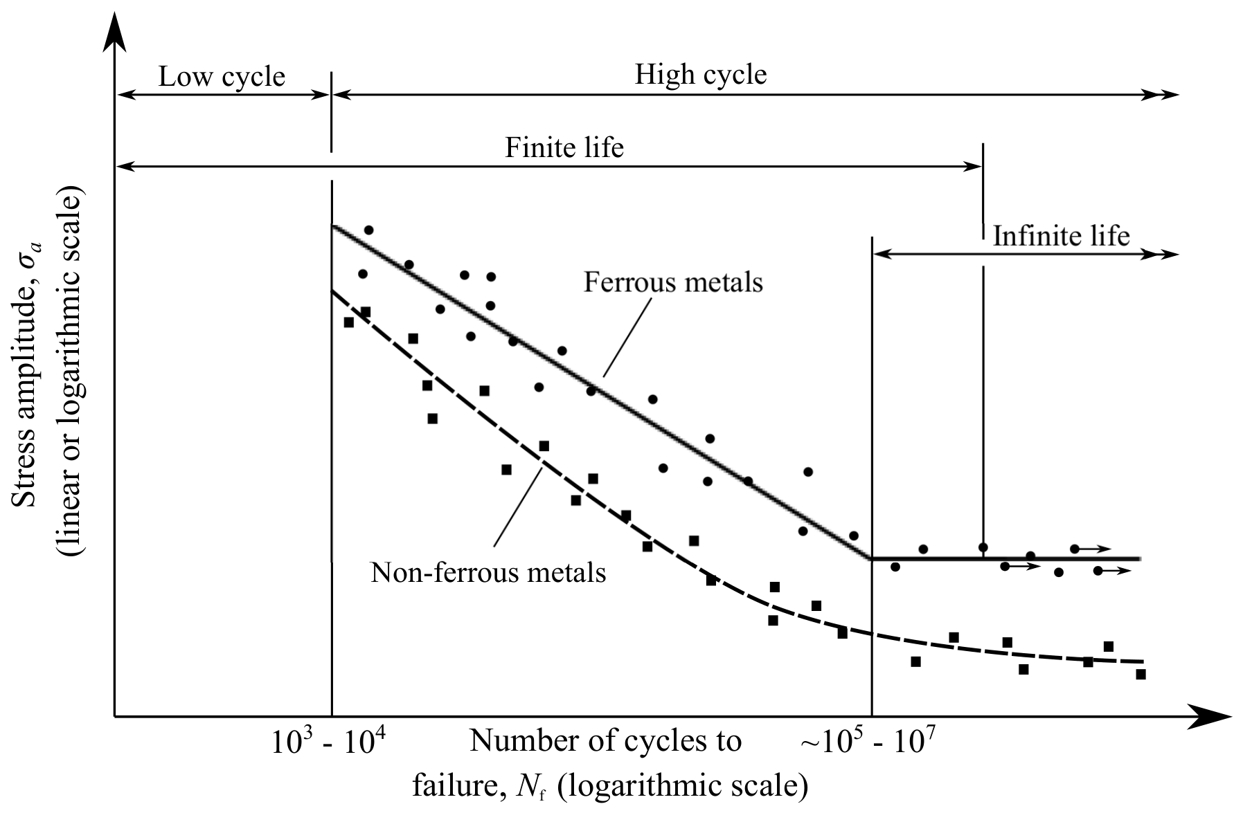
Figure 2.
Schematic representation of the stress concentration and fatigue notch factors.
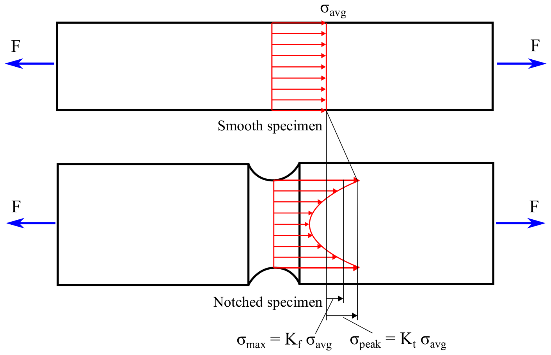
Figure 3.
Schematic representation of the Gerber, Goodman, Soderberg and Morrow mean correction models.
Figure 3.
Schematic representation of the Gerber, Goodman, Soderberg and Morrow mean correction models.
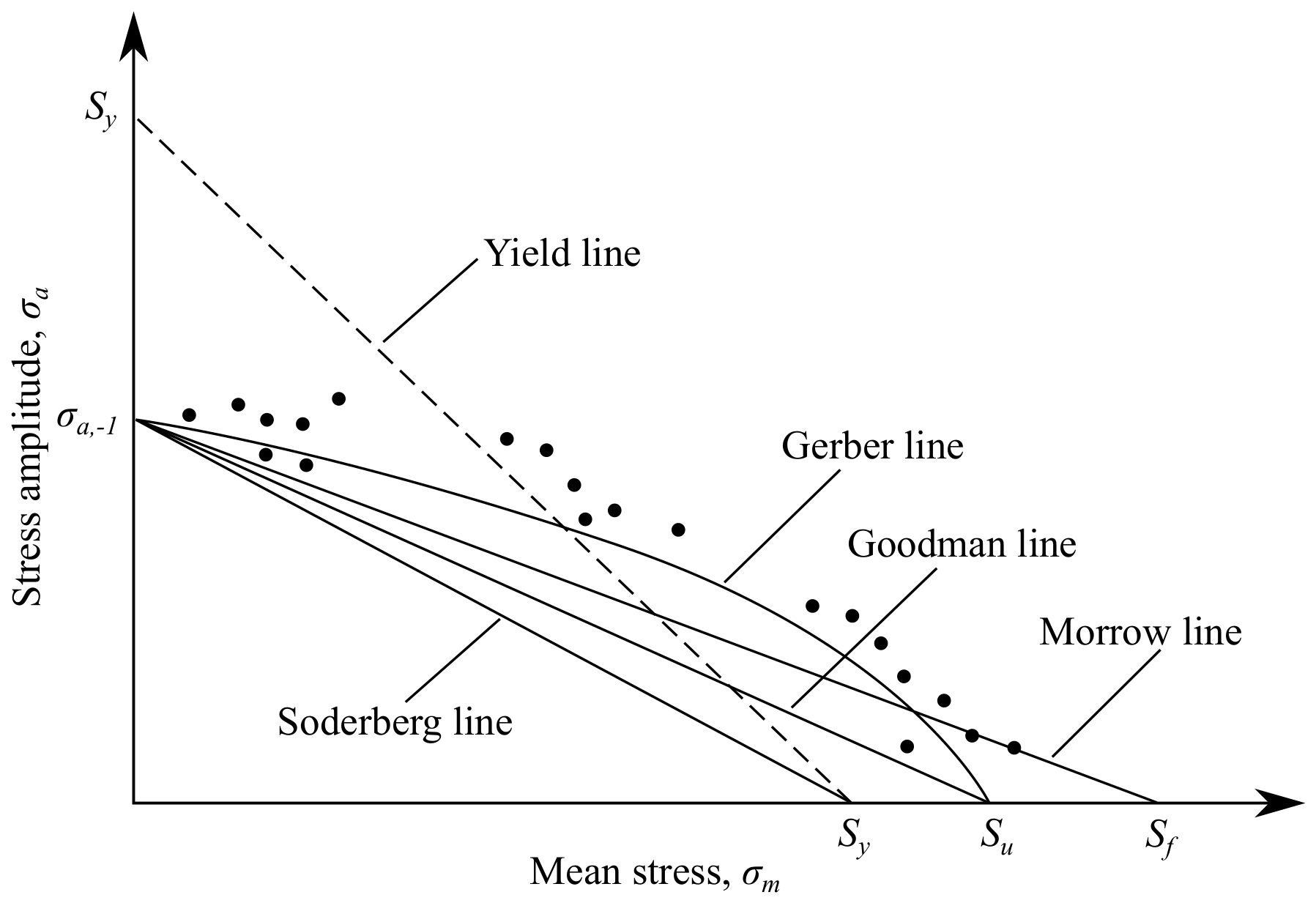
Figure 4.
Fatigue analysis of variable stress amplitude: (a) rain-flow cycle procedure and (b) the corresponding percentage damage accumulated in each block of cyclic load [48].
Figure 4.
Fatigue analysis of variable stress amplitude: (a) rain-flow cycle procedure and (b) the corresponding percentage damage accumulated in each block of cyclic load [48].
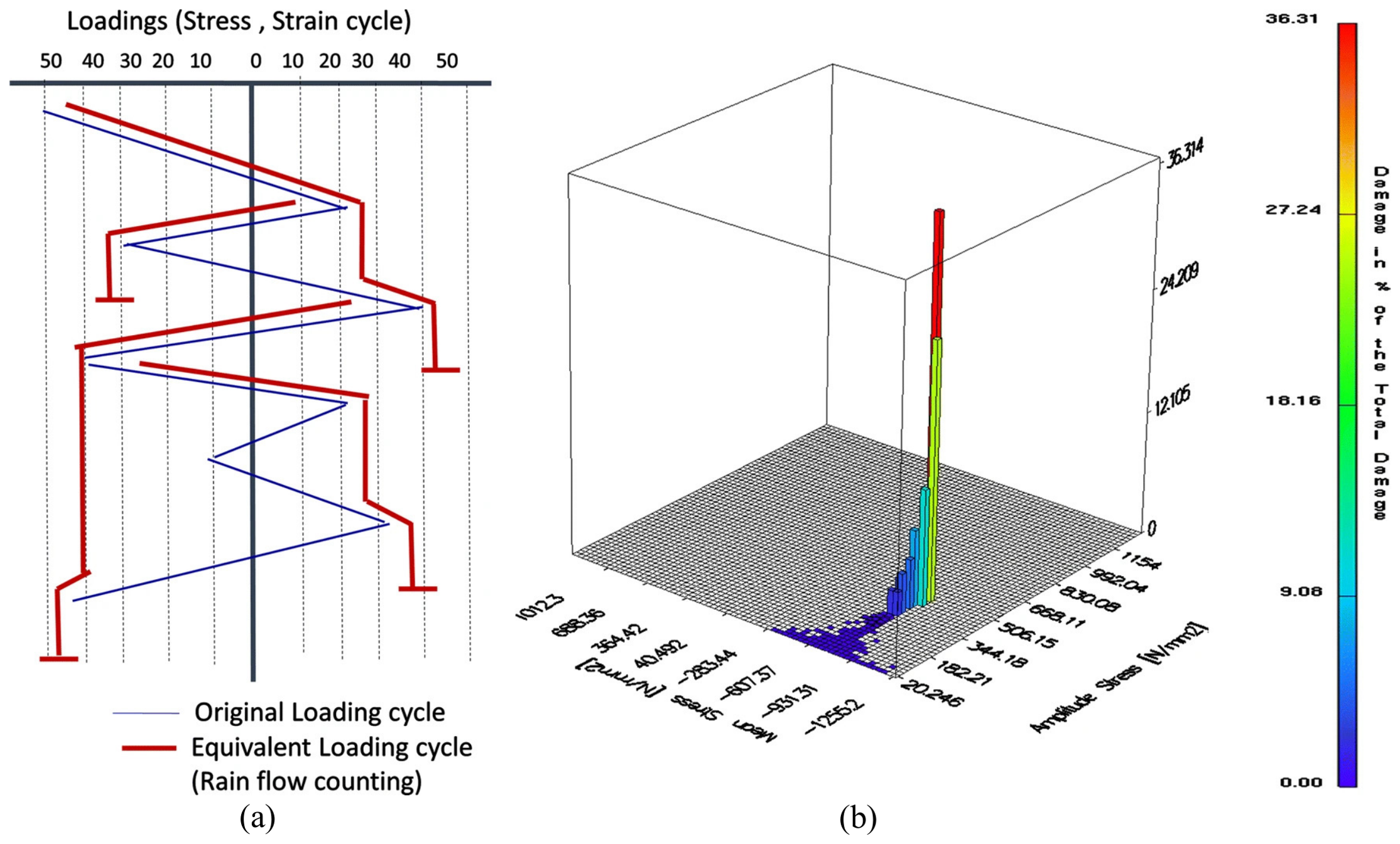
Figure 5.
Examples of fatigue plot results obtained as a post-processing operation of a linear elastic FEA: (a) accumulated damage [49], (b) number of cycles [48] and (c) safety factor [50].
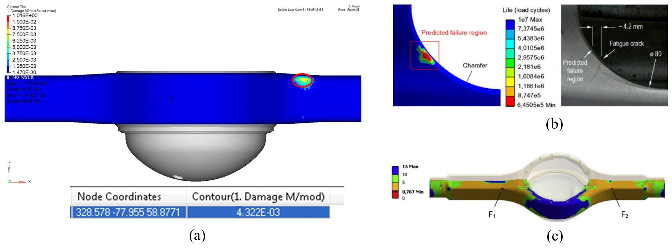
Figure 6.
Schematic representation of a stable hysteresis stress-strain loop.
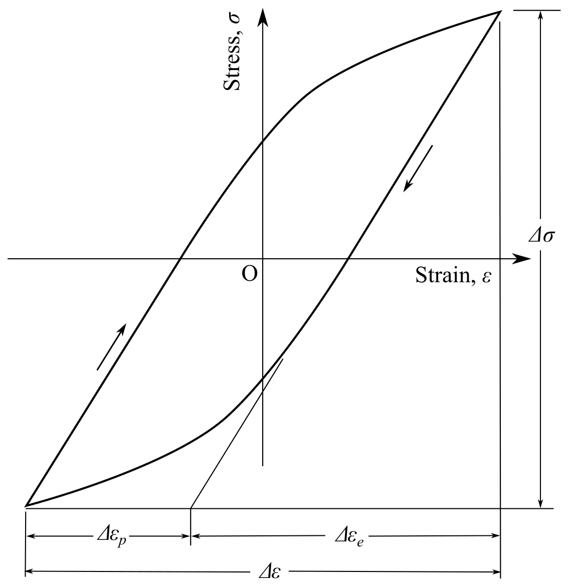
Figure 7.
Schematic representation of a strain amplitude-number of reversals curve.
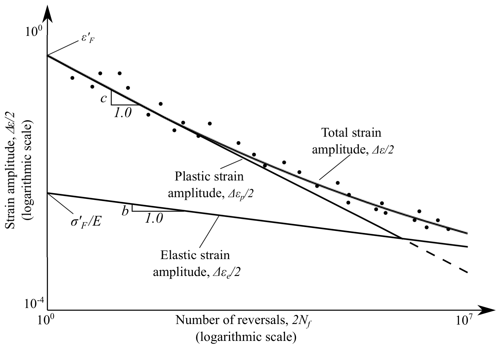
Figure 8.
Fundamental crack propagation modes
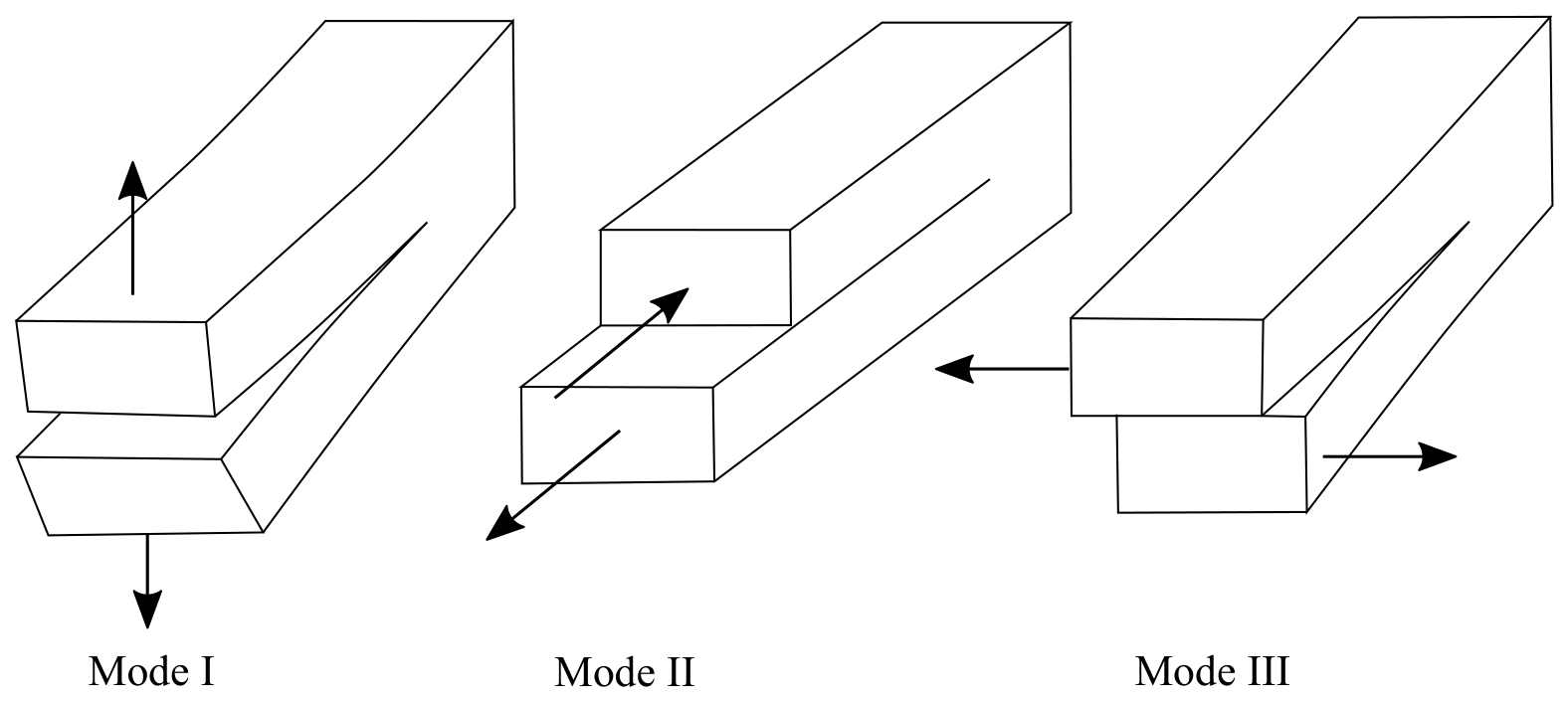
Figure 9.
Schematic representation of a typical crack growth curve
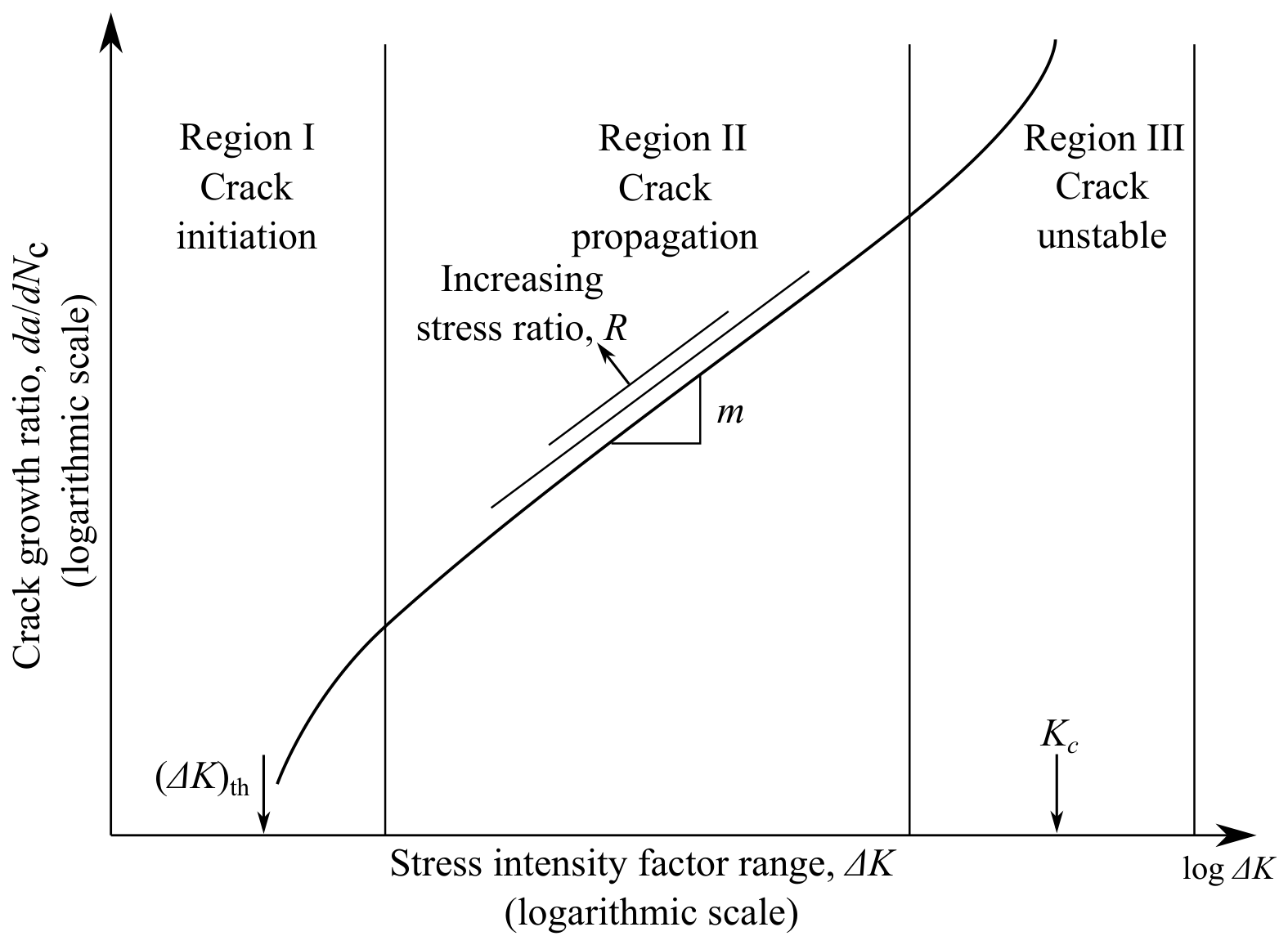
Figure 10.
Sharp discontinuity representation: (a) domain with a crack , (b) displacement field and (c) strain field.
Figure 10.
Sharp discontinuity representation: (a) domain with a crack , (b) displacement field and (c) strain field.
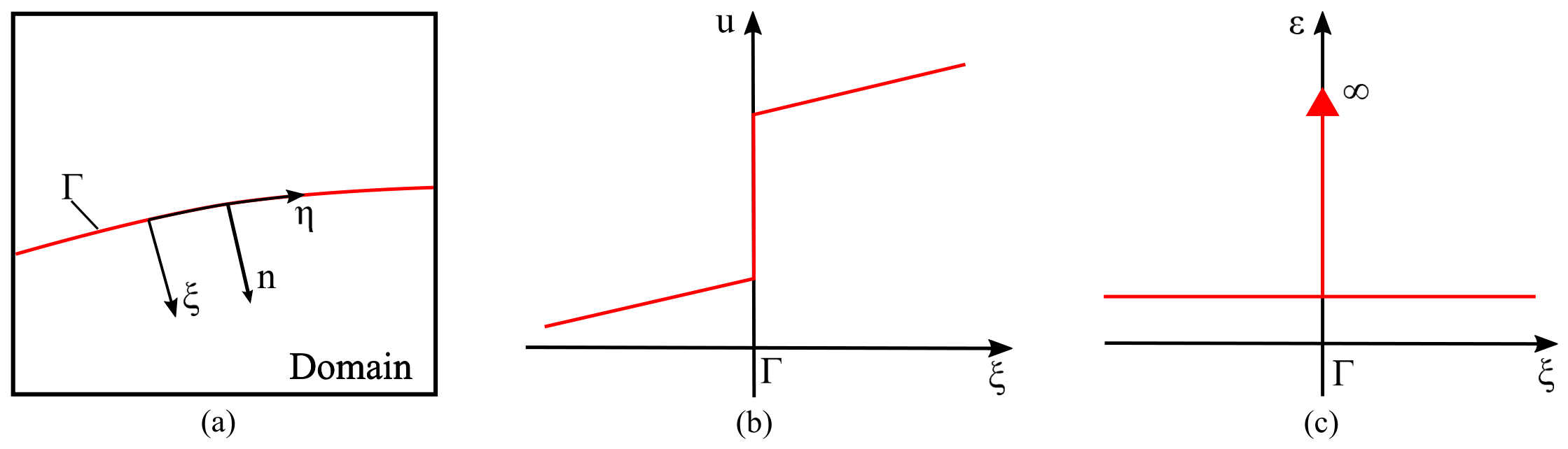
Figure 11.
Typical steps of local remeshing techniques: (a) previous mesh, (b) removal of the elements around the crack and crack advance, (c) creation of the rosette of elements around the crack tip and (d) remeshing of the blank area [77].
Figure 11.
Typical steps of local remeshing techniques: (a) previous mesh, (b) removal of the elements around the crack and crack advance, (c) creation of the rosette of elements around the crack tip and (d) remeshing of the blank area [77].
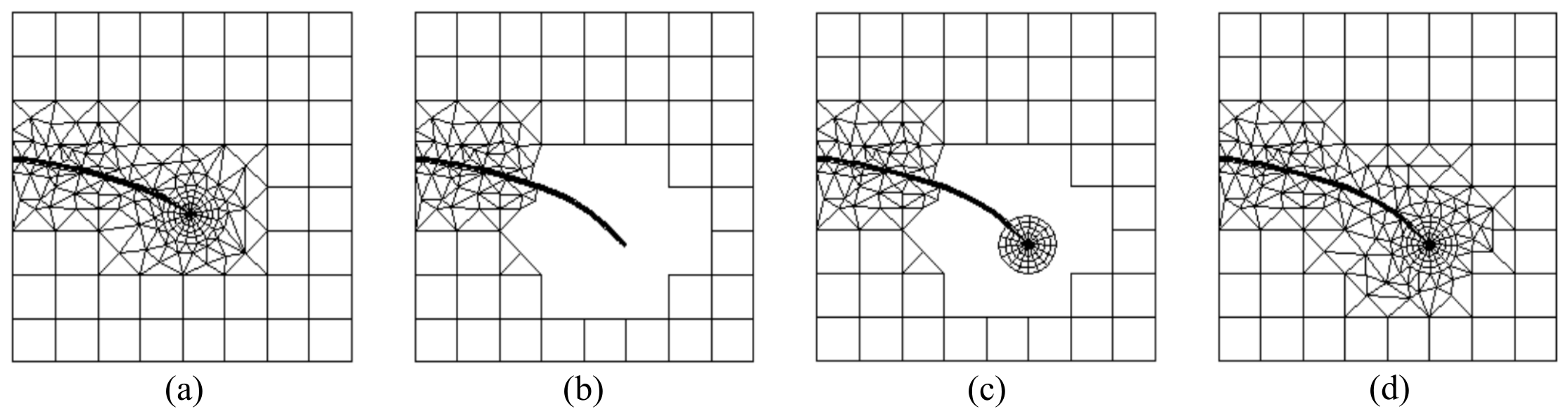
Figure 12.
Steps of an optimized local remeshing technique: (a) elements intersected by the crack increment, , in the previous mesh, (b) removal of the intersected elements (c) creation of triangular elements in the open area and (d) debonding of the corresponding nodes along the crack faces. Adapted from [76].
Figure 12.
Steps of an optimized local remeshing technique: (a) elements intersected by the crack increment, , in the previous mesh, (b) removal of the intersected elements (c) creation of triangular elements in the open area and (d) debonding of the corresponding nodes along the crack faces. Adapted from [76].
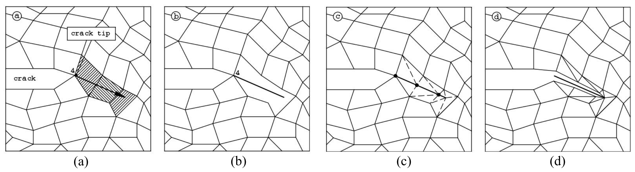
Figure 13.
Crack representation in an XFEM setting. Blue square and red circles represent step and crack tip enriched node, respectively [105].
Figure 13.
Crack representation in an XFEM setting. Blue square and red circles represent step and crack tip enriched node, respectively [105].
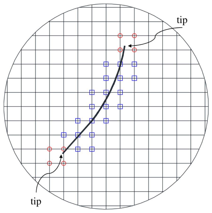
Figure 14.
Crack representation through the level set method: (a) signed-distance function defining the crack geometry and position, (b) signed-distance function determining the crack fronts and (c) domain with the resulting crack. Adapted from [77].
Figure 14.
Crack representation through the level set method: (a) signed-distance function defining the crack geometry and position, (b) signed-distance function determining the crack fronts and (c) domain with the resulting crack. Adapted from [77].
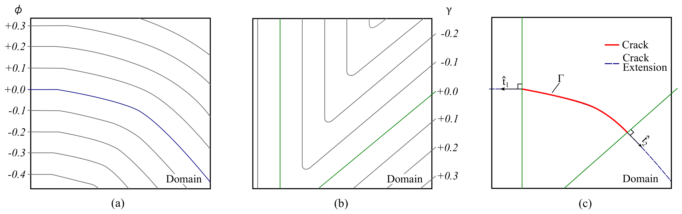
Figure 15.
Schematic representation of the domain originally covered by the continuum damage theory and its interface with fracture mechanics. Adapted from [111].
Figure 15.
Schematic representation of the domain originally covered by the continuum damage theory and its interface with fracture mechanics. Adapted from [111].
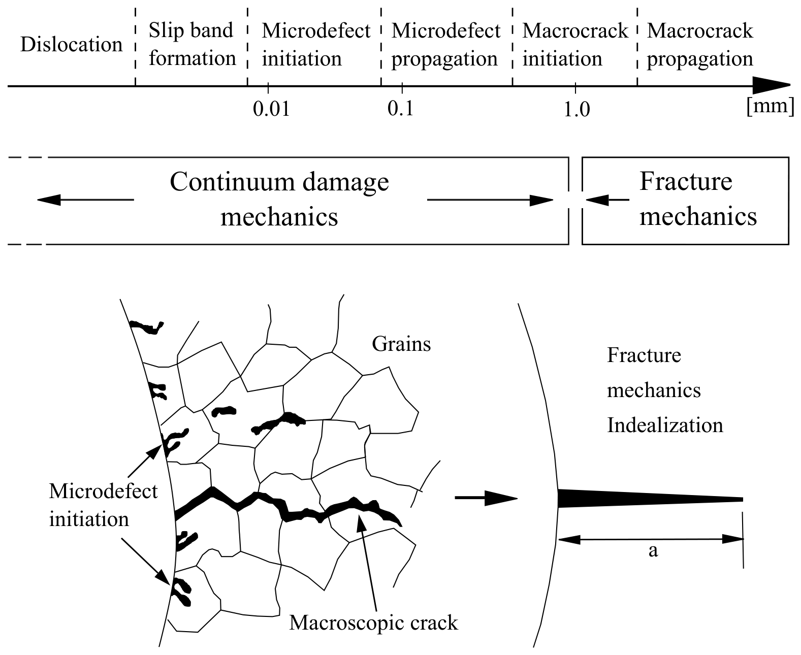
Figure 16.
Regularized representation of a discontinuity: (a) domain with the fracture process zone, including the crack idealization at the locus of critical damage, , (b) displacement field and (c) strain field.
Figure 16.
Regularized representation of a discontinuity: (a) domain with the fracture process zone, including the crack idealization at the locus of critical damage, , (b) displacement field and (c) strain field.
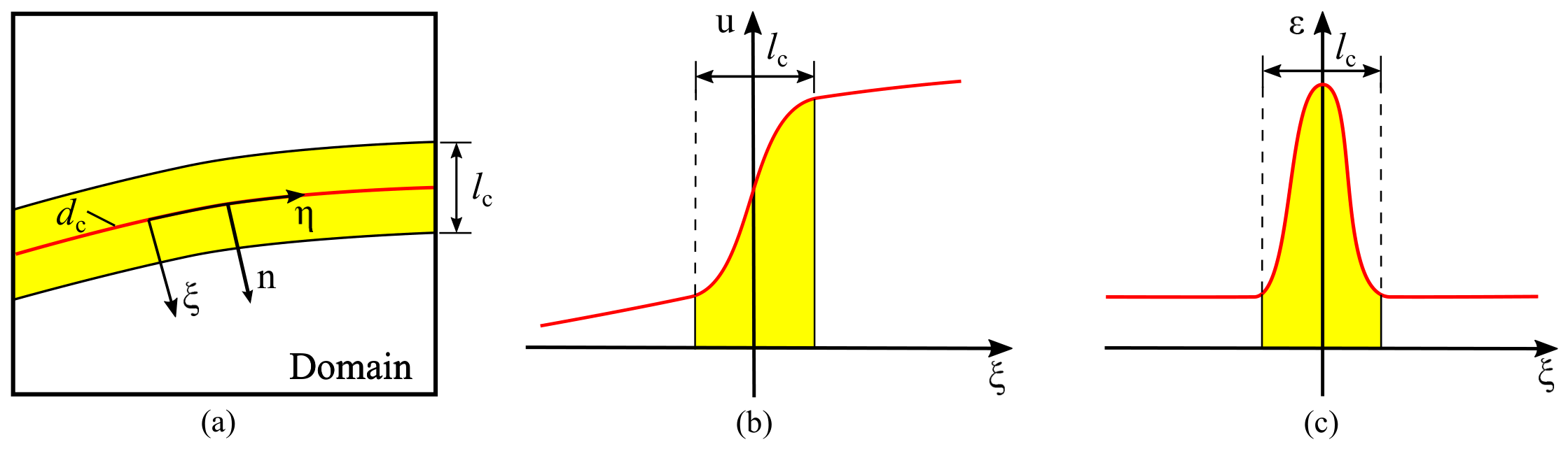
Figure 17.
Uniaxial stress-strain curves for damage: (a) linear softening and (b) exponential softening. Adapted from [120].
Figure 17.
Uniaxial stress-strain curves for damage: (a) linear softening and (b) exponential softening. Adapted from [120].
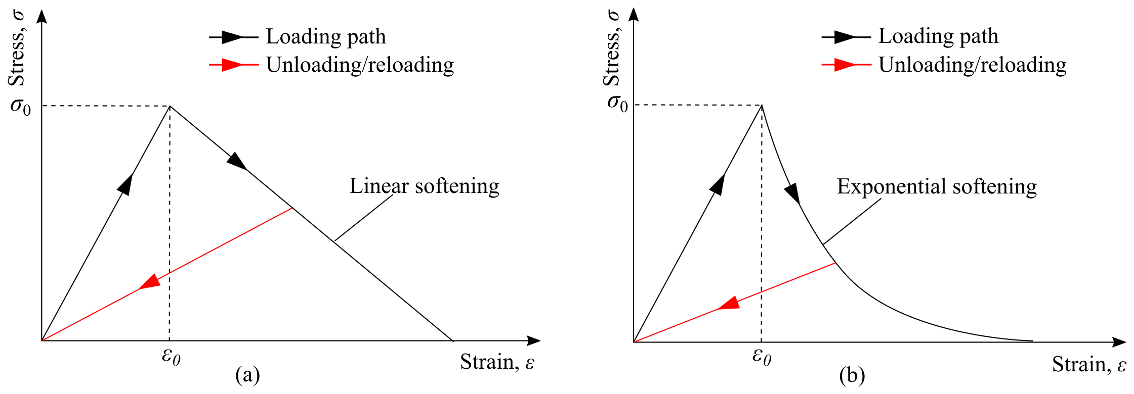
Figure 18.
Schematic representation of the Bažant size effect
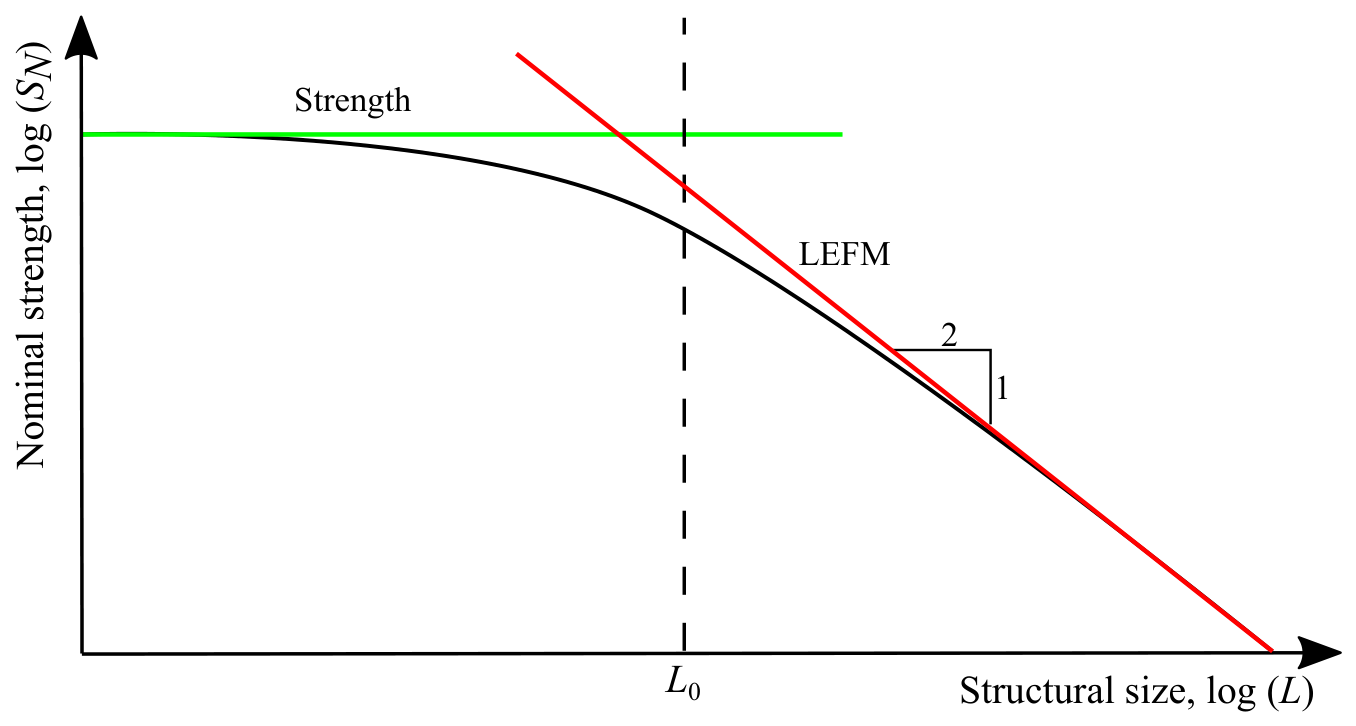
Figure 19.
Force-crack opening displacement (CMOD) response obtained from Grégoire’s tests on fifth-notched beams together with the predictions of smeared crack models [122].
Figure 19.
Force-crack opening displacement (CMOD) response obtained from Grégoire’s tests on fifth-notched beams together with the predictions of smeared crack models [122].
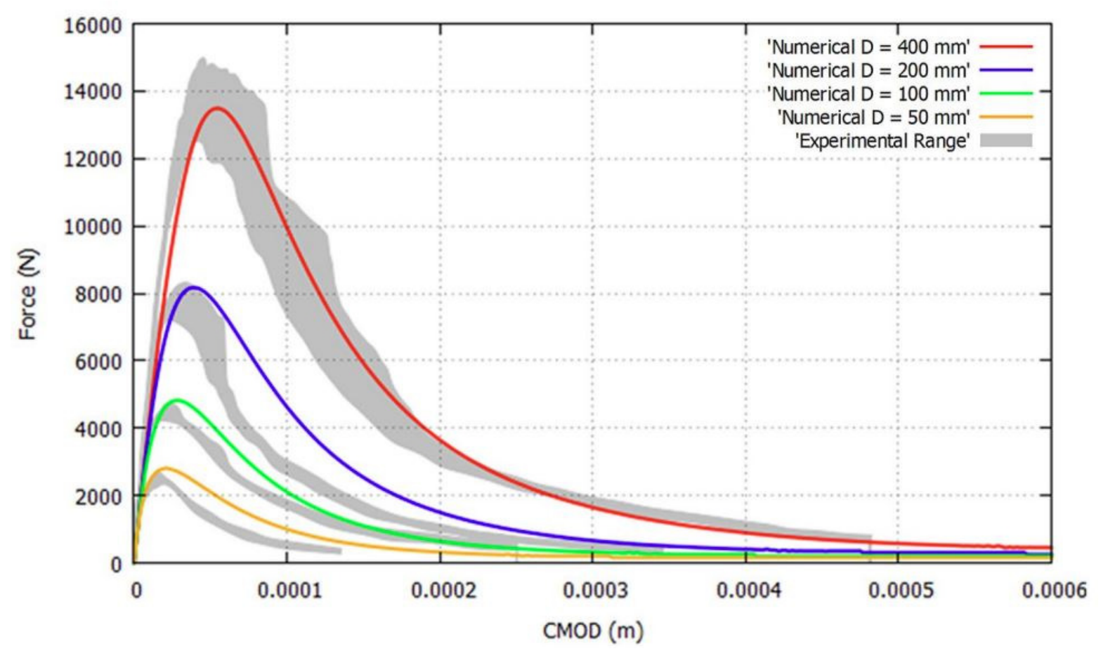
Figure 20.
Schematic representation of the effective stress concept: (a) real space and (b) effective space. Adapted from [125].
Figure 20.
Schematic representation of the effective stress concept: (a) real space and (b) effective space. Adapted from [125].
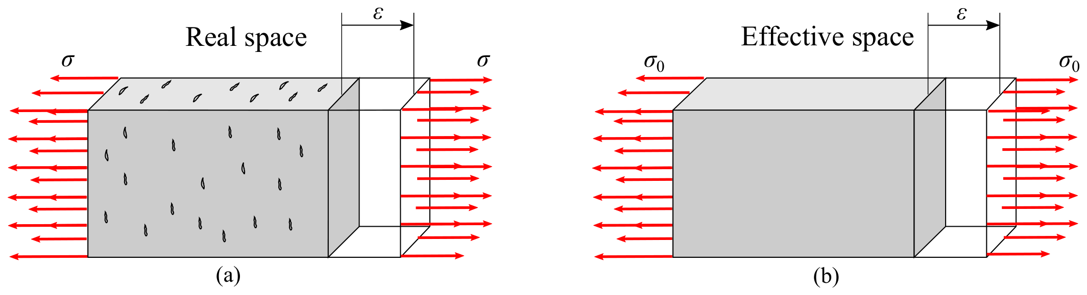
Figure 21.
Schematic representation of the body with: (a) a sharp discontinuity and (b) the corresponding phase-field approximation. Adapted from [209].
Figure 21.
Schematic representation of the body with: (a) a sharp discontinuity and (b) the corresponding phase-field approximation. Adapted from [209].
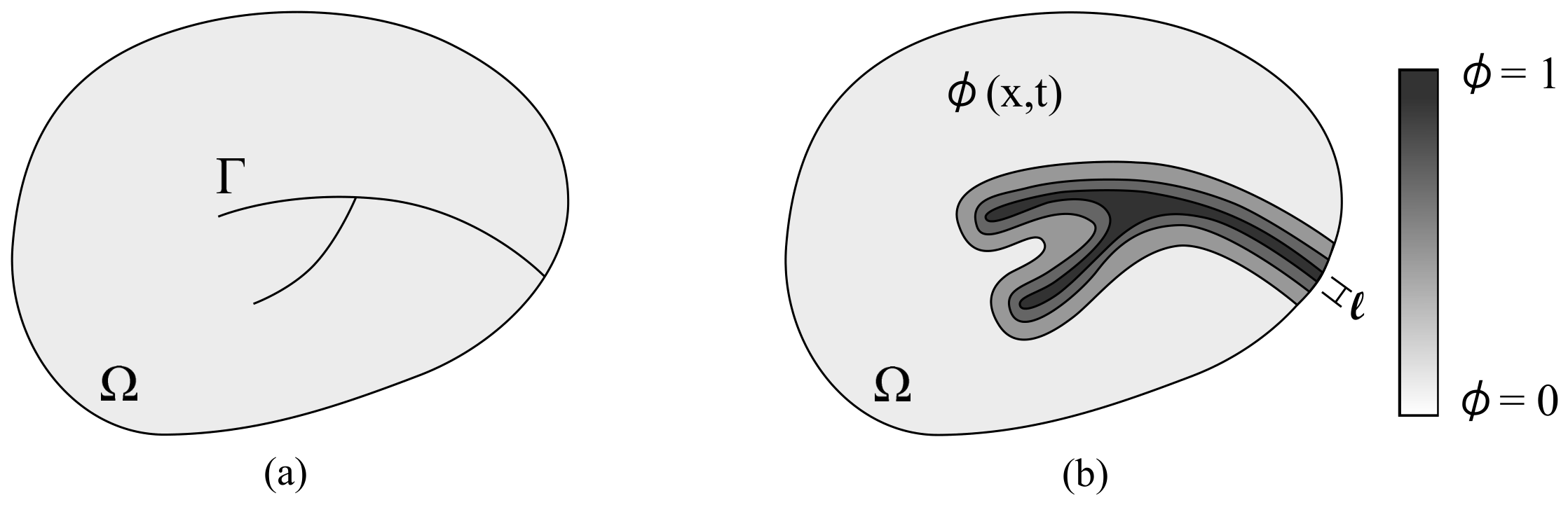
Figure 22.
Uniaxial stress-strain response predicted by the AT1 and AT2 formulations for the crack surface density function [213].
Figure 22.
Uniaxial stress-strain response predicted by the AT1 and AT2 formulations for the crack surface density function [213].
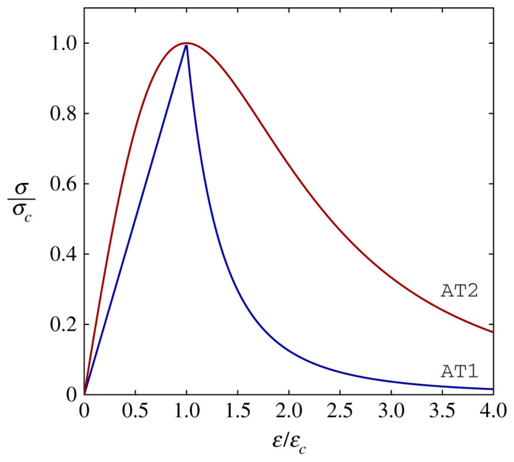
Figure 23.
Size effects predicted by the formulations: (a) AT1 and (b) AT2 . The solid lines represent the theoretical predictions based on the material strength and Griffith’s criterion, whereas the markers denote the corresponding phase-field results. Sources [213].
Figure 23.
Size effects predicted by the formulations: (a) AT1 and (b) AT2 . The solid lines represent the theoretical predictions based on the material strength and Griffith’s criterion, whereas the markers denote the corresponding phase-field results. Sources [213].
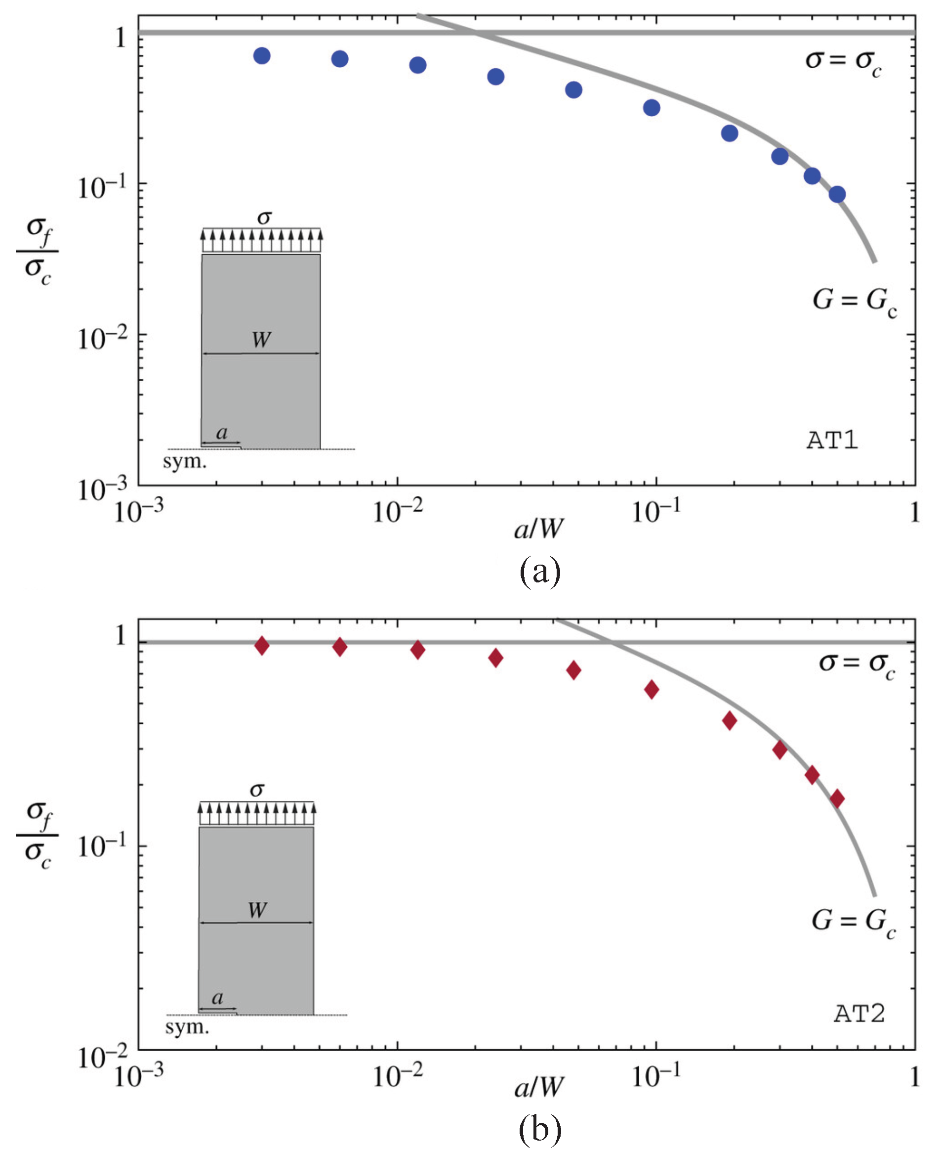
Figure 24.
Tension–compression splits of the elastic strain energy density under fatigue loading using the (a) volumetric–deviatoric [214], (b) spectral [208] and (c) no-tension [215] formulations [216].
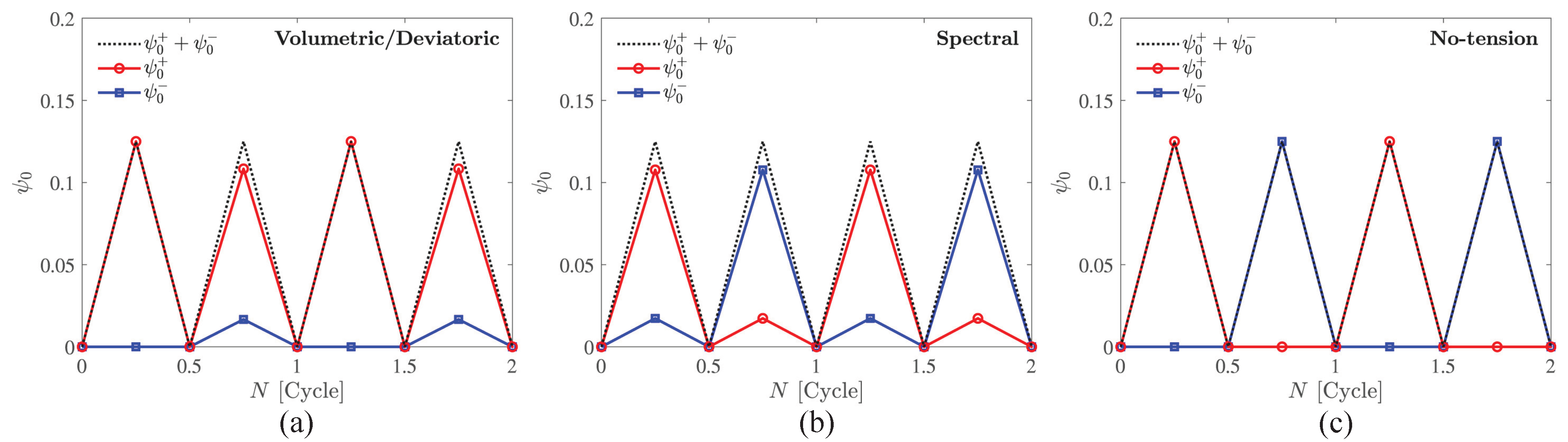
Figure 25.
Fatigue degradation functions (a) asymptotic and (b) logarithmic for different [47].
Figure 25.
Fatigue degradation functions (a) asymptotic and (b) logarithmic for different [47].
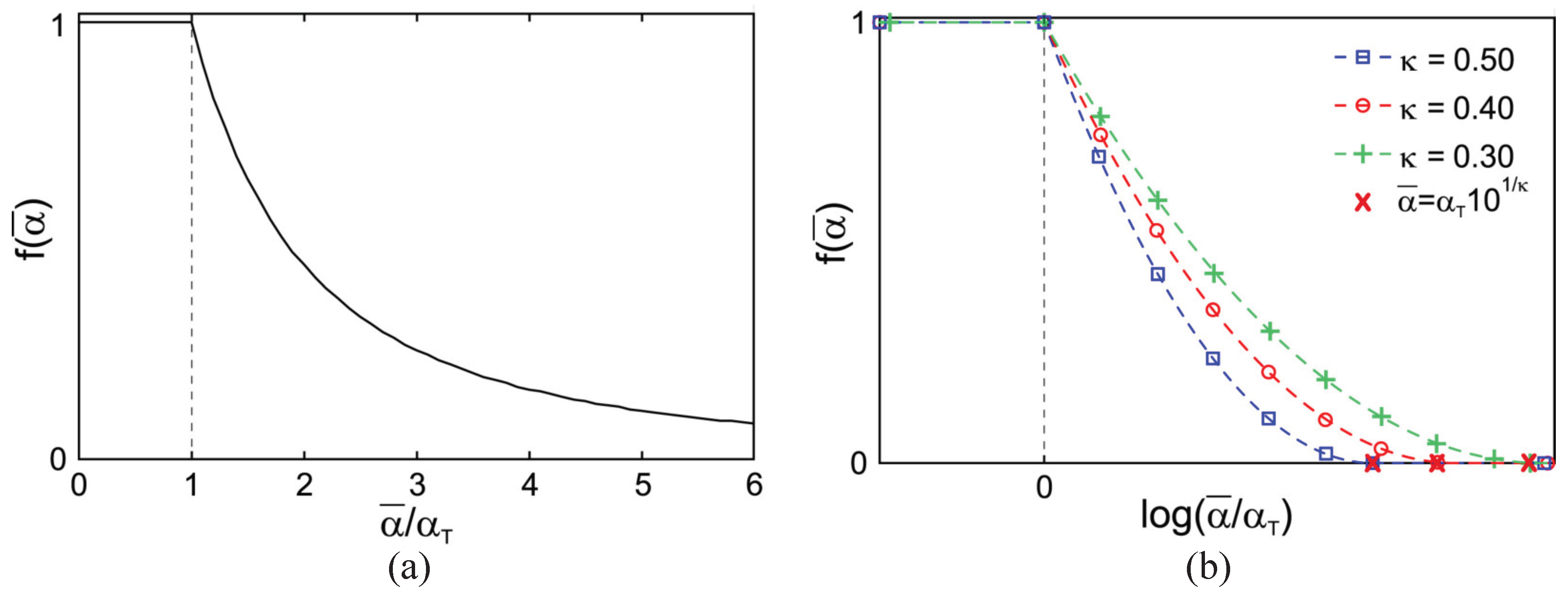
Figure 26.
Cyclic stress of constant amplitude and respective fatigue accumulation quantities, and [216].
Figure 26.
Cyclic stress of constant amplitude and respective fatigue accumulation quantities, and [216].
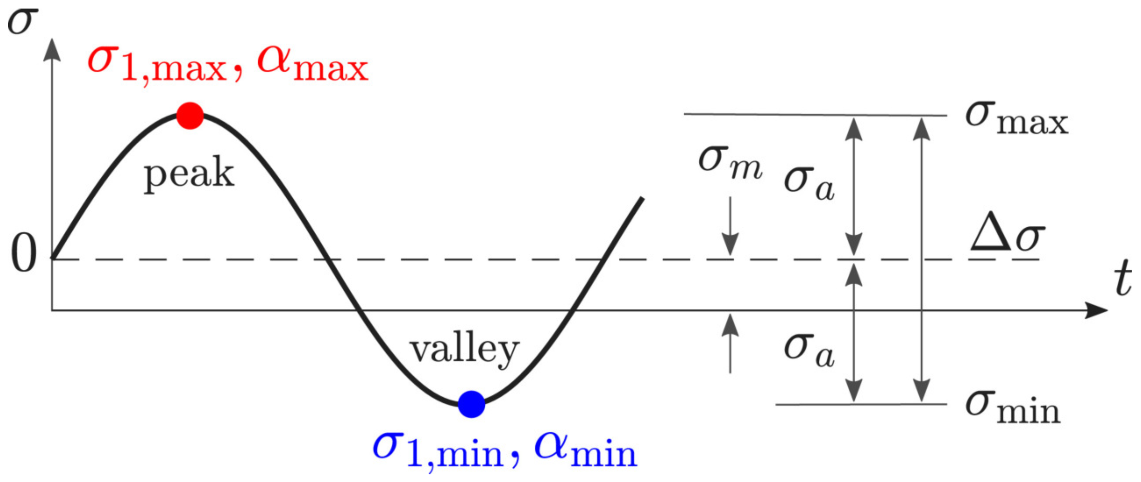
Figure 27.
Fatigue simulation acceleration strategies: (a) load application approaches and (b) fatigue history variable accumulation schemes. Adapted from [217].
Figure 27.
Fatigue simulation acceleration strategies: (a) load application approaches and (b) fatigue history variable accumulation schemes. Adapted from [217].
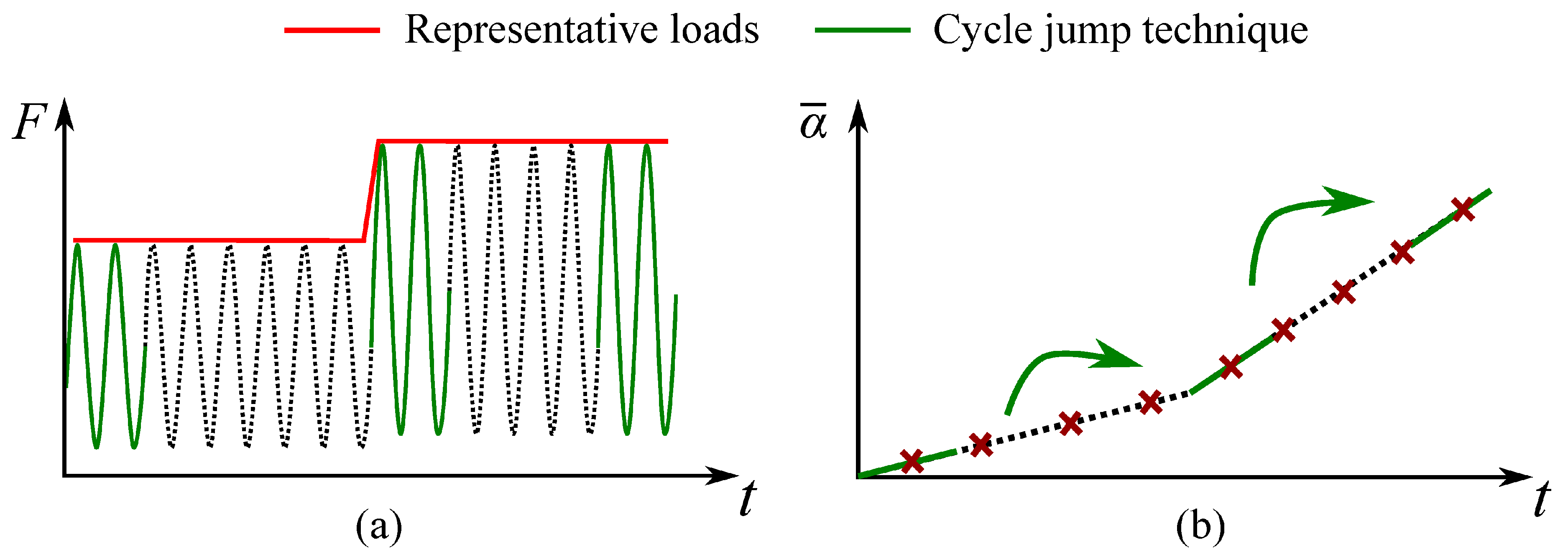
Figure 28.
Numerical reproduction of the Arrea and Ingraffea beam test using: (a) FM with XFEM, (b) CDM with a mixed finite element formulation and (c) PF model. Adapted from [232].
Figure 28.
Numerical reproduction of the Arrea and Ingraffea beam test using: (a) FM with XFEM, (b) CDM with a mixed finite element formulation and (c) PF model. Adapted from [232].
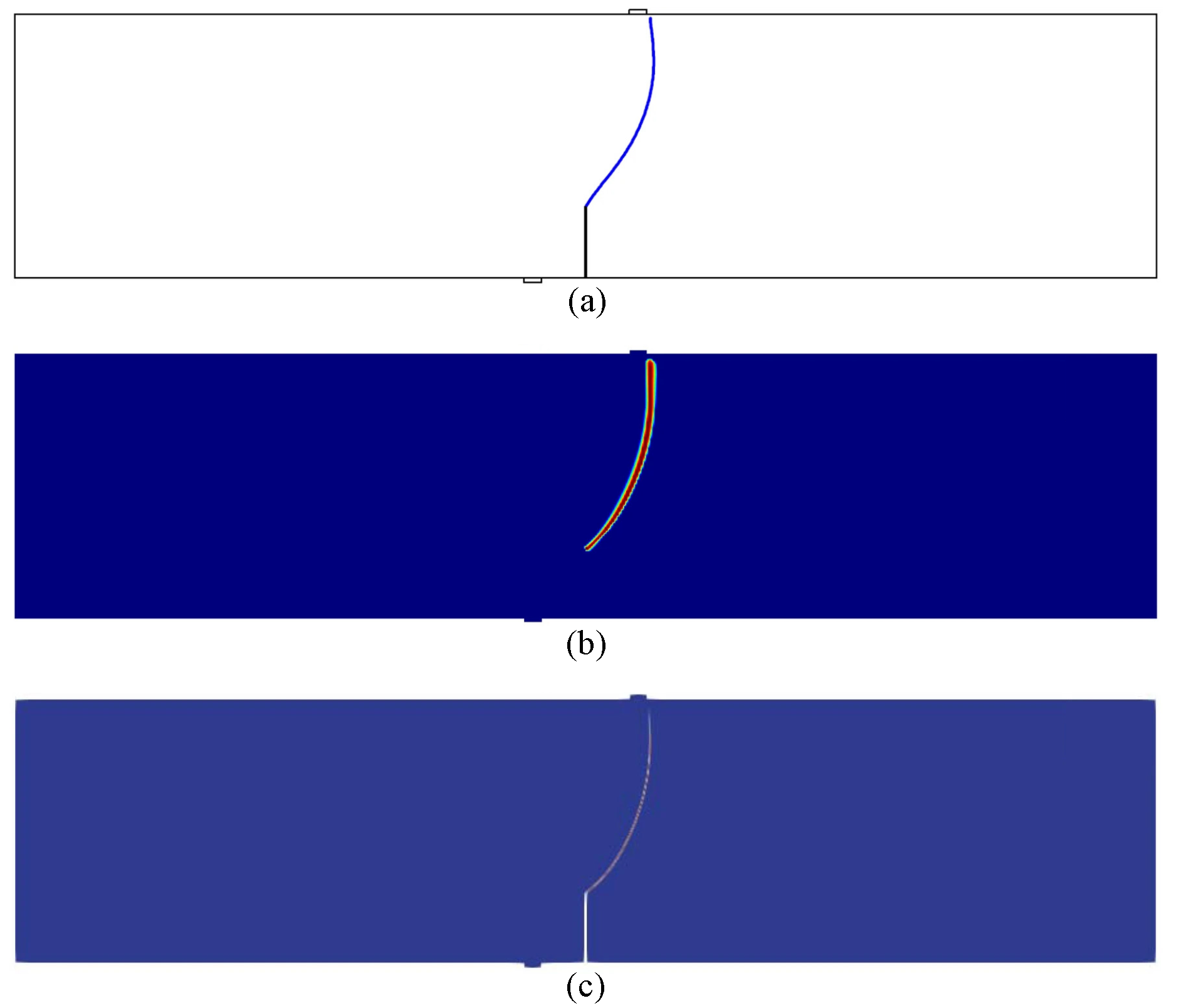

Table 1.
Mean stress correction models. Stress amplitudes at () and at a given R (), mean stress (), ultimate tensile strength (), yield stress (), true fracture strength (), Walker’s model parameter (), Kowfie’s model parameter () and Sekercioglu’s model parameter (k).
Table 1.
Mean stress correction models. Stress amplitudes at () and at a given R (), mean stress (), ultimate tensile strength (), yield stress (), true fracture strength (), Walker’s model parameter (), Kowfie’s model parameter () and Sekercioglu’s model parameter (k).
| Model | Equation | Material parameters |
|---|---|---|
| Gerber [30] | ||
| Goodman [31] | ||
| Smith [32] | ||
| Soderberg [33] | ||
| Marin [35] | ||
| Morrow [34] | ||
| Walker [36] | ||
| Smith–Watson–Topper [37] | – | |
| Dietmann [38] | ||
| Kwofie [39] | , | |
| Sekercioglu [40] | , k |
1Widely known as SWT mean stress correction model.
Table 2.
Classification of material damage, microscopic mechanisms and characteristic features.
| Damage | Microscopic mechanisms, characteristic features, etc. |
|---|---|
| Elastic damage [126,127,128,129,130,131] | Nucleation and growth of microscopic cracks caused by the elastic deformation of the matrix. Rocks, concrete, composites and metals. |
| Elastic–plastic damage [120,126,129,132,133,134,135,136,137,138,139,140] | Nucleation and growth of microscopic voids caused by elastic–plastic deformation of the matrix. Intersection of slips, particle decohesion and particle cracking. Metals, composites and polymers. |
| Spall damage [155,156,157,158] | Elastic and elastic–plastic damage due to impulsive loads. Uniform distribution of microscopic voids and cracks. Coupling between void growth and stress waves. |
| Fatigue damage [120,126,131,132,141,142,143,144,145,146,147,148,149,150,151,152] | Transgranular microscopic surface cracks caused by repeated loading. |
| Creep damage [159,160,161,162] | Nucleation and growth of microscopic intergranular voids and cracks caused by creep, mainly due to grain-boundary sliding and diffusion. |
| Creep–fatigue damage [131,161,163,164,165,166,167] | Damage induced by repeated loading at high temperature. Nonlinear coupling between intergranular voids and transgranular cracks. |
| Corrosion damage [126,129,132,136,153] | Pitting corrosion, intergranular corrosion and development of microcracks under stress in corrosive environments. |
| Irradiation damage [132,160,164] | Damage caused by neutron, particle and -ray irradiation. Knock-on of atoms, nucleation of voids and bubbles, and swelling. |
Table 3.
Fatigue damage evolution laws. Young’s modulus (E), Poisson’s ratio (), current yield stress (), ultimate tensile strength (), material fatigue limit (), fully reversed fatigue limit (), uniaxial stress (), maximum and minimum stresses ( and ), mean stress (), hydrostatic stress (), von Mises equivalent stress (), strain range (), plastic strain range (), stress triaxiality (), stress ratio (R), number of cycles to failure at low and high frequency ( and ), damage at low (creep–fatigue) and high frequency (pure fatigue) ( and ) and damage thermodynamic conjugate (Y). Model-specific parameters: Chaboche–Lesne , Lemaitre–Plumtree , Paas and Peerlings , Xiao , Fu , Dufailly et al. , Lemaitre et al. .
Table 3.
Fatigue damage evolution laws. Young’s modulus (E), Poisson’s ratio (), current yield stress (), ultimate tensile strength (), material fatigue limit (), fully reversed fatigue limit (), uniaxial stress (), maximum and minimum stresses ( and ), mean stress (), hydrostatic stress (), von Mises equivalent stress (), strain range (), plastic strain range (), stress triaxiality (), stress ratio (R), number of cycles to failure at low and high frequency ( and ), damage at low (creep–fatigue) and high frequency (pure fatigue) ( and ) and damage thermodynamic conjugate (Y). Model-specific parameters: Chaboche–Lesne , Lemaitre–Plumtree , Paas and Peerlings , Xiao , Fu , Dufailly et al. , Lemaitre et al. .
| Model | Equation | Model parameters |
|---|---|---|
| Chaboche and Lesne [187] | , , , a, | |
| Lemaitre and Plumtree [163] | p, q, r, | |
| Paas et al. [143] | C, , | |
| Peerlings et al. [188] | C, , | |
| Xiao et al. [145] | p, q, | |
| Fu et al. [152] | , , p, | |
| Dufailly et al. [144] | s, S | |
| Lemaitre et al. [146] | C, k, s |
Table 4.
Qualitative comparison of fracture-based approaches for fatigue analysis.
| Feature | FM (XFEM) | CDM (Mixed FEM) | PF |
|---|---|---|---|
| Variational formulation at continuum level | Partial1 | Yes | Yes |
| Energy consistency with Griffith’s theory | Yes | Yes2 | Yes |
| Structural size effect | No | Yes | Yes |
| Crack initiation modelling | No | Yes | Yes |
| Crack propagation modelling | Yes | Yes | Yes |
| Mixed-mode crack growth | Requires propagation criterion | Implicit | Implicit |
| Multiple crack nucleation | Limited | Yes | Yes |
| Crack branching and merging | Limited | Yes | Yes |
| Need for crack tracking/remeshing | Yes | No | No |
| Mesh-objective crack trajectories | Conditional3 | Yes | Yes |
| Extension to fatigue | Natural for propagation | Natural | Natural |
| Life-estimation capability | Limited4 | Yes | Yes |
| Computational cost | Low | Moderate | High |
| Applicability to large 3D problems | High | Moderate–High | Limited |
1 Although fracture mechanics is founded on energy-based variational principles, practical FM formulations generally rely on additional crack-initiation and propagation criteria that are not derived from a unified variational framework. 2 Through appropriate calibration of the softening law to reproduce the fracture energy 3 Typically requires enrichment, tracking algorithms, or remeshing strategies. 4 Since crack initiation is not explicitly represented in classical fracture mechanics formulations.
Disclaimer/Publisher’s Note: The statements, opinions and data contained in all publications are solely those of the individual author(s) and contributor(s) and not of MDPI and/or the editor(s). MDPI and/or the editor(s) disclaim responsibility for any injury to people or property resulting from any ideas, methods, instructions or products referred to in the content. |
© 2026 by the authors. Licensee MDPI, Basel, Switzerland. This article is an open access article distributed under the terms and conditions of the Creative Commons Attribution (CC BY) license (http://creativecommons.org/licenses/by/4.0/).
Copyright: This open access article is published under a Creative Commons CC BY 4.0 license, which permit the free download, distribution, and reuse, provided that the author and preprint are cited in any reuse.


