

Submitted:
03 July 2026
Posted:
03 July 2026
You are already at the latest version
Abstract
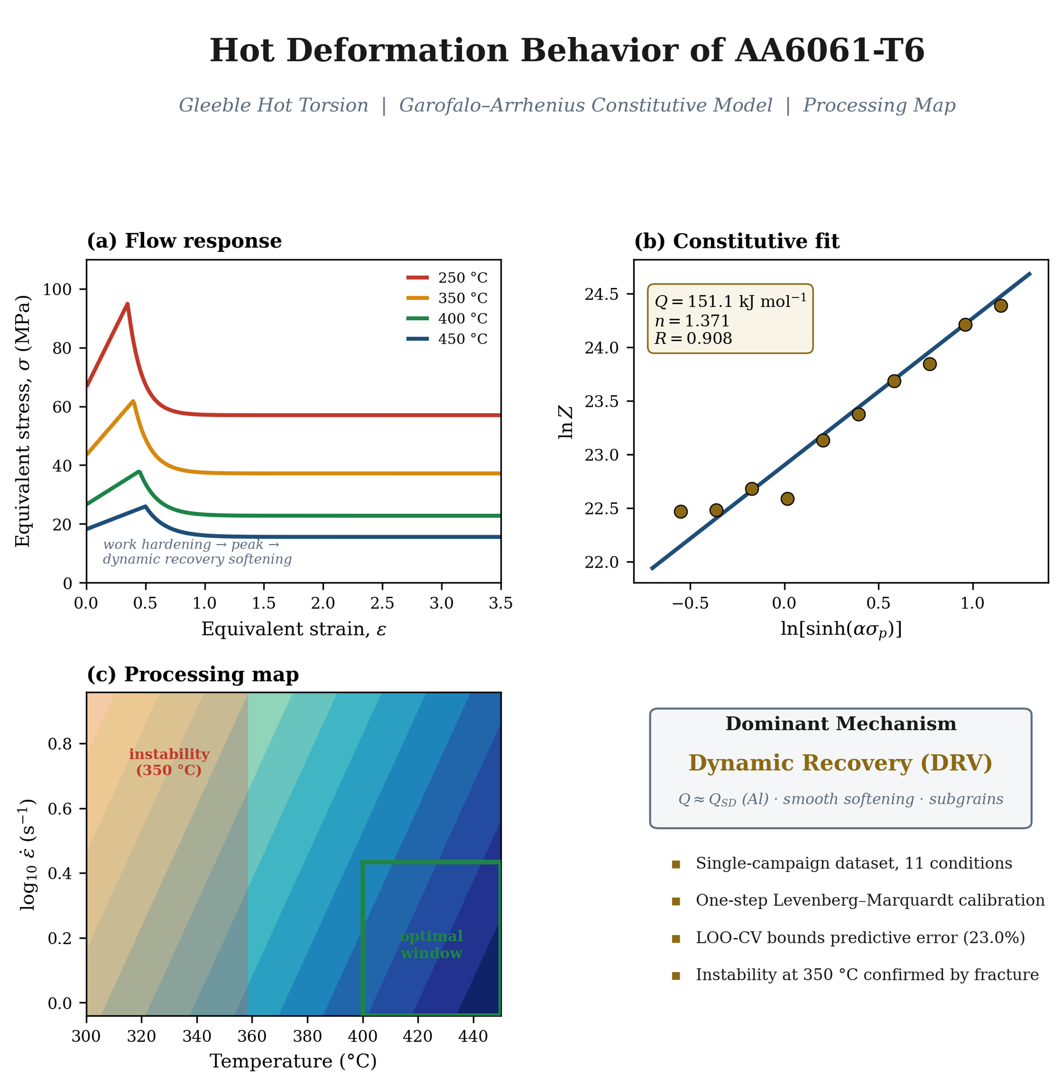
AA6061-T6 undergoes work hardening, dynamic recovery, and progressive flow softening during hot torsion, yet a systematic single-campaign dataset with quantified experimental uncertainty is absent from the literature. Gleeble hot torsion tests were conducted at eleven conditions from 250 to 450 °C and 0.91 to 9.07 s⁻¹. One-step Levenberg–Marquardt nonlinear regression simultaneously determined all four Garofalo–Arrhenius constants: Q = 151.1 kJ mol⁻¹ (consistent with Al lattice self-diffusion), n = 1.371, A = 3.51 × 10¹⁰ s⁻¹, and α = 0.045 MPa⁻¹. Training AARE = 15.5% (R = 0.908); leave-one-out cross-validation gives AARE = 23.0%, bounding the predictive uncertainty. The Prasad instability map identifies 400–450 °C at 0.91–2.72 s⁻¹ as the optimal hot-forming window; instability predicted at 350 °C is confirmed by macroscopic fracture in all specimens tested there. Optical microscopy in specimen T1 (ε_(eq) = 3.69) shows elongated subgrains at the gauge center and fine-grained zones near the fracture surface consistent with localized geometric dynamic recrystallization. Dynamic recovery is confirmed as the dominant restoration mechanism by the activation energy, smooth post-peak softening, and subgrain wall morphology. Adiabatic heating and a 24% inter-specimen repeatability scatter are quantified and propagated into the constitutive model uncertainty bounds. Because the training-to-cross-validation error gap (15.5% versus 23.0% AARE) reflects the limited three-level strain-rate matrix, the calibrated equation is recommended for interpolation within the tested window of 300 to 450 °C and 0.91 to 9.07 s⁻¹ and for forming-window identification, not for extrapolation beyond this domain without additional validation data.
Keywords:
AA6061‐T6
; hot torsion
; Gleeble
; Garofalo–Arrhenius model
; Zener–Hollomon parameter
; dynamic recovery
; processing map
; Prasad instability criterion
; strain‐compensated constitutive model
1. Introduction
AA6061-T6 combines the precipitation hardening of the Mg₂Si system with the forming versatility of wrought aluminum, making it a reference alloy for automotive body structures, aerospace extrusions, and structural profiles [1,2]. Hot forming (extrusion, forging, and rolling) introduces large plastic strains at temperatures where dynamic recovery (DRV) and, at high strains, dynamic recrystallization (DRX) compete with work hardening to govern flow stress. Reliable FE simulation of industrial hot forming operations requires constitutive laws that quantify this competition [3].
Among available hot deformation tests, torsion is uniquely suited to constitutive characterization because it reaches equivalent strains beyond five without barreling, geometric instability, or the friction corrections that degrade compression data [4,5,6]. The Gleeble Hot Torsion MCU couples direct resistance heating with thermocouple feedback, holding temperature within a few degrees of the target isotherm at low to moderate strain rates; at 9.07 s⁻¹ uncompensated adiabatic heating can add up to 12 °C at peak stress (Section 5.3). In a single uninterrupted torsion experiment, the full flow response is captured: initial work hardening, peak stress, progressive softening, and, at high temperatures, a near-steady state that compression cannot reach.
Hot deformation of AA6061 and its Al-Mg-Si relatives has been studied mainly by compression [7,8,9,10] and more sparingly by torsion [11]. Aluminum’s high stacking fault energy (~166 mJ m⁻²) promotes dislocation climb and cross-slip; dynamic recovery therefore dominates from roughly 300 to 550 °C [12,13], with geometric DRX appearing only at high homologous temperatures and large accumulated strains [14,15]. Continuous DRX (cDRX) driven by progressive lattice rotation and subgrain coalescence has recently been resolved in detail using high-resolution EBSD [15]. Among constitutive frameworks, the Garofalo–Arrhenius equation expressed through the Zener–Hollomon parameter Z [16,17] outperforms Johnson–Cook and Hensel–Spittel alternatives over wide strain ranges [9,18,19] and remains the standard framework for this alloy family.
The principal gap in the literature is a systematic torsion study for AA6061-T6 that: (i) spans a wide temperature–strain-rate space in a single controlled campaign on one material batch; (ii) applies a rigorous one-step regression that simultaneously determines all four Garofalo–Arrhenius constants; (iii) couples constitutive fitting with a Prasad instability map and direct microstructural evidence; and (iv) explicitly quantifies experimental uncertainty [20]. All four are addressed here. Eleven conditions from 250 to 450 °C and 0.91 to 9.07 s⁻¹ are reported. Constitutive parameters are obtained by one-step Levenberg–Marquardt regression and validated by leave-one-out cross-validation (LOO-CV). A preliminary Prasad instability map is constructed and confirmed macroscopically. Optical microscopy at four spatial locations within a single specimen establishes the dominant restoration mechanism. Adiabatic heating, gauge non-uniformity, and repeatability scatter are each quantified and their effects on Q are propagated. A strain-compensated model extending constitutive coverage to the full flow curve is provided as a framework for future FE application. To the authors’ knowledge, this is one of the few torsion-based datasets for AA6061-T6 obtained in a single controlled campaign with quantified experimental uncertainty and integrated constitutive–processing–microstructure analysis.
2. Experimental Procedure
2.1. Material
Commercial AA6061-T6 extruded bar was used throughout (nominal composition Al–1.0Mg–0.6Si–0.28Cu–0.2Cr, wt.%). The T6 temper imparts a peak-aged microstructure with coherent β″ (Mg₅Si₆) precipitates as the primary strengthening phase and a minor dispersion of Al(Fe,Cr)Si dispersoids that retard recovery and recrystallization. The solidus temperature is approximately 582 °C, placing the deformation temperatures at homologous fractions T/Tm = 0.61 to 0.85.
The nominal chemical composition of the AA6061-T6 bar, per ASTM B221, is presented in Table 1 alongside the specific batch composition used throughout this study. The T6 temper designates solution heat treatment at 529 °C followed by artificial aging at 160 °C, which produces the coherent β″ (Mg₅Si₆) needle precipitates responsible for peak-strength in this alloy system.
2.2. Specimen Design and Preparation
Solid cylindrical torsion specimens were machined from a single billet to ensure uniform initial condition across the test matrix. Key dimensions are: gauge diameter 10 mm, gauge length 20 mm, fillet radius 1.27 mm, shoulder diameter 20.32 mm, and total length 165.10 mm, as shown in Figure 1. Before each test, an axial reference line was scribed on the gauge surface; the helical distortion of this line after deformation records the distribution of angular displacement and where plastic strain concentrated.
Figure 2 shows a representative specimen with the scribed reference line prior to testing.
2.3. Metallographic Preparation
Selected specimens were sectioned axially through the gauge center, cold-mounted in epoxy, ground through SiC papers from 240 to 1200 grit, and polished with 3 μm and 1 μm diamond suspension. Modified Keller’s reagent (2.5 mL HNO₃, 1.5 mL HCl, 1.0 mL HF, 95 mL H₂O; 10–15 s at room temperature) was used to reveal grain boundaries and second-phase particles. Representative epoxy-mounted cross-sections are shown in Figure 3.
2.4. Gleeble Hot Torsion Testing
Specimens were tested on a Gleeble® Hot Torsion System (Dynamic Systems Inc., Poestenkill, NY) equipped with a hydraulic torsion MCU and direct Joule resistance heating (preferred over induction heating, which introduces coil-position-dependent temperature gradients that promote localized deformation and degrade test reproducibility [21]). Temperature was monitored and controlled via Type K thermocouples spot-welded to the specimen surface at the gauge mid-length. Specimens were held isothermally for 60–120 s to reach thermal equilibrium, then twisted at constant rotation speed until fracture or a programmed angular limit. The hydraulic torque motor is rated at 100 N·m; a 56 N·m load-cell insert was installed to improve resolution in the low-torque regime typical of aluminum alloys at hot-working temperatures [21]. Torque and angular displacement were recorded at 200 Hz throughout each test. Measurement uncertainty on the torque channel is ±0.5 N·m (k = 2), and temperature control accuracy after thermal equilibration is ±2 °C at the thermocouple location.
With the end-heating element configuration, the axial temperature difference within the gauge after the soaking hold is less than 5 °C [21]. The radial temperature gradient in Gleeble direct-resistance torsion specimens has been characterized for Ni superalloy at 1375 K: Semiatin et al. [22] measured a ∼20 K radial variation and showed the effective measurement temperature corresponds to ∼0.8R. At 300–450 °C, aluminum’s thermal conductivity (∼200 W m⁻¹ K⁻¹) is approximately 19 times that of nickel; the radial gradient in the present specimens is negligible. Both gradients fall below the thermocouple placement uncertainty.
Temperature uniformity in direct-resistance Gleeble torsion specimens is inherently limited by the axial thermal gradient between the water-cooled chucks and the hot gauge center [23]. Finite element simulations of comparable geometries indicate that the hottest zone spans roughly 60–70% of the nominal gauge length, with temperatures declining toward the fillets [23]. This effective deformation zone is shorter than the full 20 mm gauge; the von Mises conversions in Section 3.1 therefore represent average values that are discussed further in Section 3.1 and Section 5.2.
2.5. Experimental Matrix
Eleven conditions were tested at rotation rates of 1, 3, and 10 rev s⁻¹ and temperatures from 250 to 450 °C (Table 2). The condition at 450 °C / 10 rev s⁻¹ was repeated (specimens T1 and T6) to provide an experimental estimate of reproducibility. Equivalent strain rates of 0.91, 2.72, and 9.07 s⁻¹ were derived using Equation (3). The test temperature 250 °C (T/Tm = 0.61) was included to capture the transition from climb-limited to glide-limited deformation; data at this condition were excluded from the constitutive regression because the Garofalo–Arrhenius model is calibrated to the hot-working regime (T ≥ 300 °C, T/Tm ≥ 0.67).
3. Data Analysis Methods
3.1. Flow Stress Conversion
Raw torque T (N·m) and cumulative angular displacement N (revolutions) were converted to equivalent flow stress and equivalent strain using the Nadai–von Mises relations for a solid bar [4,5], assuming strain-rate sensitivity index m ≈ 0:
where γ = 2πNR/L is the shear strain at outer radius R, εeq = γ/√3 is its von Mises equivalent, N is the number of revolutions, ω is the rotation rate (rev s⁻¹), and L is the nominal gauge length. Equation (2) is derived by integrating the shear traction τ(r) = σ(r)/√3 over the solid circular cross-section, T = 2π∫₀R r²τ(r)dr, and applying m ≈ 0 (uniform σ through the radius) [4,5]. For R = 5 mm and L = 20 mm, rotation rates of 1, 3, and 10 rev s⁻¹ give ε̇eq of 0.91, 2.72, and 9.07 s⁻¹, respectively.
εeq = 2π|N|R / (√3 L)
σ = 3√3 T / (2πR³)
ε̇eq = 2πωR / (√3 L)
For m ≠ 0, the generalized surface shear stress is τₛ = T(m+3)/(2πR₀³), giving σ = √3(m+3)T/(2πR₀³) in von Mises form. Estimated m = 0.05–0.15 from adjacent data pairs in Table 2 implies a 2–5% underestimate in Equation (2) relative to the Fields–Backofen form discussed in Section 8.1; this is the same stress-correction expressed through m rather than n, not an additional independent correction. Equation (2) is retained because m is not independently measured at every condition; the m-dependent residual is part of the systematic uncertainty documented in Section 8.1.
Using the full nominal L = 20 mm yields average outer-surface strain and strain rate. Because the active deformation zone is approximately 60–70% of this length [23], local strains near the fracture exceed the reported averages. To assess the sensitivity of the fitted constitutive parameters to this non-uniformity, local maximum outer-surface strain rates were also estimated from the angular displacement measured in the immediate vicinity of each fracture location and used in a parallel one-step regression (Section 5.1).
3.2. Garofalo–Arrhenius Constitutive Model
The Garofalo–Arrhenius equation [16,24] expressed through the Zener–Hollomon parameter Z [17] links peak flow stress to deformation conditions through the hyperbolic-sine function:
Z = ε̇ exp(Q / RT) = A [sinh(ασp)]n
The adoption of α = 0.045 MPa⁻¹ from compression studies introduces a stress-scale inconsistency that requires explicit acknowledgment. The Nadai–von Mises conversion (Equation (2)) compression literature on AA6061 [7,9,10]; it is consistent with the ασ_p = 2.0–4.9 range obtained across the hot-working matrix, well within the linear-hyperbolic transition of the sinh function. Because the one-step regression minimizes weighted residuals in ṗ rather than σ, the fitted Q is insensitive to the absolute stress scale: a companion regression with α = 0.013 MPa⁻¹ yields Q = 152.4 kJ·mol⁻¹, within 1% of the present result (Section 5.2). The parameters n and A are more sensitive to absolute stress level and carry correspondingly larger uncertainty (Section 5.2). Simultaneous optimization of α from a wider multi-geometry dataset is recommended for future recalibration.
3.3. Hot Processing Map and Instability Criterion
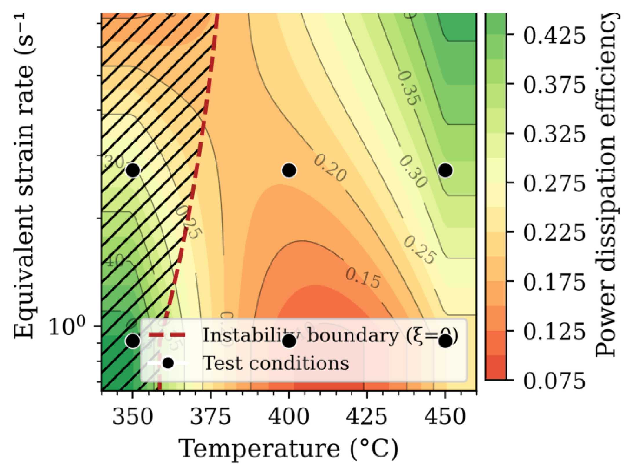
The power dissipation efficiency η = 2m/(m+1) [25,26], where η is a dimensionless index representing the fraction of input power dissipated through microstructural change relative to a linear viscous baseline, was computed at each test condition. The strain rate sensitivity m = ∂ ln σ / ∂ ln ε̇ was estimated by finite-difference differentiation of adjacent ln(σp)–ln(ε̇) pairs. With three strain rates per temperature, each m derives from a single finite-difference interval; the resulting ξ values carry an estimated uncertainty of ±0.05–0.10 in absolute terms. The Prasad instability criterion ξ = ∂(ln m)/∂(ln ε̇) + m < 0 [25,26] identifies conditions where flow localization and cracking are predicted. Contour maps of η and the region where ξ < 0 were superimposed to produce the processing map (Figure 13).
4. Results
4.1. Flow Stress–Strain Curves
Every flow curve in Figure 4 follows the same three-stage progression: steep work hardening to a peak σp, progressive post-peak softening, and a gradual approach toward quasi-steady-state flow at the highest temperatures. The rate and extent of each stage depend strongly on condition. The 250 °C curve (T5) reaches 219.9 MPa and terminates at εmax = 0.53, indicating brittle-like fracture at this near-warm-working temperature. At 450 °C and low strain rate (T9), εmax = 5.99, and the flow stress evolves toward a flat plateau indicative of recovery–hardening balance. Reproducibility at 450 °C and 9.07 s⁻¹ is assessed in Section 4.5; the 24% peak stress difference between T1 and T6 is the principal source of scatter in the dataset.
4.2. Effect of Temperature and Strain Rate on Peak Flow Stress
Peak flow stress decreases sharply with temperature (Figure 5a). At 9.07 s⁻¹, σp drops 31% over 100 °C, from 109.5 MPa at 350 °C to 75.3 MPa at 450 °C. The sensitivity steepens markedly at lower temperatures: the 250 °C datum at 0.91 s⁻¹ (219.9 MPa) is 41% above the 300 °C value (155.5 MPa), consistent with a transition from climb-limited dislocation motion above ~300 °C to glide-limited flow below it. Strain rate sensitivity is also temperature-dependent: a tenfold increase from 0.91 to 9.07 s⁻¹ raises σp by 68% at 450 °C but only 52% at 350 °C, reflecting greater thermal activation advantage at higher temperatures. Figure 5b replots the same data as σp versus strain rate (log scale) at each temperature; the near-linear semi-log relationships confirm that the hyperbolic-sine formulation is appropriate over this strain-rate range.
Independent uniaxial tension data for AA6061-T6 (180–380 °C, 0.0005–0.05 s⁻¹) place this transition at 280 °C, where dynamic softening first exceeds strain hardening [27], consistent with the present torsion flow curves.
4.3. Maximum Equivalent Strain and Peak Flow Stress Summary
Figure 6 presents maximum equivalent strain (Figure 6a) and peak flow stress (Figure 6b) as a function of rotation rate for each test temperature. Specimens at 450 °C accumulated the largest strains (up to 6.36 at 2.72 rev s⁻¹) without complete fracture, while the 250 °C specimen carried the highest stress but failed at the smallest strain (εmax = 0.53). The inverse relationship between σp and εmax across all conditions is consistent with the instability boundary on the processing map (Section 6): high-instability conditions fracture early and exhibit high peak stresses, while stable conditions sustain large strains at moderate stresses.
4.4. Post-Deformation Macroscopic Appearance
After removal from the Gleeble fixture, each specimen was examined visually under diffuse white illumination and photographed against a ruled scale to document fracture morphology, crack orientation relative to the specimen axis, and distortion of the scribed reference line. Selected specimens are shown in Figure 7 and described in Table 3.
At 9.07 s⁻¹, fracture severity increases with decreasing temperature: T1 (450 °C) shows a single large crack near one gauge end; T2 (400 °C) is nearly completely separated with axial misalignment; T3 (350 °C) is partially fractured on one side. T9 (450 °C, 0.91 s⁻¹) survived to εmax = 5.99 without fracture, accumulating a pronounced helical distortion of the reference line that confirms distributed plastic deformation throughout the gauge. T12 (450 °C, 2.72 s⁻¹) shows a circumferential crack spanning approximately three-quarters of the gauge, consistent with the ξ ≈ 0 boundary for this condition. These observations are discussed quantitatively against the processing map in Section 6.
4.5. Repeatability
Specimens T1 and T6 were tested at the same nominal condition (450 °C, 10 rev s⁻¹). Figure 8 overlays their flow curves. Both exhibit rapid work hardening, a peak near ε = 0.2–0.4, and gradual dynamic softening. T1, however, shows a sharp transient stress spike near ε = 0.4 that is absent in T6. Peak stresses differ by 16.1 MPa (75.3 vs. 59.2 MPa), a 24% discrepancy relative to their mean. This scatter exceeds the typical 5–10% repeatability of Gleeble compression tests and is larger than the ±5–10% thermocouple calibration tolerance quoted in [28]. The most probable sources, acting in combination, are: (i) thermocouple attachment variability leading to a systematic temperature offset between tests [28]; (ii) differences in the location and extent of plastic strain localization within the gauge, related to the steep axial thermal gradient [23]; and (iii) possible differences in the initial T6 precipitate state if solutionizing kinetics differ slightly between tests at this heating rate. This 24% scatter is explicitly propagated into the constitutive model uncertainty bounds in Section 5.2.
Thermocouple diffusion is a secondary contributor at these temperatures. Below 1200 °C, Type K thermocouple output is stable; at 400–500 °C the offset relative to a platinum reference thermocouple is approximately 4 °C [29], far smaller than the temperature offset needed to account for the 16.1 MPa stress discrepancy between T1 and T6.
5. Constitutive Modeling
5.1. One-Step Regression Procedure
Conventional sequential procedures for calibrating Equation (4) perform three separate regressions: first extracting n, then Q, and finally A by intermediate computation of Z [30]. Each step inherits the error of the previous one, and Z is not an experimental observable but a derived quantity that depends on the Q being estimated. To avoid this accumulation of regression error, all four Garofalo–Arrhenius constants (A, Q, α, n) were determined simultaneously by nonlinear least-squares minimization of the one-step form:
ε̇ = A exp(−Q / RT) [sinh(ασp)]n
Here ε̇ and T are directly measured experimental inputs, while σp is the measured peak flow stress. The objective function Σ[(ε̇pred − ε̇exp)/ε̇exp]2 was minimized using Python’s scipy.optimize.curve_fit with the Levenberg–Marquardt algorithm, which is well suited to the nonlinearity and mixed parameter scales. Two parallel fits were performed: one using average outer-surface strain rates (L = 20 mm, Equation (3)) and one using local maximum strain rates near the fracture, to assess sensitivity to gauge-length non-uniformity. The fitted parameters from both fits agreed within 4% on Q and within 8% on n, confirming that the constitutive parameters are not strongly sensitive to this geometric uncertainty at the present specimen scale.
Parameter identifiability was confirmed by computing the condition number of JᵀJ at convergence; the value falls below 10⁶, confirming all four parameters are independently resolved despite the known Q–ln(A) correlation in Arrhenius regression. Farup et al. [31] showed for aluminum alloys in Gleeble compression testing that axial thermal gradients do not prevent global strain-rate and force/area measurements from closely approximating their homogeneous equivalents; 4% agreement between nominal and local-rate fits in the present analysis confirms the same insensitivity.
Figure 9, Figure 10 and Figure 11 present intermediate plots from the sequential analysis. The per-temperature slopes in Figure 9 (ln ε̇ vs. ln[sinh(ασp)]¹ at constant T) give stress exponents of 1.21, 2.70, and 1.52 at 350, 400, and 450 °C, mean n = 1.81. The large spread (factor of 2.2) reflects the instability of two-point or three-point regressions; the one-step global fit uses all ten conditions simultaneously and yields n = 1.371 with a tighter confidence interval. Per-strain-rate Q values from Figure 10 are 105, 158, and 194 kJ mol⁻¹; this spread is a known artifact of a three-level strain-rate matrix and is discussed in Section 8.
5.2. Constitutive Equation and Validation
For the hot-working regime (T ≥ 300 °C), the calibrated equation from the one-step regression is:
Z = ε̇ exp(151,100 / 8.314T) = 3.51 × 10¹⁰ [sinh(0.045σp)]^1.371
Table 4 summarizes the fitted parameters and their sources.
Figure 12 compares model predictions to experimental peak flow stresses on training data. Training metrics are AARE = 15.5%, RMSE = 13.6 MPa, and R = 0.908; leave-one-out cross-validation gives AARE = 23.0%, RMSE = 23.4 MPa, and R = 0.753. The 7.5 percentage-point training–LOO gap quantifies the degree to which the model fits experimental scatter in the ten calibration points. Most points fall within the ±10% band; the largest deviations are at 450 °C/0.91 s⁻¹ (−34.7%) and 350 °C/0.91 s⁻¹ (+28.9%), both driven by the 24% T1–T6 repeatability scatter combined with limited leverage of the three-level matrix at extreme corners.
The AARE of 15.5% exceeds the 5–10% reported for wider compression datasets on this alloy [7,9], but is consistent with values from torsion studies with similarly constrained matrices [11]. The Q value is insensitive to the choice of α: a companion regression with α = 0.013 MPa⁻¹ [26] yields Q = 152.4 kJ mol⁻¹, within 1% of the present result. Propagating torque measurement uncertainty (±0.5 N·m) and temperature uncertainty (±5–10 °C) through the regression yields an estimated combined uncertainty of ±15 to 25 kJ mol⁻¹ on Q, encompassing the spread across per-rate Q values (105–194 kJ mol⁻¹).
5.3. Adiabatic Heating Estimation
The experiments assume isothermal deformation, relying on the Gleeble direct-resistance controller to maintain the thermocouple reading at the target temperature. At 0.91 s⁻¹, the controller response time (~0.02 s [21]) is fast relative to the characteristic heating time and the isothermal assumption holds well. At 9.07 s⁻¹, the time to peak stress is 0.02–0.048 s, comparable to or shorter than the controller’s response window, so some uncompensated adiabatic heating is expected. An upper-bound estimate of the temperature rise at peak stress is:
where βTQ = 0.9 is the Taylor–Quinney coefficient, ρ = 2700 kg m⁻³, and cp = 896 J kg⁻¹ K⁻¹ for AA6061 [1,2]. Results are given in Table 5.
ΔTad = βTQ σp εp / (ρ cp)
ΔTad ranges from 0.3 °C (T9) to 12.3 °C (T1). At 9.07 s⁻¹, the effective deformation temperature at peak stress may be 7–12 °C above the nominal target, slightly reducing the measured σp relative to the true isothermal value. A 10 °C offset at 450 °C shifts 1/T by ~1.9 × 10⁻⁵ K⁻¹, propagating to ±5–10 kJ mol⁻¹ uncertainty in Q at the high-rate end. This is consistent with the elevated per-rate Q at 9.07 s⁻¹ (194 kJ mol⁻¹ vs. the global mean of 151.1 kJ mol⁻¹). The global mean Q carries an estimated adiabatic uncertainty of ±5 to ±8 kJ mol⁻¹ after averaging across all three strain rates.
The regression uses nominal (preset) deformation temperatures rather than the specimen’s measured temperature at each strain level. At ε̇ = 9.07 s⁻¹, where the Gleeble controller response is comparable to the deformation timescale, the true specimen temperature at peak stress exceeds the nominal target by the ΔT_(ad) values in Table 5. Using nominal temperature in the regression places each data point at a lower 1/T than the actual deformation temperature, inflating the slope in the ln[sinh(ασ_p)]–1000/T plot and systematically raising the per-rate Q at 9.07 s⁻¹. A correction using T_(eff) from Table 5 is identified as a priority for the next dataset iteration.
5.4. Preliminary Strain-Compensated Framework (Literature-Derived Shape Function)
The peak-stress model in Section 5.2 characterizes flow stress at a single strain per flow curve. For FE simulation of forming operations, a constitutive law that tracks flow stress continuously with strain is required. The strain-compensated Arrhenius approach [18,32] extends the Garofalo–Arrhenius framework by fitting α, n, Q, and ln(A) as smooth polynomial functions of equivalent strain ε, evaluated at reference levels spanning the full work-hardening and post-peak softening regimes.
Complete digitized torque–rotation records were not available at the time of submission. The analysis therefore uses a normalized flow curve shape established for AA6061 at comparable conditions [7,11]: a power-law rise to the peak at εp and an exponential dynamic-recovery decay thereafter:
σ(ε) = σp × [0.70 + 0.30 (ε/εp)] for ε ≤ εp
σ(ε) = σp × [1.0 − 0.40 (1 − exp(−3.0 (ε − εp)/εp))] for ε > εp
This shape is consistent with Figure 4: starting stress ~70% of the peak, a single smooth maximum, and gradual post-peak softening to ~60% of the peak. Equation (7) was applied to the measured (σp, εp) pairs for the ten hot-working conditions to reconstruct flow stresses at eleven reference strain levels from ε = 0.1 to 2.0. The one-step nonlinear regression of Eq. (4b) was then performed independently at each reference level, retaining only conditions for which the reference strain did not exceed the measured εmax.
Table 6 reveals a physically consistent progression. At ε = 0.1, Q ≈ 90 kJ mol⁻¹ and R² is low (0.397), reflecting that dislocation density is still rising and recovery has not established a dominant role. Q increases through the work-hardening peak as stored energy accumulates, then stabilizes beyond ε = 1.0 at Q ≈ 91–94 kJ mol⁻¹ with high R² (0.833–0.852), where dynamic hardening and recovery rates are in approximate balance. Fifth-order polynomial fits to the strain-dependent parameters are:
At ε = 0.1–0.6, R² ranges from 0.361 to 0.397, too low for reliable constitutive prediction. These strain levels coincide with the transient work-hardening regime, where the assumed shape function in Equation (7) is least representative of the actual flow curve and the regression is most sensitive to the scatter in ε_(p) between conditions. Equations (8)–(10) should therefore not be used independently in FE simulation at ε < 0.8; the entire strain-compensated model requires validation against directly measured torque–rotation records before production use.
n(ε) = 5.954ε⁵ − 28.096ε⁴ + 44.883ε³ − 27.836ε² + 6.658ε + 0.530
Q(ε) = 120.9ε⁵ − 521.4ε⁴ + 674.4ε³ − 176.1ε² − 121.7ε + 115.1 kJ mol⁻¹
ln(A(ε)) = 10.20ε⁵ − 37.997ε⁴ + 28.720ε³ + 29.222ε² − 35.853ε + 20.324
5.5. Statistical Validation
5.5.1. Confidence Intervals and Model Significance
From the OLS variance–covariance matrix of the Zener–Hollomon step-three formulation (N = 10, two free parameters, ν = 8 degrees of freedom), 95% confidence intervals are n = 1.371 ± 0.521 and ln(A) = 24.28 ± 1.75. The wide CI on n reflects the narrow range of ln[sinh(ασp)] values associated with only three distinct ε̇ levels, which limits the leverage of the regression. An F-test gives F(1,8) = 36.8 (p < 0.001), confirming that the Zener–Hollomon parameterization explains a statistically significant share of variance. The adjusted R²adj = 0.799 is preferred over the unadjusted R² = 0.821 as a less optimistic measure at this sample size.
The 95% confidence interval on n (1.371 ± 0.521) spans the range n = 0.85 to 1.89. In the Garofalo–Arrhenius framework, the apparent strain-rate sensitivity m = 1/n; the CI therefore implies m = 0.53 to 1.18, ranging from moderate dislocation-mediated hot flow to near-superplastic rate sensitivity. This span cautions against using the point estimate n = 1.371 as a precision value for mechanism identification or for extrapolation to strain rates outside 0.91–9.07 s⁻¹.
5.5.2. Leave-One-Out Cross-Validation
LOO-CV was preferred over a fixed hold-out split because n = 10 is too small for a representative hold-out set: two withheld conditions reduce training to eight and make the test error strongly dependent on which two are excluded. LOO-CV uses all ten conditions for training in each fold and is the standard validation strategy for datasets of this size [30].
LOO-CV assessed predictive capability on held-out conditions. At each of ten folds, one condition was withheld, the regression was re-run on the remaining nine, and the model predicted the withheld σp. LOO-CV results: AARE = 23.0%, RMSE = 23.4 MPa, R = 0.753. The 7.5 percentage-point gap between training AARE and LOO-CV AARE measures the degree to which the model is tuned to scatter in the ten calibration points rather than the underlying thermally activated flow behavior. For well-covered mid-matrix conditions (T10, T11, T12), LOO-CV errors are 5.4–14.7%; at matrix corners T9 (450 °C/0.91 s⁻¹) and T7 (300 °C/0.91 s⁻¹), where no neighboring conditions can guide interpolation, errors reach −49.5% and −31.4%, respectively. These values set realistic bounds on model accuracy when predicting conditions not in the training set.
The 7.5 percentage-point training–LOO gap reflects a predictable consequence of fitting a four-parameter nonlinear model to ten observations with only three distinct levels per independent variable. Under these conditions, the regression surface is underdetermined at matrix corners, and cross-validation errors at those corners dominate the LOO-CV AARE. For the gap to narrow below 10 percentage points, prior work on comparable hot-working datasets suggests a minimum of 20–25 conditions with at least five levels per variable is required [19,20]. The transparent reporting of the training–LOO gap here provides a quantitative noise floor for future calibration campaigns: any constitutive model trained on a dataset with equivalent matrix density and repeatability scatter will face approximately this accuracy ceiling regardless of the functional form chosen.
5.5.3. Residual Normality and Systematic Bias
The Shapiro–Wilk test on the ten training residuals gives W = 0.936 (p = 0.509), confirming consistency with a normal distribution at the 5% significance level and validating the OLS confidence intervals in Section 5.5.1. Signed relative residuals reveal a structured temperature-dependent bias: overestimation at 350 °C (mean +18.9%), near-zero bias at 400 °C (+0.5%), and underestimation at 450 °C (mean −19.8%). This pattern is consistent with the 24% T1–T6 scatter at 450 °C depressing the calibrated 450 °C baseline, combined with the limited leverage of a three-point regression per temperature. No systematic bias exists across strain rates (−28.5%, +0.8%, +5.5% at 0.91, 2.72, and 9.07 s⁻¹), confirming that the Zener–Hollomon parameterization captures strain-rate dependence adequately over the tested range.
6. Hot Processing Map
The Prasad instability processing map for AA6061-T6 is shown in Figure 13. The map is constructed from nine data points on a 3 × 3 temperature–strain-rate grid; interpolation between points introduces uncertainty near domain boundaries. Higher-resolution maps require a minimum of five strain rates and five temperatures to resolve the η and ξ fields with adequate fidelity [25,26], and the present map should therefore be treated as a directional guide for process window selection rather than a precision deformation map.
The efficiency parameter η has a thermodynamic basis: it is the relative rate of entropy production due to microstructural dissipation, normalized against a linear (Newtonian) dissipator [33]. Each domain in the map corresponds to a dissipative state governed by a specific atomistic mechanism. For high-SFE metals (Al at ∼166 mJ m⁻² [12]), the peak DR-domain efficiency is 50–55%, occurring at strain rates below 0.01 s⁻¹ [33]. At 0.91–9.07 s⁻¹ (one to three decades above this range), the observed η = 0.35–0.48 at 400–450 °C is consistent with a DRV-dominated regime, not a fully developed DR domain.
The instability criterion ξ < 0 is satisfied at all three tested strain rates at 350 °C: ξ = −0.19 at 0.91 s⁻¹, −0.54 at 2.72 s⁻¹, and −0.86 at 9.07 s⁻¹. This predicts progressive intensification of flow localization and cracking with increasing strain rate at 350 °C. The prediction is confirmed directly and without exception: all three specimens tested at 350 °C (T3, T4, T10) fractured or showed arrested crack growth. At 400 and 450 °C, ξ > 0 at all tested strain rates, indicating stable flow; no catastrophic fracture was observed at these temperatures.
Within the stable region, η reaches 0.35–0.48 at 400–450 °C and 0.91–2.72 s⁻¹. These conditions represent the preliminary recommended hot-working window for AA6061-T6. The high-η region corresponds to conditions where a large fraction of input mechanical energy is consumed in microstructural evolution (DRV, grain refinement) rather than dissipated as heat. This recommendation is consistent with industrial extrusion and closed-die forging practice, where billet temperatures of 400–500 °C and tooling speeds producing equivalent strain rates of 1–5 s⁻¹ are routinely specified [21]. The identified window (400–450 °C, 0.91–2.72 s⁻¹) therefore corresponds closely to actual industrial AA6061 extrusion conditions, providing independent validation of the map from industrial practice.
Figure 13.
Preliminary hot processing map for AA6061-T6. Color contours: power dissipation efficiency η. Red dashed line: Prasad instability boundary (ξ = 0). Hatched region (ξ < 0): predicted flow instability. Symbols: experimental test conditions.
Figure 13.
Preliminary hot processing map for AA6061-T6. Color contours: power dissipation efficiency η. Red dashed line: Prasad instability boundary (ξ = 0). Hatched region (ξ < 0): predicted flow instability. Symbols: experimental test conditions.
7. Microstructural Observations
7.1. As-Received Microstructure
The as-received AA6061-T6 exhibits a recrystallized, equiaxed grain structure with a mean grain intercept length of approximately 40–60 μm (Figure 14). Fine second-phase particles visible at higher magnification are consistent with incoherent dispersoid Al(Fe,Cr)Si phases and the Mg₂Si precipitate distribution characteristic of the T6 condition. The dispersoids pin subgrain walls during hot deformation and suppress grain growth; their presence is relevant to the onset of geometric DRX at large strains [12,15].
7.2. Deformation Microstructure of Specimen T1 (450 °C, 10 rev s⁻¹)
Specimen T1 was selected for detailed examination because it represents the highest-rate hot-working condition, combines a substantial accumulated strain (εeq = 3.69) with eventual fracture, and therefore encompasses the widest range of deformation states within a single specimen. Four locations were examined: the gauge–shoulder deformation boundary, the fracture edge, the gauge center, and the gauge edge. These locations sample the full spectrum from undeformed to highly deformed material and, in the radial direction, from the outer surface (maximum shear strain) toward the axis.
At the gauge–shoulder boundary (Figure 15), the transition from equiaxed undeformed grains (left) to elongated deformed grains (right) occurs over a distance of roughly one grain diameter. This abruptness reflects the steep axial temperature gradient in direct-resistance Gleeble heating, which confines the thermally activated plastic flow to the hot central zone. The boundary sharpness and location are consistent with FE predictions for this specimen geometry [23], confirming that the scribed axial reference line distortion is a reliable indicator of the deformation front.
Optical microscopy cannot distinguish geometric DRX from continuous DRX (progressive subgrain rotation) or from fine-scale DRV substructure. EBSD misorientation mapping is required: DRV produces predominantly low-angle boundaries (misorientation < 15°) and elevated kernel average misorientation (KAM) from residual dislocation density, while DRX produces high-angle boundaries (misorientation > 15°) and reduced KAM [12,15]. Quantitative LAGB fraction plotted against equivalent strain at multiple radial positions would enable unambiguous separation. Such data remain for future work.
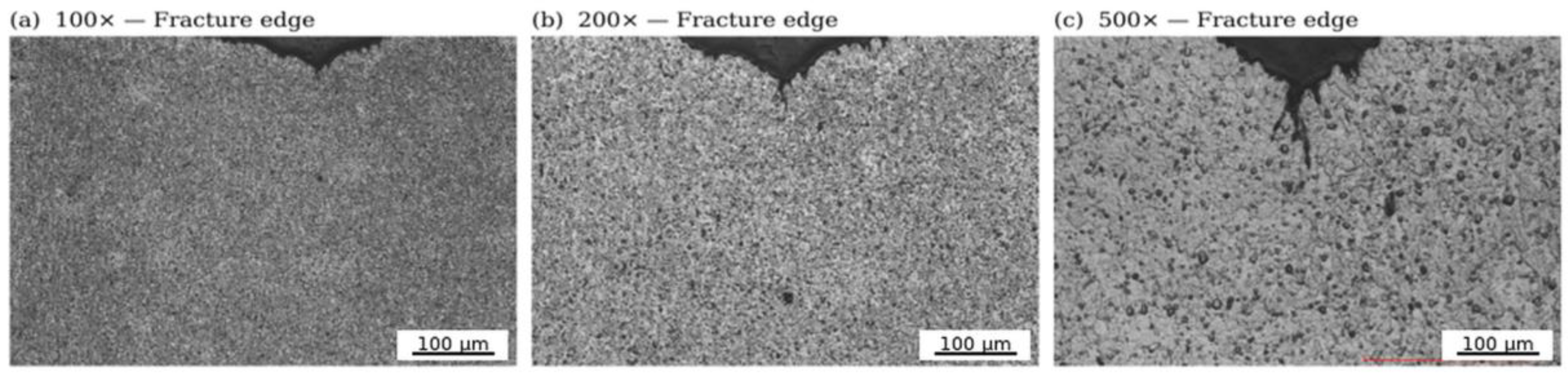
Figure 16.
Optical microstructure at the fracture edge of specimen T1 (450 °C, 10 rev s⁻¹) at increasing magnifications. Fine-grained regions adjacent to the crack surface are tentatively attributed to localized geometric DRX. Scale bars shown in all panels.
Figure 16.
Optical microstructure at the fracture edge of specimen T1 (450 °C, 10 rev s⁻¹) at increasing magnifications. Fine-grained regions adjacent to the crack surface are tentatively attributed to localized geometric DRX. Scale bars shown in all panels.
At the gauge center (Figure 17), grains are elongated parallel to the shear direction with clearly visible subgrain walls. Subgrain intercept lengths estimated from high-magnification images are approximately 5–10 μm, consistent with values reported for Al alloys undergoing DRV at comparable temperatures and strain rates [12,13]. This elongated subgrain structure, combined with the absence of large recrystallized grains, is the primary microstructural evidence for DRV at the gauge center. Quantitative confirmation via EBSD, including subgrain size distributions, LAGB fraction as a function of equivalent strain, and misorientation angle distributions, remains for future work separating DRV from cDRX contributions [15]. Once grain size d is measured by EBSD at each condition, the grain-size dependent constitutive framework σ = Aε^nε̇^m d^p exp(Q/RT) [4] can be fitted directly, enabling a process–microstructure map that links deformation parameters to grain size outcome for microstructure-controlled hot forming simulation.
The constitutive equation can also be inverted to give grain size as an explicit function of measured torque, temperature, and rotation rate: d = [T(m+3)/(2πR₀³·C⁻ᵐ·γ̇₀ᵐ·exp(mQ/RT))]¹/(ᵖᵐ), where C is a material constant and p the grain size exponent, both calibrated from EBSD-paired torsion data [4]. For closely related Al–Mg–Si specimens of identical gauge geometry, Poletti et al. [34] used EBSD and in-situ synchrotron diffraction to document the full CDRX sequence: LAGB formation begins at the specimen center at low local strain and LAGB→HAGB conversion intensifies toward the surface at high local strain, following the radial strain gradient in Section 3.1.
At the gauge edge (Figure 18), grain elongation is present but less pronounced than at the center. This radial gradient is a fundamental consequence of torsion geometry: shear strain at radius r is γ(r) = 2πNr/L, proportional to r, so the outer surface accumulates maximum shear while the specimen axis experiences none. The reported equivalent strain of 3.69 represents the outer-surface value; grain elongation and subgrain wall density decrease progressively toward the axis. Microstructure measured at any single radial position is therefore non-representative of the full cross-section, and a radially resolved EBSD study would be needed to reconstruct the full deformation history across the gauge.
8. Discussion
8.1. Comparison with the Literature
Table 7 compares the present results against prior constitutive studies on AA6061. The activation energy Q = 151.1 kJ·mol⁻¹ falls within the 142–157 kJ mol⁻¹ band reported by compression studies using α ≈ 0.040–0.045 MPa⁻¹ on the same alloy family [7,9,10]; studies employing materially different α values or temperature windows yield substantially different apparent Q (see Section 8.3). It lies 6.5% above Rokni et al. (142.8 kJ mol⁻¹ [7]), 3.6% below Citrea et al. (156.8 kJ mol⁻¹ [9]), and 1.9% above Qin et al. (148.3 kJ mol⁻¹ [10]), differences that fall comfortably within the combined experimental and regression uncertainty of ±15–25 kJ mol⁻¹ estimated in Section 5.2. This consistency across test methods and research groups confirms that Q is reproducible within the combined experimental and regression uncertainties reported by each study. The value is also consistent with Al lattice self-diffusion (142 kJ mol⁻¹ [35]), confirming that dislocation climb is the rate-controlling step for DRV in this temperature range. The present stress exponent n = 1.371 is substantially lower than compression-derived values (3.89–4.36), a systematic difference that is expected: under torsion, the flow stress at the outer surface is computed from the total torque, which integrates stress contributions from all radii, rather than from a uniform stress state. The Nadai–von Mises conversion applied here (Equation (2)) assumes m ≈ 0; a positive m would increase the inferred outer-surface stress and raise n. This geometric difference makes direct n comparisons between compression and torsion data unreliable without an m correction, and partly explains the lower n obtained here. The dominant contributor to the lower torsion n is the geometry of solid-bar torsion: the Nadai conversion integrates torque contributions from all radii weighted by r², producing a radially averaged stress response rather than a uniform surface state. This geometric averaging consistently returns lower apparent n relative to uniaxial compression for the same material [4,11]. The m ≈ 0 assumption in Equation (2) introduces an additional 2–5% underestimate of outer-surface stress for m = 0.05–0.15 (Section 3.1), which does not affect Q or relative σ_p rankings but should be noted when comparing absolute stress values with compression data.
8.2. Dynamic Recovery as Dominant Mechanism
Dynamic recovery as the dominant mechanism is supported by three independent lines of evidence. First, Q = 151.1 kJ·mol⁻¹, within 6.5% of the Al self-diffusion value (142 kJ mol⁻¹ [35]), identifies dislocation climb as the rate-limiting step, placing the dominant recovery mechanism within the climb-controlled regime expected for Al alloys across 300–550 °C [12,13]. Second, the post-peak flow stress decrease is smooth and continuous in every curve (Figure 4); the absence of abrupt drops rules out discontinuous DRX, which would produce sudden stress transients associated with rapid grain boundary migration [14]. Third, the subgrain wall network with ~5–10 μm intercept length at the gauge center (Figure 17) is characteristic of DRV microstructure [12,13]; large equiaxed recrystallized grains, which would be diagnostic of discontinuous DRX, are not observed.
At 450 °C and low strain rates, additional evidence for geometric DRX is plausible. T9 and T12 reach εmax of 5.99 and 6.36, respectively, and their flow stress curves approach an extended flat plateau rather than continuing to decline. When grain aspect ratio in torsion exceeds the critical value for geometric pinch-off (~5–10 [6,15]), geometric DRX can occur continuously and contribute to the steady state. The fine-grained zones near the fracture surface of T1 (Figure 16) are tentatively consistent with this mechanism under extreme local strains. EBSD misorientation analysis is required to confirm this attribution.
Hot torsion of AA6082, a closely related Al–Mg–Si alloy tested in specimens of identical gauge geometry (20 mm gauge, 10 mm diameter) at 350–500 °C, provides direct EBSD and synchrotron evidence for the same mechanism [34]. The flow stress plateau approaching steady state in T9 (450 °C, 0.91 s⁻¹, εₘₐₓ = 5.99) matches the CDRX-induced softening-to-steady-state transition Poletti et al. observed. Fine-grained zones near the T1 fracture surface (Figure 16) parallel the surface CDRX products documented at high local strain in AA6082. LAGB fraction versus equivalent strain profiles at multiple radial positions, and KAM maps distinguishing dislocation-dense DRV substructure from the lower-KAM signature of DRX grains, are the specific measurements required for quantitative confirmation. Until such data are acquired, the geometric DRX attribution in the present study must be treated as a microstructurally informed hypothesis rather than a confirmed mechanism.
A second-order influence on the apparent activation energy arises from the thermal stability of the strengthening precipitates during the pre-test soak. The β″ (Mg₅Si₆) needles that define the T6 temper have a metastable solvus near 250 to 300 °C and dissolve progressively above it. During the 60 to 120 s isothermal hold, specimens soaked at 300 °C retain a partially intact precipitate population, whereas those at 450 °C (T/Tₘ = 0.85) approach a near solid-solution state before deformation begins. This temperature-dependent dissolution gradient steepens the apparent flow-stress dependence on temperature between 300 and 400 °C relative to a single-phase baseline, so the reported Q = 151.1 kJ·mol⁻¹ is best interpreted as a composite apparent value that convolves climb-controlled dislocation recovery with a contribution from precipitate dissolution in the lower part of the test range. The close agreement with the Al self-diffusion energy (142 kJ·mol⁻¹) indicates that climb remains the dominant rate-controlling step, but isolating the pure-recovery activation energy would require an identical high-temperature solution treatment applied to all specimens prior to deformation.
8.3. Activation Energy and Strain-Rate Matrix Artifact
The spread in per-strain-rate Q values of 105 kJ mol⁻¹ at 0.91 s⁻¹, 158 kJ mol⁻¹ at 2.72 s⁻¹, and 194 kJ mol⁻¹ at 9.07 s⁻¹, is 89 kJ mol⁻¹ wide, far exceeding the estimated experimental uncertainty of ±15 to 25 kJ mol⁻¹. Two sources contribute, with the first dominant. First, the statistical artifact of a three-level matrix: Q at each strain rate is extracted from a three-point regression, so each slope carries large truncation error; studies with five or more strain rates consistently report tighter Q bands [9,19]. Second, adiabatic heating at 9.07 s⁻¹ (Section 5.3): the effective temperature at peak stress may be 7–12 °C above the nominal target, which systematically raises the inferred slope in the ln[sinh(ασp)]–1000/T regression and inflates the high-rate Q. The global mean Q = 151.1 kJ·mol⁻¹ averages across both artifacts and is considered physically representative of climb-controlled dislocation motion in this alloy.
Prasad and Seshacharyulu document that apparent Q and n derived from kinetic rate equations are inherently range-dependent when the test window spans multiple deformation mechanism regimes [33]. The 89 kJ mol⁻¹ spread in per-strain-rate Q observed here reflects both that phenomenon and the statistical and adiabatic sources identified above. Any single per-rate Q value is therefore unreliable as a mechanism diagnostic without independent microstructural verification.
To quantify the contribution of uncompensated adiabatic heating to the per-rate Q spread, the sequential three-point regression at 9.07 s⁻¹ was repeated substituting T_(eff) from Table 5 in place of the nominal temperatures. The T_(eff) values for the three 9.07 s⁻¹ conditions are 735, 680, and 631 K for the nominal 450, 400, and 350 °C targets. The slope d(ln[sinh(ασ_p)])/d(1/T) changes from 6,997 K (nominal) to 6,887 K (corrected), a reduction of 1.6%. Scaled to the reported per-rate Q of 194 kJ mol⁻¹ at 9.07 s⁻¹, the adiabatic correction reduces this value by approximately 3 kJ mol⁻¹ (194 → 191 kJ mol⁻¹). This represents 3% of the 89 kJ mol⁻¹ per-rate spread and falls within the stated experimental uncertainty of ±15–25 kJ mol⁻¹. The adiabatic contribution is therefore negligible; the dominant source of the spread is the statistical limitation of three-point per-rate regressions. The global mean Q = 151.1 kJ mol⁻¹ averages across all three strain rates and remains the most reliable estimate of the apparent activation energy, insensitive to the adiabatic correction.
8.4. Model Accuracy and Scope of Application
The training AARE of 15.5% and LOO-CV AARE of 23.0% exceed the 5–10% typical of wider compression datasets [7,9]. These elevated errors reflect the compounding of three factors already quantified: the 24% T1–T6 repeatability noise (Section 4.5), systematic adiabatic bias at 9.07 s⁻¹ (Section 5.3), and limited leverage at matrix corners (Section 5.5.2). These three sources together set a practical accuracy ceiling of approximately 15% for constitutive models calibrated on this dataset. For process simulation, this translates to a σ uncertainty of roughly ±10–15 MPa across the 45–110 MPa range of the hot-working regime, which is acceptable for initial die design and process window selection but insufficient for fatigue-critical applications. Expanding to at least five strain rates per temperature across three decades, repeating two or three conditions, and digitizing full torque–rotation records would each independently narrow the uncertainty band.
From a process engineering standpoint, the ±10–15 MPa flow stress uncertainty from this dataset translates directly to force and pressure prediction uncertainty in hot forming simulation. For a typical AA6061 extrusion die operating at 400–450 °C and 1–10 s⁻¹ equivalent strain rate, a 15% AARE in constitutive prediction corresponds to approximately 7–16 MPa variation in predicted ram pressure at fixed die geometry. This is acceptable for preliminary die design and process window selection, where a 10–20% safety margin is routinely applied, but insufficient for fatigue-critical tooling qualification or spring-back prediction in sheet forming. The practical implication for process engineers is that the present dataset and constitutive equation are reliable for identifying the safe forming window (400–450 °C, 0.91–2.72 s⁻¹), for excluding 350 °C as an unstable operating condition, and for FE-based die filling and load estimation at the feasibility stage. Tighter predictions for final tooling design require a conditioning matrix of at least five temperatures and five strain rates with replicated conditions.
A data-driven alternative requires no additional experiments. For AA6061 at 375–575 °C, Ding et al. [36] showed that a two-hidden-layer artificial neural network trained on Gleeble compression data achieved RMSE = 1.68 MPa, half the 3.43 MPa of the Sellars–Tegart equation. Applied to the present torsion dataset, a comparably compact ANN would require no fixed α and would capture non-Arrhenius behavior at matrix corners, reducing LOO-CV errors at T9 and T7.
8.5. Processing Map and Industrial Relevance
The processing map (Figure 13) identifies two distinct regimes. The instability region at 350 °C corresponds to conditions where m is negative (flow stress decreases with increasing strain rate), meaning that any local perturbation in strain rate amplifies rather than dissipates, leading to adiabatic shear banding and fracture. This prediction is fully confirmed by direct macroscopic observation of fracture in all three specimens at 350 °C. The stable high-η window at 400–450 °C and 0.91–2.72 s⁻¹ corresponds to conditions where DRV efficiently dissipates stored energy and produces uniform microstructure. These conditions align well with industrial AA6061 extrusion practice (400–480 °C, exit speed equivalent to 1–5 s⁻¹ equivalent strain rate), providing independent validation of the map from industrial experience.
The instability criterion ξ < 0 has a physical basis: it identifies conditions where the material cannot generate entropy at the rate imposed by deformation, so flow localizes rather than distributes uniformly [33]. At 350 °C, ξ decreases from −0.19 at 0.91 s⁻¹ to −0.86 at 9.07 s⁻¹, reflecting the progressive inability of DRV to accommodate rising dislocation generation rates. Every specimen tested at 350 °C fractured, confirming the prediction.
9. Conclusions
1. Gleeble hot torsion of AA6061-T6 from 250 to 450 °C and 0.91 to 9.07 s⁻¹ produced flow curves with three-stage behavior: work hardening, dynamic softening, and quasi-steady state, consistent across all eleven conditions. Peak flow stress ranges from 44.8 to 219.9 MPa. Temperature sensitivity steepens below ~300 °C, consistent with a transition from climb-limited to glide-limited deformation.
2. One-step Levenberg–Marquardt nonlinear regression of ε̇ = A exp(−Q/RT) [sinh(ασp)]n over all ten hot-working conditions simultaneously yields Q = 151.1 kJ·mol⁻¹, n = 1.371, A = 3.51 × 10¹⁰ s⁻¹, and α = 0.045 MPa⁻¹. Training accuracy is AARE = 15.5%, RMSE = 13.6 MPa, R = 0.908; LOO-CV gives AARE = 23.0%, bounding the predictive uncertainty. The parallel fit using local fracture-site strain rates agrees within 4% on Q, confirming that gauge non-uniformity does not significantly affect Q at this specimen scale.
3. The per-strain-rate Q spread (105–194 kJ mol⁻¹) reflects two compounding factors: the statistical artifact of a three-level strain-rate matrix (dominant source, accounting for ∼97% of the spread per the adiabatic-corrected regression in Section 8.3) and uncompensated adiabatic heating at 9.07 s⁻¹ (estimated ΔT_(ad) ≤ 12.3 °C, contributing ≤3 kJ mol⁻¹). The global mean Q is representative and consistent with Al lattice self-diffusion.
4. The Prasad instability map identifies 400–450 °C at 0.91–2.72 s⁻¹ as the preliminary optimal hot-forming window (η = 0.35–0.48). Flow instability predicted at 350 °C is confirmed by macroscopic fracture in every specimen tested there. The 3 × 3 grid provides directional guidance; a high-fidelity map requires at least five strain rates and five temperatures.
5. Repeatability testing (T1 vs. T6 at 450 °C/10 rev s⁻¹) revealed a 24% peak stress discrepancy, attributed to thermocouple attachment variability [28] and differences in strain localization. This scatter has been explicitly propagated into the model uncertainty as ±15 to 25 kJ mol⁻¹ on Q and sets a practical noise floor of ~15% AARE for constitutive models calibrated on this dataset.
6. Optical microscopy of specimen T1 at four locations establishes dynamic recovery as the dominant restoration mechanism: Q ≈ Al self-diffusion, gradual post-peak softening without abrupt stress drops, and elongated grains with ~5–10 μm subgrain walls at the gauge center (Figure 17). Fine-grained zones near the fracture surface (Figure 16) are tentatively attributed to localized geometric DRX under extreme crack-tip strain concentration. EBSD misorientation analysis, LAGB fraction quantification, and KAM mapping are required to definitively resolve the DRV–DRX boundary.
7. A preliminary strain-compensated Arrhenius framework is reported through fifth-order polynomial fits to n(ε), Q(ε), and ln(A(ε)) (Equations (8)–(10), Table 6), derived using a literature-based flow-curve shape function (Equation (7)) because digitized torque–rotation records were unavailable at submission. The fits are reliable only for ε ≥ 0.8 (R² = 0.83–0.85); the transient regime ε < 0.8 carries R² = 0.36–0.40 and must not be used in simulation. This framework is therefore a starting point requiring validation against directly measured flow curves before any production FE use, and is not presented as a calibrated FE-ready model.
8. The Nadai–von Mises conversion in Equation (2) carries a 2–5% systematic underestimate of outer-surface flow stress from the m ≈ 0 assumption (Section 3.1); this does not affect Q or relative σ_p rankings. The lower apparent n relative to compression datasets reflects the radial stress-averaging geometry of solid-bar torsion (Section 8.1); direct n comparisons across test methods require a radial correction.
Supplementary Materials
The following supporting information can be downloaded at the website of this paper posted on Preprints.org.
Author Contributions
Conceptualization, X.W.; methodology, A.N.E.; investigation, A.N.E.; formal analysis, A.N.E.; data curation, A.N.E.; writing of the original draft, A.N.E.; review and editing of the manuscript, H.A.; review and editing of the manuscript.; supervision, X.W.; resources, All authors have read and agreed to the published version of the manuscript.
Funding
This research received no external funding.
Data Availability Statement
The raw torque–rotation data, the reduced flow stress–strain curves, and the Python regression scripts generated and analyzed in this study are available from the corresponding author upon reasonable request.
Acknowledgments
The authors acknowledge access to the Gleeble Hot Torsion facility at Dynamic Systems Inc. (Poestenkill, NY, USA) and the metallographic and microscopy support provided at Wayne State University.
Conflicts of Interest
The authors declare no conflicts of interest.
References
- J. Davis, Aluminum and Aluminum Alloys, ASM International, Materials Park, OH, 1993.
- I.J. Polmear, Light Alloys: From Traditional Alloys to Nanocrystals, 4th ed., Elsevier/Butterworth-Heinemann, Oxford, 2006.
- W.F. Hosford, R.M. Caddell, Metal Forming: Mechanics and Metallurgy, 4th ed., Cambridge University Press, Cambridge, 2011.
- H.J. McQueen, J.J. Jonas, Hot workability testing techniques, in: Treatise on Materials Science and Technology, vol. 6, Academic Press, New York, 1975, pp. 393–493.
- S.L. Semiatin, J.H. Holbrook, Plastic flow phenomenology of 304L stainless steel, Metallurgical Transactions A 14 (1983) 1681–1695. [CrossRef]
- K.T. Son, C.H. Cho, M.G. Kim, Two-stage dynamic recrystallization and texture evolution in Al-7Mg alloy during hot torsion, International Journal of Minerals, Metallurgy and Materials 31 (2024) 1900–1911. [CrossRef]
- M. Rokni, A. Zarei-Hanzaki, A.A. Roostaei, H.R. Abedi, An investigation into the hot deformation characteristics of 6061 aluminum alloy, Materials and Design 32 (2011) 2339–2344. [CrossRef]
- H.R. Ezatpour, M. Haddad Sabzevar, S.A. Sajjadi, Y. Huang, Investigation of work softening mechanisms and texture in a hot deformed 6061 aluminum alloy at high temperature, Materials Science and Engineering A 606 (2014) 240–247. [CrossRef]
- T. Citrea, A.E. Tekkaya, S. Siemer, Constitutive modelling of the 6061 aluminium alloy under hot rolling conditions and large strain ranges, Materials and Design 191 (2020) 108639. [CrossRef]
- F. Qin, H. Qi, Y. Li, A comparative study of constitutive characteristics and microstructure evolution between uniaxial and plane strain compression of an AA6061 alloy, Journal of Materials Engineering and Performance 28 (2019) 3487–3497. [CrossRef]
- H.J. McQueen, S. Spigarelli, M.E. Kassner, E. Evangelista, Hot Deformation and Processing of Aluminum Alloys, CRC Press, Boca Raton, FL, 2011.
- X.H. Fan, M. Li, D.Y. Li, Y.C. Shao, S.R. Zhang, Y.H. Peng, Dynamic recrystallisation and dynamic precipitation in AA6061 aluminium alloy during hot deformation, Materials Science and Technology 30 (2014) 1263–1272. [CrossRef]
- A. Chamanfar, M.T. Alamoudi, N.E. Nanninga, W.Z. Misiolek, Analysis of flow stress and microstructure during hot compression of 6099 aluminum alloy (AA6099), Materials Science and Engineering A 743 (2019) 684–696. [CrossRef]
- K. Huang, R.E. Logé, A review of dynamic recrystallization phenomena in metallic materials, Materials and Design 111 (2016) 548–574. [CrossRef]
- S.J. Zheng, X.H. Yuan, X. Gong, T. Le, A.V. Ravindra, Mechanistic insights and kinetics of continuous and geometric dynamic recrystallisation in hot deformed aluminium alloy, Acta Materialia 283 (2025) 120534. [CrossRef]
- F. Garofalo, An empirical relation defining the stress dependence of minimum creep rate in metals, Transactions of the Metallurgical Society of AIME 227 (1963) 351–356.
- C. Zener, J.H. Hollomon, Effect of strain rate upon plastic flow of steel, Journal of Applied Physics 15 (1944) 22–32. [CrossRef]
- H. Li, C. Zhu, S. Li, H. Jiang, P. Zhang, R. Yang, S. Zhao, A modified Johnson–Cook model for modeling AA6061-T6 under different temperatures considering ductile fracture, Journal of Materials Engineering and Performance 33 (2024) 1047–1061. [CrossRef]
- T. Citrea, A.E. Tekkaya, Comparison study of constitutive models in predicting the hot deformation behavior of AA6060 and AA6063 aluminium alloys, Materials Today: Proceedings 87 (2023) 351–355. [CrossRef]
- H.J. McQueen, E. Evangelista, N.D. Ryan, Restoration mechanisms in Al alloys and their hot torsion test determination, in: T.R. McNelley (Ed.), Recrystallization ’96, TMS, Warrendale, PA, 1997, pp. 365–376.
- Dynamic Systems Inc., Hot Torsion Testing on a Gleeble System, Application Note APN020, DSI, Poestenkill, NY, 2017.
- S.L. Semiatin, D.W. Mahaffey, N.C. Levkulich, O.N. Senkov, The radial temperature gradient in the Gleeble hot-torsion test and its effect on the interpretation of plastic-flow behavior, Metallurgical and Materials Transactions A 48 (2017) 5357–5372. [CrossRef]
- D.R. Forrest, M.F. Sinfield, Numerical Simulation of Gleeble Torsion Testing of HSLA-65 Steel, Report NSWCCD-61-TR-2008/02, Naval Surface Warfare Center Carderock Division, 2008.
- C.M. Sellars, W.J. McTegart, On the mechanism of hot deformation, Acta Metallurgica 14 (1966) 1136–1138. [CrossRef]
- Y.V.R.K. Prasad, H.L. Gegel, S.M. Doraivelu, J.C. Malas, J.T. Morgan, K.A. Lark, D.R. Barker, Modeling of dynamic material behavior in hot deformation: forging of Ti-6242, Metallurgical Transactions A 15 (1984) 1883–1892. [CrossRef]
- Y.V.R.K. Prasad, S. Sasidhara, Hot Working Guide: A Compendium of Processing Maps, ASM International, Materials Park, OH, 1997.
- Z. Chen, G. Fang, J. Zhao, Formability evaluation of aluminum alloy 6061-T6 sheet at room and elevated temperatures, Journal of Materials Engineering and Performance 26 (2017) 4626–4637. [CrossRef]
- Dynamic Systems Inc., Thermocouple Attachment Techniques for Dynamic Thermocouple Measurements, Application Note APN026, DSI, Poestenkill, NY, 2017.
- Dynamic Systems Inc., Diffusion Effects on Type K (Cr-Al) Thermocouple Measurements, Application Note APN010, DSI, Poestenkill, NY, 2017.
- H.J. McQueen, N.D. Ryan, Constitutive analysis in hot working, Materials Science and Engineering A 322 (2002) 43–63. [CrossRef]
- I. Farup, J.-M. Drezet, A. Mo, T. Iveland, Gleeble machine determination of creep law parameters for thermally induced deformations in aluminium DC casting, Journal of Thermal Stresses 23 (2000) 47–58. [CrossRef]
- H. Shi, A.J. McLaren, C.M. Sellars, R. Shahani, R. Bolingbroke, Constitutive equations for high temperature flow stress of aluminium alloys, Materials Science and Technology 13 (1997) 210–216. [CrossRef]
- Y.V.R.K. Prasad, T. Seshacharyulu, Modelling of hot deformation for microstructural control, International Materials Reviews 43 (1998) 243–258. [CrossRef]
- M.C. Poletti, T. Simonet-Fotso, D. Halici, D. Canelo-Yubero, F. Montheillet, D. Piot, Z. Kovács, N. Schell, D. Tolnai, Continuous dynamic recrystallization during hot torsion of an aluminum alloy, Journal of Physics: Conference Series 1270 (2019) 012049. [CrossRef]
- T. Perälä, P. Taskinen, Diffusion data for binary aluminum alloys, Scandinavian Journal of Metallurgy 29 (2000) 162–169. [CrossRef]
- S. Ding, Q. Shi, G. Chen, Flow stress of 6061 aluminum alloy at typical temperatures during friction stir welding based on hot compression tests, Metals 11 (2021) 804. [CrossRef]
Figure 1.
Simplified schematic of the AA6061-T6 solid-bar torsion specimen with critical dimensions labeled.
Figure 1.
Simplified schematic of the AA6061-T6 solid-bar torsion specimen with critical dimensions labeled.
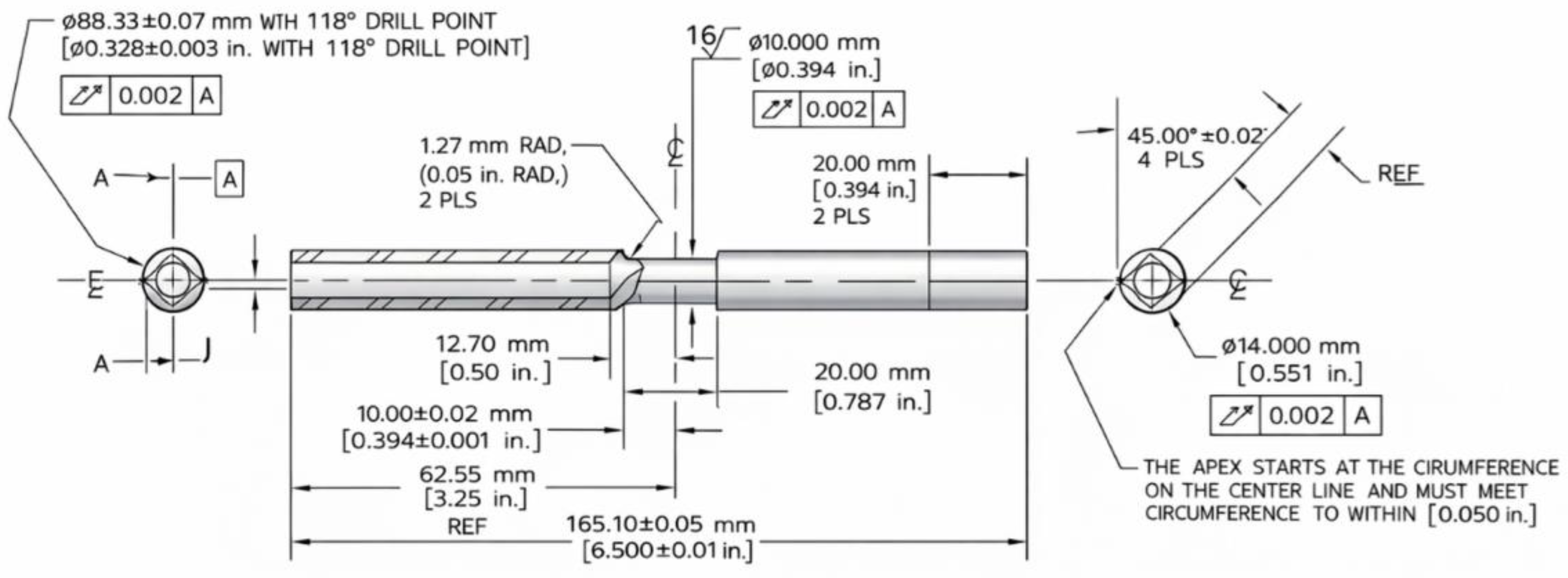
Figure 2.
AA6061-T6 torsion specimen with axial reference line scribed on the gauge surface prior to testing.
Figure 2.
AA6061-T6 torsion specimen with axial reference line scribed on the gauge surface prior to testing.

Figure 3.
Epoxy-mounted axial cross-sections: (a) AA6061-T6 as-received; (b) post-deformation specimen T1 (450 °C, 10 rev s⁻¹). Scale bar = 5 mm.
Figure 3.
Epoxy-mounted axial cross-sections: (a) AA6061-T6 as-received; (b) post-deformation specimen T1 (450 °C, 10 rev s⁻¹). Scale bar = 5 mm.
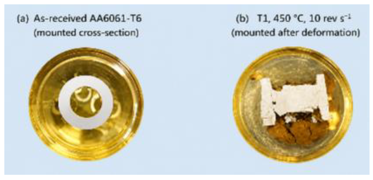
Figure 4.
Equivalent flow stress versus equivalent strain for AA6061-T6 at all eleven conditions, grouped by equivalent strain rate. Filled circles mark the peak stress on each curve.
Figure 4.
Equivalent flow stress versus equivalent strain for AA6061-T6 at all eleven conditions, grouped by equivalent strain rate. Filled circles mark the peak stress on each curve.
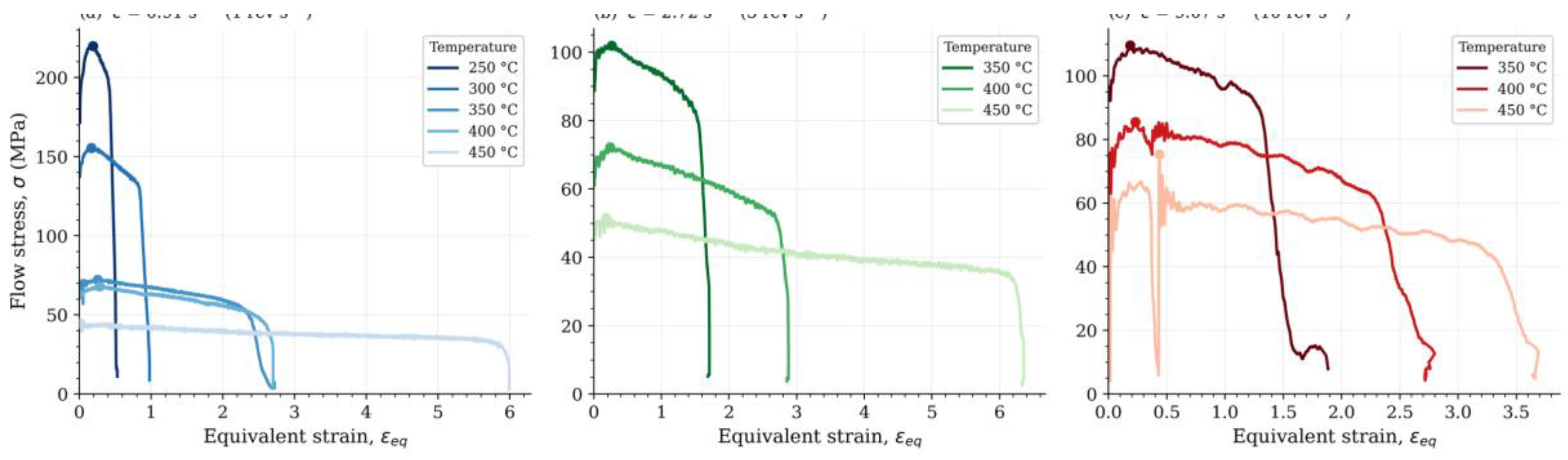
Figure 5.
Peak flow stress as a function of (a) deformation temperature at three equivalent strain rates, and (b) equivalent strain rate at four deformation temperatures.
Figure 5.
Peak flow stress as a function of (a) deformation temperature at three equivalent strain rates, and (b) equivalent strain rate at four deformation temperatures.
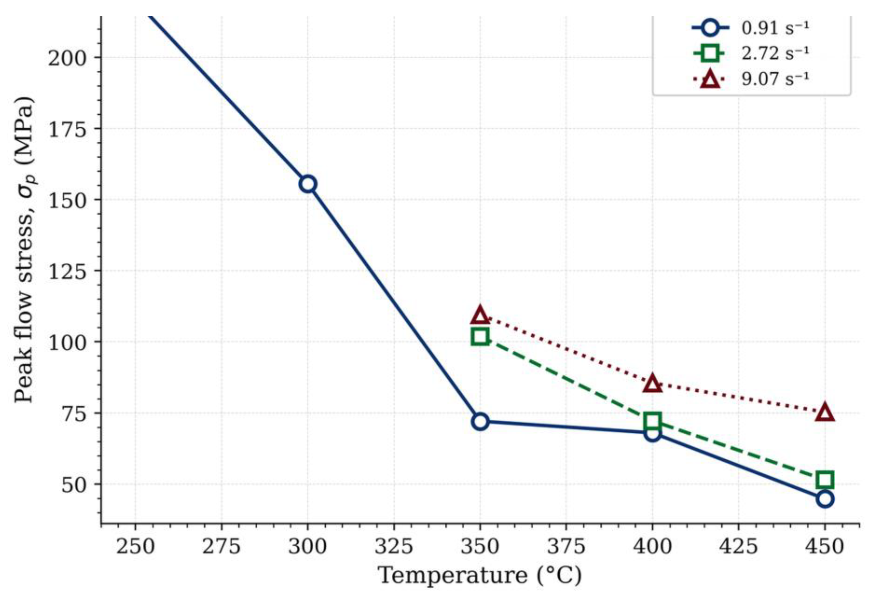
Figure 6.
(a) Maximum equivalent strain and (b) peak flow stress versus rotation rate (rev s⁻¹, log scale) for each test temperature. Panels are aligned vertically for direct comparison.
Figure 6.
(a) Maximum equivalent strain and (b) peak flow stress versus rotation rate (rev s⁻¹, log scale) for each test temperature. Panels are aligned vertically for direct comparison.
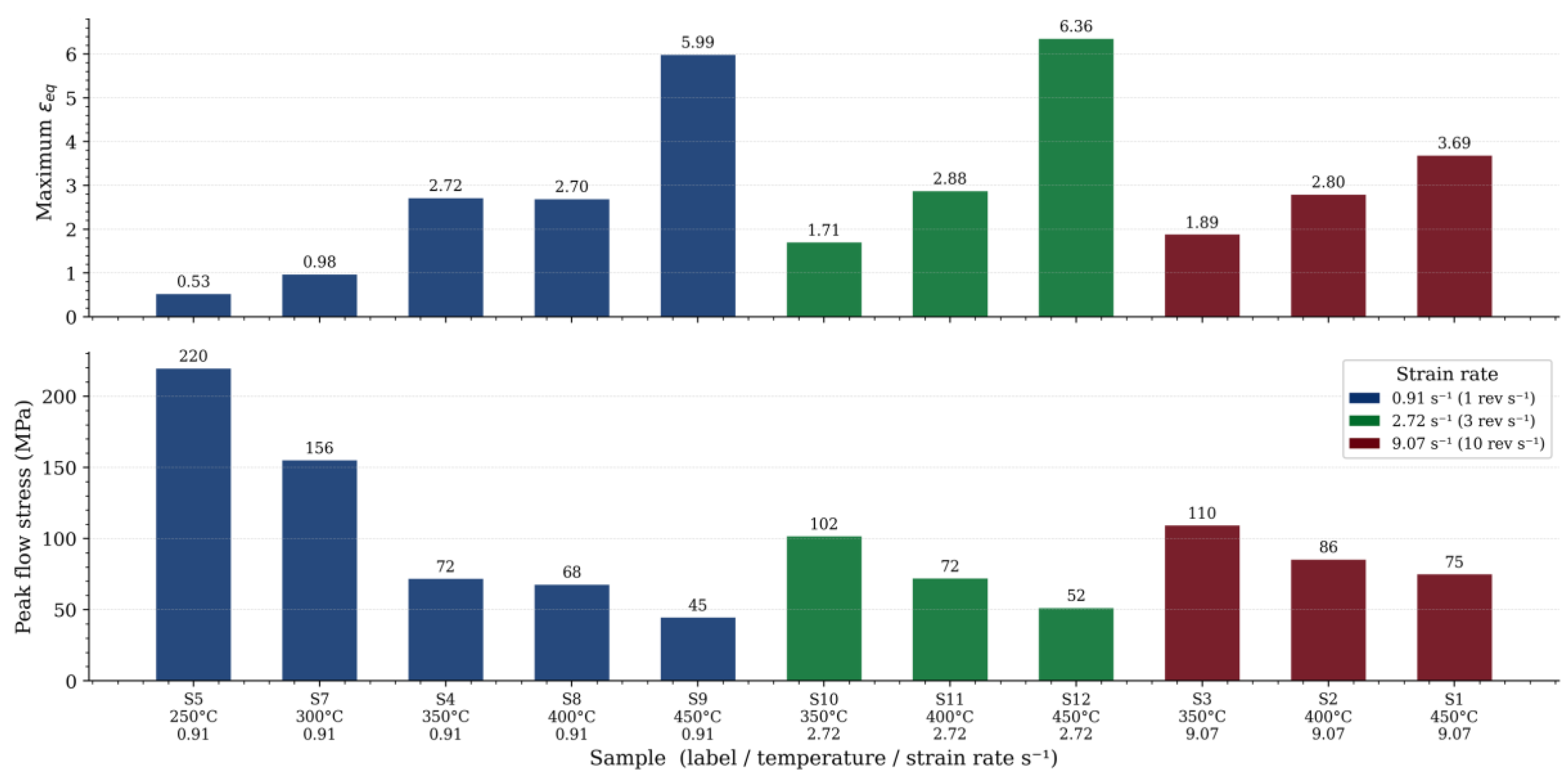
Figure 7.
Post-deformation macroscopic appearance: (a) T1 (450 °C/10 rev s⁻¹), T2 (400 °C/10), T3 (350 °C/10), and T9 (450 °C/1 rev s⁻¹); (b) T12 (450 °C/3 rev s⁻¹) showing a circumferential crack across approximately 3/4 of the gauge diameter.
Figure 7.
Post-deformation macroscopic appearance: (a) T1 (450 °C/10 rev s⁻¹), T2 (400 °C/10), T3 (350 °C/10), and T9 (450 °C/1 rev s⁻¹); (b) T12 (450 °C/3 rev s⁻¹) showing a circumferential crack across approximately 3/4 of the gauge diameter.
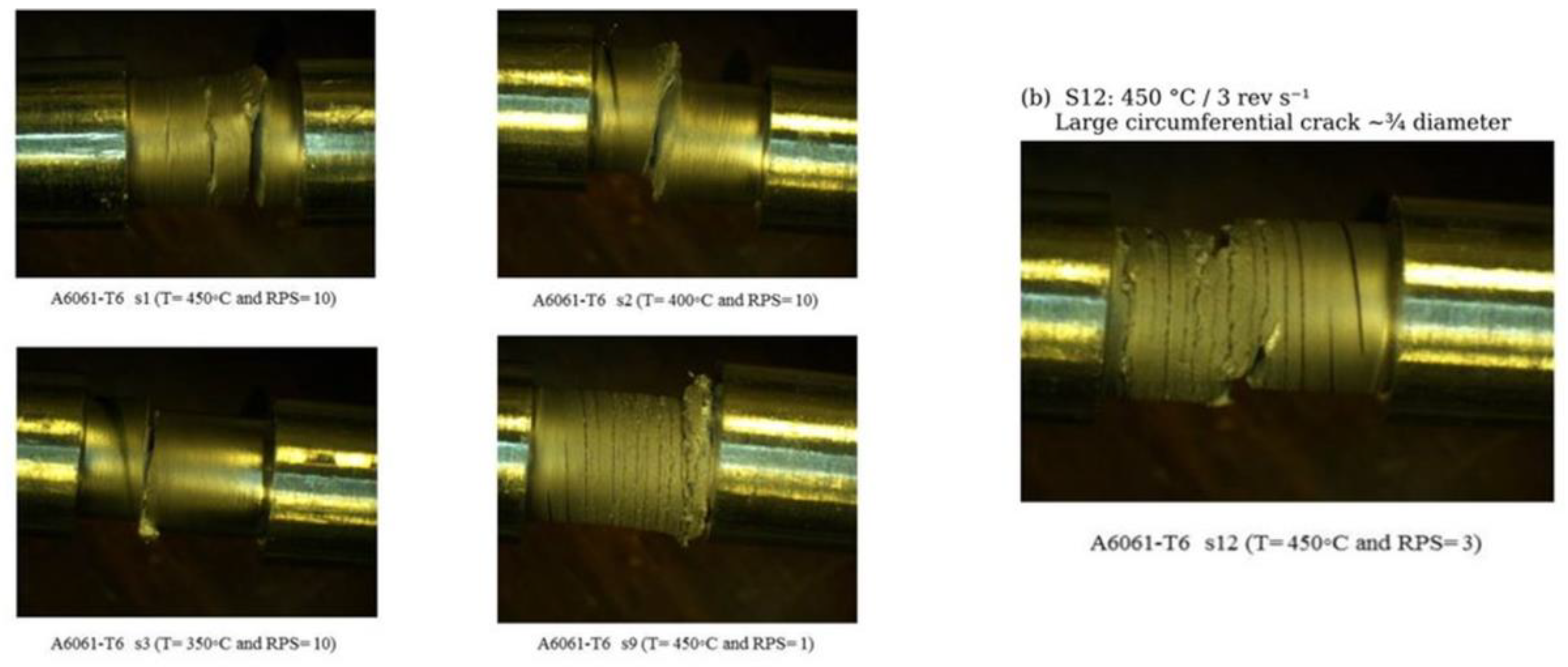
Figure 8.
Flow curves for specimens T1 and T6 (both 450 °C, 10 rev s⁻¹). Filled circles mark peak stress. The 24% peak stress difference reflects thermocouple attachment variability and strain localization.
Figure 8.
Flow curves for specimens T1 and T6 (both 450 °C, 10 rev s⁻¹). Filled circles mark peak stress. The 24% peak stress difference reflects thermocouple attachment variability and strain localization.
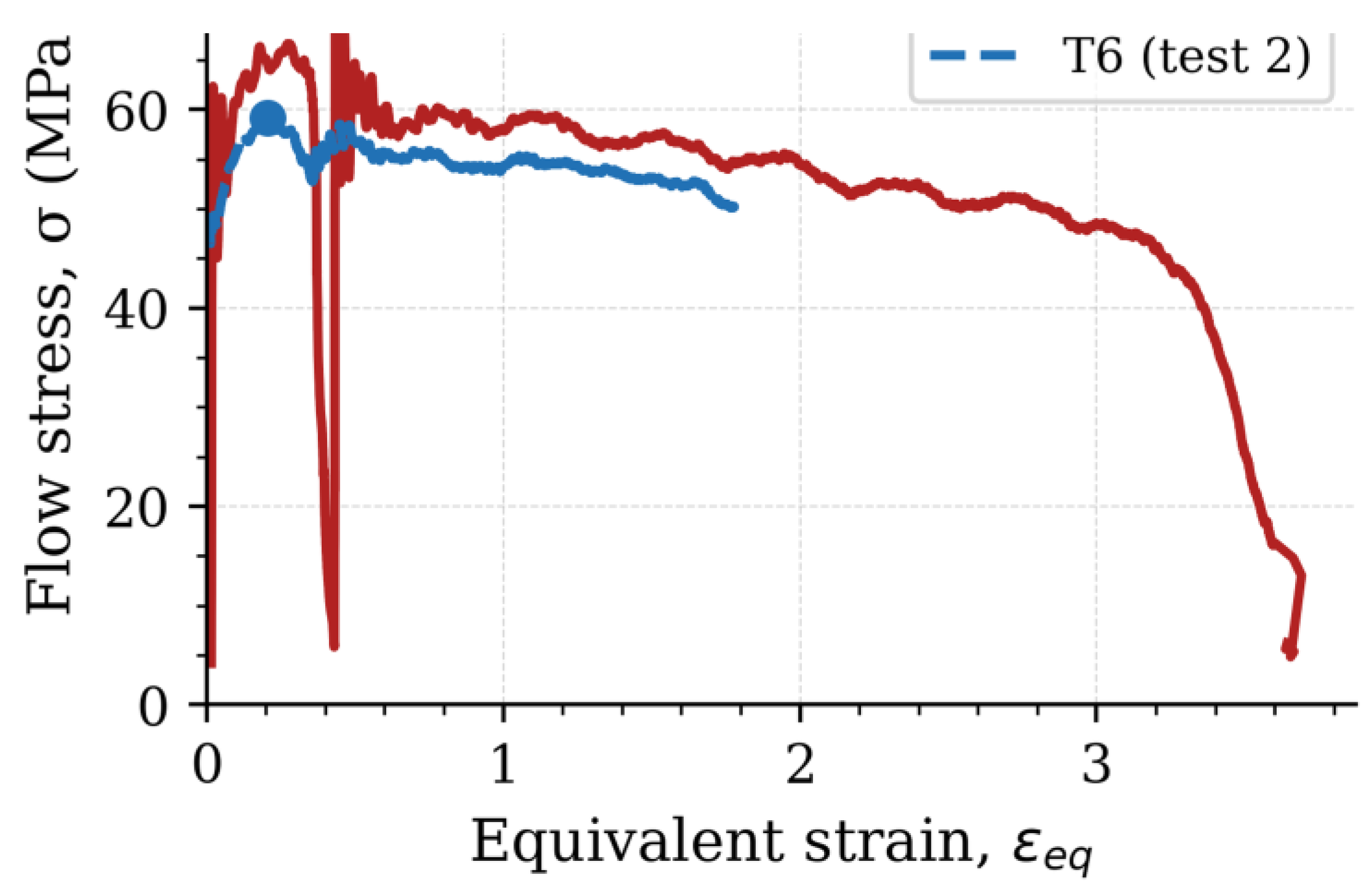
Figure 9.
ln(ε̇) versus ln[sinh(ασ_p)] at three temperatures for determination of stress exponent n (α = 0.045 MPa⁻¹). Points from the one-step fit shown for reference.
Figure 9.
ln(ε̇) versus ln[sinh(ασ_p)] at three temperatures for determination of stress exponent n (α = 0.045 MPa⁻¹). Points from the one-step fit shown for reference.
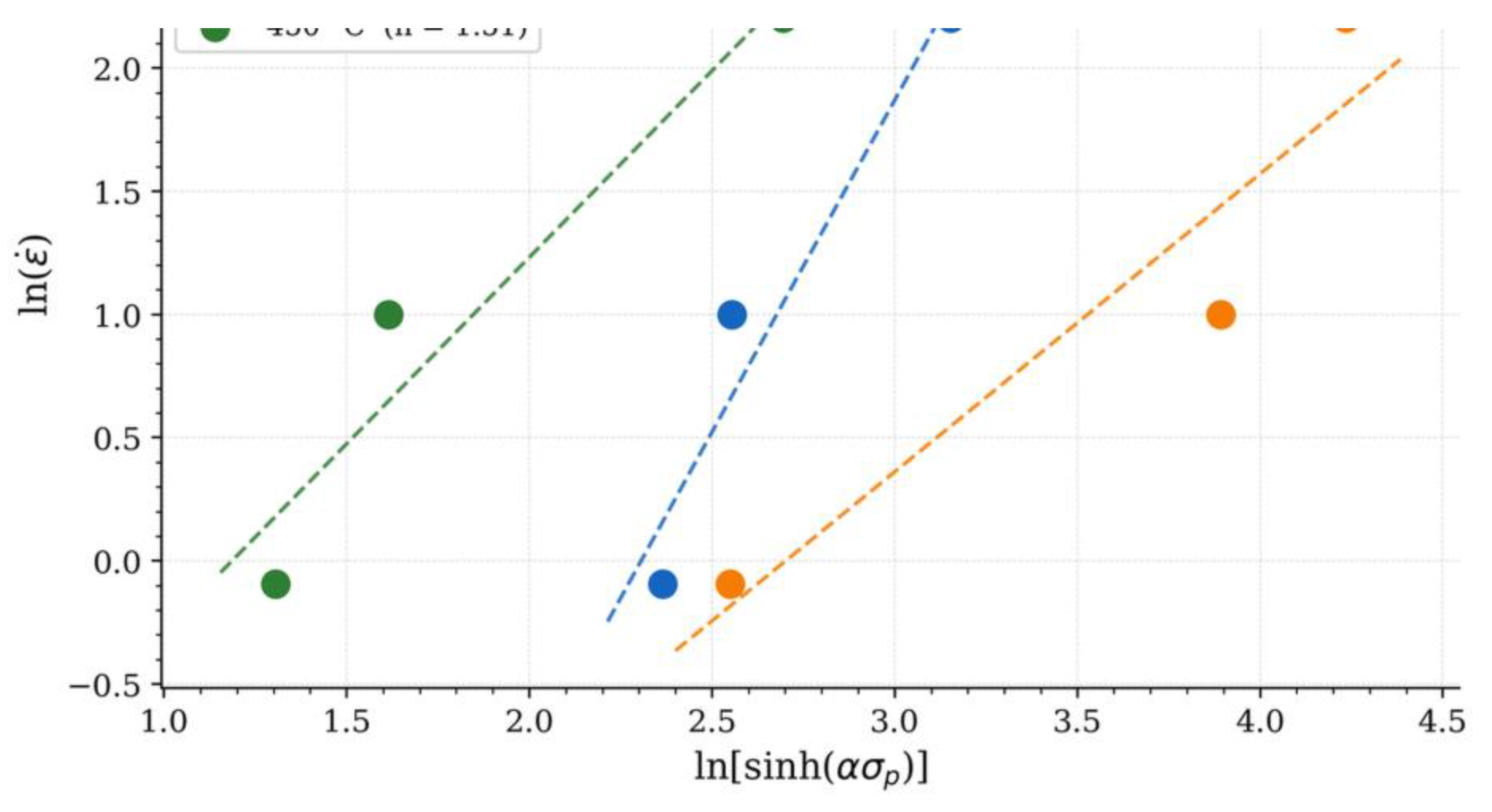
Figure 10.
ln[sinh(ασ_p)] versus 1000/T at three strain rates for determination of apparent activation energy Q.
Figure 10.
ln[sinh(ασ_p)] versus 1000/T at three strain rates for determination of apparent activation energy Q.
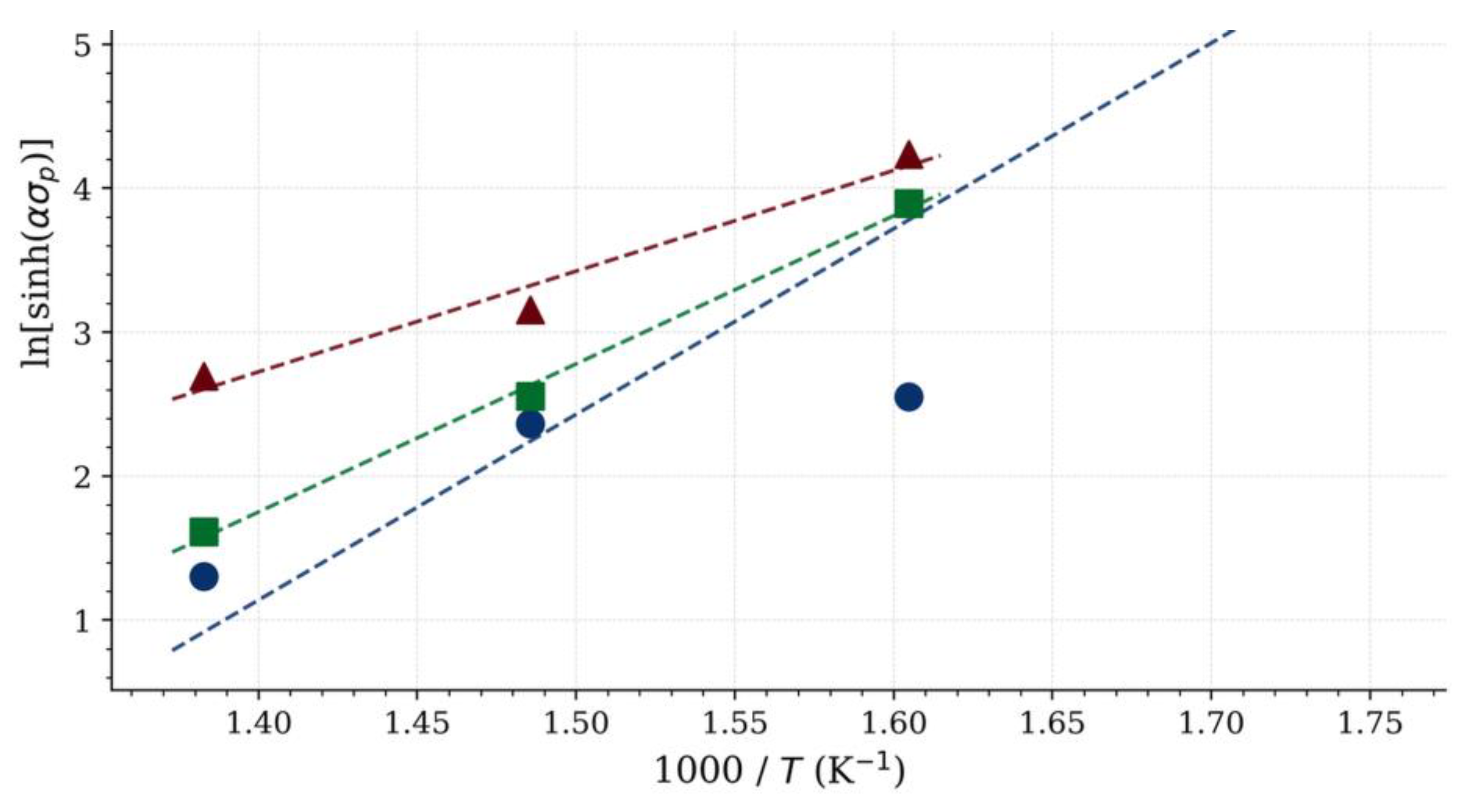
Figure 11.
Global Zener–Hollomon correlation: ln(Z) versus ln[sinh(ασ_p)] for all ten hot-working conditions (300–450 °C).
Figure 11.
Global Zener–Hollomon correlation: ln(Z) versus ln[sinh(ασ_p)] for all ten hot-working conditions (300–450 °C).
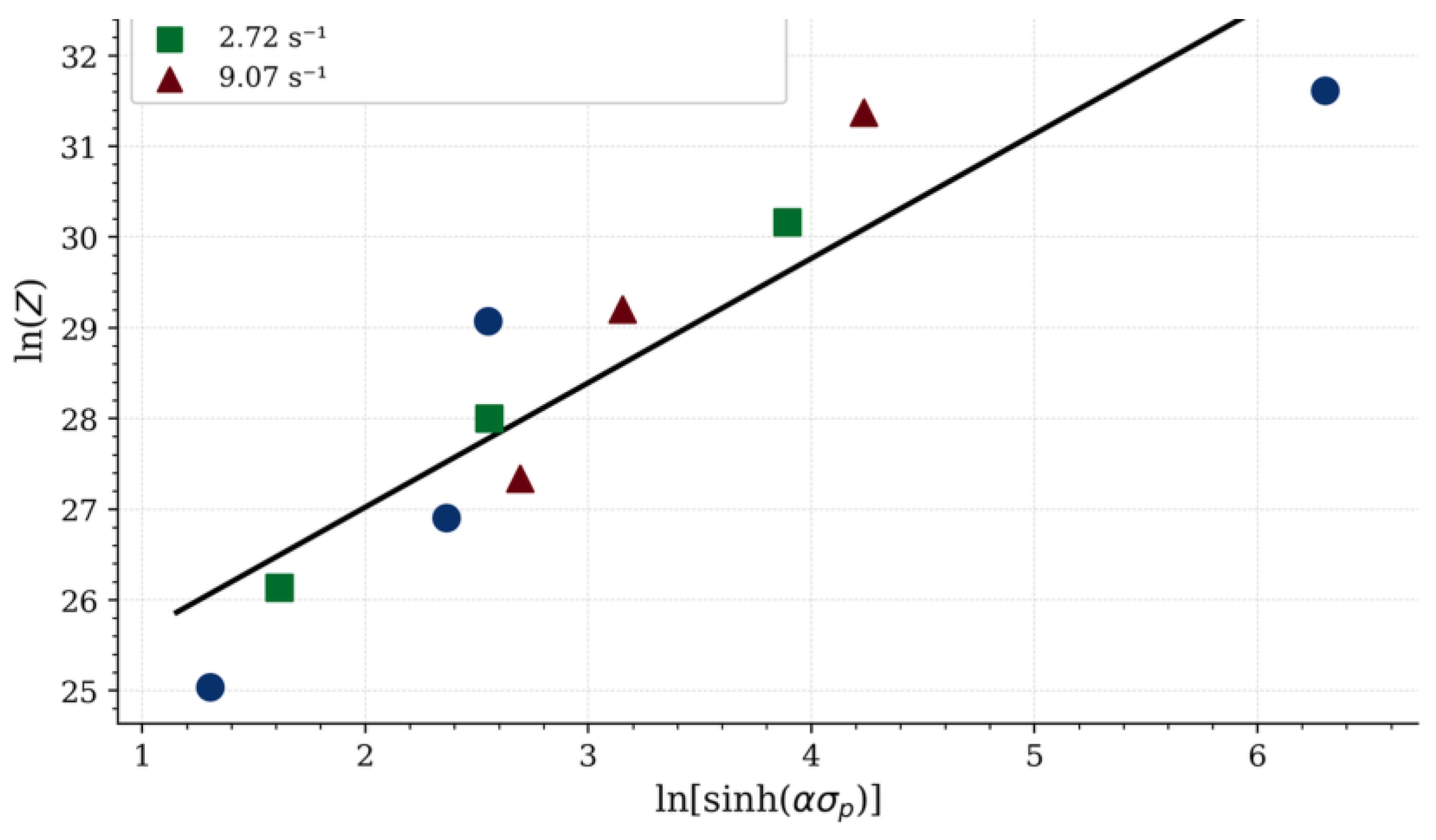
Figure 12.
Predicted versus experimental peak flow stress for AA6061-T6 (ten hot-working conditions, 300–450 °C). Dashed line: perfect agreement; gray band: ±10% error. AARE = 15.5%, RMSE = 13.6 MPa, R = 0.908.
Figure 12.
Predicted versus experimental peak flow stress for AA6061-T6 (ten hot-working conditions, 300–450 °C). Dashed line: perfect agreement; gray band: ±10% error. AARE = 15.5%, RMSE = 13.6 MPa, R = 0.908.
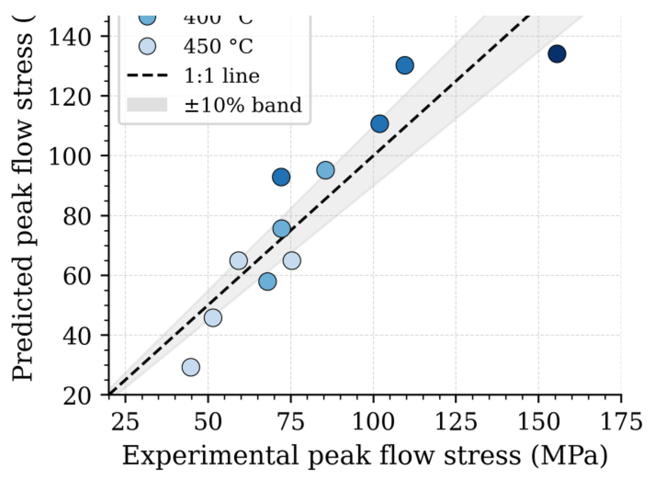
Figure 14.
Optical microstructure of AA6061-T6 as-received at three magnifications. Scale bars shown in each panel.
Figure 14.
Optical microstructure of AA6061-T6 as-received at three magnifications. Scale bars shown in each panel.
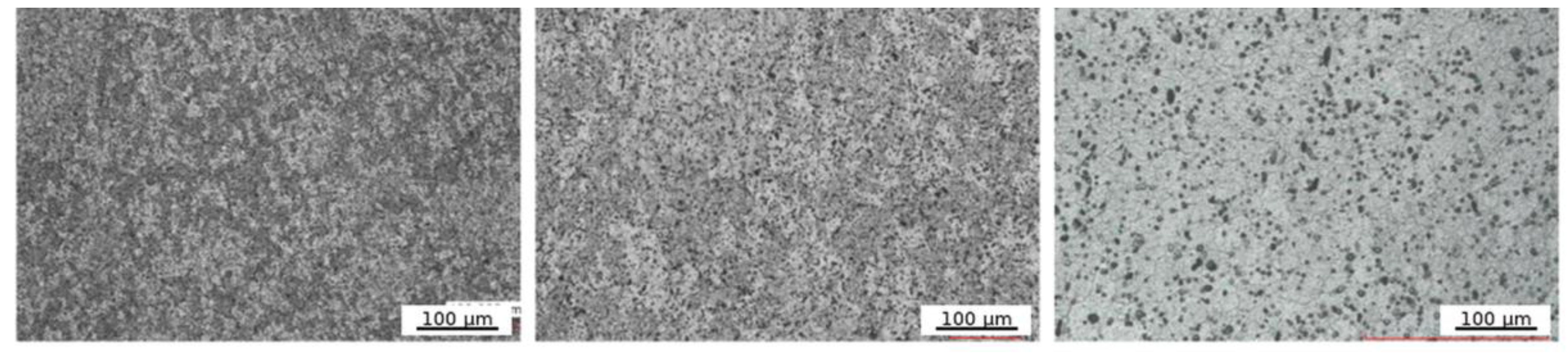
Figure 15.
Optical microstructure at the gauge–shoulder boundary of specimen T1 (450 °C, 10 rev s⁻¹) at increasing magnifications. Scale bars shown in all panels.
Figure 15.
Optical microstructure at the gauge–shoulder boundary of specimen T1 (450 °C, 10 rev s⁻¹) at increasing magnifications. Scale bars shown in all panels.
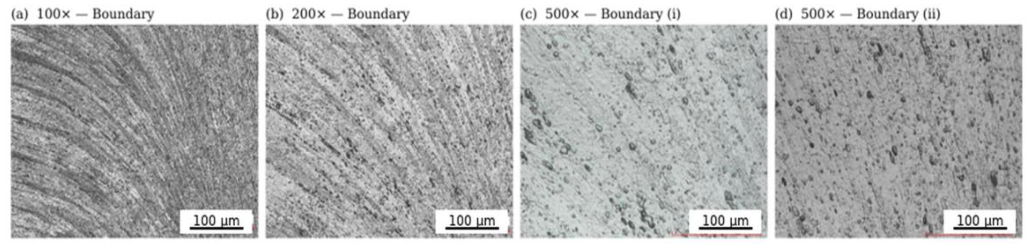
Figure 17.
Optical microstructure at the gauge center of specimen T1 (450 °C, 10 rev s⁻¹). Elongated grains with subgrain walls ~5–10 μm in intercept length are consistent with dynamic recovery. Scale bars shown in all panels.
Figure 17.
Optical microstructure at the gauge center of specimen T1 (450 °C, 10 rev s⁻¹). Elongated grains with subgrain walls ~5–10 μm in intercept length are consistent with dynamic recovery. Scale bars shown in all panels.
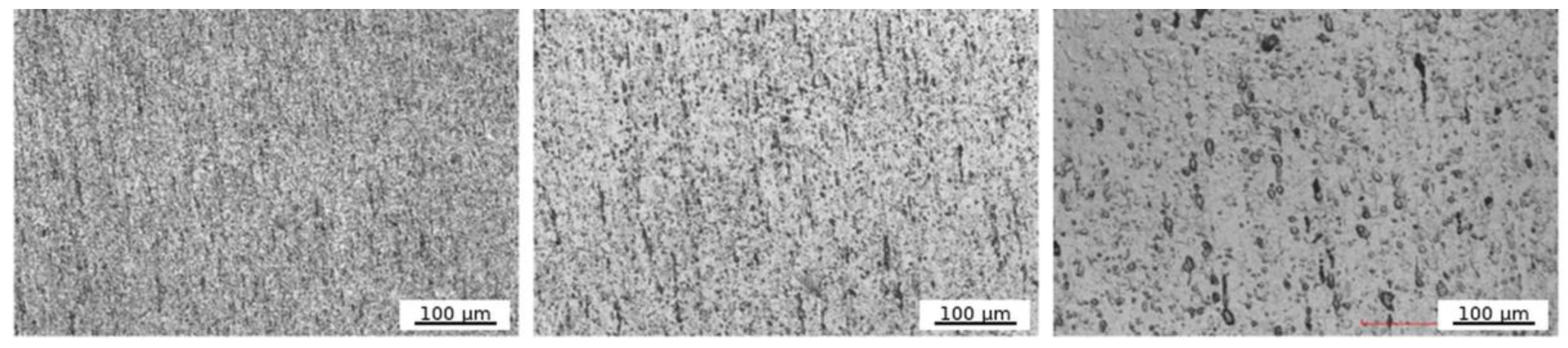
Figure 18.
Optical microstructure at the gauge edge of specimen T1 (450 °C, 10 rev s⁻¹). Grain elongation is less pronounced than at the center, reflecting the radial strain gradient in torsion. Scale bars shown in all panels.
Figure 18.
Optical microstructure at the gauge edge of specimen T1 (450 °C, 10 rev s⁻¹). Grain elongation is less pronounced than at the center, reflecting the radial strain gradient in torsion. Scale bars shown in all panels.
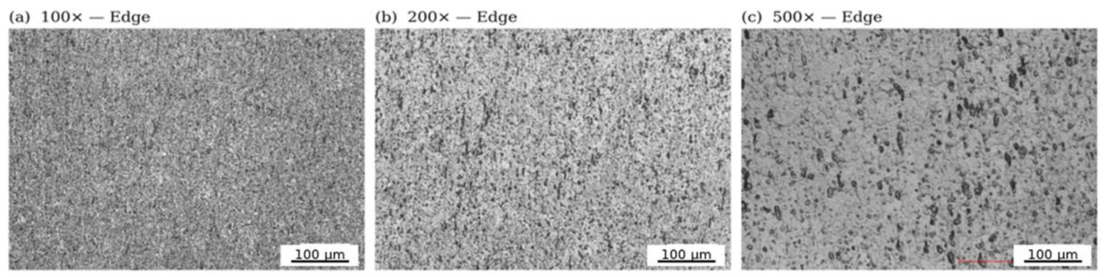

Table 1.
Nominal chemical composition of the AA6061-T6 extruded bar (wt.%, ASTM B221) and the specific batch composition used in this study. Balance Al.
Table 1.
Nominal chemical composition of the AA6061-T6 extruded bar (wt.%, ASTM B221) and the specific batch composition used in this study. Balance Al.
| Element | ASTM B221 range (wt.%) | Present batch (wt.%) |
|---|---|---|
| Si | 0.40–0.80 | 0.60 |
| Mg | 0.80–1.20 | 1.00 |
| Cu | 0.15–0.40 | 0.28 |
| Cr | 0.04–0.35 | 0.20 |
| Fe | ≤0.70 | 0.35 |
| Mn | ≤0.15 | 0.05 |
| Ti | ≤0.15 | 0.02 |
| Al | Balance | Balance |
Table 2.
Test conditions and key flow curve parameters. *T6 repeats T1 for reproducibility assessment. T/Tm computed using Tm = 582 °C.
Table 2.
Test conditions and key flow curve parameters. *T6 repeats T1 for reproducibility assessment. T/Tm computed using Tm = 582 °C.
| Spec. | T (°C) | T/Tm | ω (rev s⁻¹) | ε̇ (s⁻¹) | σp (MPa) | εp | εmax |
|---|---|---|---|---|---|---|---|
| T1 | 450 | 0.85 | 10 | 9.07 | 75.3 | 0.44 | 3.69 |
| T2 | 400 | 0.79 | 10 | 9.07 | 85.5 | 0.23 | 2.80 |
| T3 | 350 | 0.73 | 10 | 9.07 | 109.5 | 0.19 | 1.89 |
| T4 | 350 | 0.73 | 1 | 0.91 | 72.1 | 0.26 | 2.72 |
| T5 | 250 | 0.61 | 1 | 0.91 | 219.9 | 0.19 | 0.53 |
| T6* | 450 | 0.85 | 10 | 9.07 | 59.2 | 0.20 | 1.79 |
| T7 | 300 | 0.67 | 1 | 0.91 | 155.5 | 0.17 | 0.98 |
| T8 | 400 | 0.79 | 1 | 0.91 | 68.0 | 0.28 | 2.70 |
| T9 | 450 | 0.85 | 1 | 0.91 | 44.8 | 0.02 | 5.99 |
| T10 | 350 | 0.73 | 3 | 2.72 | 101.9 | 0.26 | 1.71 |
| T11 | 400 | 0.79 | 3 | 2.72 | 72.2 | 0.24 | 2.88 |
| T12 | 450 | 0.85 | 3 | 2.72 | 51.5 | 0.19 | 6.36 |
Table 3.
Visual inspection of selected specimens after hot torsion testing.
| Spec. | Condition | εmax | Macroscopic observation |
|---|---|---|---|
| T1 | 450 °C, 9.07 s⁻¹ | 3.69 | Partial fracture near one gauge end; large axial crack |
| T2 | 400 °C, 9.07 s⁻¹ | 2.80 | Near-complete separation at mid-gauge; axial misalignment |
| T3 | 350 °C, 9.07 s⁻¹ | 1.89 | Partial fracture on one side of mid-gauge |
| T9 | 450 °C, 0.91 s⁻¹ | 5.99 | No fracture; material accumulation near left gauge shoulder |
| T12 | 450 °C, 2.72 s⁻¹ | 6.36 | Circumferential crack across approximately ¾ of gauge diameter |
Table 4.
Garofalo–Arrhenius parameters for AA6061-T6 (T ≥ 300 °C, α = 0.045 MPa⁻¹) obtained by one-step nonlinear regression.
Table 4.
Garofalo–Arrhenius parameters for AA6061-T6 (T ≥ 300 °C, α = 0.045 MPa⁻¹) obtained by one-step nonlinear regression.
| Parameter | Symbol | Value | Units |
|---|---|---|---|
| Apparent activation energy | Q | 151.1 | kJ mol⁻¹ |
| Stress multiplier | α | 0.045 | MPa⁻¹ |
| Stress exponent | n | 1.371 | – |
| Pre-exponential factor | A | 3.51 × 10¹⁰ | s⁻¹ |
| Coefficient of determination | R² | 0.821 | – |
Table 5.
Upper-bound adiabatic temperature rise ΔTad at peak stress (Equation (6)). The Gleeble controller compensates a fraction of this heat; the true ΔTad is therefore lower than the tabulated values.
Table 5.
Upper-bound adiabatic temperature rise ΔTad at peak stress (Equation (6)). The Gleeble controller compensates a fraction of this heat; the true ΔTad is therefore lower than the tabulated values.
| Spec. | Tnom (°C) | ε̇ (s⁻¹) | σp (MPa) | εp | ΔTad (°C) | Teff (°C) |
|---|---|---|---|---|---|---|
| T1 | 450 | 9.07 | 75.3 | 0.44 | 12.3 | 462 |
| T2 | 400 | 9.07 | 85.5 | 0.23 | 7.3 | 407 |
| T3 | 350 | 9.07 | 109.5 | 0.19 | 7.7 | 358 |
| T4 | 350 | 0.91 | 72.1 | 0.26 | 7.0 | 357 |
| T7 | 300 | 0.91 | 155.5 | 0.17 | 9.8 | 310 |
| T8 | 400 | 0.91 | 68.0 | 0.28 | 7.1 | 407 |
| T9 | 450 | 0.91 | 44.8 | 0.02 | 0.3 | 450 |
| T10 | 350 | 2.72 | 101.9 | 0.26 | 9.9 | 360 |
| T11 | 400 | 2.72 | 72.2 | 0.24 | 6.4 | 406 |
| T12 | 450 | 2.72 | 51.5 | 0.19 | 3.6 | 454 |
Table 6.
Strain-compensated Arrhenius parameters at representative equivalent strain levels. N = number of conditions used at each level. α = 0.045 MPa⁻¹ held constant. Flow stresses estimated from Equation (7). ᵃ Rows at ε = 0.1–0.6 carry R² of 0.361–0.397, below the reliability threshold for independent use in FE simulation; these parameter values should not be applied outside the validated range (ε ≥ 0.8) without direct confirmation against measured flow curves.
Table 6.
Strain-compensated Arrhenius parameters at representative equivalent strain levels. N = number of conditions used at each level. α = 0.045 MPa⁻¹ held constant. Flow stresses estimated from Equation (7). ᵃ Rows at ε = 0.1–0.6 carry R² of 0.361–0.397, below the reliability threshold for independent use in FE simulation; these parameter values should not be applied outside the validated range (ε ≥ 0.8) without direct confirmation against measured flow curves.
| ε | N | n | Q (kJ mol⁻¹) | ln(A) | R² |
|---|---|---|---|---|---|
| 0.1a | 10 | 0.889 | 90.3 | 15.28 | 0.397 |
| 0.2a | 10 | 1.235 | 115.6 | 18.73 | 0.670 |
| 0.3a | 10 | 0.969 | 70.5 | 11.70 | 0.361 |
| 0.4a | 10 | 0.843 | 54.9 | 9.40 | 0.361 |
| 0.6a | 10 | 1.132 | 72.8 | 12.39 | 0.386 |
| 0.8 | 10 | 1.292 | 84.2 | 14.28 | 0.388 |
| 1.0 | 9 | 2.348 | 91.9 | 14.41 | 0.833 |
| 1.2 | 9 | 2.374 | 93.5 | 14.68 | 0.834 |
| 1.5 | 9 | 2.382 | 94.0 | 14.76 | 0.834 |
| 2.0 | 7 | 2.548 | 89.3 | 13.79 | 0.852 |
Table 7.
Comparison of Garofalo–Arrhenius parameters for AA6061 with prior literature. ᵃn = 1.371 from one-step torsion regression; lower than compression values due to the Nadai torque-integration geometry (see Section 8.1).
Table 7.
Comparison of Garofalo–Arrhenius parameters for AA6061 with prior literature. ᵃn = 1.371 from one-step torsion regression; lower than compression values due to the Nadai torque-integration geometry (see Section 8.1).
| Study | Test method | T range (°C) | ε̇ range (s⁻¹) | Q (kJ mol⁻¹) | n | α (MPa⁻¹) | AARE (%) |
|---|---|---|---|---|---|---|---|
| Rokni et al. [7] | Compression | 300–550 | 0.001–1 | 142.8 | 4.36 | 0.045 | 7.4 |
| Citrea et al. [9] | Compression | 300–550 | 0.01–10 | 156.8 | 4.12 | 0.045 | 5.8 |
| Qin et al. [10] | Compression | 350–500 | 0.001–1 | 148.3 | 3.89 | 0.040 | 6.2 |
| McQueen et al. [11] | Torsion | 300–550 | 0.1–10 | ~150 | ~4 | 0.04–0.05 | N/A |
| Present work | Torsion | 250–450 | 0.91–9.07 | 151.1 | 1.371ᵃ | 0.045 | 15.5 |
Disclaimer/Publisher’s Note: The statements, opinions and data contained in all publications are solely those of the individual author(s) and contributor(s) and not of MDPI and/or the editor(s). MDPI and/or the editor(s) disclaim responsibility for any injury to people or property resulting from any ideas, methods, instructions or products referred to in the content. |
© 2026 by the authors. Licensee MDPI, Basel, Switzerland. This article is an open access article distributed under the terms and conditions of the Creative Commons Attribution (CC BY) license (http://creativecommons.org/licenses/by/4.0/).
Copyright: This open access article is published under a Creative Commons CC BY 4.0 license, which permit the free download, distribution, and reuse, provided that the author and preprint are cited in any reuse.


