

Submitted:
02 July 2026
Posted:
03 July 2026
You are already at the latest version
Abstract
Monocular 3D lane detection is challenged by the loss of directional detail in distant markings during feature downsampling and by geometric ambiguity between lateral curvature and road elevation under single-view projection. R-A3D addresses both issues through frequency-aware Riemannian anchor learning in an anchor-regression pipeline. A Haar-based feature pyramid retains four frequency subbands before learned channel projection, strengthening thin and low-contrast lane responses. Each evolving 3D anchor is summarized in the lateral–elevation plane by Gaussian mean and covariance statistics, embedded in a symmetric positive-definite matrix, and mapped to a tangent-space feature with the Log-Euclidean metric. This Riemannian anchor feature is fused residually with anchor-aligned visual evidence and recomputed after each cascade stage. On OpenLane, the ResNet-50 model achieves 64.9% F1, 94.1% category accuracy, and far-range lateral and vertical errors of 0.215 m and 0.081 m at 23.5 frames/s; the ResNet-18 model reaches 63.0% F1 at 53.2 frames/s. On ApolloSim Visual Variations, R-A3D achieves 96.1% F1 and reduces the two far-range errors by 31.0% and 30.3% relative to GLane3D. These results demonstrate complementary benefits from frequency-preserving visual evidence and proposal-dependent Riemannian geometry.
Keywords:
monocular 3D lane detection
; frequency-aware learning
; Riemannian anchor learning
; discrete wavelet transform
; symmetric positive-definite matrix
; anchor-based detection
1. Introduction
Monocular 3D lane detection estimates lane instances as ordered point sets in a road-centered coordinate system from a single front-view image. The resulting lateral positions, longitudinal extents, and elevation profiles support lane keeping, trajectory planning, lane-level localization, and vector-map construction [1,2,3]. Accurate lane geometry also provides an important spatial basis for vehicle–lane interaction modeling and driving-risk assessment [4]. Compared with 2D lane detection, the task must recover metric 3D structure without direct depth sensing. The inverse projection is therefore ill-conditioned: perspective compression reduces distant markings to only a few pixels, while different combinations of road slope, lane curvature, and camera pose can produce similar image projections.
Existing monocular methods mainly follow depth-guided, bird’s-eye-view (BEV), curve-based, query-based, or anchor-based paradigms. Depth-guided methods lift image evidence through estimated depth [5,6]; BEV methods use inverse perspective mapping or learned view transformation [7,8,9]; structured methods describe lanes with splines, continuous curves, sparse points, or keypoint graphs [10,11,12,13]; and anchor-based methods directly regress 3D offsets from predefined lane hypotheses [14,15,16]. Recent work has further emphasized complete sparse-lane representation [13], road-height modeling [17,18], and temporal lane priors [19]. These advances reveal that representation completeness, road-surface geometry, temporal consistency, and image-feature quality are distinct but complementary dimensions of the problem.
R-A3D introduces a unified frequency-aware Riemannian anchor learning framework. Its central premise is that reliable anchor refinement requires both discriminative image evidence and a structure-aware representation of the current anchor state. Standard strided convolution and pooling can attenuate the high-frequency responses of distant, worn, shadowed, or weakly illuminated lane markings, while conventional Euclidean point sequences do not explicitly summarize the second-order relation between lateral variation and elevation change. R-A3D therefore couples fixed frequency decomposition with proposal-dependent SPD geometry: frequency-preserving features strengthen the visual observations used to update each anchor, and a Log-Euclidean descriptor summarizes the evolving lateral–elevation statistics during cascade refinement [20,21,22].
Riemannian geometry has recently been introduced into monocular 3D lane detection at different representation levels. For example, ReManNet studies lane–road relations under a road-manifold assumption and introduces a geometry-consistent overlap objective [23]. R-A3D addresses a different representation problem within a conventional anchor-regression pipeline. It does not learn a road-surface manifold or modify the matching objective; instead, it learns each predefined anchor through frequency-aware visual encoding, proposal-level SPD representation, and iterative coordinate refinement. This distinction places R-A3D at the anchor-learning level rather than at the road-manifold or loss-design level. The main contributions are summarized as follows:
- We propose a frequency-aware Riemannian anchor learning framework that couples frequency-preserving image evidence with the evolving second-order geometry of predefined 3D lane anchors in a cascaded regression pipeline.
- We develop a lightweight realization consisting of a four-subband Haar feature pyramid, an augmented Gaussian SPD representation, residual frequency–geometry interaction, and dynamic Log-Euclidean descriptor recomputation. The design preserves image-conditioned evidence while keeping the geometric representation synchronized with the current anchor state.
- Extensive experiments on OpenLane and ApolloSim evaluate detection accuracy, metric localization, scenario robustness, representation choices, repeatability, perturbation robustness, and same-hardware efficiency.
2. Related Work
2.1. Monocular 3D Lane Detection
3D-LaneNet and GenLaneNet construct BEV representations using inverse perspective mapping or geometric transformation [7,8]. PersFormer learns perspective-to-BEV associations with a transformer [9], while GP and CLGo introduce geometry and camera-pose constraints [24,25]. HeightLane predicts a multi-slope road height map to improve the spatial alignment of BEV features [17], and SC-Lane further adds slope-aware fusion and temporal height consistency [18]. These approaches exploit global road context but require an explicit or learned view transformation and may inherit errors from intermediate road-surface estimation.
Anchor3DLane and Anchor3DLane++ regress structured 3D lane hypotheses directly from front-view features [14,15]. At the image-plane representation level, angle-aware rectangle anchors have shown that fixed-width and fixed-direction anchor designs can introduce systematic geometric misalignment in lane detection [26]. Although that work focuses on 2D lane representations, it further motivates geometry-aware anchor design for structured lane estimation. LATR uses transformer-based lane representations [27]; LaneCPP introduces continuous physical curve priors [10]; PVALane aligns prior-guided features across views [16]; and GLane3D models lanes as graphs of 3D keypoints [12]. Chang et al. analyze endpoint truncation in sparse lane representations and introduce an endpoint patching strategy with PointLane attention [13]. SparseLaneSTP combines a continuous sparse representation with lane-specific spatial and temporal priors [19]. R-A3D remains single-frame and anchor-based, but treats visual frequency preservation and proposal-level Riemannian geometry as coupled parts of iterative anchor learning rather than as independent preprocessing and auxiliary encoding modules.
2.2. Frequency-Aware Neural Processing
Standard downsampling enlarges the receptive field but can remove narrow structures and introduce aliasing. Anti-aliased downsampling reduces shift sensitivity by low-pass filtering before decimation [28]. The discrete wavelet transform (DWT) performs a fixed multiresolution decomposition into approximation and directional detail subbands [29]. Wavelet pooling has been used to preserve information in convolutional networks [30], while wavelet-like transforms have been learned for compression and restoration [31,32]. Frequency-aware feature fusion has also improved dense prediction [33]. In 3D lane detection, Freq-3DLane uses frequency-aware front-view–BEV feature fusion [34]. R-A3D instead inserts a fixed Haar decomposition into the feature-pyramid downsampling path so that frequency-aware visual evidence directly conditions the Riemannian anchor learning loop, without requiring a BEV frequency-fusion branch.
2.3. SPD Geometry and Gaussian Descriptors
The SPD cone is a Riemannian manifold rather than a closed Euclidean vector space. Covariance descriptors can therefore be distorted by unconstrained Euclidean arithmetic. Log-Euclidean geometry defines a vector-space structure through the matrix logarithm [20]; Riemannian Gaussian models and geometry-aware neural networks further demonstrate the utility of SPD statistics in vision [21,35,36]. Within R-A3D, an augmented Gaussian embedding combines the mean and covariance of the current anchor coordinates and maps them to a tangent-space feature that represents the Riemannian state of the proposal. This anchor-level representation differs from road-manifold modeling approaches such as ReManNet [23]: the road surface is not estimated as a manifold, and the SPD object is constructed only from the evolving anchor coordinates. The descriptor represents structural dispersion and correlation; it is not interpreted as a calibrated posterior uncertainty estimate.
2.4. Positioning Relative to Recent Methods
Table 1 summarizes the architectural differences between R-A3D and representative recent detectors. The comparison is architectural rather than numerical because the methods use different training settings and, in some cases, additional temporal or height-map supervision. R-A3D occupies a BEV-free, single-frame design point and treats visual frequency preservation and proposal-level Riemannian geometry as coupled parts of anchor learning.
3. Materials and Methods
3.1. Problem Formulation and Coordinate System
Let the road-centered coordinate system use x for the lateral direction, y for the forward direction, and z for elevation. A lane instance j is represented by an ordered point set , together with a category label and point-wise visibility. Given camera intrinsics and the road-to-camera extrinsics , a 3D point projects to the image as
where is the projective depth. In the anchor representation, the longitudinal samples are predefined and the detector regresses lateral and vertical offsets. This formulation keeps the output compact, but the missing depth observation means that slope, lateral curvature, and camera pose remain coupled in the image domain.
3.2. Frequency-Aware Riemannian Anchor Learning Overview
Given a monocular image , R-A3D predicts category labels, visibility states, and ordered 3D points. Figure 1 shows the overall signal flow of frequency-aware Riemannian anchor learning. The visual pathway extracts frequency-aware evidence with a wavelet-enhanced feature pyramid network (W-FPN), while the geometric pathway represents each current anchor with an augmented Gaussian SPD descriptor. After Log-Euclidean mapping, the Riemannian anchor feature interacts residually with the anchor-aligned visual feature. Classification, visibility, and coordinate-regression heads then update the proposal, and the refined coordinates are used to reconstruct the SPD descriptor for the next cascade stage. The resulting loop alternates between visual sampling, Riemannian state encoding, frequency–geometry interaction, and coordinate refinement, so both information sources remain aligned with the evolving anchor. In this work, “anchor learning” denotes the joint feature encoding, geometric representation, and iterative coordinate refinement of predefined 3D anchors; it does not imply that the initial anchor set or its sampling positions are generated by a separate learnable anchor-generation network.
3.3. Wavelet-Enhanced Feature Pyramid
Let denote an intermediate feature map. A separable two-dimensional Haar transform applies low-pass and high-pass filters along the horizontal and vertical axes, followed by a factor-two decimation. The resulting feature tensor contains four subbands,
where is the low-frequency approximation and , , and encode directional details. The subbands are concatenated and projected by a convolution,
The Haar decomposition itself is invertible; however, the subsequent learned channel projection may be compressive. Accordingly, the design is described as information-preserving before projection rather than as an end-to-end lossless transform. The operation is inserted into the FPN downsampling path. For anchor j, the valid 3D points are projected into the image and converted to feature-map coordinates using the FPN stride. The minimum axis-aligned rectangle enclosing the valid projected points defines the sampling region; the region is clipped to the feature-map boundary, and anchors without valid projected support are masked. ROI Align [37] applies bilinear interpolation to obtain a fixed feature, which is globally averaged to produce the anchor-aligned visual feature .
Figure 2 shows the responses of the four subbands on a road image. The component retains the coarse road layout, whereas the directional detail components preserve lane boundaries, poles, and other high-frequency structures. R-A3D does not independently threshold these subbands; instead, their concatenated responses are learned by the subsequent projection. The resulting frequency-aware feature supplies the visual evidence used throughout the Riemannian anchor learning loop.
3.4. Riemannian Anchor State Encoding
The Riemannian state of an evolving anchor is constructed from its N ordered points . Because the longitudinal positions are predefined, the geometry descriptor is formed in the lateral–elevation plane with . The mean and regularized covariance are
where ensures numerical positive definiteness. The mean and covariance are embedded in an augmented Gaussian SPD matrix,
Using the eigendecomposition , the Log-Euclidean representation is
The upper-triangular entries of are vectorized and projected to dimensions by a multilayer perceptron, yielding . The diagonal terms encode lateral and elevation dispersion, whereas the off-diagonal term captures their global correlation over the sampled anchor. Because the statistic is computed over the complete anchor, it is invariant to permutations of the sampled points and does not localize where a curvature or elevation change occurs. The ordered coordinates remain available to the regression head through the anchor representation, while the SPD feature serves only as a compact complementary summary.
Figure 3 presents the construction of the descriptor. For a nearly straight and level anchor, the covariance ellipse is narrow; stronger curvature or elevation change increases its extent and rotates its principal axes. The augmented matrix combines the location of the anchor with this second-order structure. Because a symmetric matrix has six unique entries, the Log-Euclidean representation remains compact before the learned projection. A small diagonal regularizer prevents degenerate covariance when anchors are nearly straight. Importantly, the descriptor is deterministic and proposal-dependent: it captures geometric variability but does not claim probabilistic calibration.
3.5. Residual Frequency–Geometry Interaction
Each proposal provides one frequency-aware visual feature and one compact Riemannian anchor feature. Because the geometric pathway yields a single descriptor rather than a token sequence, R-A3D uses an explicit residual interaction instead of token-wise attention over a singleton key. The Riemannian anchor feature is first projected to the visual dimension,
and fused with the anchor-aligned visual feature,
This operation preserves the frequency-aware, image-conditioned anchor feature while introducing a proposal-dependent Riemannian residual. It is lightweight, avoids a quadratic token interaction, and remains well-defined for a single geometry descriptor. The fused representation is the learned anchor feature passed to the prediction heads.
3.6. Cascade Anchor Learning and Training Objective
At refinement stage t, the network predicts category scores, point visibility, and lateral and vertical offsets . The anchor update is
The mean, covariance, and Log-Euclidean descriptor are recomputed from . This dynamic re-encoding closes the Riemannian anchor learning loop by coupling the geometric representation to the current proposal state rather than to the initial anchor.
The total loss combines classification, coordinate regression, and visibility supervision,
Focal loss is used for sparse anchor classification [38]. For positive anchors, the regression loss is
where is the ground-truth visibility mask and is the Smooth L1 function. Binary cross-entropy supervises point visibility.
3.7. Computational Characteristics
Table 2 separates fixed analysis operations from learned projections. For an input feature map , the separable Haar analysis is linear in the number of input elements, whereas the following projection at spatial resolution has complexity . For each anchor, mean and covariance estimation are linear in the number of sampled points, and the matrix logarithm acts on a fixed SPD matrix. These expressions describe asymptotic operation counts; they do not replace hardware-level profiling because memory movement, kernel fusion, and eigendecomposition implementations can dominate practical latency.
4. Experimental Results
4.1. Datasets and Evaluation Protocol
R-A3D is evaluated on OpenLane and ApolloSim. OpenLane [9] contains approximately 200,000 real-world frames from 1000 sequences with camera intrinsics, extrinsics, and dense 3D lane annotations. It includes slopes, curves, intersections, merge/split regions, nighttime, and adverse-weather scenes. ApolloSim [8] contains 10,500 synthetic images with camera parameters and three official subsets: Balanced Scenes, Rare Subset, and Visual Variations. The Rare Subset represents long-tail road structures, whereas Visual Variations emphasize changes in illumination, weather, and appearance.
Following Anchor3DLane [14], lanes are sampled over m. A prediction is considered a true positive when at least 75% of its sampled points are within 1.5 m of the matched ground-truth lane. The evaluation reports F1 score, category accuracy, and lateral and vertical errors in the near (0–40 m) and far (40–100 m) ranges, denoted by , , , and .
4.2. Implementation and Reproducibility Details
The models use ImageNet-pretrained ResNet-18 or ResNet-50 backbones [39]. Images are resized to . The configuration uses 1000 initial anchor hypotheses, each sampled at longitudinal positions over m. The FPN output stride is 8, the geometry feature dimension is , and the cascade contains three refinement stages. For ROI Align, valid projected anchor points define a clipped rectangular region on the stride-8 FPN feature map; bilinear sampling produces a feature, followed by global average pooling before visual–geometric interaction. The six unique entries of the Log-Euclidean matrix are processed by a two-layer MLP with dimensions , GELU activations, and layer normalization. The covariance regularizer is .
AdamW is used with , , an initial learning rate of , weight decay of , and batch size 4. A 1000-iteration linear warm-up is followed by cosine decay. OpenLane and ApolloSim are trained for 60,000 and 50,000 iterations, respectively. Focal loss uses and , and the loss weights are , , and . Training augmentations include random brightness/contrast adjustment within , Gaussian blur with probability 0.1, and horizontal flipping with consistent updates to image coordinates, lane categories, and camera geometry. All repeatability experiments are conducted with three random seeds (0, 1, and 2), and the mean and standard deviation are reported. Training and runtime evaluation are performed on one NVIDIA GeForce RTX 4090 GPU with an AMD EPYC 9654 CPU under Python 3.10, PyTorch 2.4, CUDA 12.1, and cuDNN 9.1.
Anchor initialization, positive assignment, coordinate normalization, and the classification, regression, and visibility definitions follow our reimplementation of Anchor3DLane [14]. The reimplemented ResNet-50 baseline obtains 57.9% F1 on OpenLane, close to the 57.5% reported by the original publication. R-A3D retains the same anchor set, sampled longitudinal positions, assignment rule, output heads, and training objective; only the standard feature pyramid, proposal representation, and visual–geometric interaction are modified. This controlled setting attributes the measured differences to the proposed components rather than to changes in the evaluation, matching, or loss protocol.

Table 3.
Training and model configuration.
| Configuration | OpenLane | ApolloSim |
|---|---|---|
| Input resolution | ||
| Backbone | ResNet-18/50 | ResNet-18/50 |
| Initial anchors / sampled points | 1000 / 20 | 1000 / 20 |
| FPN output stride | 8 | 8 |
| ROI Align output | ||
| Geometry MLP | ||
| Covariance regularizer | ||
| Cascade stages | 3 | 3 |
| Optimizer / batch size | AdamW / 4 | AdamW / 4 |
| Initial learning rate | ||
| Loss weights | ||
| Training iterations | 60,000 | 50,000 |
| Software | Python 3.10; PyTorch 2.4; CUDA 12.1; cuDNN 9.1 | |
| Hardware | One NVIDIA GeForce RTX 4090 GPU; AMD EPYC 9654 CPU | |
The experimental evaluation examines R-A3D from six complementary perspectives: overall detection accuracy and metric localization, performance under visually degraded and elevation-varying conditions, the contribution of key architectural choices, stability across random seeds, robustness to image degradation and camera-calibration perturbations, and the accuracy–efficiency trade-off under identical hardware conditions. Unless otherwise stated, the controlled ablations and efficiency profile use the reimplemented Anchor3DLane baseline described above, whereas the perturbation experiment reports the sensitivity of the complete R-A3D model. All models use single-frame monocular input without temporal cues, LiDAR supervision, or test-time map information. Throughput values reported in prior publications are included only for contextual reference, whereas Table 13 presents measurements obtained under the unified hardware and software protocol.
4.3. OpenLane Overall Accuracy
Table 4 reports the overall OpenLane results. R-A3D with ResNet-50 achieves 64.9% F1 and 94.1% category accuracy. Relative to Anchor3DLane++ with the same backbone, it improves F1 by 2.5 percentage points and reduces the far-range lateral and vertical errors from 0.237 m and 0.100 m to 0.215 m and 0.081 m, corresponding to relative reductions of 9.3% and 19.0%. The larger reduction in is consistent with the explicit lateral–elevation covariance descriptor. The ResNet-18 configuration retains 63.0% F1, providing a lightweight alternative. Published FPS values in Table 4 are included only for context because they were obtained under heterogeneous hardware and software settings; the controlled same-hardware analysis is reported in Table 13.
4.4. Scenario-Wise Robustness on OpenLane
Scenario-wise results are shown in Table 5. R-A3D obtains the best F1 scores for up/down slopes, extreme weather, nighttime, and intersections. Relative to Anchor3DLane++, the gains in these four subsets are 6.7, 4.1, 6.4, and 6.2 percentage points, respectively. The slope result supports the role of lateral–elevation statistics, while the weather and night results are consistent with directional detail preservation. R-A3D is not the best on curves or merge/split cases. These failure modes require long-range curve reasoning or explicit inter-lane connectivity, which are only indirectly represented by a single-anchor covariance descriptor.
4.5. ApolloSim Results
Table 6 reports results on the three official ApolloSim subsets. On balanced scenes, R-A3D is competitive and achieves the lowest far-range lateral error. On the Rare subset, it obtains the lowest far-range lateral error despite an F1 score below GLane3D. On Visual Variations, R-A3D reaches 96.1% F1, 3.4 percentage points above GLane3D, while reducing and by 31.0% and 30.3% relative to GLane3D. The vertical error of 0.221 m is competitive but is slightly above the best reported value of 0.219 m from Anchor3DLane.
4.6. Component Ablation and Complementarity
Table 7 isolates the successive stages of the proposed anchor learning framework on OpenLane with ResNet-50, starting from the reimplemented Anchor3DLane baseline. Replacing its standard FPN with W-FPN increases F1 from 57.9% to 59.5% and reduces both far-range errors. Adding the Riemannian anchor state raises F1 to 61.5% and reduces to 0.110 m. Residual frequency–geometry interaction together with dynamic descriptor re-encoding yields 64.9% F1 and the lowest far-range errors. The progressive gains support the central design: reliable anchor learning benefits from frequency-aware visual evidence, proposal-level Riemannian geometry, and their synchronized interaction.
4.7. Controlled Downsampling Alternatives
Table 8 reports a controlled comparison between standard, anti-aliased, and wavelet-based downsampling. BlurPool improves over strided convolution, confirming that aliasing contributes to the loss of thin lane responses. Retaining only the Haar LL component offers a similar improvement but omits directional details. Four-subband Haar decomposition achieves the best F1 and localization errors while remaining faster than the longer Daubechies-2 filters. The comparison supports the use of all four Haar subbands rather than attributing the gain merely to a larger channel tensor.
4.8. Geometry-Representation Alternatives
Table 9 separates the contribution of the statistical representation from the contribution of the SPD geometry. A raw-coordinate MLP already improves over using no geometry, showing that proposal coordinates are informative. Adding covariance is more effective than using the mean alone. Cholesky parameterization provides a positive-definite representation, but the Log-Euclidean mapping gives the best result, particularly for far-range elevation. This pattern is consistent with a geometry-aware treatment of covariance rather than unconstrained Euclidean vectorization.
4.9. Frequency–Geometry Interaction and Dynamic Riemannian Re-encoding
Table 10 evaluates the interaction stage while holding the frequency-aware visual pathway and Riemannian state encoding fixed. Static concatenation is the weakest option. Gating and residual interaction preserve the original image-conditioned evidence more effectively, and recomputing the Riemannian descriptor after every cascade stage contributes a further 1.2 F1 points over static residual fusion. The result supports the closed-loop anchor learning design: the geometric state should follow the refined proposal instead of remaining tied to the initial anchor.
4.10. Repeatability Across Random Seeds
Table 11 reports random-seed stability. The standard deviations are small relative to the observed improvements, and the performance gaps between successive configurations are larger than the measured run-to-run variation. This analysis distinguishes the gains of the proposed components from normal optimization variability.
4.11. Robustness to Image and Calibration Perturbations
Table 12 reports a sensitivity analysis of the complete R-A3D model under controlled image degradation and camera-model errors. All perturbations are applied only at test time to the same evaluation images, using the clean-data checkpoint without retraining or test-time adaptation. Brightness reduction multiplies RGB intensities by 0.7 followed by clipping to the valid range. Gaussian blur uses , and JPEG compression performs one encode–decode cycle at quality 40. The synthetic-rain condition uses a fixed moderate preset and fixed random seed. Camera perturbations modify only the calibration supplied to the detector: pitch and roll offsets are applied to the road-to-camera rotation, and the focal-length perturbation scales and by 1.05 while leaving the principal point unchanged. The input image and ground-truth 3D lanes remain fixed, so these tests measure sensitivity to image degradation and calibration mismatch rather than adaptation. R-A3D retains 92.1–96.6% of its clean F1 under the evaluated appearance perturbations and 89.4–96.5% under the evaluated camera perturbations. The method remains calibration dependent and should not be interpreted as invariant to camera-model errors.
4.12. Controlled Same-Hardware Efficiency Profile
Table 13 reports a controlled efficiency profile using batch size 1 and FP32 inference. Each latency value is averaged over 1000 synchronized runs after 200 warm-up iterations. Relative to the reimplemented Anchor3DLane baseline, the complete R-A3D model adds 0.6 M parameters, 1.0 GFLOPs, and 0.23 GB peak memory, while reducing throughput from 25.5 to 23.5 frames/s. The ResNet-18 version remains a useful high-throughput operating point. Reporting the full measurement protocol prevents heterogeneous published FPS values from being interpreted as a controlled comparison.
4.13. Qualitative Analysis
Figure 4 compares R-A3D with Anchor3DLane and Anchor3DLane++ in daytime multi-lane, curved-road, occluded/complex-geometry, and nighttime scenes. Anchor3DLane exhibits visible far-range drift, while Anchor3DLane++ shows local fragmentation in weakly illuminated regions. R-A3D more consistently preserves lane continuity and the elevation trend in the 3D view. The figure is qualitative and does not establish metric superiority by itself, but the visual patterns agree with the lower far-range errors and the gains on nighttime, adverse-weather, and slope subsets.
5. Discussion
The experimental results indicate that frequency-aware visual evidence and proposal-level Riemannian geometry play complementary roles in anchor refinement. Frequency-preserving features improve the reliability of image observations for distant and low-contrast lane markings, whereas the SPD representation provides the refinement process with proposal-dependent second-order geometric context. The incremental ablation shows that the visual pathway, Riemannian state encoding, and residual interaction each contribute to the final performance. The controlled downsampling experiments further indicate that the visual improvement cannot be attributed only to anti-aliasing. In particular, the comparison between the LL-only and four-subband variants supports the benefit of retaining directional detail. Similarly, raw coordinates and Euclidean covariance already provide useful proposal information, while the Log-Euclidean SPD representation achieves the lowest far-range vertical error among the evaluated geometric encodings.
The interaction experiments clarify why R-A3D is formulated as an iterative anchor-learning framework rather than as static feature augmentation. A descriptor computed only from the initial proposal becomes increasingly inconsistent as cascade refinement changes the anchor coordinates. Residual interaction preserves the image-conditioned visual feature, while dynamic re-encoding updates the geometric state after each refinement stage. The resulting closed loop keeps the visual observation and the Riemannian descriptor aligned with the current anchor proposal. In addition, the improvements across the ablation configurations are substantially larger than the measured run-to-run variation over three random seeds, indicating that the gains are stable under different training initializations.
The robustness and efficiency experiments further characterize the practical behavior of the method. Under reduced illumination, blur, compression, and synthetic rain, R-A3D retains 92.1–96.6% of its clean-input F1, which is consistent with the preservation of directional frequency components. Under moderate pitch, roll, and focal-length perturbations, the retention ranges from 89.4% to 96.5%, with the largest decrease occurring at a pitch offset. These results indicate tolerance to moderate calibration mismatch, but the method remains dependent on accurate camera parameters. Under the unified hardware protocol, the complete R50 model adds 0.6 M parameters, 1.0 GFLOPs, 0.23 GB of peak memory, and 3.4 ms of latency relative to the reimplemented Anchor3DLane baseline, while improving both F1 score and far-range localization. The R18 configuration provides a higher-throughput operating point at 53.2 frames/s. Further deployment studies should evaluate mixed-precision inference, power consumption, thermal stability, and end-to-end latency including image preprocessing and lane postprocessing.
Several limitations remain. First, the global covariance descriptor is permutation invariant and therefore cannot identify where curvature or elevation changes occur along the longitudinal direction. Local SPD windows or an ordered geometric encoder may preserve this information more effectively. Second, R-A3D processes individual frames and does not explicitly model temporal consistency or inter-lane topology, which is consistent with its weaker performance on curved and merge/split scenes. Third, the SPD descriptor summarizes structural dispersion and correlation but should not be interpreted as a calibrated uncertainty estimate. Finally, evaluation is limited to OpenLane and ApolloSim, and the latter is synthetic; consequently, cross-dataset and cross-domain generalization remain to be investigated.
6. Conclusions
This work presented R-A3D, a frequency-aware Riemannian anchor learning framework for monocular 3D lane detection. Rather than treating frequency preservation and geometric encoding as isolated modules, R-A3D couples directional image evidence with the evolving second-order statistics of each predefined 3D anchor. A Haar-based feature pyramid preserves weak lane responses, an augmented Gaussian SPD representation provides a compact Log-Euclidean description of the current anchor state, and residual interaction with dynamic re-encoding maintains frequency–geometry consistency throughout cascade refinement. On OpenLane, R-A3D with ResNet-50 achieves 64.9% F1 and reduces far-range lateral and vertical errors to 0.215 m and 0.081 m; the ResNet-18 configuration provides a 53.2 frames/s alternative. On ApolloSim Visual Variations, the method obtains 96.1% F1 and substantially reduces far-range errors relative to GLane3D.
The controlled experiments further substantiate the frequency decomposition, Riemannian representation, interaction mechanism, dynamic anchor-state update, and same-hardware efficiency. Future work will investigate ordered local SPD descriptors, explicit lane topology, temporal fusion, calibrated uncertainty, and target-platform quantization.
Author Contributions
Conceptualization, C.H. and B.L.; methodology, C.H.; software, C.H.; validation, C.H.; formal analysis, C.H.; investigation, C.H.; resources, B.L.; data curation, C.H.; writing—original draft preparation, C.H.; writing—review and editing, C.H. and B.L.; visualization, C.H.; supervision, B.L.; project administration, B.L.; funding acquisition, B.L. All authors have read and agreed to the published version of the manuscript.
Funding
This research was funded by the Department of Science and Technology of Hubei Province, grant number 2023BAB146.
Institutional Review Board Statement
Not applicable.
Informed Consent Statement
Not applicable.
Data Availability Statement
The OpenLane dataset is publicly available at https://github.com/OpenDriveLab/OpenLane. The ApolloSim dataset is publicly available at https://github.com/yuliangguo/3D_Lane_Synthetic_Dataset. No new dataset was created. The source code, configuration files, and evaluation scripts will be made publicly available upon publication.
Acknowledgments
The authors thank the developers and maintainers of the OpenLane and ApolloSim benchmarks.
Conflicts of Interest
The authors declare no conflicts of interest. The funder had no role in the design of the study; in the collection, analyses, or interpretation of data; in the writing of the manuscript; or in the decision to publish the results.
Abbreviations
The following abbreviations are used in this manuscript:
| BEV | Bird’s-eye view |
| DWT | Discrete wavelet transform |
| FPN | Feature pyramid network |
| ROI | Region of interest |
| SPD | Symmetric positive-definite |
| W-FPN | Wavelet-enhanced feature pyramid network |
References
- Chen, Z.; Huang, X. End-to-End Learning for Lane Keeping of Self-Driving Cars. In Proceedings of the IEEE Intelligent Vehicles Symposium (IV), 2017; pp. 1856–1860. [Google Scholar] [CrossRef]
- Zhu, S.; Aksun-Guvenc, B. Trajectory Planning of Autonomous Vehicles Based on Parameterized Control Optimization in Dynamic On-Road Environments. J. Intell. Robot. Syst. 2020, 100, 1055–1067. [Google Scholar] [CrossRef]
- Ma, F.; Qi, W.; Zhao, G.; Zheng, L.; Wang, S.; Liu, Y.; Liu, M.; Ma, J. Monocular 3D Lane Detection for Autonomous Driving: Recent Achievements, Challenges, and Outlooks. IEEE Trans. Intell. Transp. Syst. 2025, 26, 7380–7400. [Google Scholar] [CrossRef]
- Ma, Z.; Zhang, H.; Hong, C.; Xu, S.; Zhang, D.; Zhou, J.; Chen, Z.; Li, B. Modeling of Driving Risk Fields Considering Vehicle–Lane Interactions and Its Application in Car-Following Model. Phys. A Stat. Mech. Its Appl. 2026, 681, 131086. [Google Scholar] [CrossRef]
- Yan, F.; Nie, M.; Cai, X.; Han, J.; Xu, H.; Yang, Z.; Ye, C.; Fu, Y.; Mi, M.B.; Zhang, L. ONCE-3DLanes: Building Monocular 3D Lane Detection. In Proceedings of the IEEE/CVF Conference on Computer Vision and Pattern Recognition (CVPR), 2022; pp. 17143–17152. [Google Scholar]
- Luo, Y.; Yan, X.; Zheng, C.; Zheng, C.; Mei, S.; Tang, K.; Cui, S.; Li, Z. M2-3DLaneNet: Exploring Multi-Modal 3D Lane Detection. arXiv 2022, arXiv:2209.05996. [Google Scholar]
- Garnett, N.; Cohen, R.; Pe’er, T.; Lahav, R.; Levi, D. 3D-LaneNet: End-to-End 3D Multiple Lane Detection. In Proceedings of the IEEE/CVF International Conference on Computer Vision (ICCV), 2019; pp. 2921–2930. [Google Scholar]
- Guo, Y.; Chen, G.; Zhao, P.; Zhang, W.; Miao, J.; Wang, J.; Choe, T.E. Gen-LaneNet: A Generalized and Scalable Approach for 3D Lane Detection. In Proceedings of the European Conference on Computer Vision (ECCV), 2020; pp. 666–681. [Google Scholar] [CrossRef]
- Chen, L.; Sima, C.; Li, Y.; Zheng, Z.; Xu, J.; Geng, X.; Li, H.; He, C.; Shi, J.; Qiao, Y. PersFormer: 3D Lane Detection via Perspective Transformer and the OpenLane Benchmark. In Proceedings of the European Conference on Computer Vision (ECCV), 2022; pp. 550–567. [Google Scholar] [CrossRef]
- Pittner, M.; Janai, J.; Condurache, A.P. LaneCPP: Continuous 3D Lane Detection Using Physical Priors. In Proceedings of the IEEE/CVF Conference on Computer Vision and Pattern Recognition (CVPR), 2024; pp. 10639–10648. [Google Scholar]
- Bai, Y.; Chen, Z.; Fu, Z.; Peng, L.; Liang, P.; Cheng, E. CurveFormer: 3D Lane Detection by Curve Propagation with Curve Queries and Attention. In Proceedings of the IEEE International Conference on Robotics and Automation (ICRA), 2023; pp. 7062–7068. [Google Scholar] [CrossRef]
- Öztürk, H.İ.; Kalfaoğlu, M.E.; Kilinc, O. GLane3D: Detecting Lanes with Graphs of 3D Keypoints. In Proceedings of the IEEE/CVF Conference on Computer Vision and Pattern Recognition (CVPR), 2025; pp. 27508–27518. [Google Scholar]
- Chang, Y.; Huang, J.; Wang, X.; Ye, Y.; Liang, Z.; Shan, Y.; Du, D.; Wang, X. Rethinking Lanes and Points in Complex Scenarios for Monocular 3D Lane Detection. Proc. IEEE/CVF Conf. Comput. Vis. Pattern Recognit. (CVPR) 2025, 6802–6811. [Google Scholar] [CrossRef]
- Huang, S.; Shen, Z.; Huang, Z.; Ding, Z.; Dai, J.; Han, J.; Wang, N.; Liu, S. Anchor3DLane: Learning to Regress 3D Anchors for Monocular 3D Lane Detection. In Proceedings of the IEEE/CVF Conference on Computer Vision and Pattern Recognition (CVPR), 2023; pp. 17451–17460. [Google Scholar]
- Huang, S.; Shen, Z.; Huang, Z.; Liao, Y.; Han, J.; Wang, N.; Liu, S. Anchor3DLane++: 3D Lane Detection via Sample-Adaptive Sparse 3D Anchor Regression. IEEE Trans. Pattern Anal. Mach. Intell. 2025, 47, 1660–1673. [Google Scholar] [CrossRef] [PubMed]
- Zheng, Z.; Zhang, X.; Mou, Y.; Gao, X.; Li, C.; Huang, G.; Pun, C.M.; Yuan, X. PVALane: Prior-Guided 3D Lane Detection with View-Agnostic Feature Alignment. Proc. AAAI Conf. Artif. Intell. 2024, 38, 7597–7604. [Google Scholar] [CrossRef]
- Park, C.; Seo, E.; Lim, J. HeightLane: BEV Heightmap Guided 3D Lane Detection. In Proceedings of the IEEE/CVF Winter Conference on Applications of Computer Vision (WACV), 2025; pp. 1692–1701. [Google Scholar]
- Park, C.; Seo, E.; Hwang, J.; Lim, J. SC-Lane: Slope-Aware and Consistent Road Height Estimation Framework for 3D Lane Detection. In Proceedings of the IEEE/CVF International Conference on Computer Vision (ICCV), 2025; pp. 28407–28416. [Google Scholar]
- Pittner, M.; Janai, J.; Faigle, M.; Condurache, A.P. SparseLaneSTP: Leveraging Spatio-Temporal Priors with Sparse Transformers for 3D Lane Detection. In Proceedings of the IEEE/CVF International Conference on Computer Vision (ICCV), 2025; pp. 29099–29109. [Google Scholar]
- Arsigny, V.; Fillard, P.; Pennec, X.; Ayache, N. Geometric Means in a Novel Vector Space Structure on Symmetric Positive-Definite Matrices. SIAM J. Matrix Anal. Appl. 2007, 29, 328–347. [Google Scholar] [CrossRef]
- Said, S.; Bombrun, L.; Berthoumieu, Y.; Manton, J.H. Riemannian Gaussian Distributions on the Space of Symmetric Positive-Definite Matrices. IEEE Trans. Inf. Theory 2017, 63, 2153–2170. [Google Scholar] [CrossRef]
- Li, P.; Wang, Q.; Zeng, H.; Zhang, L. Local Log-Euclidean Multivariate Gaussian Descriptor and Its Application to Image Classification. IEEE Trans. Pattern Anal. Mach. Intell. 2017, 39, 803–817. [Google Scholar] [CrossRef] [PubMed]
- Hong, C.; Li, B. ReManNet: A Riemannian Manifold Network for Monocular 3D Lane Detection. In Proceedings of the IEEE/CVF Conference on Computer Vision and Pattern Recognition (CVPR), 2026; pp. 33046–33056. [Google Scholar]
- Li, C.; Shi, J.; Wang, Y.; Cheng, G. Reconstruct from Top View: A 3D Lane Detection Approach Based on Geometry Structure Prior. In Proceedings of the IEEE/CVF Conference on Computer Vision and Pattern Recognition Workshops (CVPRW), 2022; pp. 4370–4379. [Google Scholar]
- Liu, R.; Chen, D.; Liu, T.; Xiong, Z.; Yuan, Z. Learning to Predict 3D Lane Shape and Camera Pose from a Single Image via Geometry Constraints. Proc. AAAI Conf. Artif. Intell. 2022, 36, 1765–1772. [Google Scholar] [CrossRef]
- Hong, C.; Wang, Z.; Ma, Z.; Zhi, M.; Li, B. Angle-Aware Rectangle Anchors for Lane Detection: Addressing Geometric Misalignments in Anchor-Based Representations. IEEE Transactions on Geoscience and Remote Sensing, 2026; Early Access. [Google Scholar] [CrossRef]
- Luo, Y.; Zheng, C.; Yan, X.; Tang, K.; Zheng, C.; Cui, S.; Li, Z. LATR: 3D Lane Detection from Monocular Images with Transformer. In Proceedings of the IEEE/CVF International Conference on Computer Vision (ICCV), 2023; pp. 7941–7952. [Google Scholar]
- Zhang, R. Making Convolutional Networks Shift-Invariant Again. In Proceedings of the International Conference on Machine Learning (ICML), 2019; pp. 7324–7334. [Google Scholar]
- Mallat, S. A Wavelet Tour of Signal Processing; Academic Press: San Diego, CA, USA, 1999. [Google Scholar]
- Williams, T.; Li, R. Wavelet Pooling for Convolutional Neural Networks. In Proceedings of the International Conference on Learning Representations (ICLR), 2018. [Google Scholar]
- Ma, H.; Liu, D.; Xiong, R.; Wu, F. iWave: CNN-Based Wavelet-Like Transform for Image Compression. IEEE Trans. Multimed. 2020, 22, 1667–1679. [Google Scholar]
- Pimpalkhute, V.A.; Page, R.; Kothari, A.; Bhurchandi, K.M.; Kamble, V.M. Digital Image Noise Estimation Using DWT Coefficients. IEEE Trans. Image Process. 2021, 30, 1962–1972. [Google Scholar] [CrossRef] [PubMed]
- Chen, L.; Fu, Y.; Gu, L.; Yan, C.; Harada, T.; Huang, G. Frequency-Aware Feature Fusion for Dense Image Prediction. IEEE Trans. Pattern Anal. Mach. Intell. 2024, 46, 10763–10780. [Google Scholar] [CrossRef] [PubMed]
- Song, Y.; Bi, J.; Sun, L.; Liu, Z.; Jiang, Y.; Wang, X. Freq-3DLane: 3D Lane Detection from Monocular Images via Frequency-Aware Feature Fusion. IEEE Trans. Intell. Transp. Syst. 2025, 26, 12974–12986. [Google Scholar]
- Lin, T.; Zha, H. Riemannian Manifold Learning. IEEE Trans. Pattern Anal. Mach. Intell. 2008, 30, 796–809. [Google Scholar] [CrossRef] [PubMed]
- Nguyen, X.S. GeomNet: A Neural Network Based on Riemannian Geometries of SPD Matrix Space and Cholesky Space for 3D Skeleton-Based Interaction Recognition. In Proceedings of the IEEE/CVF International Conference on Computer Vision (ICCV), 2021; pp. 13379–13389. [Google Scholar]
- He, K.; Gkioxari, G.; Dollár, P.; Girshick, R. Mask R-CNN. In Proceedings of the IEEE International Conference on Computer Vision (ICCV), 2017; pp. 2961–2969. [Google Scholar]
- Lin, T.Y.; Goyal, P.; Girshick, R.; He, K.; Dollár, P. Focal Loss for Dense Object Detection. IEEE Trans. Pattern Anal. Mach. Intell. 2020, 42, 318–327. [Google Scholar] [CrossRef] [PubMed]
- He, K.; Zhang, X.; Ren, S.; Sun, J. Deep Residual Learning for Image Recognition. In Proceedings of the IEEE Conference on Computer Vision and Pattern Recognition (CVPR), 2016; pp. 770–778. [Google Scholar]
Figure 1.
Overview of the proposed frequency-aware Riemannian anchor learning framework. DWT denotes discrete wavelet transform; W-FPN denotes wavelet-enhanced feature pyramid network; ROI denotes region of interest; SPD denotes symmetric positive-definite; and CLS and Reg denote classification and regression, respectively. The visual pathway preserves the four Haar subbands before learned channel projection. Each predefined 3D anchor is represented by a Log-Euclidean SPD descriptor that interacts residually with anchor-aligned visual evidence. Anchor coordinates and their Riemannian descriptors are updated together throughout cascade refinement.
Figure 1.
Overview of the proposed frequency-aware Riemannian anchor learning framework. DWT denotes discrete wavelet transform; W-FPN denotes wavelet-enhanced feature pyramid network; ROI denotes region of interest; SPD denotes symmetric positive-definite; and CLS and Reg denote classification and regression, respectively. The visual pathway preserves the four Haar subbands before learned channel projection. Each predefined 3D anchor is represented by a Log-Euclidean SPD descriptor that interacts residually with anchor-aligned visual evidence. Anchor coordinates and their Riemannian descriptors are updated together throughout cascade refinement.
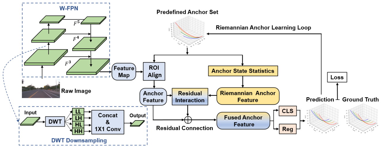
Figure 2.
Haar decomposition of a road image. The subband preserves coarse appearance, while , , and retain directional edge responses that are relevant to thin lane markings. The displayed detail magnitudes are normalized for visualization.
Figure 2.
Haar decomposition of a road image. The subband preserves coarse appearance, while , , and retain directional edge responses that are relevant to thin lane markings. The displayed detail magnitudes are normalized for visualization.

Figure 3.
Geometric interpretation of the Riemannian anchor descriptor. (a) Ordered anchor points are summarized in the lateral–elevation plane by a mean and covariance ellipse. (b) First- and second-order statistics are embedded in an augmented SPD matrix. (c) The matrix logarithm and half-vectorization produce a compact tangent-space feature. The schematic visualizes the descriptor construction and does not represent calibrated predictive uncertainty.
Figure 3.
Geometric interpretation of the Riemannian anchor descriptor. (a) Ordered anchor points are summarized in the lateral–elevation plane by a mean and covariance ellipse. (b) First- and second-order statistics are embedded in an augmented SPD matrix. (c) The matrix logarithm and half-vectorization produce a compact tangent-space feature. The schematic visualizes the descriptor construction and does not represent calibrated predictive uncertainty.
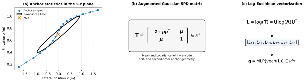
Figure 4.
Qualitative comparison on OpenLane. Columns show Anchor3DLane, Anchor3DLane++, and R-A3D; rows show representative daytime/multi-lane, curved-road, complex-geometry, and nighttime scenes. Red curves denote ground truth, and the remaining colors denote predicted lane categories.
Figure 4.
Qualitative comparison on OpenLane. Columns show Anchor3DLane, Anchor3DLane++, and R-A3D; rows show representative daytime/multi-lane, curved-road, complex-geometry, and nighttime scenes. Red curves denote ground truth, and the remaining colors denote predicted lane categories.
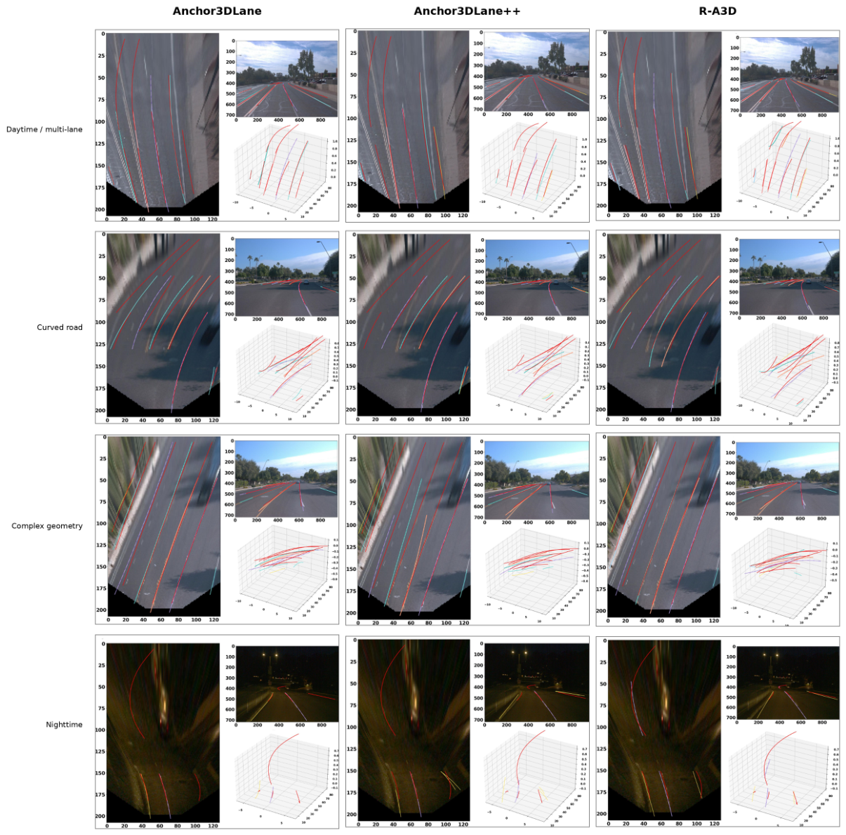
Table 1.
Architectural comparison with representative recent monocular 3D lane detectors. BEV denotes bird’s-eye view; Freq. denotes frequency-aware processing; and SPD denotes symmetric positive-definite.
Table 1.
Architectural comparison with representative recent monocular 3D lane detectors. BEV denotes bird’s-eye view; Freq. denotes frequency-aware processing; and SPD denotes symmetric positive-definite.
| Method | Representation | BEV-Free | Freq. | Temporal | Structural Mechanism |
|---|---|---|---|---|---|
| Anchor3DLane++ [15] | Sparse 3D anchors | Yes | No | No | Sample-adaptive sparse anchors |
| Freq-3DLane [34] | Front-view/BEV features | No | Yes | No | Cross-view frequency fusion |
| HeightLane [17] | BEV features + height map | No | No | No | Multi-slope height guidance |
| Chang et al. [13] | Patched sparse points | Yes | No | No | Endpoint completion + PointLane attention |
| GLane3D [12] | Graph of 3D keypoints | Yes | No | No | 3D keypoint graph connectivity |
| SparseLaneSTP [19] | Continuous sparse lanes | Yes | No | Yes | Lane-specific spatial–temporal prior |
| SC-Lane [18] | Height map + lane detector | No | No | Yes | Temporal slope-aware height estimation |
| R-A3D | Sparse 3D anchors + SPD descriptor | Yes | Yes | No | Frequency-aware Riemannian anchor refinement |
Table 2.
Analytical computational characteristics of the proposed components. H, W, and denote input feature-map dimensions; is the projected channel dimension; N is the number of points per anchor; and is the geometry-feature dimension.
Table 2.
Analytical computational characteristics of the proposed components. H, W, and denote input feature-map dimensions; is the projected channel dimension; N is the number of points per anchor; and is the geometry-feature dimension.
| Component | Operation | Analytical Cost |
|---|---|---|
| Fixed Haar analysis | Four separable low-/high-pass subbands with factor-two decimation | ; no trainable filter coefficients |
| Channel projection | Concatenation followed by a convolution at | |
| Anchor statistics | Mean and covariance in the lateral–elevation plane | per anchor |
| SPD logarithm | Eigendecomposition and logarithm of a matrix | Constant-size matrix operation per anchor |
| Geometry projection and fusion | MLP/linear projection, addition, and layer normalization | per anchor |
| Cascade recomputation | Coordinate update and repeated descriptor construction | Linear in anchors, points, and refinement stages |
Table 4.
Overall performance comparison on OpenLane. Best F1, category-accuracy, and localization results are highlighted in bold. Reported FPS values are provided for reference only because the original methods were evaluated under heterogeneous hardware and software settings.
Table 4.
Overall performance comparison on OpenLane. Best F1, category-accuracy, and localization results are highlighted in bold. Reported FPS values are provided for reference only because the original methods were evaluated under heterogeneous hardware and software settings.
| Method | F1 (%) |
Cat. Acc. (%) |
Speed (FPS) |
Localization Error (m) | |||
|---|---|---|---|---|---|---|---|
| 3D-LaneNet [7] | 44.1 | – | 67.5 | 0.479 | 0.572 | 0.367 | 0.443 |
| GenLaneNet [8] | 32.3 | – | 16.6 | 0.591 | 0.684 | 0.411 | 0.521 |
| PersFormer [9] | 50.5 | 92.3 | 18.1 | 0.485 | 0.553 | 0.364 | 0.431 |
| LATR [27] | 61.9 | 92.0 | 15.2 | 0.219 | 0.259 | 0.075 | 0.104 |
| Anchor3DLane (R50) [14] | 57.5 | 91.6 | 32.7 | 0.233 | 0.246 | 0.080 | 0.106 |
| LaneCPP [10] | 60.3 | – | – | 0.264 | 0.310 | 0.077 | 0.117 |
| PVALane (R50) [16] | 62.7 | – | – | 0.232 | 0.259 | 0.092 | 0.118 |
| Anchor3DLane++ (R50) [15] | 62.4 | 93.4 | 22.9 | 0.202 | 0.237 | 0.073 | 0.100 |
| GLane3D (R50) [12] | 63.9 | – | 27.8 | 0.193 | 0.234 | 0.065 | 0.090 |
| R-A3D (R18) | 63.0 | 92.2 | 53.2 | 0.224 | 0.260 | 0.070 | 0.095 |
| R-A3D (R50) | 64.9 | 94.1 | 23.5 | 0.191 | 0.215 | 0.063 | 0.081 |
Note: N and F denote near (0–40 m) and far (40–100 m) ranges. FPS values are quoted from the corresponding publications and are not normalized to identical hardware; “–” denotes an unreported value.
Table 5.
Scenario-wise F1-score comparison on OpenLane. All values are in %, and best results are highlighted in bold.
Table 5.
Scenario-wise F1-score comparison on OpenLane. All values are in %, and best results are highlighted in bold.
| Method | Up/Down Slope |
Curve | Adverse Weather |
Night | Intersection | Merge/ Split |
|---|---|---|---|---|---|---|
| PersFormer [9] | 42.4 | 55.6 | 48.6 | 46.6 | 40.0 | 50.7 |
| LATR [27] | 55.2 | 68.2 | 57.1 | 55.4 | 52.3 | 61.5 |
| Anchor3DLane (R50) [14] | 52.7 | 60.8 | 56.2 | 54.7 | 49.8 | 56.0 |
| LaneCPP [10] | 53.6 | 64.4 | 56.7 | 54.9 | 52.0 | 58.7 |
| PVALane (R50) [16] | 54.1 | 67.3 | 62.0 | 57.2 | 53.4 | 60.0 |
| Anchor3DLane++ (R50) [15] | 54.1 | 68.4 | 58.3 | 55.4 | 53.1 | 61.1 |
| GLane3D (R50) [12] | 58.2 | 71.1 | 60.1 | 60.2 | 55.0 | 64.8 |
| R-A3D (R50) | 60.8 | 67.5 | 62.4 | 61.8 | 59.3 | 59.5 |
Note: Scenario categories follow the official OpenLane evaluation protocol.
Table 6.
Performance comparison on the ApolloSim subsets. F1 scores are in %, and far-range localization errors are in meters. Best results are highlighted in bold.
Table 6.
Performance comparison on the ApolloSim subsets. F1 scores are in %, and far-range localization errors are in meters. Best results are highlighted in bold.
| Method | Balanced | Rare | Visual Variations | ||||
|---|---|---|---|---|---|---|---|
| F1 | F1 | F1 | |||||
| 3D-LaneNet [7] | 86.4 | 0.477 | 72.0 | 0.855 | 72.5 | 0.601 | 0.230 |
| GenLaneNet [8] | 88.1 | 0.496 | 78.0 | 0.903 | 85.3 | 0.538 | 0.232 |
| PersFormer [9] | 92.9 | 0.356 | 87.5 | 0.782 | 89.6 | 0.430 | 0.266 |
| LATR [27] | 96.8 | 0.253 | 96.1 | 0.600 | 95.1 | 0.315 | 0.228 |
| Anchor3DLane [14] | 95.4 | 0.300 | 94.4 | 0.699 | 91.8 | 0.327 | 0.219 |
| Anchor3DLane++ (R50) [15] | 96.5 | 0.234 | 96.4 | 0.580 | 95.3 | 0.292 | 0.229 |
| GLane3D [12] | 98.1 | 0.250 | 98.4 | 0.621 | 92.7 | 0.364 | 0.317 |
| R-A3D (R50) | 96.8 | 0.232 | 97.0 | 0.568 | 96.1 | 0.251 | 0.221 |
Note: and denote far-range lateral and vertical localization errors, respectively.
Table 7.
Ablation of the frequency-aware Riemannian anchor learning framework on OpenLane. The first row is our reimplemented Anchor3DLane baseline. Errors are reported in meters.
Table 7.
Ablation of the frequency-aware Riemannian anchor learning framework on OpenLane. The first row is our reimplemented Anchor3DLane baseline. Errors are reported in meters.
| ID | W-FPN | SPD Encoder | Interaction | Descriptor Update | F1 (%)↑ | ↓ | ↓ |
|---|---|---|---|---|---|---|---|
| 1 | – | – | – | – | 57.9 | 0.305 | 0.142 |
| 2 | – | – | – | 59.5 | 0.285 | 0.130 | |
| 3 | Concatenation | Static | 61.5 | 0.255 | 0.110 | ||
| 4 | Residual | Dynamic | 64.9 | 0.215 | 0.081 |
Table 8.
Controlled comparison of feature downsampling alternatives on OpenLane. F1 is reported as mean ± standard deviation over three seeds; localization errors are averaged over the same three runs. FPS is measured under the unified hardware protocol.
Table 8.
Controlled comparison of feature downsampling alternatives on OpenLane. F1 is reported as mean ± standard deviation over three seeds; localization errors are averaged over the same three runs. FPS is measured under the unified hardware protocol.
| Downsampling | F1 (%)↑ | ↓ | ↓ | FPS↑ |
|---|---|---|---|---|
| Strided convolution | 0.305 | 0.142 | 25.5 | |
| BlurPool [28] | 0.296 | 0.136 | 24.9 | |
| Haar LL only | 0.293 | 0.135 | 24.6 | |
| Daubechies-2, four subbands | 0.288 | 0.132 | 22.7 | |
| Haar, four subbands | 0.285 | 0.130 | 24.8 |
Table 9.
Comparison of anchor geometry encodings on OpenLane. F1 is reported as mean ± standard deviation over three seeds; localization errors are averaged over the same three runs.
Table 9.
Comparison of anchor geometry encodings on OpenLane. F1 is reported as mean ± standard deviation over three seeds; localization errors are averaged over the same three runs.
| Geometry Encoding | F1 (%)↑ | ↓ | ↓ |
|---|---|---|---|
| None | 0.285 | 0.130 | |
| Raw anchor coordinates + MLP | 0.274 | 0.123 | |
| Mean only | 0.279 | 0.126 | |
| Mean + Euclidean covariance vector | 0.267 | 0.118 | |
| Cholesky parameterization | 0.261 | 0.114 | |
| Log-Euclidean SPD encoding | 0.255 | 0.110 |
Table 10.
Comparison of frequency–geometry interaction strategies and Riemannian descriptor updating. F1 is reported as mean ± standard deviation over three seeds; localization errors are averaged over the same three runs.
Table 10.
Comparison of frequency–geometry interaction strategies and Riemannian descriptor updating. F1 is reported as mean ± standard deviation over three seeds; localization errors are averaged over the same three runs.
| Fusion / Update | F1 (%)↑ | ↓ | ↓ |
|---|---|---|---|
| Concatenation, static descriptor | 0.255 | 0.110 | |
| Element-wise addition, static descriptor | 0.249 | 0.105 | |
| Gated fusion, static descriptor | 0.238 | 0.096 | |
| Residual fusion, static descriptor | 0.226 | 0.088 | |
| Residual fusion, dynamic descriptor | 0.215 | 0.081 |
Table 11.
Repeatability analysis on OpenLane over three random seeds.
| Configuration | Seed 0 | Seed 1 | Seed 2 | Mean ± SD |
|---|---|---|---|---|
| Standard FPN + concatenation | 57.7 | 58.1 | 57.8 | |
| W-FPN + concatenation | 59.3 | 59.6 | 59.5 | |
| W-FPN + SPD + concatenation | 61.4 | 61.6 | 61.4 | |
| Complete R-A3D | 64.8 | 65.0 | 64.8 |
Table 12.
Sensitivity of R-A3D to image and camera perturbations on OpenLane. F1 and retention are reported in percent, and absolute changes are reported in percentage points.
Table 12.
Sensitivity of R-A3D to image and camera perturbations on OpenLane. F1 and retention are reported in percent, and absolute changes are reported in percentage points.
| Perturbation | F1 (%) | Absolute Change | Retention (%) |
|---|---|---|---|
| Clean input | 64.9 | 0.0 | 100.0 |
| Brightness | 61.8 | 95.2 | |
| Gaussian blur, | 60.9 | 93.8 | |
| JPEG quality 40 | 62.7 | 96.6 | |
| Moderate synthetic rain | 59.8 | 92.1 | |
| Camera pitch | 61.9 | 95.4 | |
| Camera pitch | 58.0 | 89.4 | |
| Camera roll | 62.0 | 95.5 | |
| Focal length | 62.6 | 96.5 |
Note: Absolute change and retention are computed relative to the clean-input F1 of 64.9%. No retraining or test-time adaptation is performed.
Table 13.
Same-hardware efficiency profile at input resolution.
| Model | Params (M) | GFLOPs | Peak Mem. (GB) | Latency (ms) | FPS |
|---|---|---|---|---|---|
| Anchor3DLane (R50), reimplemented | 43.1 | 58.7 | 4.61 | 39.2 | 25.5 |
| + W-FPN | 43.4 | 59.4 | 4.73 | 40.4 | 24.8 |
| + W-FPN + SPD encoder | 43.6 | 59.6 | 4.79 | 41.3 | 24.2 |
| Complete R-A3D (R50) | 43.7 | 59.7 | 4.84 | 42.6 | 23.5 |
| Complete R-A3D (R18) | 23.1 | 28.4 | 2.81 | 18.8 | 53.2 |
Protocol: one RTX 4090, batch size 1, FP32, 200 warm-up iterations, 1000 timed iterations, and explicit CUDA synchronization. All values were measured under the stated protocol.
Disclaimer/Publisher’s Note: The statements, opinions and data contained in all publications are solely those of the individual author(s) and contributor(s) and not of MDPI and/or the editor(s). MDPI and/or the editor(s) disclaim responsibility for any injury to people or property resulting from any ideas, methods, instructions or products referred to in the content. |
© 2026 by the authors. Licensee MDPI, Basel, Switzerland. This article is an open access article distributed under the terms and conditions of the Creative Commons Attribution (CC BY) license (http://creativecommons.org/licenses/by/4.0/).
Copyright: This open access article is published under a Creative Commons CC BY 4.0 license, which permit the free download, distribution, and reuse, provided that the author and preprint are cited in any reuse.


