

Submitted:
02 July 2026
Posted:
03 July 2026
You are already at the latest version
Abstract
This paper estimates end-use demand elasticities for European Union residential energy consumption and applies them to projections of household energy demand to 2030 and 2050. Using a 2013–2023 panel for the EU27, we estimate country fixed-effects demand equations with Driscoll-Kraay standard errors for total household energy and five Eurostat end-use categories: space heating, space cooling, water heating, cooking, and lighting and appliances. The explanatory variables are heating and cooling degree days, real household electricity and gas prices, and real GDP per capita. The estimated elasticities are applied to six scenarios that combine two climate trajectories with three energy-price pathways, calibrated to international policy scenarios. We also examine stylized Renovation Wave sensitivities that impose reductions of 20%, 40%, and 60% in projected space-heating energy demand. The results show that EU27 residential energy demand is projected to fall by 2% to 12% by 2050 across the six scenarios, mainly because reductions in heating demand, which dominate increases in cooling demand in absolute energy terms. Under the central scenario, total demand falls by 4.0%. Renovation sensitivities imply substantially larger reductions, ranging from 17% to 40%. The findings highlight the importance of building-envelope improvements, cooling-related adaptation, and end-use heterogeneity in long-run residential energy-demand policy. The paper contributes a harmonized end-use projection framework that links climate exposure, household energy prices, income, and building-envelope efficiency within a single empirical model of EU residential energy demand.
Keywords:
household energy demand
; panel projections
; European Union
; degree days
; Renovation Wave
; energy policy
1. Introduction
The European Union’s commitment to climate neutrality by 2050, encoded in the European Green Deal and operationalized through the Fit for 55 package, places residential buildings at the center of bloc-wide decarbonization. The sector accounts for roughly a quarter of final energy consumption and a comparable share of greenhouse gas emissions (Eurostat, 2025; International Energy Agency, 2024). The European Commission’s Renovation Wave initiative (European Commission, 2020a) seeks to double the rate of building renovation, the Fit for 55 package (European Commission, 2021a) tightens the 2030 emissions target to a 55% reduction relative to 1990, and the recast Energy Performance of Buildings Directive (EPBD) establishes a strengthened framework for improving the energy performance of buildings, with national transposition required by 29 May 2026 (European Parliament & Council of the European Union, 2024). These instruments operate through specific channels — climate sensitivity of thermal demand, price sensitivity of household decisions, income-driven appliance penetration, and envelope-efficiency improvements — each of which affects different end-uses with varying intensities.
How will EU residential energy demand evolve under stated climate and policy pathways? The question has three dimensions that the existing literature addresses unevenly. The climate dimension involves rising and falling degree-day trajectories under different emissions scenarios that alter thermal demand in opposing directions, with reductions in space heating dominating in northern Europe and increases in space cooling rising sharply in the Mediterranean. The policy dimension involves the EU Reference Scenario and the IEA’s announced pledges and net-zero scenarios, which imply household electricity and gas price trajectories that vary by up to two- to threefold by 2050, with implications for demand at the margin. The renovation dimension involves building-envelope improvements that directly reduce energy demand per degree-day, distinct from and complementary to price- and income-driven channels.
This study answers the question by combining a panel-estimated demand model with a structured scenario framework. We estimate fixed-effects panel demand equations for total EU27 household energy and for each of the five Eurostat-disaggregated end-uses — space heating, space cooling, water heating, cooking, and lighting and electrical appliances — over 2013 to 2023. Drivers are heating and cooling degree days, real electricity and natural gas prices deflated by the Harmonized Index of Consumer Prices, and real GDP per capita. Standard errors follow Driscoll and Kraay (1998) to account for cross-sectional dependence arising from EU-wide common shocks during the sample period, including the 2021–2022 energy-price spike and its 2023 correction. We then apply the estimated elasticities to a six-scenario projection framework spanning two climate trajectories (RCP4.5 and RCP8.5, following Spinoni et al., 2018) and three policy trajectories (Stated Policies, Announced Pledges, and Net Zero by 2050, following the IEA World Energy Outlook 2024 framework). A separate set of robustness scenarios models the Renovation Wave by applying 20%, 40%, and 60% envelope-efficiency improvements to the space-heating equation. Uncertainty is quantified through cluster-bootstrapped 90% confidence intervals.
Three findings emerge. First, total EU27 household energy demand is projected to fall by between 2% and 12% by 2050 across all six combined climate-policy scenarios. The aggregate negative direction is robust across the central estimates of all six scenarios, although the 90% bootstrap confidence interval crosses zero in the headline RCP4.5 + APS case (90% CI: –8.5%, +2.5%); the interval is below zero under the higher-warming RCP8.5 scenarios. Second, the cross-end-use composition of the reduction is highly heterogeneous: space heating consumption falls by 7% to 17%, while space cooling rises by 34% to 100% by 2050, the latter from a low absolute base. The absolute terajoule reduction in heating dominates the cooling expansion by a factor of approximately 20, ensuring that the central-estimate aggregate effect remains negative. Third, the Renovation Wave robustness scenarios, with envelope-efficiency improvements ranging from 20% to 60%, deliver between three and seven times the demand reduction of climate and price effects combined, confirming the EU Commission’s prioritization of retrofitting as the central residential-sector lever.
The contribution is threefold. First, the paper provides a harmonized EU27 panel projection of residential energy demand to 2050, disaggregated across the five Eurostat household end-use categories. Existing projections — including the Joint Research Centre’s PESETA series (Kitous & Després, 2018) and PRIMES-based scenarios in the EU Reference Scenario 2020 — operate at higher aggregation levels and do not separately project the five end-uses with consistent methodology. Second, by using genuinely exogenous drivers rather than treating energy components as functions of one another, we avoid the accounting-identity problem that arises when total residential energy is regressed on its disaggregated subcomponents. Third, the paper quantifies the demand-side effect of Renovation Wave-scale envelope improvements within a unified empirical framework, complementing the policy-driven supply-side modeling literature. We restrict the analysis to energy demand rather than emissions, which depend separately on fuel mix, electrification rates, and grid carbon intensity.
Section 2 reviews the relevant empirical and policy literature. Section 3 describes the data and the estimation of elasticity. Section 4 reports the elasticity estimates. Section 5 presents the projection framework. Section 6 reports the projection results, robustness analyses, and uncertainty quantification. Section 7 discusses policy implications. Section 8 concludes.
2. Background and Literature
2.1. Drivers of Household Energy Demand
The empirical literature on residential energy demand in the European Union has converged on a set of recurring drivers — climate, prices, income, and household and dwelling characteristics — and on a methodology centered on panel data with fixed-effects or dynamic-adjustment estimators. Csereklyei (2020) estimates EU-wide long-run residential electricity price elasticities between –0.53 and –0.56 and income elasticities around 0.61, using instrumental-variable panel methods on 1996–2016 data. Jin and Kim (2022), examining 18 EU countries, report short-run electricity price and income elasticities of –0.03 and 0.08, respectively, with long-run analogs of –0.43 and 1.17. The pattern of inelastic short-run response combined with somewhat larger long-run adjustment is consistent across this literature.
Single-end-use studies refine this picture. Trotta et al. (2022) estimate residential district heating demand using a dynamic panel approach, providing quantitative anchors for the gas-related portion of household thermal demand. Filippini and Kumar (2021) report a price elasticity of –0.73 for Swiss households over 2010–2014, while Ruhnau et al. (2023) document substantial gas savings — around 23% below the temperature-adjusted baseline — by German consumers during the 2022 energy crisis, suggesting that residential gas demand can respond materially when prices, salience, and policy attention move together. Together, these studies establish that residential energy demand is generally price-inelastic in the short run, that income effects are modest but positive, and that climate and dwelling characteristics drive much of the cross-country and within-country variation. They do not, however, exploit the full disaggregation that Eurostat offers across heating, cooling, water heating, cooking, and lighting/appliances within a single harmonized framework.
2.2. Climate Change and Projected Energy Demand
The interaction between climate change and residential energy demand has been investigated in three complementary bodies of literature. The first develops climate-scenario projections of heating degree days (HDD) and cooling degree days (CDD). Spinoni et al. (2018), using 11 bias-adjusted EURO-CORDEX simulations under the Representative Concentration Pathway (RCP) scenarios RCP4.5 and RCP8.5, project a significant decrease in HDD across Europe, particularly in Scandinavia, and an increase in CDD that peaks in the Mediterranean and the Balkans. By 2071–2100 under RCP8.5, projected HDD declines by 20–30% in northern Europe, and CDD rises by 200–500% in the south relative to the 1981–2010 baseline. Hausfather and Peters (2020) provide an important caveat to this literature: RCP8.5, originally framed as a “business-as-usual” trajectory, is increasingly understood as a high-emission sensitivity case rather than a plausible central projection given current policy momentum. RCP4.5 (now mapped to SSP2-4.5 in the CMIP6 framework) is the appropriate “stated-policy” baseline.
The second literature applies climate projections to residential energy demand. Mastrucci et al. (2021) develop global scenarios of residential heating and cooling energy demand under SSP-RCP combinations, finding net global increases in residential energy use through 2100, driven by population and income growth in tropical and subtropical regions, with regional reductions in temperate zones, where heating-side reductions dominate. Within Europe, Kitous and Després (2018), as part of the JRC PESETA III project, project a long-run decrease in EU heating energy demand of 8% to 24% by 2050 (depending on warming level) and a long-run increase in cooling demand of 50% to 150% over the same horizon. These projections work at higher aggregation levels and do not separately decompose the five Eurostat end-use categories.
The third literature, focused on policy assessments, models the demand side of EU energy targets through integrated assessment frameworks. The PRIMES and PRIMES-TREMOVE models, used to construct the EU Reference Scenario 2020, form the core of the Commission’s modelling framework for energy, transport and CO₂ emissions projections (European Commission, 2021b). These projections form the analytical backbone of EU Commission impact assessments but operate at a higher level of methodological complexity than is required for the disaggregated end-use questions we address.
2.3. The EU Policy Framework
Energy efficiency in the EU residential sector has been the object of an evolving policy framework over the sample period. The Clean Energy for All Europeans package, finalized in 2019, set 2030 targets for renewable energy, energy efficiency, and emissions reductions (European Commission, 2019a; Nouicer & Meeus, 2019). The European Green Deal extended these into a 2050 climate-neutrality target (European Commission, 2019b), and the Fit for 55 package (European Commission, 2021a) tightened the 2030 emissions target to a 55% reduction relative to 1990. The Renovation Wave initiative (European Commission, 2020a, 2020b) aims to double the building-renovation rate, with explicit attention to the thermal envelope. The framework shapes household energy demand through three channels: building-stock measures affect thermal-envelope characteristics (Chatterjee et al., 2025); equipment standards affect the energy intensity of lighting and appliances (Bertoldi, 2022); and retail-price formation transmits market and policy shocks to household decisions through the bill. Energy poverty, documented to deteriorate health outcomes through price-driven transitions (Buchner & Rehm, 2025), provides a welfare-based motivation that complements the efficiency rationale.
2.4. Gap and Contribution
The literature establishes the ingredients of a unified panel projection of EU residential energy demand but does not assemble them. Existing projections operate at the aggregate residential level without separately decomposing the five Eurostat end-uses, and existing empirical panel studies focus on either aggregate consumption or one end-use without projecting forward under combined climate and policy scenarios. Our contribution is to bridge these literatures: to estimate harmonized end-use-specific elasticities using a recent EU27 panel and to apply them within a structured six-scenario projection framework spanning RCP4.5/RCP8.5 climate trajectories and STEPS/APS/NZE policy trajectories to 2050.
3. Data and Empirical Strategy
3.1. Data
The energy-use dependent variables come from Eurostat’s table on disaggregated final energy consumption in households (nrg_d_hhq) for 2013–2023, using the all-energy-products aggregation in terajoules. The disaggregation distinguishes total consumption from its five constituent end-uses. The Eurostat reporting framework also includes a residual “other end-uses” category that is not separately disaggregated; in 2023, this residual accounts for approximately 0.85% of the EU27 total, which is why the EU27 total in our baseline exceeds the sum of the five disaggregated end-uses by a comparable margin. We retain the five-end-use decomposition because it covers the substantive share of consumption while preserving end-use comparability across countries.
Linear within-country interpolation, following Little and Rubin (2019), fills approximately 8% missing observations concentrated in early years, producing a balanced panel of 297 country-year observations (27 member states × 11 years). Exogenous drivers come from Eurostat: heating and cooling degree days from nrg_chdd_a; household retail electricity and natural gas prices for the medium-consumption band (nrg_pc_204 and nrg_pc_202) deflated by the country-level Harmonized Index of Consumer Prices (prc_hicp_aind); and chain-linked real GDP per capita from nama_10_pc referenced to 2020 euros.
Cyprus, Finland, and Malta do not report household gas prices throughout the sample because retail household gas markets are absent or very limited in these countries. The headline specification, therefore, estimates on a 24-country panel with 264 observations (24 × 11), retaining the gas-price regressor; a 27-country robustness specification on 297 observations omits the gas-price regressor and verifies that the remaining coefficients remain stable. For projection, the headline 24-country elasticities are applied uniformly across the EU27, with the gas-price term set to zero for Cyprus, Finland, and Malta. This is consistent with the absence of a household gas market through which a gas-price effect could operate in those three countries; the other five coefficients (HDD, CDD, electricity price, GDP, trend) apply across all 27.
3.2. Empirical Specification
For each of six dependent variables (total household energy and the five end-uses), we estimate
where αi denotes country fixed effects, t is a linear time trend, and ε{it} is the disturbance. Degree days are entered in levels because several northern member states have a near-zero CDD baseline; the level specification preserves observations. With the dependent variable in logs, β₁ and β₂ are semi-elasticities expressed in log points per 1,000 degree days. A coefficient of 0.21 on HDD/1000, for example, implies that an additional 1,000 heating degree days are associated with a multiplicative factor of exp(0.21) ≈ 1.234 in space-heating energy demand, i.e., approximately +23%. For small changes, the semi-elasticity approximates a percentage change directly, but for the larger CDD elasticities reported below, this approximation does not hold, and the exponential transformation is required. Country fixed effects absorb time-invariant heterogeneity in building stock, fuel mix, and settlement patterns; the linear time trend captures common secular movements, including the diffusion of EU-wide efficiency standards. We prefer the linear trend over year fixed effects in the headline because year effects would absorb the common 2021–2022 energy-price shock that identifies the price coefficients; a year-fixed-effects specification is reported as a robustness check.
log(Ej,it) = αi + β1·HDDit/1000 + β2·CDDit/1000 + β3·log(Pelecit) + β4·log(Pgasit) + β5·log(GDPpcit) + β6·t + εit,
3.3. Estimation and Inference
Within-transformed panel ordinary least squares is the headline estimator. Standard errors follow Driscoll and Kraay (1998), heteroskedasticity-consistent and robust to general cross-sectional and serial dependence — particularly relevant for EU panels exposed to common shocks. We use the Bartlett kernel with bandwidth 2. Within-country variance inflation factors for all five drivers are below 1.2; multicollinearity is not a concern for identification.
4. Elasticity Estimates
Table 1 reports the headline elasticities from specification (1) for total household energy and the five disaggregated end-uses, estimated on the 264-observation 24-state panel.
Three patterns are robust across specifications. First, climate sensitivity is large and statistically significant for the thermal end-uses. The HDD/1000 coefficient on space heating is +0.21 (significant at the 1% level), implying that an additional 1,000 heating degree days are associated with approximately exp(0.21) − 1 ≈ +23% higher space-heating energy demand. The corresponding total-energy coefficient is +0.16 (≈ +17%). The CDD/1000 coefficient on space cooling is +1.95, the largest coefficient in the regression, estimated on the 17 member states with non-negligible household cooling demand and 173 observations. Because the implied semi-elasticity is very large, we report cooling effects per 100 CDD rather than per 1,000 CDD: 100 additional cooling degree days are associated with approximately exp(0.195) − 1 ≈ +21% higher space-cooling energy demand. Cross-end-use spillovers are weak.
Second, real gas prices are inelastic but significant for heating-related demand. The gas-price elasticity is −0.12 for space heating, implying that a 10% increase in real gas prices is associated with approximately a 1.2% decrease in space-heating demand, all else equal; the corresponding elasticity for water heating is −0.04. Real electricity prices show no significant effect on most end-uses in the headline specification, consistent with short-run inelasticity of residential electricity demand once climate and substitute-fuel prices are controlled for.
Third, income elasticities are positive and largest for lighting and appliances (+0.29, significant at the 1% level), consistent with the appliance-accumulation dynamic in higher-income households, and indistinguishable from zero for thermal end-uses, suggesting that within-country income fluctuations do not strongly drive heating, water-heating, or cooking demand once climate and prices are controlled for.
Three robustness specifications, reported in Appendix B (Table B1), confirm the qualitative findings while sharpening one caveat. (i) A year-fixed-effects specification leaves the HDD coefficient on space heating essentially unchanged (+0.224 versus +0.211 in the headline) but reduces the gas-price coefficient on space heating to −0.061, losing statistical significance. The gas-price signal in the headline, therefore, depends materially on the within-country variation absorbed by year fixed effects, principally the 2021–2022 shock. We treat the headline gas-price magnitude as plausibly an upper bound. (ii) A 27-country no-gas specification (297 observations) produces HDD coefficients that are slightly larger but qualitatively consistent with the headline (+0.247 on space heating); the income coefficient on Total rises to +0.148 with the gas channel removed, suggesting some compensation. (iii) A relative-price specification with log(P_gas/P_elec) replacing the two separate price levels yields a relative-price elasticity on space heating of −0.112 (significant at the 1% level), confirming that the gas-price effect identified in the headline operates through the gas-to-electricity substitution margin. These elasticities form the basis of the projection framework that follows.
5. Projection Framework
5.1. Scenario Design
We project EU27 household energy demand to 2030 and 2050 under six combined scenarios spanning two climate trajectories and three price-policy trajectories.
The climate trajectories are RCP4.5 (moderate warming, approximately 2.7°C by 2100; the policy-consistent central case given current emissions trends) and RCP8.5 (high warming, approximately 4.4°C by 2100; retained as a high-emission sensitivity case rather than a baseline, following Hausfather and Peters (2020).
The three policy trajectories are stylized price-policy scenarios calibrated to the cumulative real-price growth implicit in the IEA WEO 2024 framework (IEA, 2024). We use the IEA labels — STEPS, APS, NZE — as shorthand because they signal the calibration target, but we emphasize that our operationalization is restricted to real household energy prices. We do not separately model the technology, supply-mix, and macroeconomic transformations that the IEA scenarios encompass. Concretely: the low-price scenario (calibrated to STEPS) keeps real household electricity and gas prices flat from 2023 onward; the medium-price scenario (calibrated to APS) assumes +2.0% real growth per year through 2030 and +0.5% per year thereafter, reaching approximately +27% by 2050; the high-price scenario (calibrated to NZE) assumes +3.0% real growth per year through 2030 and +1.5% per year thereafter, reaching approximately +66% by 2050.
The combined climate-price matrix yields six core scenarios. None of these six embeds the Renovation Wave or other supply-side / building-stock interventions; envelope efficiency is treated as fixed at the 2023 level across all six. The Renovation Wave is introduced separately in section 5.4 as a robustness scenario operating on top of the RCP4.5 + medium-price (APS-calibrated) case, isolating the demand-side effect of envelope efficiency improvements from the climate and price channels.
5.2. Driver Projections
Climate drivers (HDD, CDD) are from Spinoni et al. (2018) and aggregated into four climate groups (Northern, Western, Central/Eastern, Southern Europe). Full driver-input assumptions by climate group and price-policy scenario, including all numerical values by 2050 and regional GDP-per-capita growth rates, are reported in Appendix A. HDDs enter as a percentage change relative to the 2023 baseline (all member states have substantial heating-degree-day baselines). CDD enters as an absolute change added to the 2023 baseline, chosen to avoid the low-baseline bias that arises in northern countries where 2023 CDD is near zero, but climate change will create non-trivial future cooling demand. Magnitudes by 2050 relative to the 2023 baseline range from –7% to –17% for HDD and from +50 CDD to +500 CDD (Northern/Southern groups; RCP4.5/RCP8.5, respectively – Table A1). The 2030 values are 30% of the 2050 changes, consistent with the approximately linear trajectory through the near-term decades documented by Spinoni et al. (2018).
Price drivers (real electricity and gas prices) are stylized scenarios calibrated to the IEA WEO 2024 ranges and the EU Reference Scenario 2020 PRIMES trajectories. The three scenarios apply uniform annual real growth rates to country-specific 2023 prices: STEPS, 0% per year; APS, +2.0% through 2030 then +0.5% (cumulative approximately +27% by 2050); NZE, +3.0% through 2030 then +1.5% (cumulative approximately +66% by 2050 – Table A2). The scenarios are stylized rather than directly taken from PRIMES output because country-by-country PRIMES price trajectories are not freely available in tabular form; the calibration ensures EU27 aggregate consistency with the published Reference Scenario ranges.
Income (real GDP per capita) growth rates come from the European Commission (2024) Ageing Report, aggregated to five regional groups: Western Europe (+1.2% per year), Southern Europe (+1.0%), Northern Europe (+1.1%), Central and Eastern Europe (+1.8%), and Romania/Bulgaria/Croatia (+2.2%, reflecting income convergence). These rates are applied to country-specific 2023 GDP per capita levels (Table A2).
5.3. Demand Projection Mechanics
For each country i and end-use j under scenario s and horizon t,
where Xk denotes the k-th driver and β̂k the estimated elasticity from specification (1). Exponentiating yields the projected level. Two aggregates of “EU27 Total” are computed: a direct estimate from the Total elasticity equation, and a sum-of-end-uses estimate from the five disaggregated projections. The two are not constrained to match — the elasticities are estimated separately with no cross-equation consistency restriction — but both are reported as an internal robustness check on the headline.
log(Ej,i,s,t) = log(Ej,i,2023) + Σk β̂k·(Xk,i,s,t − Xk,i,2023),
5.4. Renovation Wave Robustness
We model the Renovation Wave through a stylised envelope-efficiency sensitivity, applying 20%, 40%, and 60% reductions to projected space-heating energy demand. These values should not be interpreted as official European Commission targets. The Renovation Wave is officially framed in terms of increasing renovation activity — notably renovating 35 million buildings by 2030 and at least doubling the annual energy-renovation rate (European Commission, 2020a) — rather than as a uniform percentage reduction in space-heating demand. The 40% case is therefore used as a central sensitivity assumption, bracketed by conservative and ambitious alternatives, to illustrate the order of magnitude of the building-envelope channel. The scenarios are applied to the RCP4.5 + medium-price (APS-calibrated) + 2050 case and reported as a separate panel.
Two clarifications are important. First, the three core price-policy scenarios (low/medium/high, calibrated to STEPS/APS/NZE) only operationalize the price-formation channel: they do not impose envelope-efficiency improvements, technology mix shifts, or appliance-standard tightening. The Renovation Wave robustness scenarios, therefore, do not double-count the envelope-efficiency component of the IEA APS pathway; they isolate the building-stock channel from the price channel. Second, the multiplicative envelope reduction is applied to projected (not baseline) space-heating energy, so that the climate, price, and income responses occur on top of the envelope-induced reduction in energy intensity. This sequencing reflects the policy logic of the Renovation Wave: the building-stock change is a structural intervention; the climate, price, and income channels remain active behavioral responses on the modified stock.
5.5. Uncertainty Quantification
Confidence intervals for the projections are obtained using a cluster bootstrap. For each of 200 bootstrap iterations, we draw a sample of 27 countries with replacement from the full EU27 panel; the per-equation regression then estimates on the observations available in the resulting bootstrap sample, retaining the 24-country effective sample for the gas-included headline equations and the 17-country effective sample for the cooling equation. The re-estimated elasticities are then applied to the EU27 projection framework. The 5th and 95th percentiles of the resulting projection distribution define the reported 90% confidence intervals. Bootstrap intervals reflect uncertainty in elasticity estimation; scenario specification and structural-change uncertainty are not separately quantified.
6. Projection Results
6.1. Headline Scenario: RCP4.5 + Medium Price by 2050
Table 2 presents the EU27 household energy demand projections under the headline scenario (RCP4.5 + APS-calibrated medium price).
Total demand is projected to fall by 4.0% (90% CI: –8.5%, +2.5%) under the direct Total equation, or by 5.8% under the sum-of-end-uses approach. The discrepancy reflects two sources: the six demand equations are estimated separately with no cross-equation constraint, so the implied responsiveness of the Total to each driver differs slightly from the weighted sum of the five end-use responsiveness; and the Eurostat baseline Total exceeds the sum of the five disaggregated end-uses by approximately 0.85% (the residual “other end-uses” category). Both factors are small relative to the elasticity-uncertainty range and produce qualitatively consistent reductions.
The end-use composition is heterogeneous. Space heating falls by 9.7% (absolute reduction: 578,753 TJ), reflecting the climate-driven reduction in heating degree days. Space cooling increases by 39.6% (absolute increase: 27,462 TJ), reflecting the climate-driven rise in cooling degree days, with the elasticity estimated using countries with non-negligible AC penetration. Water heating, cooking, and lighting and appliances change modestly: –3.4%, –1.9%, and +4.5% respectively. The aggregate reduction is driven by space heating; the absolute heating reduction (–578,753 TJ) is approximately 21 times the absolute cooling expansion (+27,462 TJ), resulting in a net negative aggregate change.
6.2. Scenario Range
Table 3 reports the full six-scenario matrix.
Total demand changes by 2050 range from –2.2% (RCP4.5 + STEPS) to –9.8% (RCP8.5 + NZE) under the direct Total approach. The range under the sum-of-end-uses approach is –3.9% to –11.7%. All six scenarios project negative aggregate change; the bootstrap 90% confidence interval is predominantly below zero across scenarios.
Three observations characterize the cross-scenario pattern. First, climate sensitivity dominates policy sensitivity for thermal end-uses. The difference between RCP4.5 and RCP8.5 (within a given policy scenario) accounts for approximately twice the range as the difference between STEPS and NZE (within a given climate scenario). Heating reductions under RCP8.5 reach –13% to –17% by 2050, versus –7% to –12% under RCP4.5. Cooling expansion under RCP8.5 reaches +85% to +100% by 2050 (still small in absolute TJ), versus +34% to +45% under RCP4.5.
Second, the policy scenarios diverge primarily for income-sensitive and gas-price-sensitive end-uses. Lighting and appliances rise under STEPS (+5% to +7% across climate scenarios) but contract or stay flat under NZE (–0.4% to +1.5%), reflecting income-induced expansion in the absence of price discipline versus consumption restraint under net-zero pricing. Water heating, where natural gas plays a meaningful role in some member states, contracts more strongly under NZE (–4% to –7%) than under STEPS (–2% to –6%).
Third, the aggregate Total demand change varies relatively little across scenarios in qualitative terms but meaningfully in absolute terms: the range across all six scenarios is roughly 200,000 to 1 million TJ of absolute reduction by 2050. The qualitative direction (net reduction) is invariant; the magnitude is policy-sensitive.
6.3. Renovation Wave Robustness
Table 4 reports the robustness scenarios for the Renovation Wave under three envelope-efficiency assumptions, applied to the RCP4.5 + APS + 2050 case. The envelope-efficiency values are stylised sensitivity assumptions. They are used to illustrate the potential magnitude of the building-envelope channel and should not be read as official Renovation Wave targets.
At the 40% midpoint, space heating falls by 45.8% (versus –9.7% in the baseline without renovation), and Total demand on the sum-of-end-uses basis falls by 28.5% (versus –5.8%). The 20% envelope case yields a sum-of-end-uses reduction of 17.2%; the 60% case yields a reduction of 39.9%. Across this range, the Renovation Wave channel delivers between three and seven times the demand reduction of the climate-plus-price channels combined.
The result has direct policy interpretation. The climate and price-policy pathways operate primarily through behavioral and consumption channels — household responses to weather, prices, and income — that are short- to medium-run in nature. The Renovation Wave, by contrast, operates through the building-stock channel, modifying the underlying energy intensity of heating service provision. The behavioral responses remain active under the Renovation Wave scenarios (households still respond to climate and prices), but starting from a substantially lower energy-intensity baseline. We note that the multiplicative formulation is stylized: the realized envelope-efficiency reduction will depend on retrofit penetration, renovation depth, and the technical achievability of targets across heterogeneous building stocks. The 20%-to-60% range, therefore, brackets plausible stylized implementation outcomes.
6.4. Uncertainty and Pathway
Figure 1 visualizes the percentage change projections under the six scenarios for the five end-uses plus Total.
For Total demand, the 90% bootstrap confidence interval crosses zero in the RCP4.5 scenarios and in RCP8.5+STEPS, but is entirely below zero in RCP8.5+APS and RCP8.5+NZE. For space heating, the interval is below zero in all six scenarios. For space cooling, the point estimate is positive in all scenarios, but the confidence interval crosses zero under RCP4.5 and is clearly positive under RCP8.5. Uncertainty bands are wider under RCP8.5 than under RCP4.5, reflecting greater scenario propagation through the climate channel; cooling-side intervals are wider than heating-side intervals in proportional terms, reflecting the lower precision of the cooling-equation elasticities estimated on the 17-country subsample.
Figure 2 plots the absolute TJ pathway from 2013 (observed) to 2050 (projected) for the headline RCP4.5 + APS scenario, showing the trajectory for total household energy and for each of the five end-uses.
The asymmetric magnitudes of heating reduction versus cooling expansion are visible in the slopes: heating declines steeply through 2050, while cooling rises modestly in absolute terms despite the large percentage change. The total household energy curve, dominated by heating, declines correspondingly.
7. Discussion
7.1. Climate Is a Quantitatively Significant Driver with Heating-Side Dominance
The climate semi-elasticities — +0.21 log points per 1,000 HDD on heating (≈ +23% per 1,000 HDD) and +1.95 log points per 1,000 CDD on cooling (≈ +21% per 100 CDD) — translate into substantial 2050 trajectories. By mid-century, space heating energy demand in the EU27 falls by 7% to 17% across scenarios, while cooling rises by 34% to 100%. The asymmetry is due to two factors. First, heating consumption is approximately 60 to 90 times the absolute level of cooling consumption in the EU baseline; a 10% heating reduction therefore dwarfs a 100% cooling increase in TJ terms. Second, climate-induced reductions in HDD are larger in absolute magnitude than the corresponding increases in CDD in most member states, reflecting the asymmetry of the European temperature distribution. The implication is that climate change, taken in isolation, reduces aggregate EU residential energy demand. This finding contrasts with global-level projections (Mastrucci et al., 2021) that predict net increases in residential energy demand under climate change, with tropical and subtropical population and income growth amplifying cooling-side increases. The EU pattern reflects the bloc’s predominantly temperate and continental climate, where heating is the dominant end-use.
7.2. The Renovation Wave Is the Dominant Demand-Side Lever
Under the Renovation Wave robustness scenarios, the Total demand reduction ranges from 17% (20% envelope efficiency) through 28% (40%) to 40% (60%), compared with 4% to 6% under climate and prices alone. Building-envelope improvements are therefore between three and seven times the size of the climate-and-price lever, and the relative ranking is invariant to the assumed depth of renovation. This is consistent with the EU Commission’s stated prioritization of retrofitting under the Renovation Wave and the recast Energy Performance of Buildings Directive. The result depends on the multiplicative simplification that retrofitting reduces heating energy intensity uniformly across the stock; in practice, retrofit penetration, renovation depth, and dwelling-stock heterogeneity will determine the realized reduction. The 20%-to-60% range is therefore a sensitivity bracket rather than a forecast, and the 40% midpoint is a stylized central case used to illustrate the order of magnitude of the building-envelope channel.
7.3. Cooling Demand Growth Requires Policy Attention Despite the Small Absolute Magnitude
Although space cooling remains a small share of EU residential energy in absolute terms, its projected growth has implications for grid investment, peak demand, and electricity-sector decarbonization. Under RCP8.5, cooling roughly doubles by 2050. The Mediterranean and Balkan member states absorb a disproportionate share of this increase, with country-specific cooling demand rising by factors of 2× to 3× in some cases. Cooling demand growth concentrates in summer afternoon peak hours, with grid implications that extend beyond the annual energy-demand framing of this paper. Policy instruments — efficiency standards for air-conditioning equipment, time-varying tariff design, peak-shaving demand response — will need to keep pace with the cooling expansion to ensure that demand-side growth does not undermine supply-side decarbonization.
7.4. Limitations
Five limitations should be borne in mind in interpreting the results.
First, the estimation panel is short. With T = 11 years and N = 24 countries (264 observations) in the headline, the Driscoll-Kraay covariance estimator is at the edge of its asymptotic justification, which is established for large T. We retain it because cross-sectional dependence is a serious concern in this EU panel — the 2021–2022 energy-price shock and its 2023 correction are common shocks across member states — and because the alternative of standard clustered standard errors does not address cross-sectional dependence. We do not estimate a dynamic partial-adjustment model (e.g., an Arellano-Bond generalized method of moments – GMM – specification): with T = 11, the Nickell bias of the within estimator on a lagged dependent variable is large, and instruments based on lagged levels are weak when within-country variation is dominated by a small number of common shocks. We treat this as a recognized restriction of the identification environment rather than a defect that GMM can repair in this sample.
Second, price-coefficient identification depends on within-country variation that is concentrated in the 2021–2023 period. The headline specification uses a linear time trend rather than year fixed effects precisely so that this variation can identify the price coefficients. The trade-off is that the 2021–2022 shock coincided with policy interventions, conservation campaigns, and behavioral-salience effects, any of which could contaminate the estimated price response. The year-fixed-effects specification reported in the robustness columns yields gas-price coefficients of smaller magnitude but qualitatively consistent sign, suggesting that the price-response signal is real, but its magnitude in the headline is plausibly an upper bound.
Third, the cooling-equation elasticity (+1.95 per 1,000 CDD) is estimated on the 17 member states with non-zero CDD reporting and 173 observations. Projecting cooling demand in countries currently at a near-zero baseline, therefore, extrapolates beyond the estimation sample. The absolute-change CDD treatment in section 5.2 mitigates this — projected cooling in low-baseline countries is a function of the magnitude of CDD increase rather than its proportional change — but does not eliminate it. The projections for Northern member states should be interpreted as indicative rather than precise.
Fourth, the price-policy scenarios operationalize only the price-formation channel of the IEA reference scenarios. Technology mix, heat-pump rollout, gas-boiler phase-out, appliance-standard tightening, and the introduction of the EU Emissions Trading System 2 (ETS2) carbon-pricing framework for buildings, road transport, and additional sectors are not modeled separately (European Parliament & Council of the European Union, 2023). The projected demand changes are conditional on the elasticity-implied response to prices alone within each policy scenario, and the labels STEPS / APS / NZE serve as calibration targets rather than full scenario replications.
Fifth, the projections are conditional on the assumption that the elasticities estimated on 2013–2023 data remain stable through 2050. Structural changes — most notably the diffusion of heat pumps, the introduction of ETS2 in 2027, and the implementation of the recast Energy Performance of Buildings Directive — will plausibly alter household responsiveness to climate, prices, and income over the projection horizon. The cluster-bootstrap confidence intervals reflect uncertainty in elasticity estimation but not in scenario specification or structural change.
A direction for future research, suggested by the results of this paper, is the explicit treatment of climate change as a partial demand-reduction channel for EU residential energy consumption. The projections reveal a substantive but underexplored link: climate change reduces aggregate residential energy demand in all six scenarios, partially offsetting the demand-side burden of EU energy targets, though through a geographically uneven channel that reduces heating in the north and raises cooling in the south. This finding warrants separate treatment with longer panels, finer regional disaggregation, and integrated assessment framing that can quantify the distributional implications.
8. Conclusions
This study has examined the climate, price, and income drivers of disaggregated household energy demand across the European Union, and projected EU27 residential demand to 2030 and 2050 under six combined climate and policy scenarios. The empirical strategy combines panel-estimated demand elasticities (fixed effects, Driscoll-Kraay standard errors, 2013–2023 panel) with a structured projection framework drawing on Spinoni et al. (2018) climate trajectories, IEA-style policy scenarios, and European Commission (2024) GDP projections. Uncertainty is quantified through cluster-bootstrapped confidence intervals.
Five principal findings emerge. First, climate sensitivity is large and statistically significant for the thermal end-uses: the HDD/1000 semi-elasticity on space heating is +0.21 log points (≈ +23% per 1,000 HDD), and the CDD/1000 semi-elasticity on space cooling is +1.95 log points (≈ +21% per 100 CDD); cross-end-use spillovers are weak. Second, real natural gas prices exert an inelastic but significant negative effect on space heating (−0.12) and water heating (−0.04). Third, income elasticity is largest for lighting and appliances (+0.29) and indistinguishable from zero for the thermal end-uses. Fourth, EU27 total household energy demand is projected to fall by 2% to 12% by 2050 across all six combined climate-price-policy scenarios; under the headline RCP4.5 + medium-price (APS-calibrated) path, demand falls by 4.0% (90% CI: −8.5%, +2.5%). The reduction is driven by climate-induced heating reductions, partially offset by sharply higher cooling. Fifth, the Renovation Wave robustness scenarios at 20%, 40%, and 60% envelope efficiency imply Total demand reductions of 17%, 28%, and 40%, respectively, between three and seven times the demand reduction of climate and price effects combined.
Three policy implications follow. The Renovation Wave is the dominant demand-side lever for EU residential decarbonization; building-envelope retrofitting delivers substantially larger demand reductions than climate or price effects, supporting the EU Commission’s prioritization of the renovation channel. Cooling demand requires forward-looking infrastructure planning: although small in absolute terms, projected cooling expansion (+34% to +100% by 2050 across scenarios) will concentrate in Mediterranean member states and during peak summer hours, with implications for grid investment and electricity-sector decarbonization that extend beyond annual energy accounting. End-use heterogeneity warrants differentiated policy: lighting and appliances respond to income, sustaining the case for equipment standards and energy labeling (Bertoldi, 2022); heating responds to climate and modestly to gas prices, sustaining the case for envelope and electrification policies; cooling responds primarily to climate and electricity prices, motivating equipment-efficiency standards as climate change progresses. We emphasize that our projections concern energy demand, not emissions; the implied carbon trajectory depends separately on fuel mix, electrification rates, and grid carbon intensity.
The analysis has limitations, detailed in section 7.4: the eleven-year panel is short for clean separation of short- and long-run elasticities; the Driscoll-Kraay estimator is at the edge of its asymptotic justification; price identification depends on the 2021–2023 shock period; the cooling elasticity is extrapolated beyond its estimation sample for low-baseline countries; the price-policy scenarios operationalize only the price channel; and the projections assume stable elasticities through 2050. Future research could extend the analysis to NUTS-2 regional disaggregation, incorporate energy-poverty and household-composition controls, and use the framework to evaluate the demand-side effects of specific renovation and pricing policies as implementation matures. A particularly important direction is the cross-country distributional implications of climate change for EU residential demand: heating-side reductions in northern member states and cooling-side expansions in southern states have differential welfare consequences that the aggregate projections in this paper do not capture.
Appendix A. Scenario Driver Inputs
Table A1 reports the climate-driver assumptions by climate group and scenario.

Table A1.
Climate driver assumptions by climate group and scenario.
| Climate group | RCP4.5 ΔHDD 2050 | RCP4.5 ΔCDD 2050 | RCP8.5 ΔHDD 2050 | RCP8.5 ΔCDD 2050 |
|---|---|---|---|---|
| Northern | −8% | +50 CDD | −14% | +80 CDD |
| Western | −10% | +90 CDD | −16% | +150 CDD |
| Central & Eastern | −10% | +120 CDD | −17% | +200 CDD |
| Southern | −7% | +300 CDD | −13% | +500 CDD |
Notes: HDD: percentage change from 2023 baseline. CDD: absolute change added to 2023 baseline. 2030 values are 30% of the 2050 change. Climate-group assignments: Northern Europe (Finland, Sweden, Denmark, Estonia, Latvia, Lithuania); Western Europe (Germany, France, Belgium, Netherlands, Luxembourg, Ireland, Austria); Central and Eastern Europe (Poland, Czechia, Slovakia, Hungary, Romania, Bulgaria, Croatia, Slovenia); Southern Europe (Italy, Spain, Portugal, Greece, Cyprus, Malta). Sources: Spinoni et al. (2018) for climate trajectories.
Table A2 reports the price and income-driver assumptions.
Table A2.
Price and income driver assumptions by scenario.
| Scenario | Real-price growth 2023–2030 | Real-price growth 2030–2050 | Cumulative real-price change by 2050 | |
|---|---|---|---|---|
| STEPS (low) | 0.0% / year | 0.0% / year | +0% | |
| APS (medium) | +2.0% / year | +0.5% / year | +27% | |
| NZE (high) | +3.0% / year | +1.5% / year | +66% | |
| Region | Real GDP per capita growth (% per year) | |||
| Western Europe (DE, FR, BE, NL, AT, LU, IE) | +1.2% | |||
| Southern Europe (IT, ES, PT, GR, CY, MT) | +1.0% | |||
| Northern Europe (FI, SE, DK) | +1.1% | |||
| Central and Eastern Europe (PL, CZ, SK, HU, SI, EE, LV, LT) | +1.8% | |||
| Convergence economies (RO, BG, HR) | +2.2% | |||
Notes: Real household energy prices grow at uniform annual rates within each scenario; the rates are calibrated to the cumulative growth implicit in the IEA WEO 2024 framework. Real GDP per capita grows at regional rates from the European Commission (2024) Ageing Report. Regional GDP assignments: Western Europe (+1.2% per year): Germany, France, Belgium, Netherlands, Austria, Luxembourg, Ireland. Southern Europe (+1.0%): Italy, Spain, Portugal, Greece, Cyprus, Malta. Northern Europe (+1.1%): Finland, Sweden, Denmark. Central and Eastern Europe (+1.8%): Poland, Czechia, Slovakia, Hungary, Slovenia, Estonia, Latvia, Lithuania. Convergence (+2.2%): Romania, Bulgaria, Croatia.
Appendix B. Robustness Specifications
Table B1 reports four specifications of the demand equation (1) for each of the six dependent variables. The headline specification of Table 1 (Spec A) is reproduced in line 1 of each end-use block for ease of comparison. Three robustness alternatives follow: (B) a country-and-year fixed effects specification, which absorbs all common shocks and identifies the price coefficients from within-country deviations from the EU-wide average; (C) a 27-country specification omitting the gas-price regressor, restoring Cyprus, Finland, and Malta; and (D) a relative-price specification replacing the two log price levels with a single log(P_gas/P_elec) regressor, which captures the substitution channel between the two heating fuels.
Table B1.
Robustness specifications: comparison of estimated coefficients across four specifications.
Table B1.
Robustness specifications: comparison of estimated coefficients across four specifications.
| End-use | Spec | HDD/1000 | CDD/1000 | log Pelec | log Pgas | log GDPpc | N | Within R² |
|---|---|---|---|---|---|---|---|---|
| Total | Headline | 0.162*** | −0.184*** | 0.006 | −0.085*** | 0.115*** | 264 | 0.312 |
| (0.024) | (0.039) | (0.027) | (0.012) | (0.028) | ||||
| Year FE | 0.153*** | −0.132*** | −0.000 | −0.041 | 0.140*** | 264 | 0.288 | |
| (0.023) | (0.045) | (0.032) | (0.025) | (0.040) | ||||
| No-gas (27c) | 0.180*** | 0.060 | −0.080*** | — | 0.148*** | 297 | 0.257 | |
| (0.031) | (0.082) | (0.028) | (0.048) | |||||
| Rel. price | 0.162*** | −0.195*** | — | −0.077***a | 0.127*** | 264 | 0.290 | |
| (0.025) | (0.044) | (0.013) | (0.033) | |||||
| Space heating | Headline | 0.211*** | −0.318*** | 0.015 | −0.123*** | 0.040 | 264 | 0.269 |
| (0.036) | (0.100) | (0.032) | (0.020) | (0.045) | ||||
| Year FE | 0.224*** | −0.328*** | 0.005 | −0.061 | 0.054 | 264 | 0.252 | |
| (0.054) | (0.114) | (0.040) | (0.040) | (0.066) | ||||
| No-gas (27c) | 0.247*** | 0.241* | −0.139*** | — | 0.158* | 297 | 0.185 | |
| (0.050) | (0.133) | (0.043) | (0.090) | |||||
| Rel. price | 0.210*** | −0.333*** | — | −0.112***a | 0.056 | 264 | 0.250 | |
| (0.039) | (0.103) | (0.020) | (0.047) | |||||
| Space cooling | Headline | 0.144** | 1.951*** | −0.159 | 0.012 | −0.317 | 173 | 0.490 |
| (0.059) | (0.419) | (0.107) | (0.080) | (0.296) | ||||
| Year FE | 0.019 | 2.011*** | −0.099 | −0.243*** | −0.681** | 173 | −0.109 | |
| (0.323) | (0.314) | (0.129) | (0.087) | (0.298) | ||||
| No-gas (27c) | 0.122** | 1.725*** | −0.124 | — | −0.309 | 197 | 0.504 | |
| (0.061) | (0.254) | (0.095) | (0.274) | |||||
| Rel. price | 0.154** | 1.899*** | — | 0.048a | −0.283 | 173 | 0.487 | |
| (0.061) | (0.405) | (0.072) | (0.259) | |||||
| Water heating | Headline | 0.085*** | −0.163 | 0.014 | −0.036** | 0.037 | 264 | 0.187 |
| (0.023) | (0.099) | (0.041) | (0.018) | (0.069) | ||||
| Year FE | 0.100*** | −0.134 | 0.015 | −0.028 | 0.047 | 264 | 0.003 | |
| (0.029) | (0.121) | (0.045) | (0.030) | (0.078) | ||||
| No-gas (27c) | 0.087*** | −0.062 | −0.028 | — | 0.043 | 297 | 0.207 | |
| (0.020) | (0.064) | (0.028) | (0.060) | |||||
| Rel. price | 0.085*** | −0.166 | — | −0.034**a | 0.040 | 264 | 0.186 | |
| (0.023) | (0.101) | (0.020) | (0.071) | |||||
| Cooking | Headline | 0.069** | −0.256* | −0.008 | 0.006 | 0.104 | 264 | 0.031 |
| (0.029) | (0.136) | (0.048) | (0.041) | (0.092) | ||||
| Year FE | 0.031 | −0.111 | −0.009 | 0.042 | 0.168* | 264 | 0.015 | |
| (0.070) | (0.178) | (0.048) | (0.042) | (0.090) | ||||
| No-gas (27c) | 0.063** | −0.281*** | 0.024 | — | 0.068 | 297 | 0.036 | |
| (0.029) | (0.092) | (0.026) | (0.090) | |||||
| Rel. price | 0.069** | −0.256* | — | 0.006a | 0.104 | 264 | 0.031 | |
| (0.029) | (0.137) | (0.041) | (0.092) | |||||
| Lighting & appl. | Headline | 0.049*** | −0.114** | −0.084** | −0.025 | 0.287*** | 264 | 0.112 |
| (0.015) | (0.046) | (0.039) | (0.021) | (0.056) | ||||
| Year FE | 0.044* | 0.021 | −0.087** | −0.012 | 0.343*** | 264 | 0.071 | |
| (0.025) | (0.065) | (0.038) | (0.022) | (0.043) | ||||
| No-gas (27c) | 0.059*** | 0.096 | −0.135*** | — | 0.275*** | 297 | 0.143 | |
| (0.019) | (0.076) | (0.034) | (0.055) | |||||
| Rel. price | 0.048*** | −0.130** | — | −0.014a | 0.303*** | 264 | 0.083 | |
| (0.016) | (0.060) | (0.021) | (0.064) |
Notes: Headline (A): country FE + linear trend, 24-country gas-included sample. Year FE (B): country FE + year FE, 24-country gas-included sample. No-gas (C): country FE + linear trend, 27-country sample without gas-price regressor. Relative price (D): country FE + linear trend, 24-country sample with log(Pgas / Pelec) replacing the two separate price regressors. Coefficients are reported with Driscoll-Kraay standard errors in parentheses below (Bartlett kernel, bandwidth = 2). *** p<0.01, ** p<0.05, * p<0.10. Cells marked "—" indicate the regressor is not included in that specification. ᵃ For Spec D (Rel. price), the entry in the "log Pgas" column is the coefficient on log(Pgas / Pelec), the gas-to-electricity price ratio, which captures the substitution channel between the two heating fuels.
References
- Bertoldi, P. (Ed.) Energy efficiency in domestic appliances and lighting: Proceedings of the 10th International Conference EEDAL’19 (Springer Proceedings in Energy); Springer, 2022. [Google Scholar] [CrossRef]
- Buchner, M.; Rehm, M. Energy poverty and health: Micro-level evidence from Germany. Energy Economics 2025, 145, 108376. [Google Scholar] [CrossRef]
- Chatterjee, S.; Molnár, G.; Kiss, B.; Topal, B.; Ürge-Vorsatz, D. Navigating the transition: Modelling the path for net-zero European building sector. Renewable and Sustainable Energy Reviews 2025, 207, 114827. [Google Scholar] [CrossRef]
- Csereklyei, Z. Price and income elasticities of residential and industrial electricity demand in the European Union. Energy Policy 2020, 137, 111079. [Google Scholar] [CrossRef]
- Driscoll, J.C.; Kraay, A.C. Consistent covariance matrix estimation with spatially dependent panel data. The Review of Economics and Statistics 1998, 80(4), 549–560. [Google Scholar] [CrossRef]
- European Commission. Clean energy for all Europeans package . 2019a. Available online: https://energy.ec.europa.eu/topics/energy-strategy/clean-energy-all-europeans-package_en.
- European Commission. The European Green Deal: Striving to be the first climate-neutral continent . 2019b. Available online: https://commission.europa.eu/strategy-and-policy/priorities-2019-2024/european-green-deal_en.
- European Commission. A Renovation Wave for Europe — greening our buildings, creating jobs, improving lives (COM(2020) 662 final) . 2020a. Available online: https://eur-lex.europa.eu/legal-content/EN/TXT/?uri=CELEX:52020DC0662.
- European Commission. Support from the EU budget to unlock investment into building renovation under the Renovation Wave (SWD(2020) 550 final) . 2020b. Available online: https://eur-lex.europa.eu/legal-content/EN/TXT/HTML/?uri=CELEX:52020SC0550.
- European Commission. Fit for 55’: Delivering the EU’s 2030 climate target on the way to climate neutrality . 2021a. Available online: https://commission.europa.eu/strategy-and-policy/priorities-2019-2024/european-green-deal/delivering-european-green-deal/fit-55-delivering-proposals_en.
- European Commission. EU Reference Scenario 2020: Energy, transport and GHG emissions — Trends to 2050; Publications Office of the European Union, 2021b. [Google Scholar] [CrossRef] [PubMed]
- European Commission. The 2024 Ageing Report: Economic and budgetary projections for the EU Member States (2022–2070) . European Economy Institutional Paper 279. Publications Office of the European Union.; 2024; Available online: https://economy-finance.ec.europa.eu/publications/2024-ageing-report-economic-and-budgetary-projections-eu-member-states-2022-2070_en.
- European Parliament and Council of the European Union. Directive (EU) 2023/959 of the European Parliament and of the Council of 10 May 2023 amending Directive 2003/87/EC establishing a system for greenhouse gas emission allowance trading within the Union and Decision (EU) 2015/1814 concerning the establishment and operation of a market stability reserve for the Union greenhouse gas emission trading system. Official Journal of the European Union, L 130, 16 May 2023, 134–202. Available online: https://eur-lex.europa.eu/eli/dir/2023/959/oj.
- European Parliament and Council of the European Union. Directive (EU) 2024/1275 of the European Parliament and of the Council of 24 April 2024 on the energy performance of buildings (recast). Official Journal of the European Union 2024, L 2024/1275. Available online: https://eur-lex.europa.eu/eli/dir/2024/1275/oj.
- Eurostat. Disaggregated final energy consumption in households — quantities (nrg_d_hhq) . Data set. 2025. Available online: https://ec.europa.eu/eurostat/databrowser/view/nrg_d_hhq.
- Filippini, M.; Kumar, N. Gas demand in the Swiss household sector. Applied Economics Letters 2021, 28(5), 359–364. [Google Scholar] [CrossRef]
- Hausfather, Z.; Peters, G.P. Emissions — the ‘business as usual’ story is misleading. Nature 2020, 577(7792), 618–620. [Google Scholar] [CrossRef] [PubMed]
- International Energy Agency. World energy outlook 2024; IEA Publications, 2024; Available online: https://iea.blob.core.windows.net/assets/140a0470-5b90-4922-a0e9-838b3ac6918c/WorldEnergyOutlook2024.pdf.
- Jin, T.; Kim, J. The elasticity of residential electricity demand and the rebound effect in 18 European Union countries. Energy Sources, Part B: Economics, Planning, and Policy 2022, 17(1), 2053896. [Google Scholar] [CrossRef]
- Kitous, A.; Després, J. Assessment of the impact of climate scenarios on residential energy demand for heating and cooling . (JRC Technical Report JRC110191); Publications Office of the European Union, 2018. Available online: https://publications.jrc.ec.europa.eu/repository/handle/JRC110191.
- Little, R.J.A.; Rubin, D.B. Statistical analysis with missing data, 3rd ed.; Wiley, 2019. [Google Scholar] [CrossRef]
- Mastrucci, A.; van Ruijven, B.; Byers, E.; Poblete-Cazenave, M.; Pachauri, S. Global scenarios of residential heating and cooling energy demand and CO₂ emissions. Climatic Change 2021, 168(3–4), 14. [Google Scholar] [CrossRef]
- Nouicer, A.; Meeus, L. The EU clean energy package . In Robert Schuman Centre for Advanced Studies; European University Institute, 2019; Available online: https://data.europa.eu/doi/10.2870/33236.
- Ruhnau, O.; Stiewe, C.; Muessel, J.; Hirth, L. Natural gas savings in Germany during the 2022 energy crisis. Nature Energy 2023, 8, 621–628. [Google Scholar] [CrossRef]
- Spinoni, J.; Vogt, J. V.; Barbosa, P.; Dosio, A.; McCormick, N.; Bigano, A.; Füssel, H.-M. Changes of heating and cooling degree-days in Europe from 1981 to 2100. International Journal of Climatology 2018, 38(S1), e191–e208. [Google Scholar] [CrossRef]
- Trotta, G.; Hansen, A.R.; Sommer, S. The price elasticity of residential district heating demand: New evidence from a dynamic panel approach. Energy Economics 2022, 112, 106163. [Google Scholar] [CrossRef]
Figure 1.
EU27 household energy demand projections by 2050: total demand with 90% bootstrap confidence intervals (Panel A) and disaggregated changes by end-use and scenario (Panel B).
Figure 1.
EU27 household energy demand projections by 2050: total demand with 90% bootstrap confidence intervals (Panel A) and disaggregated changes by end-use and scenario (Panel B).
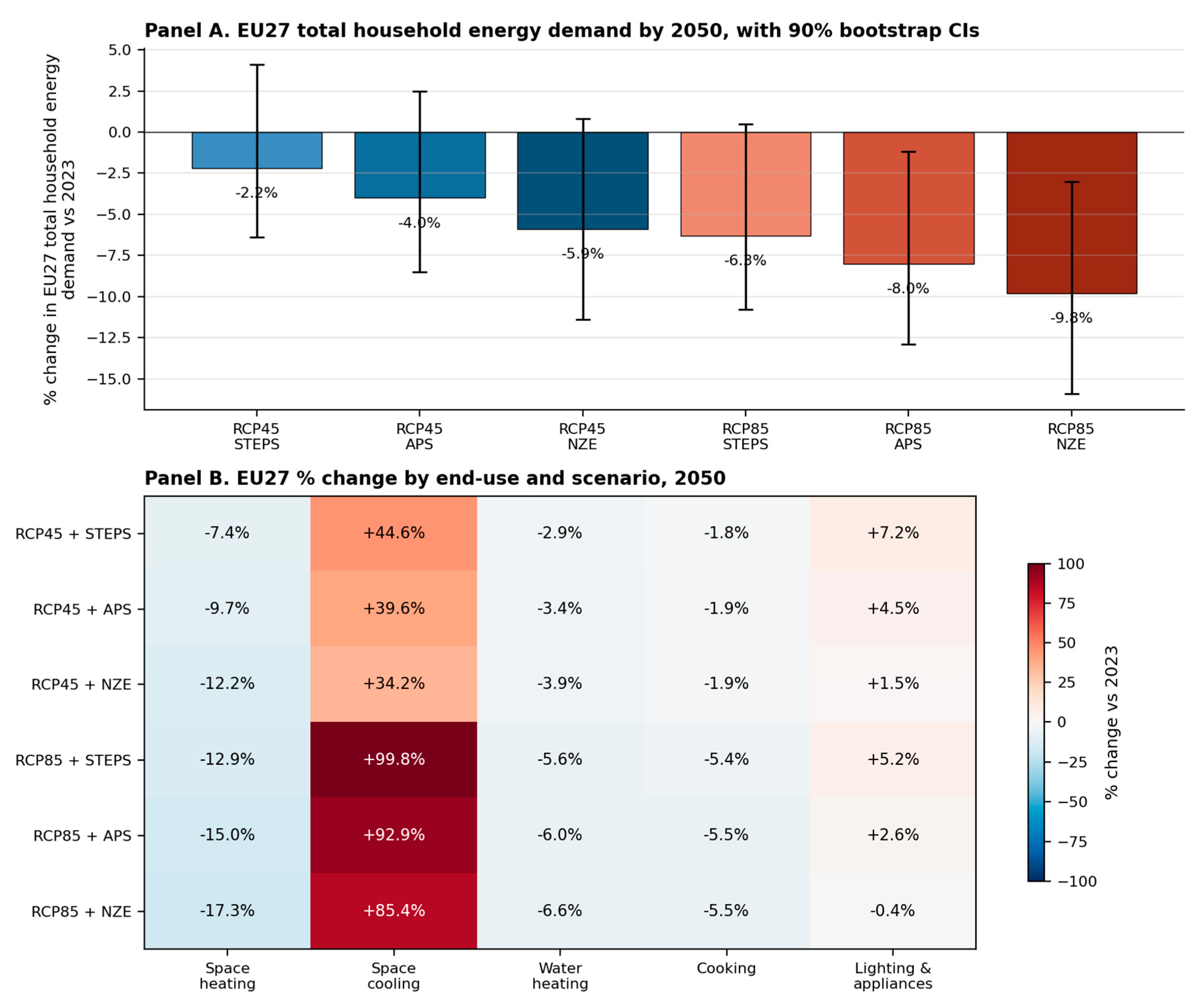
Figure 2.
EU27 household energy demand pathway 2013–2050 under RCP4.5 + APS: historical observations through 2023 and projection to 2050. Panel A shows all end-uses on a linear scale; Panel B shows space heating and space cooling on a log scale to highlight the asymmetric magnitudes.
Figure 2.
EU27 household energy demand pathway 2013–2050 under RCP4.5 + APS: historical observations through 2023 and projection to 2050. Panel A shows all end-uses on a linear scale; Panel B shows space heating and space cooling on a log scale to highlight the asymmetric magnitudes.
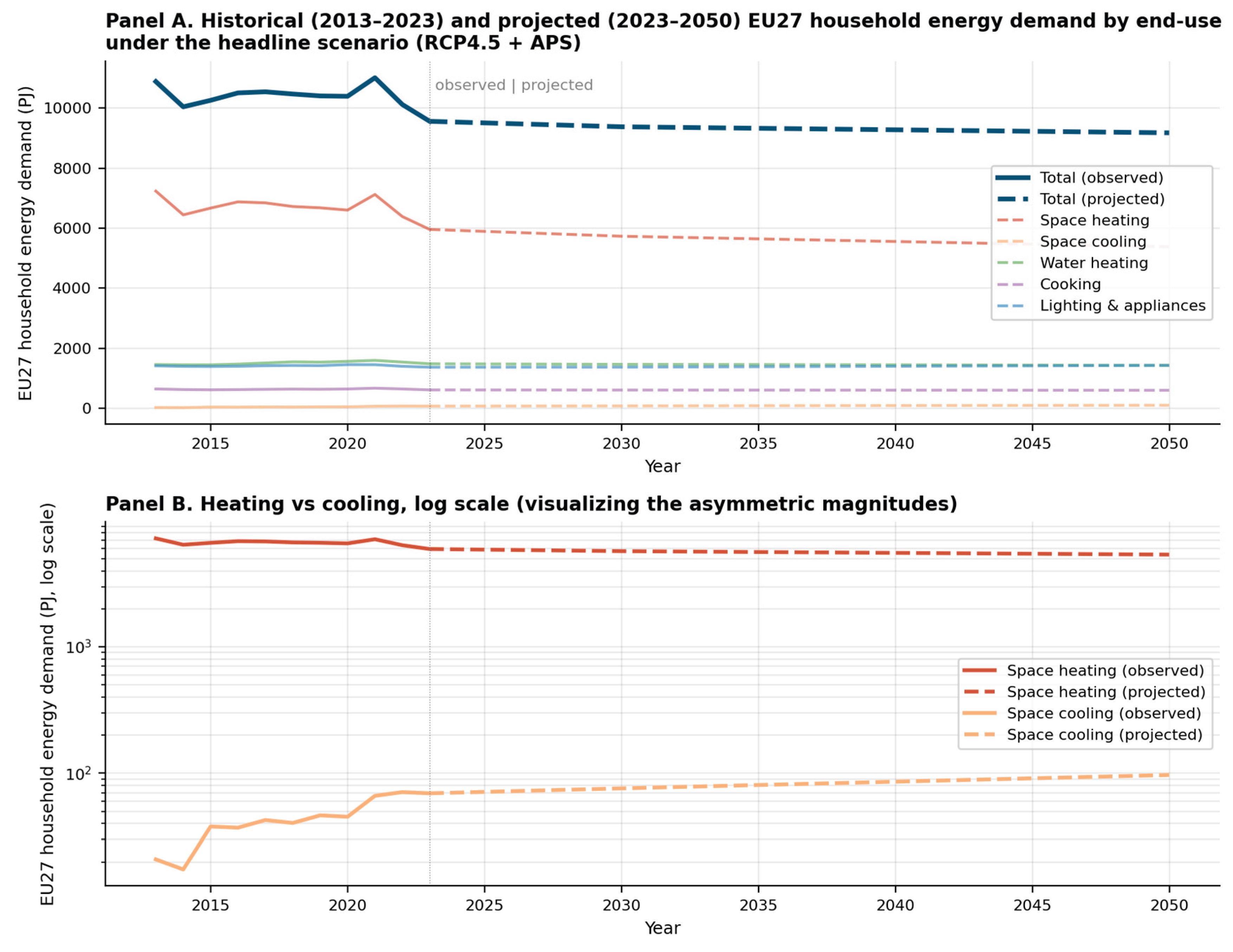
Table 1.
Headline elasticity estimates.
| Regressor | Total | Space heating | Space cooling | Water heating | Cooking | Lighting & appliances |
|---|---|---|---|---|---|---|
| HDD / 1000 | 0.162*** | 0.211*** | 0.144** | 0.085*** | 0.069** | 0.049*** |
| (0.024) | (0.036) | (0.059) | (0.023) | (0.029) | (0.015) | |
| CDD / 1000 | -0.184*** | -0.318*** | 1.951*** | -0.163 | -0.256* | -0.114** |
| (0.039) | (0.100) | (0.419) | (0.099) | (0.136) | (0.046) | |
| log(Real electricity price) | 0.006 | 0.015 | -0.159 | 0.014 | -0.008 | -0.084** |
| (0.027) | (0.032) | (0.107) | (0.041) | (0.048) | (0.039) | |
| log(Real gas price) | -0.085*** | -0.123*** | 0.012 | -0.036** | 0.006 | -0.025 |
| (0.012) | (0.020) | (0.080) | (0.018) | (0.041) | (0.021) | |
| log(Real GDP per capita) | 0.115*** | 0.040 | -0.317 | 0.037 | 0.104 | 0.287*** |
| (0.028) | (0.045) | (0.296) | (0.069) | (0.092) | (0.056) | |
| Time trend | 0.000 | 0.001 | 0.066*** | 0.010*** | 0.002 | -0.002 |
| (0.002) | (0.002) | (0.009) | (0.002) | (0.004) | (0.002) | |
| Observations | 264 | 264 | 173 | 264 | 264 | 264 |
| Countries | 24 | 24 | 17 | 24 | 24 | 24 |
| Within R² | 0.312 | 0.269 | 0.490 | 0.187 | 0.031 | 0.112 |
| Mean of log(E) | 12.24 | 11.76 | 6.71 | 10.29 | 9.23 | 10.23 |
Notes: Log-linear panel regression with country fixed effects and a linear trend, 2013–2023. Driscoll-Kraay standard errors in parentheses (Bartlett kernel, bandwidth = 2). *** p<0.01, ** p<0.05, * p<0.10.
Table 2.
Headline projection.
| End-use | Baseline 2023 (TJ) | Projected 2050 (TJ) | Abs. change (TJ) | % change | 90% CI |
|---|---|---|---|---|---|
| Total | 9,562,901 | 9,179,748 | -383,154 | -4.0% | [-8.5%, +2.5%] |
| Space heating | 5,958,827 | 5,380,073 | -578,753 | -9.7% | [-14.4%, -1.8%] |
| Space cooling | 69,433 | 96,895 | 27,462 | +39.6% | [-5.5%, +145.3%] |
| Water heating | 1,479,542 | 1,429,877 | -49,665 | -3.4% | [-9.3%, +5.3%] |
| Cooking | 608,714 | 597,284 | -11,430 | -1.9% | [-9.7%, +8.1%] |
| Lighting & appliances | 1,364,825 | 1,426,125 | 61,300 | +4.5% | [-10.1%, +20.2%] |
Notes: EU27 household energy demand under RCP4.5 + APS-calibrated medium price by 2050. Pct change point = central estimate; 90% CI from 200 cluster-bootstrap iterations.
Table 3.
Six-scenario projection matrix.
| Climate | Horizon | Aggregate | STEPS (low price) | APS (medium price) | NZE (high price) |
|---|---|---|---|---|---|
| RCP4.5 | 2030 | Direct Total | -0.8% | -1.9% | -2.4% |
| RCP4.5 | 2030 | Sum of end-uses | -1.3% | -2.5% | -3.1% |
| RCP4.5 | 2050 | Direct Total | -2.2% | -4.0% | -5.9% |
| RCP4.5 | 2050 | Sum of end-uses | -3.9% | -5.8% | -7.9% |
| RCP8.5 | 2030 | Direct Total | -2.1% | -3.1% | -3.6% |
| RCP8.5 | 2030 | Sum of end-uses | -2.7% | -3.8% | -4.4% |
| RCP8.5 | 2050 | Direct Total | -6.3% | -8.0% | -9.8% |
| RCP8.5 | 2050 | Sum of end-uses | -7.8% | -9.7% | -11.7% |
Notes: EU27 total household energy demand, % change from 2023. Two aggregates reported: direct estimate from the Total elasticity equation, and sum-of-end-uses estimate aggregated from the five disaggregated projections.
Table 4.
Renovation Wave robustness.
| Envelope efficiency improvement | Space heating % change | Total (sum of end-uses) % |
|---|---|---|
| 0% (no renovation) | -9.7% | -5.8% |
| 20% | -27.8% | -17.2% |
| 40% | -45.8% | -28.5% |
| 60% | -63.9% | -39.9% |
Notes: EU27 demand response by envelope-efficiency improvement. Applied to RCP4.5 + APS + 2050. Because the multiplicative envelope reduction is applied only to space-heating, the Total is reported on the sum-of-end-uses basis (the direct Total equation is not renovation-adjusted and remains at −4.0% across all rows).
Disclaimer/Publisher’s Note: The statements, opinions and data contained in all publications are solely those of the individual author(s) and contributor(s) and not of MDPI and/or the editor(s). MDPI and/or the editor(s) disclaim responsibility for any injury to people or property resulting from any ideas, methods, instructions or products referred to in the content. |
© 2026 by the authors. Licensee MDPI, Basel, Switzerland. This article is an open access article distributed under the terms and conditions of the Creative Commons Attribution (CC BY) license (http://creativecommons.org/licenses/by/4.0/).
Copyright: This open access article is published under a Creative Commons CC BY 4.0 license, which permit the free download, distribution, and reuse, provided that the author and preprint are cited in any reuse.


