

Submitted:
01 July 2026
Posted:
02 July 2026
You are already at the latest version
Abstract
Edge devices are critical components of any Internet of Things (IoT) application that collects data and performs initial processing. Processing often involves classifying a time series for known patterns. Currently, most applications perform classification as quickly and continuously as possible, which is well-suited to real-time use cases. However, continuous processing continuously consumes power. For applications that do not require real-time processing, using multiple processors on a single device can distribute the data collection and processing workload. The key issue with such an architecture is sharing storage for recent data and properly timing the classification process to run periodically. In this paper, a multiplexer-based storage-swapping mechanism is used to reduce energy consumption by recording data in a single storage and sharing it between a continuous, low-power recording processor and a periodic classification processor. Additionally, to further reduce processing, data is stored in segments, which are processed individually. An electronic feature detection (EFD) mechanism is discussed that identifies traits of target patterns using purely electronic components to tag segments of interest for classification. These further lower energy and time-related costs. We use an audio classification problem, augmented with an RC filter as the EFD. This architecture enables the creation of complex prototype devices for initial deployments, which can support multiple machine learning and deep learning models regardless of size, before moving to dedicated commercial devices that use the best-performing models. With this approach, specific models may be chosen in specific contexts to improve accuracy.
Keywords:
Internet of Things
; edge computing
; processors
; time series
; audio classification
; electronic filter
1. Introduction
Edge computing for low-power devices enables data processing closer to the source, reducing latency and bandwidth use [1]. This paradigm is especially valuable for applications such as IoT sensors, wearables, and embedded AI systems, where sending data to the cloud is impractical due to energy or privacy constraints. By minimizing communication with centralized servers, edge computing conserves power and supports real-time responsiveness. Devices such as the Raspberry Pi, ESP32, and ARM Cortex-M microcontrollers are widely used to perform local inference tasks using lightweight AI models [2].
Techniques such as model quantization, pruning, and knowledge distillation help reduce computational loads, enabling AI inference within tight power budgets [3]. Frameworks like TensorFlow Lite and Edge Impulse provide tool chains optimized for deploying neural networks on constrained hardware. Furthermore, edge computing enhances security by keeping sensitive data locally, mitigating risks associated with data transmission. Power-efficient communication protocols, such as LoRa, BLE, and Zigbee, complement edge architectures by enabling low-energy data exchange. In environmental monitoring, predictive maintenance, and smart agriculture, edge devices process signals locally to detect anomalies or trigger actions without relying on the cloud. Ultimately, edge computing enables scalable, intelligent systems that are both energy-aware and latency-sensitive.
The common architecture across all such edge AI applications consists of two tasks: data acquisition and AI prediction or classification. Real-time applications require constant, high-speed monitoring of data; both data acquisition and decision-making must be continuous and real-time. On the other hand, for non-real-time applications, also called asynchronous IoT or opportunistic IoT [4,5], data acquisition must be real-time, but decisions do not have to be. Thus, it is possible to take advantage of this delayed decision-making to reduce power consumption. In this paper, we propose a device design architecture for such non-real-time applications with
- (a)
- Electronic Feature detection to identify and tag certain data that is of interest to the application by electronic means only, e.g., filtering.
- (b)
- Storage switching mechanism to enable swapping data between two processors with a multiplexer for decision-making at specific time periods. This reduces the time during which power consumption is high.
This architecture can support multiple full-scale deep learning models for use on edge devices, e.g., a CNN-based classification algorithm for training and classifying fixed-size segments of a signal. It should be noted that the proposed architecture does not improve data acquisition, which still depends on the microphone’s quality, amplification, and positioning. It simply improves data processing.
2. Related Work
In this section, we discuss current technologies in edge computing platforms and classification on low-power devices. We also discuss various electronic filtering mechanisms in digital signal processing relevant to filter design for the proposed architecture.
2.1. Edge Computations and Architectures
2.1.1. Edge AI
Edge AI on microcontrollers has rapidly advanced due to the development of efficient software frameworks and increasingly capable hardware. Libraries such as TensorFlow Lite for Microcontrollers (TFLM) enable the deployment of machine learning models on devices with kilobytes of RAM by removing dynamic memory allocation and optimizing operators for fixed-point arithmetic [6]. Edge Impulse, another prominent platform, offers a pipeline from dataset acquisition to deployment, supporting real-time signal processing and on-device model inference [7]. CMSIS-NN, developed by ARM, offers highly optimized neural network kernels for Cortex-M devices, thereby improving inference time and reducing memory usage [8]. These frameworks typically support classification models, such as convolutional neural networks (CNNs) and fully connected networks, used for tasks like keyword spotting, motion detection, and gesture recognition [9].
Model compression techniques are crucial for balancing performance and resource constraints in microcontroller-based AI. Quantization is widely used to convert floating-point models into 8-bit integer versions, allowing for significant accuracy loss without compromising deployment on low-memory devices [10]. Pruning and weight clustering further reduce neural network size while maintaining functional accuracy [11]. Knowledge distillation, in which a smaller model learns from a larger, pretrained model, is another strategy to maintain high performance on edge hardware [12]. Real-world applications of these techniques include environmental sound classification, industrial fault detection, and image classification in low-resolution domains [13]. The ability to run AI models directly on microcontrollers expands the scope of intelligent sensing in embedded systems, making them more responsive and context-aware without reliance on cloud processing. Implementing AI at the edge offers notable advantages:
- Reduced Data Transmission: Processing data locally minimizes the need to send large volumes of data to centralized servers, thereby saving energy.
- Lower Latency and Bandwidth Usage: Edge AI enables real-time decision-making without relying on constant cloud connectivity, reducing network strain and associated energy costs.
- Scalability: Efficient edge AI solutions can be scaled across numerous devices without proportionally increasing energy consumption, making them ideal for widespread deployment in industrial applications.
Recent work on edge acoustic sensing shows a clear shift toward compact, low-power, application-specific models rather than large, general-purpose classifiers. Cerutti et al. [14] demonstrated that compact recurrent neural networks can support acoustic event detection on low-energy, low-complexity platforms, while [15] demonstrated the feasibility of deploying acoustic detection algorithms on low-cost, open-source sensors for environmental monitoring. This direction is further supported by [16], who examined energy-efficient audio processing for biologging applications, and by [17], who proposed adaptive animal-borne acoustic monitoring. More domain-specific studies, such as [18] on beehive detection and [19] on duty-cycle recording for bat activity measurement, also indicate that acoustic monitoring systems benefit when the sensing and classification pipeline is adapted to the target sound events, deployment constraints, and energy budget.
Wake-up and event-triggered sensing form a second important strand of this literature. Georgiev et al. [20] showed that smartphone DSP co-processors can support continuous audio sensing more efficiently than relying only on the main processor, while [21] proposed low-power multichannel spectro-temporal feature extraction for audio-pattern wake-up. Gazivoda et al. [22] extended this idea with always-on wake-up detectors for sparse acoustic event detection, in which heavier processing is only activated when potentially relevant acoustic activity is detected. The broader hardware perspective is reinforced by [23] , who surveyed wake-up receivers built from commercial off-the-shelf components, demonstrating that low-power sensing systems can be designed around selective activation rather than continuous full-power operation.
Together, these studies support the proposed use of smaller, specialized acoustic models: instead of running a single large model across all sound classes, a system can use wake-up detection, routing, or context-specific activation to invoke narrower models that may improve accuracy while reducing unnecessary computation.
A critical drawback with most edge devices is the inability to change models as needed. Most platforms require the trained model to be compiled into binary code and installed on the microcontroller. This means that the device’s code is fixed. A high-cost, high-power microcomputer, such as the Raspberry Pi, can be used to load any model as desired; however, it would be severely limited in runtime due to its high power consumption. In the current context, we consider applications that deploy devices to remote regions and must operate continuously to observe the environment and provide near-real-time feedback to humans (but not in real time). Often, the development of such devices is hindered by inaccuracies in models when applied to real-world environments. A new dual-processor architecture could be particularly helpful for testing the accuracy and effectiveness of different models in real-world environments, while maintaining low power consumption and continuous data recording.
2.1.2. Multiple Processors in Edge
Recently, there have been several works that propose edge devices or edge computing platforms that contain multiple processors in the form of heterogeneous SoCs, multi-processor edge nodes, or a combination of CPU/NPU/FPU [24,25], or designs where tasks are partitioned across processors inside a single edge box [26,27,28]. Ref [26,28] focus on reducing the latency that arises when multiple machine learning models run concurrently on the same device. Their work proposes an optimization framework that profiles resource contention—such as CPU load, memory pressure, and I/O delays—and dynamically schedules model execution to minimize end-to-end inference time. But it does not address the power constraints in a practical manner.
Another approach has been a distributed edge AI, which relies on cooperative computation across multiple edge nodes [25,26,28]. These architectures underscore the need for standardized communication frameworks and lightweight coordination protocols to enable heterogeneous devices to operate as a unified intelligence layer. The broader context of heterogeneous edge computing discusses how diverse hardware accelerators—ranging from FPGAs and ASICs to neuromorphic processors—are redefining edge system architecture. It has been argued that no single processor type can meet all edge requirements; instead, optimal performance emerges from the coordinated use of different processing units tailored to specific computational patterns. This suggests the need to develop design principles for scalable, flexible, and reliable heterogeneous edge systems that support real-time workloads.
In this paper, a multiprocessor architecture is proposed in which the workload is shared between a low-power, continuous processor and a relatively high-power, periodically operating processor.
2.2. Edge Power Consumption
Power consumption in edge devices is a critical consideration, especially in remote or mobile deployments. These devices often rely on limited energy sources such as batteries or small-scale solar panels, making power efficiency essential. Solar panels provide a sustainable energy solution, particularly for outdoor deployments such as agricultural sensors or environmental monitoring stations; however, their output is dependent on weather and daylight conditions [29]. Batteries, such as lithium-ion or lithium-thionyl chloride, are commonly used for portable and off-grid applications, with trade-offs between energy density, cost, and rechargeability. Power-efficient hardware platforms, such as ARM Cortex-M processors or ESP32 microcontrollers, are designed to operate in ultra-low-power modes when idle and wake up only when needed. Use-case scenarios vary in their energy demand: for example, periodic sensing and transmission can be optimized to minimize active time, while continuous video or AI inference consumes significantly more power [30]. Therefore, optimizing duty cycles, leveraging hardware sleep states, and using event-triggered processing are crucial strategies for prolonging operational life.
In scenarios where consistent connectivity is unavailable, devices must operate autonomously for extended periods, making efficient energy harvesting and storage vital. In agricultural edge systems, for instance, solar-powered nodes monitor soil moisture or temperature and transmit only critical data to conserve power. On the other hand, wearable health monitors prioritize energy efficiency to prolong battery life while maintaining continuous sensing and local processing. Communication protocols also influence energy usage—LoRaWAN, for example, is ideal for infrequent, long-range communication with minimal power drain. At the same time, Wi-Fi offers higher bandwidth at a much higher energy cost [31]. Advances in low-power AI model deployment, such as TinyML, enable sophisticated local decision-making without significant energy overhead. These models, combined with energy-aware scheduling, allow edge devices to function intelligently within stringent power budgets. As a result, power consumption strategies must be tailored to the specific operational context and environmental constraints of each edge computing scenario.
The most common way to classify is to consider only the last few data points within a fixed time window, as shown in Figure 1. In a continuous, always-on mode, the edge AI would repeat this classification with a gap of 1 ms or less, depending on the application, such as audio classification. For a video- or camera-based application, it may need to process up to 30 frames per second. This continuous process requires significant power, even with an ultra-low-power processor.
This is very useful and necessary for real-time applications, such as keyword spotting. But in remote applications, the data may not be expected to be processed in real time. In this case, classification can be performed in intervals as data is collected continuously.
2.3. Electronics Filtering
Filtering using purely electronic components remains a foundational approach in signal conditioning, particularly in low-power or real-time embedded systems. Analog filters, such as band-pass filters (BPFs), are commonly implemented using resistors, capacitors, and operational amplifiers to isolate desired frequency bands with minimal computational load [32]. Band-pass filters are essential in applications such as audio processing, RF communication, and sensor signal extraction, where specific frequency components must be retained while suppressing unwanted noise. Compared to digital filtering, analog filtering eliminates the need for analog-to-digital conversion, thereby reducing both latency and power consumption, particularly in battery-powered devices [33].
Other alternatives to electronic filters include envelope detectors and differentiators, which extend the functionality of basic filtering by extracting signal dynamics and transient changes. An envelope detector, typically composed of a diode and an RC circuit, captures the amplitude modulation of signals, which is useful for demodulation and audio detection [34]. Differentiator circuits, formed using op-amps and capacitors, respond strongly to sudden changes in the input signal, making them ideal for edge detection or transient analysis. These circuits operate continuously and consume minimal static power, especially when built with low-power op-amps, making them suitable for energy-constrained systems [35]. Together, these analog techniques provide a powerful toolkit for front-end signal processing in embedded and real-time systems without the overhead of digital computation.
In the proposed architecture, electronic feature detection is needed to identify regions of interest, which are then collected and annotated for further classification.
3. Proposed Dual-Processor Architecture
This section discusses the energy-saving principles of the proposed architecture and its key components, including feature detection, storage management, and decision-making.
The target application for the proposed architecture needs to:
- a)
- capture data in real time as part of monitoring
- b)
- Detect events or patterns in the data based on a known set of target patterns or classes
- c)
- Send the list of events to users.
The application does not need a real-time classification. The basic design scheme is shown in Figure 2. For any application requiring real-time monitoring, all data acquisition must be real-time. The data needs to be stored in equal-sized segments. The segment size must be sufficiently small for the AI models to classify it accurately. Classification is performed only periodically by switching storage to the classification module. Because processing a segment takes a short period of time, a large number of segments can be processed in a much shorter time than the total period over which the data was recorded.
To further reduce time, an electronic feature detector is employed to determine whether the incoming signal exhibits a feature expected of a target pattern. If the feature exists in the currently recorded segment, the segment is tagged as containing the feature of interest and subsequently submitted for classification.
3.1. Cost of Classification
3.1.1. Measuring Time and Power Consumption
For edge devices, two key metrics can be evaluated: time and power consumption. This assumes that a fixed dataset is available for training an AI model that can fit within the device’s memory. We consider only non-real-time applications here, focusing on acoustics only. Thus, fast processing is not a priority. Instead, power saving is the key focus here. Below, we define the parameters used to measure the cost of decision-making.
It can be assumed that reducing the time dedicated to inference decisions would reduce power consumption, and vice versa. Power is saved by actually turning off the classification processor and related components of the device, thus preventing it from running at all. If it does not run for a certain period, the power saved is proportional to the time it is switched off. So, the values can be measured in time (e.g., ms) or power (e.g., mW), depending on the platform used. For the rest of the paper, we assume cost as reducing the time for which Processor 2 is ‘on’ and performs the classifications. This way, the cost can be expressed regardless of the actual hardware chosen, which may have different current consumption levels.
To measure either time or power, we define the cost of a decision (or inference) - c. The edge device aims to classify a finite data sample, e.g., a time series or an image, into a specific class. Even in non-real-time applications, data must be collected continuously, but inference need not be real-time. This means that the collected data can be broken down into fixed-size segments of size k, and AI inference (Q) would be performed for each segment.
3.1.2. Minimum Segment Size
One critical parameter to determine before deployment is the minimum data size (k) required for the AI application to achieve accurate classification. In noisy environments, training requires a larger portion of the input data to achieve better results. This means that Q(s) will take a minimal amount of time, but it will not be random, since k is fixed for a given application at a given time. However, the size k of each segment may be adjusted over a longer period, calibrated to specific real-world environments. However, any such change will be gradual, and the classification will be performed on a dataset with equal-sized segments.
For example, in an audio classification scenario, the target sounds are fixed-length (e.g., k = 4 seconds), and the inference determines the sound type for each segment or clip. The net power consumption over a short time period t would be the sum of the costs of all inferences in that period. If all the segments are continuous, then the total cost would be
where L is the initial load time when the classifying components boot up and load the models into memory. This assumes continuous checks of exactly times. Over a long period of time T, before power can be replenished to the device, the total cost of inference becomes
where is a set of clusters of time segments. Each contains a set of continuous segments each of size k. However, and are non-continuous. We term these clusters as segments of interest. Once loaded, the classification of a large number of files or segments is significantly quicker, i.e.,
We present these results in Section 4. For audio applications, the time required to accurately classify a k = 4-second audio clip (segment) is significantly less than 4 seconds, compared to classifying a continuous window. If inference does not occur in real time, no windows are needed, and the segments can be processed in batches much faster. There are two key observations with this approach:
- Assuming that the time gap between each classification bout is δ (which could be in hours), the total cost of a decision for each classification bout would depend on the entire recording period. The net time to process this would be lower than the continuous processing every few milliseconds.
- A cold start problem arises from the need to determine where to start looking, even if the processing time is lower than the time required for data collection. The classifier requires information on where to begin searching for the target pattern. Without this, the scheduler would have to iterate through all the collected information frame by frame or segment by segment. If additional feature information is recorded, then the segments can be tagged, and the clusters T can be formed accordingly.
The following section describes the architecture for obtaining supplementary information in real time using an EFD and for adapting the data processing to the exact time points at which the classifiers should start searching for the target patterns.
3.2. Non-Real-Time Edge Classification Architecture
The Non-Real-Time Edge Classification (NRTC) architecture comprises two processors — a collector and a classifier — and a shared storage system. The collector continuously collects raw data from sensors, such as microphones or cameras. The collector operates at low power and never sleeps (or sleeps only briefly). The classifier is a secondary processor that is more powerful and not restricted by power or memory. Any limitation on the classifier processor is only relative to the actual application. This classifier, however, operates only for a limited time when a large volume of accumulated data is stored in a shared storage system. Because the classifier operates only for a limited time, power consumption peaks briefly. If solar power is available, the power can be restored before the next classification bout. NRTC data processing includes three distinct phases:
- Data Accumulations with Augmentation: Raw data can easily be accumulated by the collector. But suppose the classifier processes all of that data without any supporting information. In that case, the net time and power consumption will still be unnecessarily high, even if the classification time for each segment is significantly shorter.
- Storage Hand-Over: When enough data is accumulated in the shared storage, the collector hands it over to the classifier. This process requires a clean mechanism and supports the required speed and throughput.
- Inference: The secondary classifier processor has significantly more storage available to it. When running the classification algorithm, it can use advanced libraries such as TensorFlow Lite. This would allow it to load multiple models to classify the raw data. The choice of model can be driven by several factors, such as the time of day or additional information collected during the first phase. The ability to invoke multiple models tailored to specific situations on the device enables it to identify multiple target patterns. The decision of which models to use can also be made externally and communicated to the device.
Figure 3 illustrates the NRTC edge architecture, including all its components, as well as the battery and communication modules. Further details of the architecture are discussed in the following few sections. The power of such edge devices can be limited when deployed in remote locations. They may be connected to solar panels or other power sources to recharge the batteries. However, we consider applications where the solar light is not reliably available throughout the day. Hence, there is a need to optimize inference to conserve power while maintaining continuous recording.
3.2.1. Supplementary Information to the Input Signal
To minimize data processing, the collector can record supplementary information alongside the raw data. This can be done computationally, but it would require a more powerful processor and a properly designed algorithm. This will increase both monetary costs and power consumption. In the proposed design, the supplementary information is expected to be determined solely through electronic signal processing, using Electronic Feature Detection (EFD). This module can employ various techniques, including band-pass filters to select a specific frequency range in the input, a tone decoder to detect a particular frequency for a short period, and circuits to detect amplitude bursts or jitter in the signal. It is also vital that the circuit consumes minimal power and produces a clear difference across various conditions, even when supplemented with additional information. As such, the circuit must be configured specifically to target a known pattern.
The supplementary information cannot be expected to classify the raw data correctly; instead, it indicates the region of interest in the timeline. This means the supplementary information is limited and drawn from a predefined list of options. The information can be as small as a single bit — 0 when the supplementary information circuit does not detect anything of interest in the input signal, and 1 when it does. A more complex structure may contain multiple bits that indicate a more complex situation.
For example, in the audio application, we focus on detecting changes in the signal’s amplitude (see Figure 4). This is accomplished using an envelope detector consisting of a diode, capacitor C1, and resistor R1. This captures the high-amplitude component of the input signal. A simple RC filter follows this to determine whether the signal has a nonzero amplitude for a given duration. C2 and R2 are selected to give the collector sufficient time to detect amplitude changes and avoid noise.
Generally, the EFD circuit’s output AUG runs in parallel with the microphone’s direct connection to the recording microcontroller. The AUG is also connected to a pin that can read analog values. The circuit can behave in many ways, such as:
- extended periods () of low non-zero voltage when there is a massive change or burst in the sound level. The RC values can determine the duration of this, depending on the sound environment. This has to be monitored by a dedicated timer on the collector microcontroller. This is a suitable arrangement, as the AUG, while reliable, would have a very low voltage (<500 mV or even <10 mV), which is difficult to detect as a proper interrupt and thus must be polled. This is better for saving power.
- short bursts of HIGH or LOW, which can be attached to a dedicated interrupt. However, for this, an additional layer of amplification is required on the AUG to detect the change at the pin. This should result in an additional power drain and is not suitable for power savings.
Augmented information can be stored alongside the segments. The data primarily identifies which files are most important to start looking for the target patterns. The classifier processor can start with these tagged files and, if necessary, join adjacent files for processing.
In the audio application, the currently recorded filename is simply appended with a 0 or 1, where 1 denotes a file of interest. This is determined by whether the AUG returns a positive result while recording the current file. A 0 indicates that the file, although recorded, only contains background noise. Note that even if the AUG returns a positive result, it only indicates a potential pattern of interest and a target pattern in the file. The stored signal must still be classified into a specific class.
3.2.2. Memory Exchange Between Processors
A critical step in the dual-processor NRTC architecture is the handover of the data for processing. Data is collected continuously in segmented files. Along with the data, the augmented information is stored in the collector processor. The collector processor cannot process this independently. It hands over the entire storage to the classifier processor. The storage capacity is large—measured in GBs—and the number of files could be in the hundreds. The file names are numbered and may include timestamps, allowing the classifier to process the files sequentially. The augmented information indicates to the classifier which files are most likely to contain the target pattern.
The device’s storage is a micro-SD card with more than 4GB of capacity, accessed via SPI. A multiplexer mechanism controlled by the collector processor switches SPI communication lines between the collector processor and the classifier processor. The multiplexer can be implemented using dedicated electronic components, such as a 4x2x1 multiplexer (74HC157) or two bidirectional switches (e.g., CD4066). The normal connection is between the microSD and the collector processor. Storage is handed to the classifier only periodically. When the classifier completes the inferences, the results are computed by the classifier processor and stored on the SD card. Alternatively, the results, once stored on the SD card, can be used by the collector process, which could then communicate. Figure 5 shows this architecture.
One particular issue is that when storage is provided to the classifier, it cannot store any additional data during that period. Although it is expected to run the classification for shorter periods than the recording times, it is still possible to miss critical data. Additionally, it is neither feasible nor easy to reset the storage immediately if EFD detects a positive result on the AUG. Therefore, a pair of shared storage devices may be used, with a second SD card provided to the collector processor for the duration of the classification. Because the collector controls access to the SD cards, it can then hand over the relevant card for classification.
The switch between the processor and SD cards can occur in less than 1 ms, as the controller simply needs to pull up or down the multiplexer’s control pins and activate the classifier processor’s power mechanism. Some specific pins and control lines are needed for communication between the classifier and the collectors:

Table 1.
Dedicated connection lines.
| Line | From | To | Description |
|---|---|---|---|
| IPWR | Collector | Classifier (Power) | This line allows the Collector to enable or disable the classifier’s power input. |
| FIN | Classifier | Collector | This is an input to the Collector that informs it when the Classifier has finished classification. |
| CSW | Collector | MUX | This line enables the Collector to switch the SPI lines connected to the MUX mechanism between the Collector and the classifier. |
Power control to turn the classifier on or off can be implemented using either a Normally Open relay or a MOSFET transistor. Figure 6 shows the basic algorithm running on the collector. The value of can be adjusted using R and C to determine whether the value needs to be tagged.
3.2.3. Decisions by Classifier Processor
Depending on the classifier chosen, classification can be sophisticated or blunt. If a high-performance microcomputer, such as the Raspberry Pi or Jetson Nano, is used, the developer can run Python code that reads from the SD card at boot and processes the files sequentially. Devices like Raspberry Pi consume 500-700 mA during inference and will thus drain significant power from the batteries. However, the Python code can refer to the supplementary information available and select the models correctly. Once the inference is complete, the results will be communicated immediately via a channel such as Wi-Fi or LoRaWAN. A low-power WAN setting is more likely, as a power-starved device is typically deployed in a remote location. Alternatively, a lower-powered device, such as the ESP32, can serve as the classifier, but it will be much more limited in its ability to select multiple and/or larger models. However, it would be a significantly lower overall device cost. In either case, once the decision is made, the pin on the classifier changes state (from LOW to HIGH or vice versa) to indicate to the collector that storage has been released.
The classifier aims to make a decision for each segment stored as a file (e.g., a WAV file) on the storage (e.g., an SD card) as quickly as possible. Decisions are made only for files for which the EFD has detected a feature and tagged. Assuming the target signal occurs only occasionally, the actual period of time required for classification can be significantly reduced.
The example audio application discussed in this paper is built around a deep learning pipeline for environmental sound classification, designed to operate directly on collections of audio files with class labels embedded in the filenames. Each audio clip file is labeled as one of 10 sound classes. After training the model, it is exported in both Keras (h5) and TensorFlow Lite (tflite) formats, enabling deployment on constrained hardware platforms, such as the Raspberry Pi or microcontrollers.
The model size is important here, as large models cannot be loaded onto low-memory microcontrollers, and pruning the model to fit into a small primary memory footprint would reduce accuracy. By swapping the secondary memory and enabling the classifier to access files and the marking feature information, the proposed architecture reduces the model’s size constraints. There may also be multiple models, and a suitable model-selection algorithm can be used.
The algorithm for creating the models may vary in its approach, but it must ultimately follow the basic steps outlined in the flowchart in Figure 7(a). The basic parameters, such as the sampling rate and TFLite models, are required for all applications. For audio, mel-bands and a 4-layer CNN are used in the example scenario presented in his paper, but other applications may employ different mechanisms. The dataset may be the same across multiple training parameter sets, or a range of dataset subsets may be used. For each combination of initial parameters and/or dataset, preprocessing would be applied, potentially with different initial parameters.
The classification process on the classifier is similar, as shown in Figure 7(b). The basic parameters—sampling rate and segment size—are set to the same value, and the classifier processes all files recorded since the last classification. It iteratively processes these signal-segment files to extract the desired signal patterns, then uses TensorFlow Lite to infer the known classification. Because multiple models are available, the classifier can select the appropriate model based on any observation from the premise that meets a predefined criterion, e.g., segment duration or recording time.
One key criterion here is the size of each signal segment, such as an audio clip. The AI algorithm used can accurately detect the correct sound in clips of k = 4 seconds. However, the clip sizes may need to be adjusted to achieve optimal classification performance. This phase of testing is done offline before deploying the models on the device. The benefit of deploying multiple models is that they can be trained for different k values and loaded on demand based on the length or frequency of sound detections in the field.
4. Tests and Results
This section presents the experimental setup and test results of audio classification with a device. The experiments were conducted in a controlled lab environment and aimed to demonstrate the effectiveness of the NRTC architecture in reducing inference time while maintaining high classification accuracy. Figure 8 shows the setup used here. On the left, there is the MAX9814 analog microphone module and the SD card whose SPI pins are connected to the 2 switches (CD4066), each controlled by the Arduino Pro Mini. The microphone is connected directly to the Arduino’s analog pins and via the EFD circuit immediately behind it. The Arduino controls the switches to direct the SD card connection either to itself or to a Raspberry Pi. The relay powers and controls the Raspberry Pi. The collector module, including the microphone, SD card, EFD, and switch, consumes approximately 15 mA continuously when the relay and Raspberry Pi are OFF.
4.1. Electronic Feature Detection
The first component of the device is the filtering or detection mechanism used by the collector module. In this test, we use an audio example and apply a band-pass filter to the microphone input to detect a sound within a specified frequency range. The setup was as shown in Figure 4. The fields are recorded in continuous 4-second clips.
The R1–C1–R2–C2 configuration, with input applied between C2 and R1 and output taken between C1 and R2, forms a passive second-order RC band-pass filter, often referred to as a midpoint RC ring filter or RC bridge network. This circuit exhibits classic band-pass behavior, attenuating both low- and high-frequency components while allowing a defined mid-frequency range to pass through. At low frequencies, the capacitive reactance is high, effectively blocking signal propagation. At high frequencies, the capacitors act as short circuits, shunting the signal and reducing the output amplitude. The output, taken at the midpoint of the loop, captures the frequency band where the impedances of the resistive and capacitive branches are balanced. This structure — also known as a double RC time-constant loop or symmetric RC filter — does not require active components, making it suitable for low-power analog signal conditioning applications, such as transient detection, tone selection, or noise rejection in embedded systems.
The center frequency of this passive RC band-pass filter is determined by the combined time constants of the R1–C1 and R2–C2 branches, typically approximated by
under ideal conditions. The bandwidth and selectivity can be tuned by adjusting the resistor and capacitor values, making the circuit flexible for a range of analog filtering applications. Unlike active filters, this topology requires no power supply or amplification stages, which makes it particularly advantageous in low-power or noise-sensitive environments. The symmetric layout also ensures a balanced response and ease of implementation in both discrete and integrated designs. Moreover, due to its simple structure and predictable frequency response, it serves as a functional building block in audio electronics, communication front ends, and sensor signal preprocessing.
We utilized the UrbanSound8K dataset for our experiments. UrbanSound8K is a widely used environmental audio dataset comprising 8,732 urban sound excerpts, each approximately 4 seconds, collected from field recordings uploaded to the Freesound platform. The dataset comprises 10 distinct sound categories or classes,
facilitating multiclass classification research. To support reproducibility, the audio clips are pre-arranged into ten classes, enabling standardized cross-validation and benchmarking. UrbanSound8K is ideal for training and evaluating deep learning models for real-world sound classification, particularly for applications in smart cities, public safety, and noise monitoring systems.
Two factors determine the EFD module’s success –
- Detection rate: This indicates whether the EFD reliably detects a target sound as soon as it occurs. We test this with two sound levels from a PC speaker. The amplitude threshold was set to 50mV for this configuration.
Disturbance Duration : Depending on the proximity of the sound, the
detected energy would vary, and the EFD would maintain the voltage spike for a
longer period. The duration threshold
was set to 100ms for this configuration.
A segment/file is tagged as ‘of interest’ if, during the recording of that file, the microphone voltage amplitude is above the threshold (50mV), and the amplitude is held for more than 100ms . The distance between the sound source (a
speaker) and the microphone was 0.05m (as clear as possible). Figure 9 shows the results of experiments on the capacitors/resistors from Table 2,
along with the speed at which the EFD detects a sudden frequency burst for each
class in the dataset. In each case, the initial voltage spike is followed by a
de cline
below a threshold, after which the voltage gradually dissipates.
The circuit operates correctly with audio from the MAX9814, which does not supply any negative voltage. The collector, an Arduino Pro Mini 3.3V, captures the initial spike if it exceeds 50 on the ADC (~0.150 V), marking the start of the desired sound. Once detected, the currently recorded file is marked as a potential match for the classifier to investigate.
The sound was recorded at two levels from a computer speaker located 0.1m from the microphone. The sound patterns with a sudden burst are best detected by this EFD, with a detection rate of over 60%. More monotonous, continuous sounds have a lower detection rate. The only exception is dog barking, which has very low sound energy. For the EFD detection test, we added another class – engine_idling (stop) which is done differently from the original engine_idling in the dataset. This was tested by suddenly stopping the engine_idling audio file within 1 s, in which case, its detection rate is very high. The original engine_idling has low detection and is more like background noise. But we don’t use this further, as the original data does not include an audio file for it.
The more interesting characteristic is the duration during which the voltage remains above the threshold. For high-energy sound with a sudden burst, the value on the AUG pin (detected by EFD) remains high for a duration much longer than the clip, but still long enough to be recorded as a segment of interest.
The above results show that the EFD here can clearly distinguish between two sets of sounds. So, we define the sets as (to be classified) and (to be ignored) based on .
The aim now is to identify the sounds from set I and ignore everything from set E. Without the EFD in place, the device would capture all sound, and there would be no mechanism to filter the sounds from E. Thus, without EFD, the sounds that would be put up for classification would be the whole set of recognizable sounds:
Note that in Set A, there are three more sounds - air_conditioning, street_music, and children_playing- but these are background noise and do not appear as an identifiable pattern on the device. With the EFD, the set that would be put up for classification is I = C \ E. We show that, with the EFD and an AI algorithm, confusion about sounds detected in I improves over C.
4.2. Accuracy of Classification Compared to Power Savings
In this section, the AI modeling is discussed. The AI training is not novel, and the architecture enables developers to deploy any model, of any size, as the classifier. It removes all barriers, allowing the developer to focus on model accuracy with respect to the input classes. In this section, we show how to implement a basic training mechanism for the chosen dataset using generative AI, and then demonstrate the advantages of the proposed device architecture by enabling it to choose among multiple models based on the EFD and to swap memory.
4.2.1. Training the AI Model
This work implements a flexible audio classification pipeline for the UrbanSound8K dataset. A model may be trained only on warning- or attention-related sounds, such as gunshots, sirens, car horns, and dog barks, while another model may be trained only on machinery-related sounds, such as jackhammers, drilling, and engine idling. The same training logic can therefore be reused for either full-dataset classification or subset-specific classification.
The training code was generated using artificial intelligence through a one-shot prompt. In this context, one-shot prompting means that the developer provided a single high-level instruction describing the desired dataset, model behavior, hardware condition, output files, and evaluation structure, and the AI system generated a complete executable training script from that instruction. The generated code was then refined interactively to include additional requirements such as stronger augmentation and improved checkpointing. This illustrates how AI-assisted software generation can accelerate experimental machine learning workflows.
The general procedure is summarized in Algorithm 1. The input may be the full set of classes or any selected group of classes. The essential idea is that class selection is treated as a parameter, rather than being hard-coded into the learning method.

The first stage is class-group selection. This is the step that makes the algorithm generic. The developer may define either a single class group, C, containing all classes, or several groups containing selected classes C’. For full UrbanSound8K classification, the group may contain all ten classes. For subset-based classification, the developer may instead define narrower groups. The algorithm does not require any structural change when switching between these cases. Only the group configuration changes.
Once a group is selected, the metadata table is filtered to retain only the audio files belonging to that group. The original dataset class labels are then remapped into local labels. This remapping is necessary because a subset model should not preserve the original ten-class numbering. For example, if a group contains only a car horn, a dog bark, a gunshot, and a siren, these may be remapped to local labels 0, 1, 2, and 3. Similarly, a three-class machinery group may be remapped to local labels 0, 1, and 2. The output layer of the neural network is then created with the same number of units as the current group’s class count.
The preprocessing stage converts raw audio into a fixed input representation suitable for training convolutional neural networks. Each audio file is loaded, converted to mono, resampled to a fixed sampling rate, and forced to a fixed duration. In the implementation, four seconds is used as the standard duration. Shorter clips are padded with zeros, while longer clips are trimmed. This is necessary because neural networks require consistent input shapes within a batch. After waveform standardization, each audio clip is converted into a log-mel spectrogram. The mel spectrogram represents sound energy across perceptually motivated frequency bands over time, while the logarithmic conversion compresses the signal’s dynamic range. This representation is widely used in environmental sound classification because it preserves both temporal and spectral structure.
The spectrogram is then standardized to a fixed shape. In the implemented configuration, the feature tensor has 128 mel bands, 173 time frames, and an additional channel dimension. The resulting input shape is therefore 128 × 173 × 1. Feature values are normalized using the mean and standard deviation of each sample. This per-sample normalization reduces the effect of differences in recording loudness and helps the model learn discriminative spectro-temporal patterns rather than absolute volume differences. To reduce repeated computation, the extracted features are saved into a cache file for each class group. If the same group is trained again, the cache can be loaded directly.
The dataset is then split using the fold structure provided by UrbanSound8K. A fold-based split is preferable to a random split because the dataset contains audio slices that may be related to each other. If random splitting is used, similar slices may appear in both the training and testing sets, leading to overly optimistic performance estimates. In the implementation, folds 1-8 are used for training, fold 9 for validation, and fold 10 for testing. This is approximately an 80:10:10 split by fold count, although the exact file counts may vary because the folds are not perfectly equal in size. The same principle can be generalized to rotating-fold evaluation, where each fold becomes the test fold once, and the final result is reported as the mean performance across folds.
The training pipeline uses TensorFlow datasets. Training data is shuffled and augmented, while validation and test data are left unchanged. Augmentation is applied only during training because validation and testing should measure performance on unmodified held-out data. The implemented augmentation uses a SpecAugment-style approach in which random time regions and frequency regions of the spectrogram are masked. Small Gaussian noise is also added. This encourages the model to learn robust sound patterns rather than memorize exact time-frequency positions. This is especially useful for subset models, where the number of available examples may be much smaller than in the full ten-class problem.
The classifier is a convolutional neural network that treats the log-mel spectrogram as a single-channel image. The model consists of repeated convolutional blocks followed by global average pooling and a dense classification head. Each convolutional block contains convolution layers, batch normalization, ReLU activation, pooling, and dropout. For subset-based classification, the model was deliberately made smaller than the earlier full-capacity version. This is because small class groups can overfit quickly, especially when validation data is limited. A smaller network with stronger dropout and validation-loss checkpointing can often generalize better than a larger model that achieves very high validation accuracy but lower test accuracy.
Class weights are computed for each group using only that group’s training labels. This is important because the class distribution may be uneven. For example, a group may contain many dog bark samples but relatively few gunshot samples. Without class weights, the model may favor the more frequent classes. Class weights increase the training penalty for mistakes on underrepresented classes and reduce the relative dominance of larger classes. However, class weights do not create new data. They only adjust the loss function during training. Their benefit is therefore limited if a rare class has very few or very noisy examples.
Selection of is performed using validation accuracy. Therefore, Algorithm 1 selects the best checkpoint based on validation accuracy and then evaluates the selected model only once on the test fold.
After training, the best model is evaluated on the held-out test set. The evaluation produces both aggregate and detailed results. Aggregate results include test loss and test accuracy. Detailed results include one row per test file, showing the file name, actual class, predicted class, confidence score, and class probabilities. A classification report is also generated, giving precision, recall, and F1-score for each class.
Finally, the trained model is exported for deployment. The implementation saves both the Keras model and TensorFlow Lite versions. A Float32 TFLite model is exported to preserve behavior close to the original Keras model. A dynamic-range-quantized TFLite model is also exported to reduce model size and enable lightweight deployment. This is useful for edge computing scenarios where the model may run on devices such as a Raspberry Pi or other low-power systems. However, the deployment system must reproduce the same preprocessing steps used during training. The input to the exported model must remain a normalized log-mel spectrogram with the same shape, sampling rate, duration, mel-band count, FFT size, and hop length.
For both training and classification, we use the following parameter values, which are suitable for the UrbanSound8K dataset.
The edge inference algorithm loads a trained TFLite acoustic classification model and applies it to WAV files stored in a folder. The class space is first reconstructed by removing the excluded classes, so the model output dimension must match the retained class set C′. Each audio file is converted to mono, resampled, padded or truncated to a fixed duration, and transformed into a normalized log-mel spectrogram suitable for CNN inference. The TFLite model then produces a probability vector , from which the predicted class is selected using argmax and the confidence is taken as the maximum probability. The final output for each file is the predicted retained class label, confidence score, and inference time.
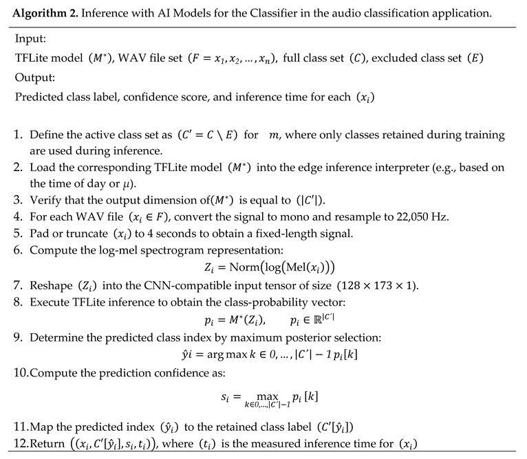
In the current implementation, we use only one model, but based on a selection criterion, a model may be chosen from the classifier’s list of models. For example, using the dataset, two separate models can be trained to predict which sound classes are possible at different times of day. But at least one model should be trained in all the classes.
For the experiment, we played 837 clips from the test data (fold 10) at a distance of 0.01m from the device. This was done to avoid any detection misses and capture all the sound almost as is on the device. This resulted in 837, 4 s clips on the classifier with slightly different sound. All clips were detected, tagged, and added to a single pool of interest (Ω). All of these clips were processed in a single run after all had been played.
4.2.2. Results: Accuracy of Classification
The test results are shown in Figure 10 below. The device had 2 models to choose from, based on the for models , or otherwise use for . In case of , on 289 samples were considered in Ω as the EFD does not flag others.
Model shows strong overall performance, achieving an accuracy of 90.66%, meaning that 262 out of 289 test samples were correctly classified. Most predictions are concentrated on the diagonal of the confusion matrix, with correct classifications of 85 drilling samples, 81 engine_idling samples, and 96 jackhammer samples. The main error pattern is that drilling and engine_idling are sometimes misclassified as jackhammer, while jackhammer is classified perfectly in this test set.
The model achieves an overall accuracy of 78.49%, correctly classifying 657 out of 837 samples. The strongest classes are gun_shot, street_music, car_horn, and jackhammer, with recalls of 100.00%, 95.00%, 93.94%, and 91.67%, respectively. The weakest class is drilling, with a recall of 62.00%, and it is most often confused with jackhammer, with 12 drilling samples predicted as jackhammer. A major source of confusion is between engine_idling and air_conditioner, with 24 engine_idling samples misclassified as air_conditioner. There is also notable overlap between siren and children_playing, with 18 siren samples predicted as children_playing.
We went ahead and ran the test for the excluded sounds E and the recognizable sounds C. The model achieves an overall accuracy of 86.29%, correctly classifying 214 out of 248 samples. The classes car_horn and gun_shot are classified perfectly in this test set, with 33/33 and 32/32 correct predictions, respectively. The dog_bark class also performs strongly, with 91 correct predictions out of 100 samples. The main source of error is the siren class, where 22 siren samples are misclassified as dog_bark, indicating some overlap between these two acoustic patterns.
The model achieves an overall accuracy of 84.17%, correctly classifying 452 out of 537 samples. The strongest class is gun_shot, which is classified perfectly with 32 correct predictions out of 32 samples. The classes car_horn, jackhammer, and engine_idling also perform strongly, with recalls of 93.94%, 92.71%, and 89.25%, respectively. The weakest class is siren, with a recall of 62.65%, mainly because 24 siren samples are misclassified as dog_bark. Another notable error pattern is that drilling is sometimes confused with siren, with 12 drilling samples predicted as siren.
The results suggest that using smaller, specialized models may be more effective than relying on a single model trained on all 10 classes. The full 10-class model achieves an accuracy of 78.49%, which is lower than the smaller models: reaches 90.66%, reaches 86.29%, and reaches 84.17%. This indicates that when the classification problem is restricted to acoustically related or operationally relevant class groups, the model can learn more focused decision boundaries and avoid some of the broader confusion seen in the 10-class setting. This is enabled by using the proposed EFD and dual-processor architecture. With this approach, the device can select over .
Depending on the efficiency of the EFD and the microphone or the incoming signal, overall accuracy may drop, but using a specialized model in specific contexts should yield considerably better performance with the proposed architecture.
4.2.3. Results: Cost of Inference
The key objective of this paper has been to reduce power consumption by shortening the runtime of heavyweight classification tasks. The average load time, L, was 18 seconds for a 10.3 MB model across 4 executions. We also classified 4s, 2s, and 1-second clips, and the average inference time per clip was 160 ms, 104 ms, and 91ms, respectively (see Figure 11). This shows that the time saved by classifying each 4-second clip is exponentially smaller than the clip’s length, and that non-real-time classification saves a huge amount of time on the high-power classifier processor.
The low-power collector module, along with the data acquisition components, draws a continuous current of 15 mA when connected to an Arduino Pro Mini and an analog microphone (MAX9814). This is a manageable consumption with solar power. The Raspberry Pi classifier module consumes approximately 600 mA during execution, which lasted 837 × 160 ms = 134.08 s, thus representing an insignificant burden on the batteries, compared with an always-on configuration, where the total time for the 837 clips would have been 837 × 4 = 3352 seconds. The comparison is shown in Table 4 below.
With a single-processor, always-on configuration, incoming data is buffered into segments lasting a few milliseconds before being classified. For this, the training dataset also needs an ‘other/none’ class, which would just be background noise. This is not present in the UrbanSound8K, but given the accuracy achieved with various real-time systems [36,37], an accuracy of over 90% can be achieved for this case as well. However, the size of such a model is not guaranteed to be small enough to easily fit into a constrained IoT edge device. Also, choosing a better segment size could improve accuracy.
The net cost of inference is mentioned in time, as a different choice of classifier process would lead to different real power consumption.
4.2.4. Power Characteristics
Regarding a power-consumption benchmark, we consider a system that consumes the least power over the longest duration. To achieve perpetual operation with a 5V battery, assuming a 5W solar panel operating under 5 peak sun hours per day with 75% system efficiency, the maximum current consumption is ~156.25 mA. The daily harvested energy is approximately 5 × 5 × 0.75 = 18.75 Wh.
At 15 mA, the collector module current is much lower than 156 mA, so the recording can continue indefinitely, assuming no further amplification is needed. If the Raspberry Pi is OFF for more than the recording’s net time, the power consumed for classification can be considered negligible and can be replenished quickly by solar power.
5. Discussions
In this section, we discuss the limitations, advantages, and future work.
5.1. Limitations and Future Work
Aside from reducing the time for critical power-consuming processes, the proposed architecture inherits other issues with edge AI, particularly the noise factor, i.e., what happens when a sound appears that is not in the trained classes. While multiple models and the EFD may provide better decisions, they may still not be perfect.
The key future improvement needed is a uniform AI modeling strategy across all data segments. This was easy with the dataset used, as the data were collected methodically and the target sounds occurred reliably within the recorded clips. Although the sound lengths in the clips varied widely, the files were still recorded with the same energy, providing some uniformity. However, a dataset with significant time variations in the target sound may make it difficult to train an AI model using Algorithm 1. Thus, it is necessary to choose the right clip size.
Obviously, the more classes there are, the more difficult it is to select these parameters, as shown in Table 3. However, this can be addressed by using multiple data subsets with external features (e.g., time of day) to train dedicated models and by cascading a set of AI models to assign a class to a segment. Some of the deciding factors for choosing an onboard AI model could be:
- (a)
- environmental conditions as determined by additional onboard sensors. For example, it’s a rainy day or a sunny day.
- (b)
- External communication and changing the settings through remote control
- (c)
- Time factors, e.g., time of day, day in calendar, time elapsed since any known event has passed.
Ultimately, these could lead to changes to the selected model(s) based on a set of factors at a given point in time.
Another area to improve is the size of the segment (k). In this paper, we used the value of k from the dataset itself to more easily align training with the clip sizes. The processing time decreases as k decreases, but the relationship between k and model accuracy warrants further investigation.
5.2. Key Advantages of the Multi-Processor Architecture
The main advantage of the proposed method is that it can significantly reduce the high-power execution time required for data classification on an edge device. It should allow the device to use multiple models for data classification. Apart from the obvious advantages laid out in Section 3, the other advantages are:
- (a)
- Prototyping: A key advantage of the architecture is the removal of the size limits of the AI models. It is often a tedious process to create an AI model that is both accurate and small enough to fit in devices’ memory. Also, it is most often just one model on a single processor. In the proposed architecture, multiple models can be loaded and selected according to a controlled strategy. This is very useful during the prototyping phases of development, where the device can first be tested for practicality in the target environment, allowing the AI models to be further optimized at a later stage.
- (b)
- Scalability: We discussed a dual-processor mechanism in this paper and considered only one kind of data. It can be scaled to include 1 or 2 storage devices being switched among multiple processors. Only the processor would collect the data, while the others would run classification individually. This would allow for parallel classifications. The proposed scheme would be effective as long as the total length of segments from the start of the last classification round (δ), or the sum of all segment lengths of the current Ω, is less than or more than the product of the number of processors (n), the number of segments in Ω, and the average inference time, i.e.,
If using the EFD,
Or if not using EFD,
(c) The modular design allows the user to replace the classifier. However, currently only devices classified as microcomputers, such as the Raspberry Pi and BeagleBone, can perform this role because they have sufficient RAM to load the models. This works to the developers’ advantage, as they can ignore model size and train the model to achieve the best accuracy. As microcontrollers are poised to have better RAM, they can eventually load larger models. It is worth noting that with the data used in this paper (Urbansound), it would be difficult, if not impossible, to build a TFLite model under 1 MB, as required by microcontrollers. Hence, for such applications, this device design can reduce power consumption while maintaining performance at a slightly higher per-device cost until more advanced microcontrollers become available.
The EFD used in this paper is a static circuit. However, future designs can be made adaptable to reduce missed detections, as shown in Figure 7(a).
6. Conclusions
Sharing the workload between processors on a single edge device can reduce processing time. By separating the core aspects of an edge device’s functionalities - recording and classification, the device can perform the functionalities at different paces as required. Additionally, using an additional electron-filtering mechanism to identify a specific segment, and then, if the data contains the target patterns, focusing processing on those segments only further reduces processing time.
Author Contributions
Conceptualization, A.M.; methodology, A.M.; software, A.M.; validation, A.M.; formal analysis, A.M.; investigation, A.M.; resources, A.M.; data curation, A.M.; writing—original draft preparation, A.M.; writing—review and editing, A.M.; visualization, A.M.; All authors have read and agreed to the published version of the manuscript.
Funding
This research received no external funding.
Data Availability Statement
The dataset used in this study is publicly available on Kaggle at https://www.kaggle.com/datasets/chrisfilo/urbansound8k.
Conflicts of Interest
The authors declare no conflicts of interest.
Abbreviations
The following abbreviations are used in this manuscript:
| EFD | Electronics Feature Detection |
| NRTC | Non-Real-Time Classification |
References
- Shi, W.; Cao, J.; Zhang, Q.; Li, Y.; Xu, L. Edge Computing: Vision and Challenges. IEEE Internet Things J. 2016, 3, 637–646. [Google Scholar] [CrossRef]
- Chen, J.; Ran, X. Deep Learning With Edge Computing: A Review. Proc. IEEE 2019, 107, 1655–1674. [Google Scholar] [CrossRef]
- Han, S.; Pool, J.; Tran, J.; Dally, W. Learning both weights and connections for efficient neural network. Adv. Neural Inf. Process. Syst. 2015, 28. [Google Scholar]
- Teixeira, R.C.M.; Carvalho, C.B.; Calafate, C.T.; Mota, E.; Fernandes, R.A.; Printes, A.L.; Nascimento, L.B.F. FloatingBlue: A Delay Tolerant Networks-Enabled Internet of Things Architecture for Remote Areas Combining Data Mules and Low Power Communications. Sensors 2024, 24. [Google Scholar] [CrossRef] [PubMed]
- Madamori, O.; Max-Onakpoya, E.; Erhardt, G.D.; Baker, C.E. Enabling Opportunistic Low-cost Smart Cities By Using Tactical Edge Node Placement. Proceedings of the 2021 16th Annual Conference on Wireless On-demand Network Systems and Services Conference (WONS) 2021, 2021, 1–8. [Google Scholar] [CrossRef]
- David, R.; Duke, J.; Jain, A.; Janapa Reddi, V.; Jeffries, N.; Li, J.; Kreeger, N.; Nappier, I.; Natraj, M.; Wang, T. Tensorflow lite micro: Embedded machine learning for tinyml systems. Proc. Mach. Learn. Syst. 2021, 3, 800–811. [Google Scholar]
- Hymel, S.; Banbury, C.R.; Situnayake, D.; Elium, A.; Ward, C.; Kelcey, M.; Baaijens, M.; Majchrzycki, M.; Plunkett, J.; Tischler, D.; et al. Edge Impulse: An MLOps Platform for Tiny Machine Learning. ArXiv 2022, abs/2212.03332. [Google Scholar]
- Lai, L.; Suda, N.; Chandra, V. CMSIS-NN: Efficient Neural Network Kernels for Arm Cortex-M CPUs. 2018. [Google Scholar] [PubMed]
- Warden, P.; Situnayake, D. TinyML: Machine Learning with TensorFlow Lite on Arduino and Ultra-low-power Microcontrollers; O’Reilly, 2020. [Google Scholar]
- Jacob, B.; Kligys, S.; Chen, B.; Zhu, M.; Tang, M.; Howard, A.; Adam, H.; Kalenichenko, D. Quantization and Training of Neural Networks for Efficient Integer-Arithmetic-Only Inference. In Proceedings of the 2018 IEEE/CVF Conference on Computer Vision and Pattern Recognition, 18-23 June 2018, 2018; pp. 2704–2713. [Google Scholar]
- Han, S.; Pool, J.; Tran, J.; Dally, W.J. Learning both weights and connections for efficient neural networks. In Proceedings of the Proceedings of the 29th International Conference on Neural Information Processing Systems -, Montreal, Canada, 2015; Volume 1, pp. 1135–1143. [Google Scholar]
- Hinton, G.E.; Vinyals, O.; Dean, J. Distilling the Knowledge in a Neural Network. ArXiv 2015, abs/1503.02531. [Google Scholar]
- Banbury, C.; Zhou, C.; Fedorov, I.; Matas, R.; Thakker, U.; Gope, D.; Janapa Reddi, V.; Mattina, M.; Whatmough, P. Micronets: Neural network architectures for deploying tinyml applications on commodity microcontrollers. Proc. Mach. Learn. Syst. 2021, 3, 517–532. [Google Scholar]
- Cerutti, G.; Prasad, R.; Brutti, A.; Farella, E. Compact recurrent neural networks for acoustic event detection on low-energy low-complexity platforms. IEEE J. Sel. Top. Signal Process. 2020, 14, 654–664. [Google Scholar]
- Prince, P.; Hill, A.; Piña Covarrubias, E.; Doncaster, P.; Snaddon, J.L.; Rogers, A. Deploying Acoustic Detection Algorithms on Low-Cost, Open-Source Acoustic Sensors for Environmental Monitoring. Sensors 2019, 19, 553. [Google Scholar] [CrossRef] [PubMed]
- Miquel, J.; Latorre, L.; Chamaillé-Jammes, S. Energy-Efficient Audio Processing at the Edge for Biologging Applications. J. Low. Power Electron. Appl. 2023, 13, 30. [Google Scholar] [CrossRef]
- Jean, D.; Turner, J.; Hedgecock, W.; Kalmár, G.; Wittemyer, G.; Lédeczi, Á. Animal-Borne Adaptive Acoustic Monitoring. J. Sens. Actuator Netw. 2025, 14, 66. [Google Scholar] [CrossRef]
- Sad, C.; Kampelopoulos, D.; Sofianidis, I.; Kanelis, D.; Nikolaidis, S.; Tananaki, C.; Siozios, K. Deep Edge IoT for Acoustic Detection of Queenless Beehives. Electronics 2025, 14, 2959. [Google Scholar] [CrossRef]
- Krishna, A.; Lee, W.-J. Influ. Duty-Cycle Rec. Meas. Bat Act. Passiv. Acoust. Monit. 2025. [CrossRef]
- Georgiev, P.; Lane, N.D.; Rachuri, K.K.; Mascolo, C. Dsp. ear: Leveraging co-processor support for continuous audio sensing on smartphones. In Proceedings of the Proceedings of the 12th ACM Conference on Embedded Network Sensor Systems, 2014; pp. 295–309. [Google Scholar]
- Oletic, D.; Bilas, V.; Magno, M.; Felber, N.; Benini, L. Low-power multichannel spectro-temporal feature extraction circuit for audio pattern wake-up. In Proceedings of the Proceedings of the 2016 Conference on Design, Automation & Test in Europe, Dresden, Germany, 2016; pp. 355–360. [Google Scholar]
- Gazivoda, M.; Oletić, D.; Bilas, V. Features and Always-On Wake-Up Detectors for Sparse Acoustic Event Detection. Electronics 2022, 11, 478. [Google Scholar] [CrossRef]
- Fromm, R.; Kanoun, O.; Derbel, F. Wake-Up Receivers Based on Commercial Off-the-Shelf Components: A Survey. IEEE J. Microwaves 2026, 6, 42–80. [Google Scholar] [CrossRef]
- Byers, C. Heterogeneous Computing in the Edge. Ind. Internet Consort. 2021. [Google Scholar]
- Zao, J.; Byers, C.; Murphy, B.; AbiEzzi, S.; Banks, D.; An, K.; Michaud, F.; Bartfai-Walcott, K. The industrial internet of things distributed computing in the edge; 2020. [Google Scholar]
- Li, P.; Wang, X.; Huang, K.; Huang, Y.; Li, S.; Iqbal, M. Multi-Model Running Latency Optimization in an Edge Computing Paradigm. Sensors 2022, 22, 6097. [Google Scholar] [CrossRef] [PubMed]
- Hu, F.; Mehta, K.; Mishra, S.; AlMutawa, M. Distributed Edge AI Systems. In Proceedings of the Proceedings of the 16th IEEE/ACM International Conference on Utility and Cloud Computing, Taormina (Messina), Italy, 2024; p. Article 56. [Google Scholar]
- Liu, Y.; Qu, H.; Chen, S.; Feng, X. Energy efficient task scheduling for heterogeneous multicore processors in edge computing. Sci. Rep. 2025, 15, 11819. [Google Scholar] [CrossRef] [PubMed]
- Taneja, J.; Jeong, J.; Culler, D. Design, Modeling, and Capacity Planning for Micro-solar Power Sensor Networks. In Proceedings of the 2008 International Conference on Information Processing in Sensor Networks (ipsn 2008), 22-24 April 2008, 2008; pp. 407–418. [Google Scholar]
- Somvanshi, S.; Islam, M.M.; Chhetri, G.; Chakraborty, R.; Mimi, M.S.; Shuvo, S.A.; Islam, K.S.; Javed, S.; Rafat, S.A.; Dutta, A. From tiny machine learning to tiny deep learning: A survey. ACM Computing Surveys, 2025. [Google Scholar]
- Raza, U.; Kulkarni, P.; Sooriyabandara, M. Low Power Wide Area Networks: An Overview. IEEE Commun. Surv. Tutor. 2017, 19, 855–873. [Google Scholar] [CrossRef]
- Sedra, A.S.; Smith, K.C.; Carusone, T.C.; Gaudet, V. Microelectronic Circuits; Oxford University Press, 2020. [Google Scholar]
- Franco, S. Design with Operational Amplifiers and Analog Integrated Circuits; McGraw-Hill, 1988. [Google Scholar]
- Horowitz, P.; Hill, W. The Art of Electronics; Cambridge University Press, 2015. [Google Scholar]
- Nilsson, J.W.; Riedel, S.A. Electric Circuits; Prentice Hall, 2011. [Google Scholar]
- Arik, S.O.; Kliegl, M.; Child, R.; Hestness, J.; Gibiansky, A.; Fougner, C.; Prenger, R.; Coates, A. Convolutional recurrent neural networks for small-footprint keyword spotting. arXiv 2017, arXiv:1703.05390. [Google Scholar]
- Kim, B.; Chang, S.; Lee, J.; Sung, D. Broadcasted residual learning for efficient keyword spotting. arXiv 2021, arXiv:2106.04140. [Google Scholar]
Figure 1.
A time sliding-window based classification for real-time audio classification. Each window is the same size, and the fixed-size time series data is processed in real time as it is received.
Figure 1.
A time sliding-window based classification for real-time audio classification. Each window is the same size, and the fixed-size time series data is processed in real time as it is received.
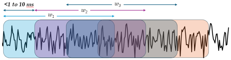
Figure 2.
The dual-processor design.

Figure 3.
The overall device architecture.
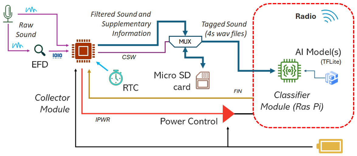
Figure 4.
The electronic feature detection circuit includes an RC network that filters sudden changes in sound amplitude. This is an example circuit used in the experimentation below. The augmentation circuit can be configured according to the application.
Figure 4.
The electronic feature detection circuit includes an RC network that filters sudden changes in sound amplitude. This is an example circuit used in the experimentation below. The augmentation circuit can be configured according to the application.

Figure 5.
The HAND-OVER process between the collector and classifier.
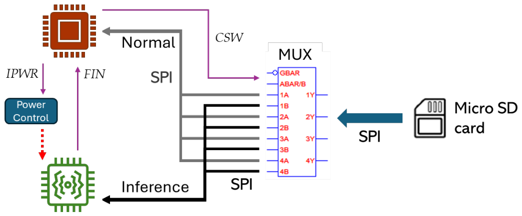
Figure 6.
The algorithm running on the collector.
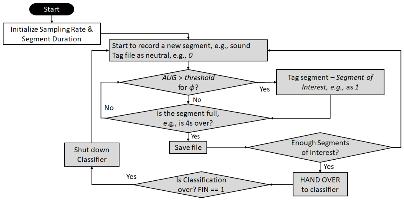
Figure 7.
The algorithms for (a) training a model for classification; (b) classification on the classifier after HAND OVER.
Figure 7.
The algorithms for (a) training a model for classification; (b) classification on the classifier after HAND OVER.
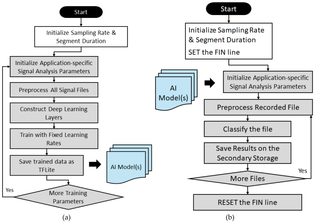
Figure 8.
The basic circuit for DAQ, storage switching, and the collector processor, along with an NO relay for the Raspberry Pi 3 B.
Figure 8.
The basic circuit for DAQ, storage switching, and the collector processor, along with an NO relay for the Raspberry Pi 3 B.
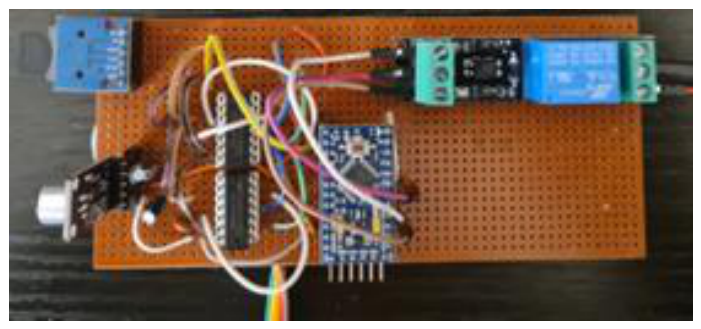
Figure 9.
Electronic Feature Detection performance (a) detection rate of the segment of interest, i.e., the voltage detected by EFD when above threshold for at least 100ms continuously, (b) duration of the voltage above threshold for each sound pattern.
Figure 9.
Electronic Feature Detection performance (a) detection rate of the segment of interest, i.e., the voltage detected by EFD when above threshold for at least 100ms continuously, (b) duration of the voltage above threshold for each sound pattern.
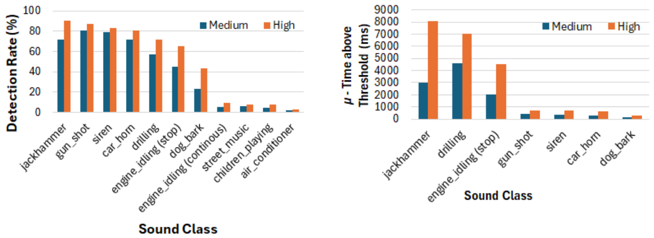
Figure 10.
Confusion Matrix for each model.
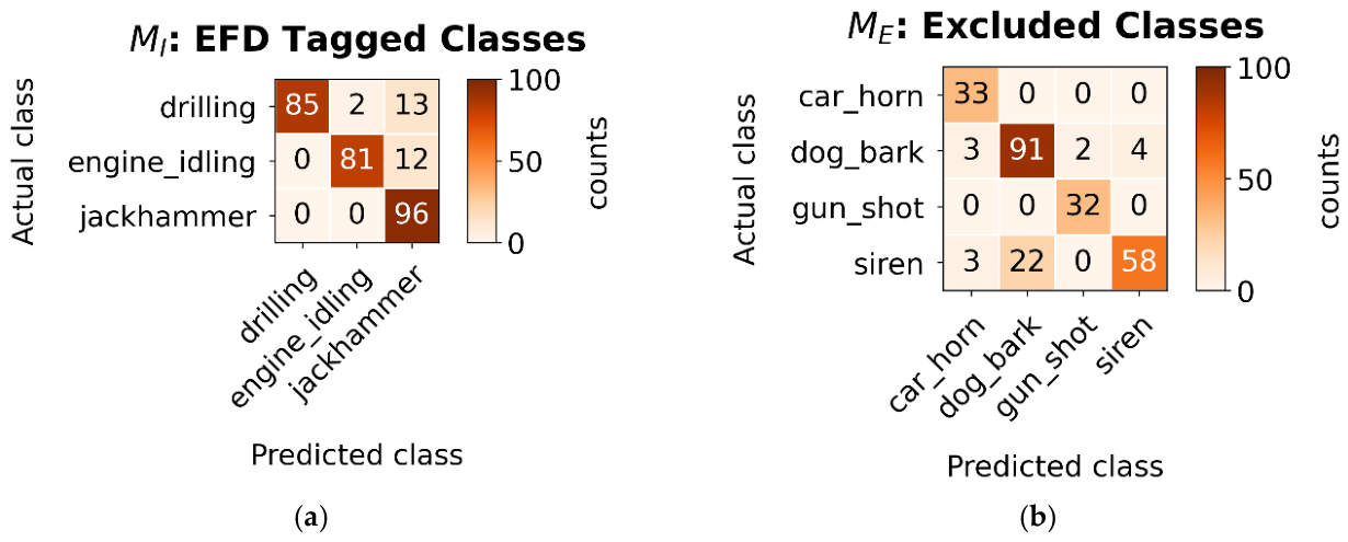
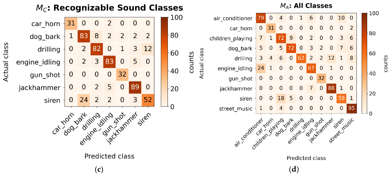
Figure 11.
The time cost varies with the segment’s size.
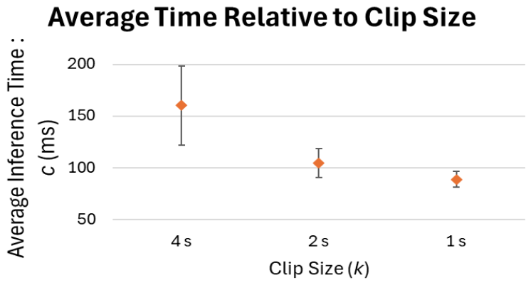
Table 2.
Values of electronic components for the RCRC band-pass filter.
| Component | Value |
|---|---|
| R1 R2 C1 C2 C3 |
22 kΩ 10 kΩ 1μF 4.7 μF 1 nF |
Table 3.
Values of Deep Learning Parameters for Algorithm 1.
| Parameter | Value |
|---|---|
| Sampling Rate: Clip duration: k Mel-Band |
22050 Hz 4 s 128 |
Table 4.
Performance comparison of Classification with different configurations.
| Configuration | Net cost of inference |
Accuracy | Ω |
|---|---|---|---|
| Single Processor Always-on | 3352 s | ≥ 90% * | - |
| Proposed Architecture without EFD | 134.08 s | 78.49% | 837 |
| Proposed Architecture with EFD set for I | 46.24 s | 90.66% | 289 |
*estimation based on literature.
Disclaimer/Publisher’s Note: The statements, opinions and data contained in all publications are solely those of the individual author(s) and contributor(s) and not of MDPI and/or the editor(s). MDPI and/or the editor(s) disclaim responsibility for any injury to people or property resulting from any ideas, methods, instructions or products referred to in the content. |
© 2026 by the author. Licensee MDPI, Basel, Switzerland. This article is an open access article distributed under the terms and conditions of the Creative Commons Attribution (CC BY) license.
Copyright: This open access article is published under a Creative Commons CC BY 4.0 license, which permit the free download, distribution, and reuse, provided that the author and preprint are cited in any reuse.


