

Submitted:
26 June 2026
Posted:
02 July 2026
You are already at the latest version
Abstract
Photovoltaic (PV) backsheets are subjected to continuous environmental stressors, resulting in gradual tensile strength degradation and reduced long-term module reliability. This paper presents a six-stage statistical modeling framework to quantify how cumulative ultraviolet (UV) exposure, temperature, relative humidity, and wind speed each contribute to tensile strength loss in a multilayer PPE-based PV backsheet (polyethylene terephthalate/polyethylene terephthalate/ethylene vinyl acetate, PET/PET/EVA). Pearson correlation using a field dataset of 511 sequential observations of cumulative UV doses (0.84 MJ/m² to 271.6 MJ/m²) established UV irradiance as the most important degradation driver (r = -0.960, R² = 0.921). Since the observations constitute one degradation time series, the serial autocorrelation was checked with the Durbin-Watson statistic and confirmed, necessitating Newey-West heteroscedasticity and autocorrelation-consistent (HAC) standard errors in all the inferential tests. Following a HAC correction, cumulative UV is the strongest predictor. The rate of tensile strength degradation with respect to cumulative UV exposure was estimated at 0.21–0.22 MPa per MJ/m², based on ordinary least squares (OLS), multiple regression, and weighted least squares (WLS) models applied following the Breusch–Pagan test for heteroscedasticity. The second-order regression model gave a better predictive performance with R² = 0.9686 and RMSE = 3.033 MPa; six of the nine higher-order terms were found significant after HAC correction, whereas the UV Temperature interaction became insignificant, which demonstrates the practical effect of the autocorrelation correction. Weibull distribution fitting was the best performer with shape parameter β = 15.87 and B10 tensile strength threshold of 193.14 MPa at approximately 15.4 years of field exposure. Cost benefit analysis showed that premium fluoropolymer backsheets had a net present value benefit of about $7.55 per module in comparison to 25-year design life. These results provide a model of PV backsheet degradation, which can be easily reproduced, and which can be directly applied to reliability-based design and cost-effective lifecycle models.
Keywords:
photovoltaic backsheet
; tensile strength degradation
; second-order polynomial regression
; weighted least squares
; Newey-West HAC
; serial autocorrelation
; Weibull reliability
; UV exposure
1. Introduction
Having a photovoltaic module to work consistently over 25 to 30 years is not merely an engineering dream, it is a guarantee that is required by the contract in most project financiers (Lv et al., 2020; Al Mahdi et al., 2023). The backsheet is often not given serious consideration as one of the elements with the highest long-term mechanical risk. It has three functions, to conduct electrical protection against high-voltage fields, to provide mechanical protection to the interior cell assembly, and to provide a moisture and chemical barrier at the exposed rear side of the module. Once the backsheet starts to degenerate, the module will also degenerate, and the degeneration process is usually irreversible.
The laminate type of PPE is built by applying a white-colored polyethylene terephthalate (WPET) outermost layer on the cell side, clear polyethylene terephthalate (PET) core, and EVA inner layer at the interface with the air. The three-layered structure is commercially common due to the mechanical support that is offered by PET: tensile strength, dimensional stability, and breakdown at electricity (Lin et al., 2016; Kempe et al., 2021). The EVA coating guarantees compliance of adhesive with the module encapsulant. Both are degraded in ultraviolet light, facilitating the chain scission and carbonyl group formation in the polymer backbone and steadily reducing the tensile strength and encouraging surface cracking (Damo et al., 2023; Zhang et al., 2022).
The cumulative UV irradiance is the most common driver of mechanical degradation in PET-based backsheets, followed by the temperature and relative humidity as secondary stressors, which interact with each other (Field and lab aging studies). The technical difficulty of converting such a qualitative insight into a validated quantitative model is more challenging than it may seem since multilayer degradation is spatially heterogeneous, the relationships between stressors and responses are nonlinear and interactive, and the measurement variance increases with the accumulation of UV (Mitterhofer et al., 2024; Smith et al., 2023).
The predictive accuracy is not enough in an industrial and systems engineering perspective. The model must also be statistically defensible: violations fixed, and inference made with reasonable grounds. Second-order polynomial regression is effectively proven to describe the primary effects and an interaction between multiple environmental factors (Chen et al., 2025). Two statistical complications are taken directly in this paper. First, the OLS residuals are tested using the Breusch-Pagan test which identifies heteroscedasticity and then is corrected using the weighted least squares (WLS). Second, and more importantly, the 511 observations are obtained in one sequence of degradation trace, but not measurements of several specimens. The Durbin-Watson statistic is thus used to test serial autocorrelation and correct the whole procedure with Newey-West HAC standard errors (Kuman, 2023), that deal with both conditions of heteroscedasticity and autocorrelation and give valid results in either scenario. The degradation model is then converted into practical estimates of failure probability through statistical reliability analysis (Li et al., 2020; Shama et al., 2023).
These are the six stages of the analysis through which this paper makes its contribution: (1) Pearson correlation to rank the importance of stressors; (2) OLS regression with full ANOVA; (3) Breusch-Pagan and Durbin-Watson testing with WLS and Newey-West HAC corrections; (4) the second-order regression of the nonlinear and interaction effects and HAC corrected inference; (5) Weibull versus lognormal distribution comparison by AIC, BIC, and KS; and (6) a cost benefit analysis with a discounted payoff using a 25-year design horizon comparing the premium strategy and the standard backsheet strategy.
2. Literature Review
2.1. Mechanical Degradation of PV Backsheet Polymers
Tensile strength is the most operationally relevant mechanical property to determine the reliability of backsheet since it defines the limit between the laminates that can support field loads and those that cannot (Zhang et al., 2022; Markert et al., 2024). The location of this threshold depends on the exact composition of the layer and history of its processing, which is also supported by mechanical characterization research of PV encapsulation polymers (Gaddam et al., 2021). Three intersecting degradation pathways (photo-oxidation of UV, chain scission through moisture, and crystallization in amorphous domains of polymer under heat) diminish tensile strength due to outdoor exposure (Lin et al., 2016; Kempe et al., 2021).
One of the most detailed descriptions of such degradation process in commercial PPE backsheets has been provided by Lin et al. (2016), who combined 510 days of outdoor aging at Gaithersburg, Maryland, and NIST SPHERE accelerated laboratory exposure. Tensile strength and break elongation reduced by 26.7% during the same period and surface cracking appeared between days 125 and 184. Tests of mode I fracture toughness (KIc) gave a value of 0.03 to 0.12 MPa·m½ on tests of channel-cracking fragmentation on WPET outer layer, which is significantly lower than the 4.5 to 5.5 MPa·m½ in tests of unaged PET. Notably, the experiment revealed that rapid exposure to UV (acceleration) recapitulated the patterns of the field damage, thus approving cumulative UV dose to serve as a useful proxy of a field exposure time in a sequence of degradation records.
Lv et al. (2020) used the field data of multiple sites to verify that UV irradiance always makes a prevailing difference when predicting mechanical property degradation in various climatic areas. Mitterhofer et al. (2024) have performed a hybrid of finite-element simulation and fragmentation testing and concluded that the severity of the crack in AAA and PPE backsheets is strongly dependent on the properties of the adhesive layer at the interfaces of PET. Smith et al. (2023) applied this observation to bifacial transparent backsheets and showed that the composition of the layers allows controlling the degree to which UV-induced chemical damages infiltrate the PET core.
2.2. Statistical and Predictive Modeling Approaches
The regression-based models have been traditionally used as the main analytical system of measuring the correlation between environmental stressors and the performance of the PV components. Lv et al. (2020) demonstrated that the ratio of the variability in degradation of mechanical property was higher with UV dose than with temperature or humidity in several field sites. Fairbrother et al. (2020) utilized regression methods to field-exposed backsheets and proved that it can reliably predict chemical and mechanical degradation results based on their exposure history.
The second-order polynomial regression model builds on the linear model, adding squared and cross-product interaction terms to the model, and it can account for nonlinear and synergistic stressor effects that are typical of polymer aging data (Chen et al., 2025). As shown by Damo et al. (2023), this method was found useful in predicting multi-factor degradation of PVs under Arrhenius-type degradation conditions, showing that the synergies present between stressors were better represented by non-linear specifications that were not identified in purely linear ones. Interpretable parametric regression models are still the favored technique in the degradation science when the physics of the problem limits the functional form and the cause-and-effect information about individual stress factors is needed.
Although it is popular, two statistical complications, namely the heteroscedasticity and the serial autocorrelation, do not receive adequate research in PV backsheet regression. Heteroscedasticity, which is a situation where the exposure variable increases the amount of residual variance, inflates t-statistic and suppresses confidence intervals (Greene, 2020). Serial autocorrelation also exaggerates conventional t -statistics when observations are ordered serially on a single specimen since successive residual values do not have a known microstructural state. Newey-West heteroskedasticity-and-autocorrelation consistent (HAC) standard errors simultaneously control both offenses, and they are the correction of choice in situations of heteroscedasticity and autocorrelation (Greene, 2020).
2.3. Reliability Modeling of PV Backsheets
The reliability modeling tool of interest is known as Weibull analysis, which is suitable to assess the lifetime of PV components and field studies have proved that it is suitable in a variety of climatic zones (Tan et al., 2022; Al Mahdi et al., 2024). Its shape parameter β is particularly useful: values above 1 describe a wear-out process where the hazard rate rises over time, which is physically consistent with cumulative UV-driven polymer chain scission. Shape parameters were reported to range between 2 and 20 and this was a degradation mode of wear-out of modules installed in Australian climates (Tan et al., 2022). Conversely, lognormal distribution is set to offer a correct fit to multiplicative failure processes in which every degradation step enhances the previous one (Nelson, 2021). AlMahdi et al. (2024) found tensile strength degradation and surface cracking as the most common mechanical failure modes of backsheets made of polymer and noted that Weibull based reliability modeling directly relates to maintenance scheduling and warranty design.
2.4. Gaps in Literature
Three gaps in the published literature motivated this work. First, backsheet regression analyses rarely test the heteroscedasticity or serial autocorrelation model thus making the validity of reported standard errors and p-values questionable, especially with single-specimen degradation data. Second, direct comparisons on the basis of AIC/BIC between Weibull and lognormal distributions on the basis of actual data on field-scale tensile strength usage is uncommon; hence, the best distribution to describe PPE backsheets is not empirically determined. Third, there is still no unified framework that combines the second-order predictive modeling of degradation and reliability distribution fitness with cost-benefit analysis based on net present value (NPV) to this type of material. The current study takes care of all the three shortcomings.
3. Methodology
3.1. Material and Dataset Description
The backsheet under study of this research study is a multilayer polymer laminate of PPE-type which consists of a white-pigmented polyethylene terephthalate (WPET) layer on the cell side, a clear PET core layer, and an ethylene-vinyl acetate (EVA) layer on the air-side face. Any tensile testing was performed on samples that resembled the entire multilayer laminate, thus the tenacity strength values obtained were a response of load bearing of the PET/PET/EVA assembly as a whole and not any layer.
The data set has 511 concurrent field measurements of tensile strength (MPa) and temperature (T, °C), relative humidity (RH, %), wind speed (WS, m/s), and cumulative dose of UV irradiance (UVcum, MJ/m2). The cumulative UV irradiance varies in a linear increasing fashion from 0.84 MJ/m2 to 271.6 MJ/m2 over the duration of the record; this is equivalent to the history of continued field exposure of a single specimen. This monotonic form places the data as a degradation time series in lieu of a cross-sectional sample which has direct implications on testing autocorrelation under discussion in Section 3.4. Table 1 shows descriptive statistics.
3.2. Pearson Correlation Analysis
Pearson correlation coefficients were computed between each environmental stressor and tensile strength to characterize the direction and linear strength of each association. The bivariate R2 provided a first estimate of individual stressor importance and informed variable selection for subsequent regression modeling.
3.3. Multiple Linear Regression and ANOVA
Multiple linear regression modeled tensile strength as a function of all four stressors simultaneously. The OLS regression model is:
where TS is tensile strength in MPa, UVcum is cumulative UV dose in MJ/m2, T is temperature in °C, RH is relative humidity in %, WS is wind speed in m/s, βi are regression coefficients, and ε is the error term. Model significance was assessed by ANOVA at α = 0.05. Goodness-of-fit was measured by R2, adjusted R2, and RMSE.
3.4. Autocorrelation and Heteroscedasticity Testing with HAC Correction
Because the 511 observations form a single specimen’s sequential degradation record, two violations were anticipated and formally tested. Both tests were applied before any inferential conclusions were drawn from the regression output.
Heteroscedasticity was tested using the Breusch-Pagan Lagrange Multiplier test. The test statistic LM = n × R2BP follows a chi-squared distribution with degrees of freedom equal to the number of predictors. Where heteroscedasticity was confirmed, a WLS model was developed with weights wi = (UVcum,i + 1)−γ, where the variance exponent γ was estimated by regressing log(ei2) on log(UVcum,i).
Serial autocorrelation was tested using the Durbin-Watson statistic 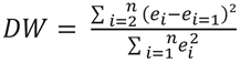 , where values near 2 indicate no autocorrelation and values well below 2 indicate positive autocorrelation. For a single-specimen degradation record with monotonically increasing cumulative UV, positive residual autocorrelation is expected: each observation inherits the specimen’s current microstructural damage state from the previous one. The Ljung-Box Q(1) test was applied alongside DW to confirm the direction and strength of the serial dependence.
, where values near 2 indicate no autocorrelation and values well below 2 indicate positive autocorrelation. For a single-specimen degradation record with monotonically increasing cumulative UV, positive residual autocorrelation is expected: each observation inherits the specimen’s current microstructural damage state from the previous one. The Ljung-Box Q(1) test was applied alongside DW to confirm the direction and strength of the serial dependence.Where both violations were present, Newey-West HAC standard errors were applied to all regression models. HAC standard errors use a Bartlett kernel-weighted sandwich estimator to produce valid inference under simultaneous heteroscedasticity and autocorrelation (Greene, 2020). Bandwidth was set by . OLS and WLS coefficient estimates are unbiased under autocorrelation and remain unchanged; only the standard errors and derived test statistics are corrected. Figure 1 shows OLS residual diagnostics; Figure 2 shows the WLS residual comparison.
3.5. Second-Order Polynomial Regression Model
A second-order polynomial regression model was developed to capture quadratic and interaction effects among the stressors, following the polynomial modeling framework in Chen et al. (2025). Wind speed was excluded from the polynomial model: its Pearson correlation was negligible (r = +0.065) and its OLS coefficient was non-significant even before HAC correction (t = 1.17, p = 0.243). The retained stressors were UVcum, temperature, and relative humidity:
Parameters were estimated by OLS. All standard errors are Newey-West HAC-corrected. Non-significant main effects were retained where their interaction or quadratic terms were significant, following the effect-heredity principle. Specifically, the non-significant linear Temperature and RH main effects were retained because their quadratic and interaction terms (T2, T × RH, RH2, UV × RH) are statistically significant after HAC correction. Term significance was assessed at α = 0.05 using HAC-corrected t-statistics. Figure 3 shows fitted-value contour plots for the two interactions that remained significant after HAC correction.
3.6. Reliability Analysis: Weibull and Lognormal Distributions
Two distributions were fitted to the tensile strength data by maximum likelihood estimation. The two-parameter Weibull probability density function is (Nelson, 2021):
where β > 0 is the shape parameter, η > 0 is the scale parameter, and x denotes tensile strength in MPa. The corresponding reliability function is . The lognormal probability density function is (Nelson, 2021):
where x is tensile strength in MPa, and μ and σ are the log-scale location and scale parameters. Model selection used (where is the maximized log-likelihood and k the number of parameters), , and the Kolmogorov-Smirnov statistic. The standard KS critical value for known parameters at n = 511 and α = 0.05 is 1.358/√511 ≈ 0.060. Because parameters were estimated from the data, the Li (2020) modified threshold of 0.895/√511 ≈ 0.040 is the relevant benchmark, and KS is used as a relative diagnostic rather than a standalone pass/fail test. Figure 4 shows both probability plots.
The B10 threshold used here is the 10th percentile of the fitted tensile strength distribution, meaning the strength value below which 10% of the statistical population falls under the model. This is a strength-based reliability criterion, distinct from the conventional time-to-failure B10 life. The cumulative UV dose at which the population-mean predicted tensile strength reaches the B10 threshold is obtained by inverting the OLS regression equation (Equation 1) with temperature, relative humidity, and wind speed held at their dataset means (14.05 °C, 78.92%, and 2.15 m/s, respectively). Conversion to an estimated service life uses a reference UV accumulation rate of 15 MJ/m2/year for mid-latitude temperate US conditions (Kempe et al., 2021). Sites with different irradiance levels should substitute local values.
3.7. Cost-Benefit Analysis
A discounted cost-benefit analysis compared standard PPE and premium fluoropolymer backsheet strategies over a 25-year module design life. Total cost follows the TC = FC + VC framework. Initial costs are $25/module (standard PPE) and $55/module (premium fluoropolymer), from PV bill-of-materials data (Ramasamy et al., 2021; IRENA, 2023). The total field replacement cost of $92/module, covering material, de-mounting, re-lamination, reinstallation, and downtime, draws on O&M benchmarks from Lawrence Berkeley National Laboratory (Wiser et al., 2020). A 6% annual discount rate was applied (IRENA, 2023), with the standard backsheet replacement cycle set at 15.4 years from the Weibull B10 result, giving NPV = $92/(1.06)15.4 = $37.55 per module. Break-even was solved as: the premium strategy is favored when undiscounted replacement cost exceeds $30 × (1.06)15.4 ≈ $74/module.
4. Results
4.1. Pearson Correlation Analysis
Cumulative UV irradiance correlated with tensile strength at r = −0.960 (R2 = 0.921, p < 0.001), accounting for 92.1% of total variance on its own. Temperature (r = −0.040), relative humidity (r = +0.143), and wind speed (r = +0.065) each showed negligible to weak individual associations. Results are in Table 2.
UV absorption in PET drives Norrish-type chain scission at carbonyl ester bonds, producing chromophoric oxidation products that steadily weaken the laminate (Lin et al., 2016; Zhang et al., 2022). The positive humidity correlation (r = +0.143) is weak in isolation but does not rule out an interactive contribution: absorbed moisture can delay brittle crack propagation at intermediate UV doses, while accelerating hydrolytic chain scission at higher doses (Kempe et al., 2021). Field studies in harsh multi-stressor climates confirm that interaction effects can account for substantial additional degradation beyond UV alone (Hameed et al., 2024).
4.2. OLS Multiple Linear Regression and ANOVA
The OLS model explained 92.5% of total tensile strength variance (R2 = 0.9249, RMSE = 4.715 MPa; F(4, 506) = 1557.90, p < 0.001). The fitted equation is:
The UV coefficient (β1 = −0.2245 MPa per MJ/m2) projects to a total tensile strength reduction of approximately 60.8 MPa across the observed UV range, or 25.1% of the initial value of 241.93 MPa. This sits close to the 26.7% reduction Lin et al. (2016) measured experimentally under comparable outdoor conditions, providing external validation. The ANOVA decomposition is in Table 3; coefficient estimates are in Table 4 and Table 5.
4.3. Autocorrelation Test Results and HAC Correction
The Durbin-Watson statistic for the OLS residuals was 0.038, far below the lower critical bound of approximately 1.82 for n = 511, k = 4 at α = 0.05. The lag-1 residual autocorrelation was ρ1 = 0.981, and the Ljung-Box Q(1) test confirmed the result decisively (Q = 494.6, p < 0.001). After fitting the polynomial model, which absorbs the primary systematic UV trend, the DW statistic improved only to 0.231 and the lag-1 autocorrelation remained at 0.884. Autocorrelation persisted because each observation carries forward the specimen’s accumulated microstructural damage state from the preceding one, a form of temporal dependence that the regression model itself cannot remove.
The practical consequence is that the conventional OLS standard errors in Table 4 are too small. After Newey-West HAC correction (Table 5), the UVcum standard error rises from 0.00402 to 0.00867 and its t-statistic changes from −55.85 to −25.89. Despite this, UVcum remains highly significant (p < 0.001), and relative humidity retains significance (t = 2.84, p = 0.005). Temperature and wind speed were non-significant before and after correction. The primary degradation finding is unaltered: UV irradiance drives tensile strength loss, and the rate is 0.2245 MPa per MJ/m2.
The WLS model with inverse-variance weights wi = (UVcum,i + 1)−0.6432 achieved weighted R2 = 0.9535 (F(4, 506) = 2592.71, p < 0.001). The fitted WLS equation is:
The unweighted RMSE under WLS is 4.870 MPa, marginally above the OLS value of 4.715 MPa, which is expected: WLS minimizes weighted residual variance and trades a small increase in raw prediction error for substantially improved inference in the high-variance region. The UV coefficient is stable at −0.2245 (OLS) versus −0.2111 (WLS), confirming the rate of UV-driven degradation is consistent across both estimators. Figure 2 shows the residual spread before and after WLS correction.
4.4. Second-Order Polynomial Regression Results
The polynomial model achieved R2 = 0.9686 (adjusted R2 = 0.9681, RMSE = 3.033 MPa; F(9, 501) = 1718.28, p < 0.001), a 35.4% reduction in prediction error relative to OLS. Table 6 presents all ten model terms with HAC-corrected standard errors. After HAC correction, six terms are significant at α = 0.05: UV, UV2, T2, RH2, UV × RH, and T × RH. The UV × Temperature interaction, which appeared significant under OLS standard errors (t = −3.80, p < 0.001), does not survive HAC correction (t = −1.56, p = 0.119), a direct illustration of how serial autocorrelation inflates inferential confidence. Figure 3 shows contour plots for the two HAC-significant interactions.
4.5. Reliability Analysis: Weibull vs. Lognormal
Maximum likelihood fitting returned Weibull parameters of β = 15.87 and η = 222.56 MPa, and lognormal parameters of μ = 5.368 and σ = 0.083. A shape parameter of 15.87 places the failure mode firmly in the wear-out regime, consistent with the accelerating UV2 effect confirmed in the polynomial model. The Weibull distribution outperformed the lognormal on all three selection criteria: AIC (4290.85 vs. 4394.23; ΔAIC = 103.38), BIC (4299.32 vs. 4402.71), and KS statistic (0.1453 vs. 0.2207). Model selection results are in Table 7 and probability plots in Figure 4.
Both KS statistics exceed the standard threshold of 0.060 and the Li (2020) modified critical value of approximately 0.040 for estimated parameters, meaning neither distribution achieves a perfect absolute fit. The 511 observations form a single serially autocorrelated time series (DW = 0.038; ρ1 = 0.981); distribution fitting by maximum likelihood assumes independence, so the reported AIC, BIC, and KS values should be interpreted as comparative indicators rather than exact information-theoretic quantities. The relative superiority of Weibull is nevertheless unambiguous: a ΔAIC of 103.38 over the lognormal is decisive under any reasonable adjustment, and the Weibull is the correct distributional choice for this material and dataset.
The B10 threshold, the 10th percentile of the fitted Weibull distribution, is 193.14 MPa, corresponding to a 20.2% reduction from the initial tensile strength of 241.93 MPa. Inverting the OLS regression equation (Equation 5) with T, RH, and WS held at their dataset means, this B10 strength level is reached at approximately 231.3 MJ/m2 of cumulative UV, or roughly 15.4 years at a reference UV accumulation rate of 15 MJ/m2/year (Kempe et al., 2021). Planners may use this as a maintenance planning threshold: the population-mean predicted tensile strength of the PPE backsheet reaches the B10 level at approximately year 15 under temperate mid-latitude conditions.
4.6. Cost-Benefit Analysis
Setting the standard PPE replacement cycle at 15.4 years from the Weibull B10 result, the NPV of the $92 field replacement cost discounted at 6% is $37.55 per module, giving the standard strategy a total NPV of $62.55. The premium fluoropolymer strategy, with no replacement event within the 25-year design life, has a total NPV of $55.00. The premium strategy carries a $7.55 per module NPV advantage. Table 8 provides the complete breakdown.
The break-even threshold is an undiscounted field replacement cost of approximately $74 per module. Since the current estimate of $92 sits $18 above that threshold, the premium strategy is financially justified across a meaningful range of cost uncertainty. At 50,000 to 500,000 modules per utility installation, the per-module advantage aggregates to between $375,000 and $3.75 million in avoided lifecycle costs per project.
5. Discussion
The most important thing this dataset communicates is also the simplest: UV radiation is what breaks down this backsheet. At the bivariate level, cumulative UV explains 92.1% of tensile strength variance before any other stressor enters the picture. That figure comes from a single Pearson correlation, not from model complexity. UV absorption in PET drives Norrish Type I and Type II reactions at carbonyl ester bonds, releasing chain scission byproducts that progressively reduce the laminate’s tensile capacity. The WPET outer layer bears the highest UV load and is the first to embrittle, as the channel cracking data in Lin et al. (2016) showed directly. At high enough accumulated doses, this embrittlement works inward through the PET core.
The autocorrelation finding carries real inferential weight. A DW statistic of 0.038 and a lag-1 residual autocorrelation of 0.981 reflect the physical reality of the measurement design: a single specimen measured at 511 points along its degradation trajectory. Each observation inherits the specimen’s current damage state from the one before it. OLS standard errors in this setting are too small, and the conventional t-statistics are inflated. After Newey-West HAC correction, UVcum remains highly significant at t = −25.89, so the primary finding about degradation rate is unchanged. What does change is the UV × Temperature interaction: it appeared significant under OLS (p < 0.001) and lost significance after HAC correction (p = 0.119). Temperature effects in this dataset appear to operate through the quadratic T2 term and through co-action with humidity, rather than through a direct multiplicative interaction with UV dose. That is a substantive finding about the mechanism, not a technical footnote.
The two polynomial interactions that survived HAC correction are physically interpretable. The positive UV × RH coefficient (β = +0.00145, p < 0.001) suggests that at the UV doses observed here, higher humidity is associated with marginally better tensile strength retention, plausibly because absorbed moisture plasticizes the PET surface layer and delays brittle crack propagation. Whether this reverses at higher UV levels, where hydrolytic chain scission would dominate, cannot be determined from this dataset. The positive T × RH coefficient (β = +0.01172, p < 0.001) suggests a partial compensating effect when both temperature and humidity are elevated simultaneously, possibly through moisture-driven suppression of thermally induced crystallization in amorphous PET domains.
The Weibull result is unambiguous. A ΔAIC of 103.38 over the lognormal is decisive by any accepted standard, and the shape parameter of 15.87 describes a physically coherent wear-out pattern. Neither distribution achieves a perfect absolute KS fit, but for a single-specimen degradation record with heterogeneous microcrack distributions, this is expected rather than surprising. The B10 threshold of 193.14 MPa at roughly 15.4 years translates directly into a maintenance planning horizon: the population-mean predicted tensile strength reaches this level at approximately 231.3 MJ/m2 of cumulative UV under temperate mid-latitude conditions.
Economics reinforce this timeline. A $7.55 per module NPV advantage for premium fluoropolymer looks modest in isolation, but it holds across a wide range of cost because the break-even threshold is $74 per module and field labor costs alone typically exceed that (Wiser et al., 2020). The remaining analytical limitations worth flagging are the reliance on a single UV accumulation rate of 15 MJ/m2/year; the use of a single-specimen dataset, which means material-to-material variability cannot be separated from temporal autocorrelation. Future work should build stochastic, location-specific irradiance projections into the analysis to convert the B10 result into a climate-adjusted service life distribution rather than a single point estimate and should extend the dataset to multiple specimens to address both limitations simultaneously.
6. Conclusion
Using 511 sequential field measurements from a multilayer PPE PV backsheet spanning 271.6 MJ/m2 of cumulative UV exposure, this paper developed and validated a six-stage statistical framework for tensile strength degradation modeling. The key findings fall into three groups.
On the degradation physics: cumulative UV irradiance is the decisive driver, explaining 92.1% of tensile strength variance on its own (r = −0.960) and remaining the dominant predictor at t = −25.89 after full statistical correction. The OLS model predicted a 25.1% total tensile strength reduction, closely matching the 26.7% measured by Lin et al. (2016) under comparable conditions. The second-order polynomial model reduced predictive error by 35.4% (RMSE from 4.715 to 3.033 MPa), and six nonlinear and interaction terms survived HAC correction: UV, UV2, T2, RH2, UV × RH, and T × RH.
On statistical validity: significant heteroscedasticity (BP LM = 192.93, p < 0.001) and very strong serial autocorrelation (DW = 0.038, ρ1 = 0.981) were both detected and corrected. WLS addressed heteroscedasticity and improved weighted R2 to 0.9535. Newey-West HAC standard errors corrected all inferential tests. Coefficient estimates are unbiased and unchanged; the corrections affect only standard errors and test statistics derived. The UV × Temperature interaction, significant under OLS, lost significance after HAC correction and should not be over-interpreted.
On reliability and cost: Weibull fitting was decisively superior to lognormal (ΔAIC = 103.38), returning β = 15.87 and a B10 tensile strength threshold of 193.14 MPa at approximately 15.4 years. Cost-benefit analysis demonstrated a $7.55 per module NPV advantage for premium fluoropolymer backsheets, with the premium strategy financially justified whenever undiscounted field replacement costs exceed roughly $74 per module.
The framework developed here, covering Pearson screening, OLS/WLS regression with Breusch-Pagan and Durbin-Watson diagnostics, Newey-West HAC correction, polynomial modeling, and Weibull reliability analysis, is directly transferable to other backsheet materials and degradation modes. Future work should extend the approach to multi-specimen datasets to separate material variability from temporal autocorrelation and should incorporate site-specific stochastic UV projections to generate climate-adjusted service life distributions.
Author’s Note
This study was undertaken as a part of doctoral dissertation research conducted at the Morgan State University in the Department of Industrial and Systems Engineering under the supervision and guidance of the dissertation committee, chaired by Dr. Tridip K. Bardhan.
References
- Al Mahdi, H.; Leahy, P. G.; Alghoul, M.; Morrison, A. P. A Review of Photovoltaic Failure and Degradation Mechanisms. Solar 2023, 4(1), 43–82. [Google Scholar] [CrossRef]
- Boon-on, P.; Lien, S.; Chang, T.; Shi, J.; Lee, M. Band gap engineered ternary semiconductor PbxCd1−xS: Nanoparticle-sensitized solar cells with an efficiency of 8.5% under 1% sun—A combined theoretical and experimental study. Progress in Photovoltaics: Research and Applications 2020, 28(4), 328–341. [Google Scholar] [CrossRef]
- Chen, H.-Y.; Chen, C. A Study of the Response Surface Methodology Model with Regression Analysis in Three Fields of Engineering. Applied System Innovation 2025, 8(4), 99–99. [Google Scholar] [CrossRef]
- Damo, U. M.; Ozoegwu, C. G.; Ogbonnaya, C.; Maduabuchi, C. Effects of light, heat and relative humidity on the accelerated testing of photovoltaic degradation using Arrhenius model. Solar Energy 2023, 250, 335–346. [Google Scholar] [CrossRef]
- Gaddam, S. K.; Pothu, R.; Boddula, R. Advanced polymer encapsulates for photovoltaic devices − A Review. Journal of Materiomics 2021, 7(5), 920–928. [Google Scholar] [CrossRef]
- Hameed, M. A.; Kaaya, I.; Al-Jbori, M.; Matti, Q.; Scheer, R.; Gottschalg, R. Analysis and prediction of the performance and reliability of PV modules installed in harsh climates: Case study Iraq. Renewable Energy 2024, 228, 120577–120577. [Google Scholar] [CrossRef]
- IRENA. Renewable Power Generation Costs in 2022; Www.irena.org., 2023; Available online: https://www.irena.org/Publications/2023/Aug/Renewable-Power-Generation-Costs-in-2022.
- Kempe, M. D.; Lyu, Y.; Kim, J. H.; Felder, T.; Gu, X. Fragmentation of photovoltaic backsheets after accelerated weathering exposure. Solar Energy Materials and Solar Cells 2021, 226, 111044. [Google Scholar] [CrossRef]
- Kumar, N. K. Autocorrelation and Heteroscedasticity in Regression Analysis. Journal of Business and Social Sciences 2023, 5(1), 9–20. [Google Scholar] [CrossRef]
- Li, J. EDF goodness-of-fit tests based on centre-outward ordering. Journal of Nonparametric Statistics 2020, 30(4), 973–989. [Google Scholar] [CrossRef]
- Li, Y.; Peng, S.; Li, Y.; Jiang, W. A review of condition-based maintenance: Its prognostic and operational aspects. Frontiers of Engineering Management 2020, 7(3), 323–334. [Google Scholar] [CrossRef]
- Lin, C.-C.; Lyu, Y.; Yu, L.-C.; Gu, X. Correlation between mechanical and chemical degradation after outdoor and accelerated laboratory aging for multilayer photovoltaic backsheets. Proceedings of SPIE, the International Society for Optical Engineering/Proceedings of SPIE; 2016. [Google Scholar] [CrossRef]
- Lv, Y.; Fairbrother, A.; Gong, M.; Kim, J. H.; Gu, X.; Kempe, M.; Julien, S.; Wan, K.; Napoli, S.; Hauser, A. W.; O’Brien, G.; Wang, Y.; French, R. H.; Bruckman, L. S.; Ji, L.; Boyce, K. P. Impact of environmental variables on the degradation of photovoltaic components and perspectives for the reliability assessment methodology. Solar Energy 2020, 199, 425–436. [Google Scholar] [CrossRef]
- Markert, J.; Ensslen, F.; Rist, T.; Beinert, A. J.; Job, E.; Hädrich, I.; Philipp, D. Mechanical Stability of PV Modules. PV-Symposium Proceedings 2024, 1. [Google Scholar] [CrossRef]
- Mitterhofer, S.; Kempe, M.; Gu, X. Evaluation of Surface Crack Formation in Photovoltaic Backsheets Using Fragmentation and Finite Element Simulations. IEEE Journal of Photovoltaics 2024, 14(2), 311–318. [Google Scholar] [CrossRef]
- Nelson, W. B. Statistical Methods for Reliability Data, Second Edition. Technometrics 2021, 63(3), 437–440. [Google Scholar] [CrossRef]
- Ramasamy, V.; Feldman, D.; Desai, J.; Margolis, R. U.S. Solar Photovoltaic System and Energy Storage Cost Benchmark: Q1 2021; Technical Report; 2021. [Google Scholar] [CrossRef]
- Shama, M. S.; Alharthi, A. S.; Almulhim, F. A.; Gemeay, A. M.; Meraou, M. A.; Mustafa, M. S.; Hussam, E.; Aljohani, H. M. Modified generalized Weibull distribution: theory and applications. Scientific Reports 2023, 13(1). [Google Scholar] [CrossRef] [PubMed]
- Smith, S.; Mitterhofer, S.; Moffitt, S. L.; Jhang, S.-S.; Watson, S. S.; Sung, L.-P.; Gu, X. Long-term durability of transparent backsheets for bifacial photovoltaics: An in-depth degradation analysis. Solar Energy Materials & Solar Cells/Solar Energy Materials and Solar Cells 2023, 256, 112309–112309. [Google Scholar] [CrossRef]
- Tan, V.; Dias, P. R.; Chang, N.; Deng, R. Estimating the Lifetime of Solar Photovoltaic Modules in Australia. Sustainability 2022, 14(9), 5336. [Google Scholar] [CrossRef]
- Wiser, R.; Bolinger, M.; Seel, J. Benchmarking Utility-Scale PV Operational Expenses and Project Lifetimes: Results from a Survey of U.S. Solar Industry Professionals. 2020. Available online: https://eta-publications.lbl.gov/sites/default/files/solar_life_and_opex_report.pdf.
- Zhang, J.-W.; Feng, K.; Diaham, S.; Liao, Q.-Q.; Zhou, X.; Putson, C. Lifetime Evaluation of Photovoltaic Polymeric Backsheets under Ultraviolet Radiation: From Chemical Properties to Mechanical Modeling. ACS Omega 2022, 7(49), 45609–45616. [Google Scholar] [CrossRef] [PubMed]
Figure 1.
OLS residual diagnostics. Panel (A): residual spread widens markedly with increasing UV dose, confirming heteroscedasticity (BP LM = 192.93, p < 0.001) and autocorrelation (DW = 0.038). Panel (B): normal Q-Q plot of OLS residuals.
Figure 1.
OLS residual diagnostics. Panel (A): residual spread widens markedly with increasing UV dose, confirming heteroscedasticity (BP LM = 192.93, p < 0.001) and autocorrelation (DW = 0.038). Panel (B): normal Q-Q plot of OLS residuals.
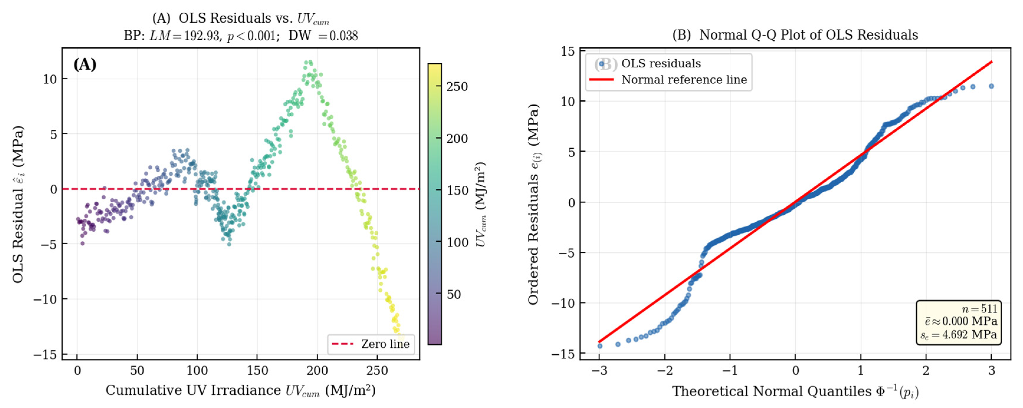
Figure 2.
OLS vs. WLS residual comparison. Panel (A): growing spread under OLS. Panel (B): more uniform spread after WLS correction (wi = (UVcum,i + 1)−0.6432). Weighted R2 improves from 0.9249 to 0.9535.
Figure 2.
OLS vs. WLS residual comparison. Panel (A): growing spread under OLS. Panel (B): more uniform spread after WLS correction (wi = (UVcum,i + 1)−0.6432). Weighted R2 improves from 0.9249 to 0.9535.
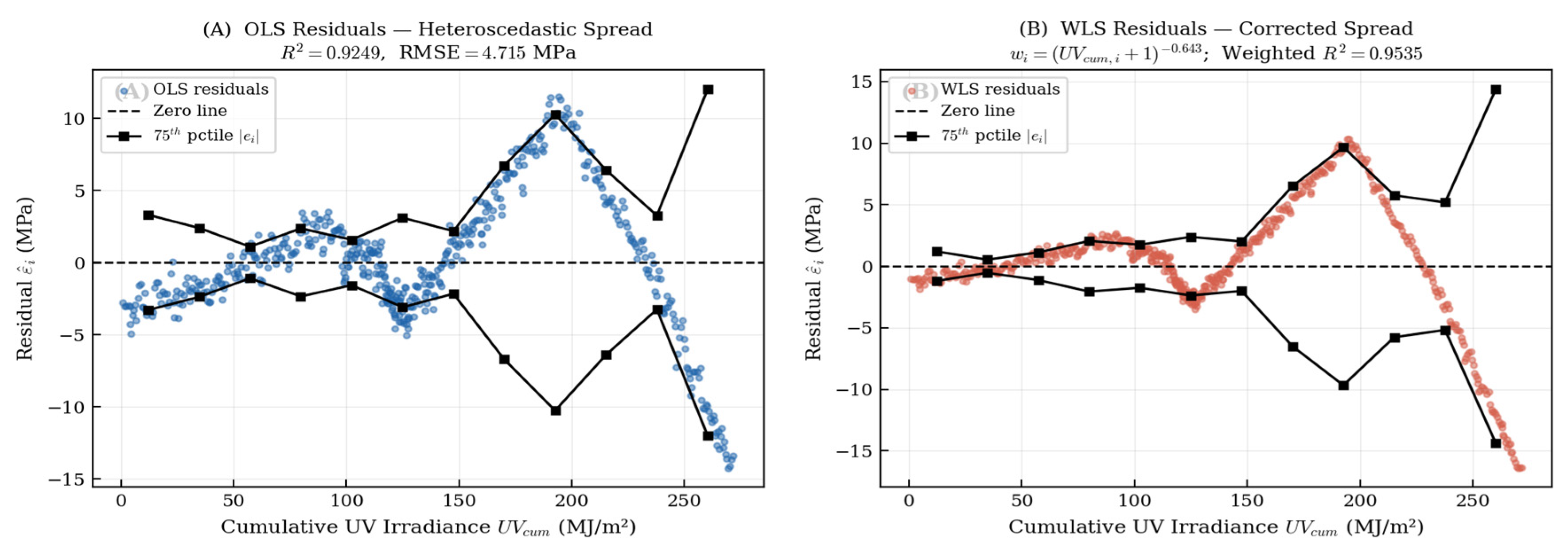
Figure 3.
Second-order polynomial regression fitted-value contour plots. Panel (A): UVcum × RH interaction (T held at mean = 14.1 °C; RH held at mean = 78.9% on y-axis). Panel (B): Temperature × RH interaction (UVcum held at mean = 133.7 MJ/m2). Both interactions remain significant after Newey-West HAC correction. Green = higher predicted tensile strength (MPa); red = greater predicted degradation. R2 = 0.9686, RMSE = 3.033 MPa.
Figure 3.
Second-order polynomial regression fitted-value contour plots. Panel (A): UVcum × RH interaction (T held at mean = 14.1 °C; RH held at mean = 78.9% on y-axis). Panel (B): Temperature × RH interaction (UVcum held at mean = 133.7 MJ/m2). Both interactions remain significant after Newey-West HAC correction. Green = higher predicted tensile strength (MPa); red = greater predicted degradation. R2 = 0.9686, RMSE = 3.033 MPa.
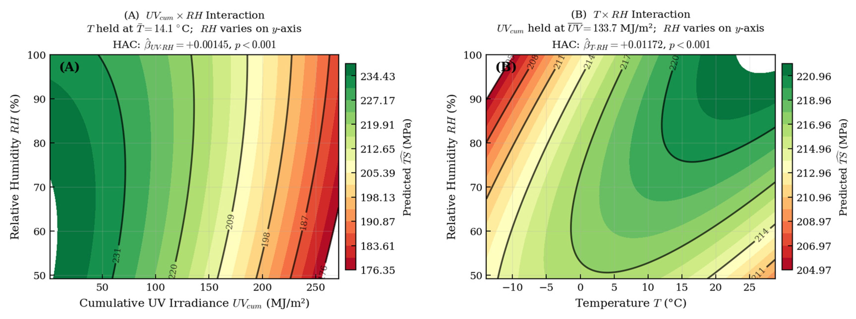
Figure 4.
Weibull and lognormal probability plots (median-rank positions). Panel (A): Weibull fit (β = 15.87, η = 222.56 MPa, KS = 0.1453). Panel (B): Lognormal fit (μ = 5.368, σ = 0.083, KS = 0.2207). Weibull is decisively superior (ΔAIC = 103.38). Both KS statistics exceed the Li (2020) modified critical value; see Table 7 footnote.
Figure 4.
Weibull and lognormal probability plots (median-rank positions). Panel (A): Weibull fit (β = 15.87, η = 222.56 MPa, KS = 0.1453). Panel (B): Lognormal fit (μ = 5.368, σ = 0.083, KS = 0.2207). Weibull is decisively superior (ΔAIC = 103.38). Both KS statistics exceed the Li (2020) modified critical value; see Table 7 footnote.
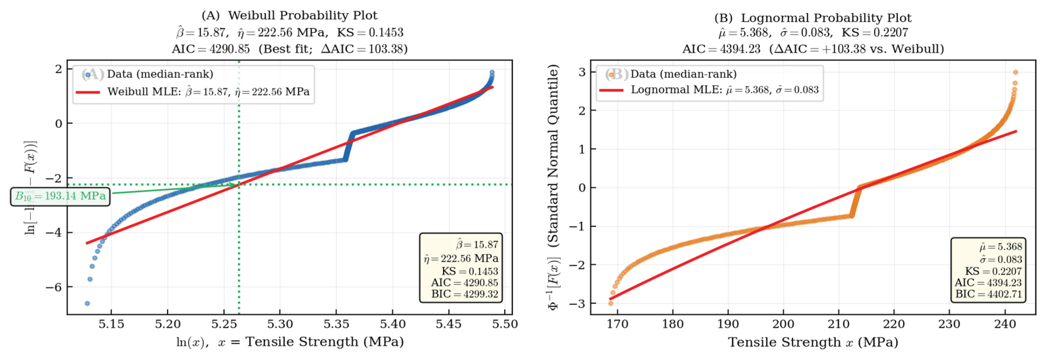

Table 1.
Descriptive Statistics for the 511-Observation Field Dataset.
| Variable | n | Min | Max | Mean | Std Dev | Median |
|---|---|---|---|---|---|---|
| Temperature (°C) | 511 | −13.84 | 28.74 | 14.05 | 10.46 | 17.87 |
| Relative Humidity (%) | 511 | 49.18 | 100.00 | 78.92 | 10.03 | 79.29 |
| Wind Speed (m/s) | 511 | 0.76 | 7.28 | 2.15 | 0.88 | 1.98 |
| Cumul. UV (MJ/m2) | 511 | 0.84 | 271.6 | 133.7 | 72.9 | 126.7 |
| Tensile Strength (MPa) | 511 | 168.76 | 241.93 | 215.15 | 17.14 | 213.73 |
Table 2.
Pearson Correlation Coefficients Between Environmental Stressors and Tensile Strength (n = 511).
Table 2.
Pearson Correlation Coefficients Between Environmental Stressors and Tensile Strength (n = 511).
| Environmental Stressor | r (Pearson) | R2 | Interpretation |
|---|---|---|---|
| Cumulative UV (MJ/m2) | −0.960 | 0.921 | Dominant driver |
| Temperature (°C) | −0.040 | 0.002 | Negligible |
| Relative Humidity (%) | +0.143 | 0.020 | Weak positive |
| Wind Speed (m/s) | +0.065 | 0.004 | Negligible |
Table 3.
ANOVA Table for OLS Multiple Linear Regression Model.
| Source | SS | df | MS | F | p-value |
|---|---|---|---|---|---|
| Regression | 138,537.7 | 4 | 34,634.4 | 1557.90 | < 0.001 |
| Residual | 11,250.3 | 506 | 22.23 | -- | -- |
| Total | 149,788.0 | 510 | -- | -- | -- |
Table 4.
OLS Coefficient Estimates with Standard OLS Standard Errors. (R2 = 0.9249, RMSE = 4.715 MPa).
Table 4.
OLS Coefficient Estimates with Standard OLS Standard Errors. (R2 = 0.9249, RMSE = 4.715 MPa).
| Term | Coefficient | OLS Std Error | t | p-value |
|---|---|---|---|---|
| Intercept | 237.016 | 3.142 | 75.43 | < 0.001 |
| UVₜᵤₘ (MJ/m2) | −0.2245 | 0.00402 | −55.85 | < 0.001 |
| Temperature (°C) | 0.0034 | 0.0272 | 0.13 | 0.902 |
| Relative Humidity (%) | 0.0927 | 0.0284 | 3.26 | 0.001 |
| Wind Speed (m/s) | 0.3644 | 0.312 | 1.17 | 0.243 |
Table 5.
OLS Coefficient Estimates with Newey-West HAC Standard Errors. (DW = 0.038, ρ1 = 0.981; bandwidth h = 5; n = 511).
Table 5.
OLS Coefficient Estimates with Newey-West HAC Standard Errors. (DW = 0.038, ρ1 = 0.981; bandwidth h = 5; n = 511).
| Term | Coefficient | HAC Std Error | t (HAC) | p (HAC) |
|---|---|---|---|---|
| Intercept | 237.016 | 2.589 | 91.56 | < 0.001 |
| UVₜᵤₘ (MJ/m2) | −0.2245 | 0.00867 | −25.89 | < 0.001 |
| Temperature (°C) | 0.0034 | 0.03182 | 0.11 | 0.914 |
| Relative Humidity (%) | 0.0927 | 0.03262 | 2.84 | 0.005 |
| Wind Speed (m/s) | 0.3644 | 0.24031 | 1.52 | 0.130 |
Coefficient estimates are identical to OLS; HAC correction changes only standard errors and derived statistics. Bold = HAC-significant (p < 0.05). UVₜᵤₘ t-statistic falls from −55.85 (OLS) to −25.89 (HAC) but remains highly significant. RH retains significance (p = 0.005).
Table 6.
Polynomial Regression Coefficient Estimates with Newey-West HAC Standard Errors (R2 = 0.9686, RMSE = 3.033 MPa; F(9, 501) = 1718.28; DW = 0.231, ρ1 = 0.884).
Table 6.
Polynomial Regression Coefficient Estimates with Newey-West HAC Standard Errors (R2 = 0.9686, RMSE = 3.033 MPa; F(9, 501) = 1718.28; DW = 0.231, ρ1 = 0.884).
| Term | Coefficient | HAC Std Error | t (HAC) | p (HAC) | Sig. |
|---|---|---|---|---|---|
| Intercept | 234.064 | 7.210 | 32.39 | < 0.001 | *** |
| UV (MJ/m2) | −0.1434 | 0.04875 | −2.94 | 0.003 | ** |
| Temperature (°C) | −0.2865 | 0.16904 | −1.70 | 0.091 | ns† |
| Rel. Humidity (%) | +0.2292 | 0.17660 | 1.30 | 0.195 | ns† |
| UV2 | −0.000580 | 0.000113 | −5.11 | < 0.001 | *** |
| Temperature2 | −0.01178 | 0.002780 | −4.24 | < 0.001 | *** |
| RH2 | −0.003360 | 0.001140 | −2.95 | 0.003 | ** |
| UV × Temperature | −0.001590 | 0.001020 | −1.56 | 0.119 | ns‡ |
| UV × Rel. Humidity | +0.001450 | 0.000440 | 3.34 | < 0.001 | *** |
| Temperature × RH | +0.01172 | 0.001730 | 6.80 | < 0.001 | *** |
*** p < 0.001; ** p < 0.01; ns = not significant after HAC. † Linear T and RH main effects retained under effect-heredity principle (their quadratic and interaction terms are significant). ‡ UV × Temperature was significant under OLS SEs (t = −3.80, p < 0.001) but loses significance after Newey-West HAC correction (p = 0.119). Coefficient estimates are unbiased; only SEs and derived statistics differ from OLS.
Table 7.
Reliability Distribution Model Comparison (n = 511).
| Distribution | Parameters | AIC | BIC | KS Stat. | Verdict |
|---|---|---|---|---|---|
| Weibull | β = 15.87, η = 222.56 MPa | 4290.85 | 4299.32 | 0.1453 | Best fit |
| Lognormal | μ = 5.368, σ = 0.083 | 4394.23 | 4402.71 | 0.2207 |
KS standard critical value (known parameters, n = 511, α = 0.05): ≈0.060. Modified critical value for estimated parameters (Li, 2020): ≈0.040. Neither distribution achieves a perfect KS-based fit; model selection rests on AIC/BIC (ΔAIC = 103.38, decisive). AIC/BIC values are indicative given serially dependent observations; the Weibull advantage is robust under any reasonable autocorrelation adjustment.
Table 8.
Cost-Benefit Analysis: NPV of Total Costs per Module over 25-Year Design Life.
| Cost Component | Standard PPE | Premium Fluoropolymer |
|---|---|---|
| Initial backsheet cost ($/module) | $25.00 | $55.00 |
| Replacement cycle (years) | ~15.4 | None (25-yr life) |
| Field replacement cost (undiscounted) | $92.00 | $0.00 |
| Replacement cost NPV @ 6%, 15.4 yrs | $37.55 | $0.00 |
| Total NPV of costs ($/module) | $62.55 | $55.00 |
Initial material costs: Fu et al. (2021) and IRENA (2023). Field replacement cost ($92/module): Wiser et al. (2020); includes backsheet material, de-mounting, relamination, reinstallation, and downtime. Discount rate 6% p.a.: IRENA (2023). Replacement cycle from Weibull B10 result. Break-even undiscounted replacement cost ≈ $74/module.
Disclaimer/Publisher’s Note: The statements, opinions and data contained in all publications are solely those of the individual author(s) and contributor(s) and not of MDPI and/or the editor(s). MDPI and/or the editor(s) disclaim responsibility for any injury to people or property resulting from any ideas, methods, instructions or products referred to in the content. |
© 2026 by the authors. Licensee MDPI, Basel, Switzerland. This article is an open access article distributed under the terms and conditions of the Creative Commons Attribution (CC BY) license (http://creativecommons.org/licenses/by/4.0/).
Copyright: This open access article is published under a Creative Commons CC BY 4.0 license, which permit the free download, distribution, and reuse, provided that the author and preprint are cited in any reuse.


