

Submitted:
01 July 2026
Posted:
02 July 2026
You are already at the latest version
Abstract
Quarry waste piles are heterogeneous engineered embankments that are susceptible to slope instability, yet early detection of pre-failure surface changes remains challenging due to complex surface conditions and measurement uncertainty. This study presents an integrated remote sensing–based framework for monitoring quarry waste pile instability by combining multi-temporal change detection with scale-dependent surface roughness analysis. Multi-epoch UAV-mounted LiDAR and photogrammetric point clouds were acquired before and after documented failure events at multiple active quarry sites. A standardized workflow was implemented, including precision alignment using a Recursive Iterative Closest Point (R-ICP) registration strategy, vegetation filtering with a multiscale CANUPO classifier, and uncertainty quantification through a Level of Detection (LoD) analysis. The resulting LoD thresholds were 10–15 cm for LiDAR-to-LiDAR comparisons and 34–36 cm for mixed-sensor datasets. Multi-scale roughness analysis revealed that zones which later experienced instability exhibited consistently higher and more heterogeneous roughness than adjacent stable areas within a well-defined linear scale range. A roughness-based A/D indicator enabled objective delineation of hazardous zones prior to failure. Post-failure monitoring showed surface smoothing following major displacement, followed by renewed roughness increases associated with secondary movements. These results demonstrate that scale-dependent roughness provides complementary information to displacement-based change detection and supports proactive geohazard monitoring of quarry waste piles.
Keywords:
remote sensing
; geohazards
; landslides
; heterogeneous stockpiles
; failure precursors
; change detection analysis
1. Introduction
Urban densification around the world has led to large increase in generation of waste granular material from excavation debris and industrial mineral extraction. Quarries and small open pits near urban centers offer cost-effective solutions for granular material storage with direct incomes for operators. The resulting stockpiles present characteristic geotechnical and operational features and inherent stability challenges arising primarily from the very heterogeneous sources of stockpile materials [1]. Punctual instrumentation (e.g. inclinometers, radars) offer limited value due to important spatial variability. Topographical monitoring emerged as a robust alternative to detect and monitor stockpile stability along highly heterogeneous grounds.
Advances in remote sensing technologies have enabled high-resolution, three-dimensional characterization of slope surfaces [2,3,4]. LiDAR (i.e. Light Detection and Ranging) and photogrammetry systems mounted on unmanned aerial vehicles (UAV) offer rapid and repeatable acquisition of dense point clouds, to represent surface geometry. By comparing multi-temporal point clouds using differencing techniques, such as cloud-to-cloud (C2C), cloud-to-mesh (C2M), or more advanced direct cloud-to-cloud methods like the Multiscale Model-to-Model Cloud Comparison (M3C2), researchers can quantify surface changes at millimeter to centimeter scales across successive survey epochs [5,6,7,8]. These approaches provide robust distance measurements and uncertainty estimation, making them particularly effective for irregular and heterogeneous slope surfaces typical of quarry waste piles. Change detection analysis enables detailed quantification of topographic evolution, such as volumetric changes, surface erosion, deposition, and displacement patterns over time [9,10].
Recently published application cases also highlighted the effectiveness of UAV-mounted photogrammetry or LiDAR data acquisition for accurate change detection in a mineral extraction contexts. These technological solutions reportedly achieve sub-decimeter precision for mapping surface changes even on complex or partially vegetated embankments, thereby supporting ongoing stability assessments and operational planning near urban areas [11,12,13]. Through time-series analysis, these methods facilitate the computation of volumes, identification of active movement zones, and improved understanding of slope behavior under varying environmental conditions.
Change detection analysis (CDA) quality is controlled by the different error components and quantifiable uncertainty arising from the tools and methods implemented. The corresponding level of detection (LOD) is dictated explicitly by measurement repeatability (i.e. tool calibration), measurement distortion from high incidence angle, and co-registration. Efficient CDA must account for inherent uncertainty and minimize their influence on results through targeted controls in data acquisition and post-processing analysis.
Most published case-studies on slope failure events emphasized post-failure change detection. These analyses typically quantify displaced material volumes, delineate main scarp geometries, assess runout distances, and evaluate depositional features through multi-temporal digital elevation model comparisons or orthophoto differencing [12,13,14,15]. Such post-event assessments provide useful information in understanding failure mechanisms, validating numerical models, and informing remediation efforts.
Few studies have systematically examined pre-failure topographical patterns and their potential role as precursors to slope instability. While emerging applications of time-series InSAR, repeated terrestrial LiDAR, and UAV-based monitoring have begun to capture subtle pre-failure deformations such as accelerating displacements or crack propagation in rock slopes and landslides [8,16,17], systematic investigations remain limited, particularly for heterogeneous engineered embankments like quarry waste piles.
To address this gap, the present study examines superficial topographic characteristics of pre-failure zones in heterogenous stockpiles to identify potential failure precursors. A multiscale topographic analysis, analogous to the concept of fractals applied to geomorphologies [18,19] is applied to derive characteristic trends for surface roughness and geometric variability. These measures are compared between unstable and stable zones to detect distinctive patterns linked to impending failure, which may arise from progressive internal deformation or material weakening.
This work presents a case application of the proposed multi-scale topographic analysis to a heterogeneous stockpile located at a quarry operation near the greater Montreal (Canada) area. CDA monitoring was conducted at the stockpile via UAV-mounted LiDAR and photogrammetry from 2022 to 2025. Details of the semi-automated CDA workflow with LOD computations are presented at length. Accurate dataset alignment is emphasized, with an improved semi-iterative registration strategy employed to distinguish true topographic evolution from alignment artifacts. Two landslides with volumes of 700 m³ and 253 m³ that occurred on the stockpile in 2023 are investigated through standard CDA. The multi-scale analysis is then applied on the pre-failure topographical models to showcase precursor identification. The approach is extrapolated to other parts of the stockpile exhibiting variable levels of deformation.
The present research offers an integrated monitoring framework combining slope CDA with pre-failure surface characterization using high-resolution remote sensing. By emphasizing scale-dependent topographic features, it advances understanding of failure processes in quarry waste piles and supports the development of early warning indicators for safer slope management in and near urban settings.
2. Experimental Settings
The monitoring program showcased in this work was conducted at a limestone quarry producing aggregate and construction materials. The nearly 70 years old stockpile consists of overburden, processing waste, blasted oversize, low grade ore and construction debris. The stockpile geometry is characterized by irregular slope angles of up to 40 m varying from 30 to 45 degrees. The stockpile was constructed by a push-dump sequence without benches or recess in the slope.
The quarry (illustrated in Figure 1) is located approximately 60 km north of Montréal (Canada). The stockpile is located at the South-Western edge of the active quarry. It is bordered by agricultural fields to the North, and urban developments West and South. Stockpile construction is characteristic of constrained footprints near urban and peri-urban settings which favors steep slopes.
A distinct landslide event occurred along the north-west slope during spring 2023 (Figure 2), followed by several smaller failures in the subsequent years. The pile is regularly exposed to freeze–thaw cycles and rapid snowmelt, which contribute to surface erosion and transient pore-pressure increases (see also a numerical back-analysis of the landslide event presented in [20]).
The investigated failure event followed a period of rapid snowmelt in spring of 2023. These conditions led to temporary saturation within the overburden layers, increased pore-water pressures in the loosely compacted granular mixtures and sudden drop in apparent cohesion of the material. The landslide was reported in late March 2023 after several days of alternating freeze and thaw conditions accompanied by heavy rainfall. Field observations indicated a translational slide involving the upper portion of the northwestern wall, with an estimated displacement of several meters’ downslope. The initial failure produced a nearly vertical headwall and a hummocky deposit composed of coarse limestone fragments and fine backfill at the toe. Continued seepage along the failure surface and the development of small secondary rills in the following weeks suggested that the upper layer remained partially unstable.
Figure 3 shows aerial photographs from spring 2025 illustrating the current condition of the affected slope. Two distinct failure zones are highlighted in the figure. Zone A, located on the North side, corresponds to the larger and more active portion of the landslide, where the displaced material accumulated at the toe. Zone B, situated slightly west of Zone A, is smaller and shallower but displays similar evidence of surface disturbance and tension cracking. The South face of the pile remains sparsely vegetated, and the presence of leaning trees near the crest indicates continuing deformation or delayed stabilization. To reduce further downslope movement, large blocks were positioned along the toe to act as counterweights, forming a continuous stabilizing barrier (visible in Figure 3).
Figure 4 illustrates topographical models of studied section of the pile. The models were surveyed before (Figure 4a) and after (Figure 4b) the 2023 landslide. The post failure model reveals the formation of a pronounced scarp along the upper slope and a bulging accumulation zone near the toe. The displaced material produced an irregular and roughened surface (Figure 4b) that contrasts sharply with the smoother pre-failure geometry (Figure 4a). These two datasets were used in subsequent sections as reference epochs for the detailed change detection and monitoring workflow.
The topographical model for the pre-failure conditions (Figure 4a) was captured with UAV-mounted photogrammetry. The post failure model was captured with UAV-mounted LiDAR DJI Zenmuse L1. The achieved point spacing was 0.30 and 0.11 m for the pre- and post-failure models respectively.
Change detection analysis was conducted on the models illustrated in Figure 4 to quantify the topographic variations that occurred between the October 2022 (pre-failure) and April 2023 (post-failure) surveys. The analysis was performed using Cloud to Cloud (C2C) distance measurements using the open-source software CloudCompare V2.14 [5]. Co-registration was performed through recursive ICP placement following the workflow outlined in [21].
Figure 5 shows the results of the C2C analysis, which provided a first overview of the magnitude and spatial distribution of the surface changes. The results revealed two main areas of material loss concentrated along the central and western portions of the slope, where absolute distances locally exceeded 2.96 m. Blue and green colors represent stable or low-change regions, whereas yellow to red tones indicate significant displacement associated with the 2023 failure.
Figure 6 highlights the failure envelopes of Zone A and Zone B, corresponding to the principal detachment and subsidence sectors of the pile. Zone A spans approximately 21–25 m, while Zone B covers an area of roughly 14–17 m, reflecting the portions of the pile most affected by deformation. The estimated volumes of the displaced material are approximately 700 m³ for Zone A and 253 m³ for Zone B.
In Zone A, Figure 6 illustrates a maximum absolute displacement of 2.84 m, measured along the section passing through the most deformed portion of the western scarp. The extracted cross-section reveals the vertical collapse geometry of the detached block, representing the upper segment of the failure surface. In Zone B, Figure 6b presents the cross-section where the maximum absolute C2C distance of 2.76 m was recorded. The profile shows that deformation was concentrated near the crest of the eastern scarp, with the failure propagating downward through the slope. The measured displacements in both zones delineate the deepest portions of the failure surfaces and provide an estimate of the approximate thickness of the displaced mass.
These near-concurrent spring events highlighted the vulnerability of the waste piles to seasonal instability. The stockpile received enhanced monitoring scrutiny to detect active landslides and accelerating deformations. Additional investigation presented in this research aimed to determine if topographical precursors could have been identified prior to the failure events to further mitigate risks of instability.
3. Topographical Monitoring
3.1. Workflow
A detailed workflow was developed to monitor topographical conditions along the monitored stockpile. The workflow summarized below integrates all stages of model survey, co-registration and post-. It was applied systematically to all scans collected during the considering monitoring period. The monitoring workflow followed these steps:
- Seasonal topographical surveys conducted in spring, fall and summer.
- Co-registration of consecutive topographical survey models for spatial alignment using Recursive Iterative Closest Point (R-ICP) registration [21] to minimize residual positioning errors.
- Scan cleaning to remove noise and vegetation. Vegetation removal and ground isolation were performed using the CANUPO [22] multiscale classifier trained for each site to ensure consistency between epochs.
- Systematic zoning for concentrated analysis.
-
Change Detection Analysis (CDA)
- 5.1.
- Compute Cloud-to-Cloud (C2C) distances
- 5.2.
- Quantify Level of Detection (LoD) from quantifiable uncertainty component.
- 5.3.
- Visualize zone of reportable CDA with LoD-based filters.
-
Evaluate geomorphological indicators of potential instability:
- 6.1.
- Compute multi-scale surface roughness.
- 6.2.
- Compare roughness trends between failure and stable zones.
- 6.3.
- Extract and map scale-dependent indicators (A/D) along the studied span.
- 6.4.
- Analyze temporal evolution of roughness.
- 6.5.
- Integrate roughness trends with C2C change detection.
The above workflow was implemented for the studied site to evaluate changes and surface evolution from fall 2022 to fall 2025. The following subsections present each processing stage in detail.
3.2. Data Acquisition and Instruments
The studied site was surveyed six times from UAV-mounted mass data collection tools. Two systems were utilized during the study period: a DJI Matrice 300 RTK mounted with a Zenmuse L1 LiDAR, and a MAVIC 3E.
The DJI Matrice 300 RTK equipped with a Zenmuse L1 LiDAR sensor generates centimeter-level positioning accuracy and high-density point clouds with integrated RGB information [23]. The Zenmuse L1 integrates a high-precision Inertial Measurement Unit (IMU), enabling detailed three-dimensional surface reconstruction under GNSS-RTK conditions[24]. A D-RTK station was deployed near the survey site during topographical surveys with the Matrice 300.
High-resolution photogrammetric surveys were carried out using a DJI Mavic 3 Enterprise RTK, generating dense point clouds through structure-from-motion processing during selected survey epochs [24].
The stockpile was surveyed thrice per year, in spring, summer and autumn. Spring and autumn surveys were the topographical models of interests for the purpose of stability CDA. Summer surveys were collected for redundancy in the case where the fall survey could not be achieved on time before sudden snow fall. Flight missions were conducted at altitudes of approximately 60 m above ground level with at least 70% lateral and longitudinal overlap for photogrammetry data collection and 30% overlap for LiDAR mapping.
Mission planning and initial processing were performed using DJI Terra and Pix4D, while advanced point-cloud processing was carried out in CloudCompare V 2.13 [5,25,26]. Custom Python scripts were used to support automated processing workflows, numerical analysis, and the extraction of derived point-cloud attributes. Scripted processing are further detailed in the results sections.
Table 1 present a summary of all models surveyed with relevant specifications, timestamps and achieved resolutions.
3.3. Noise Removal and Sub-Zoning
Vegetation was removed using the CANUPO multiscale dimensionality classifier implemented in CloudCompare [27]. This method distinguishes natural surfaces based on their local geometric dimensionality computed across multiple spatial scales, enabling effective separation of the planar quarry ground from the volumetric structure of vegetation. The classifier was trained using representative samples of ground and vegetation points selected from the same datasets to capture the typical geometric variability of each class. Once trained, the model was applied consistently to all epochs at each site, ensuring reproducible filtering through time. Points identified as vegetation were excluded from the datasets, leaving only the ground surface for subsequent registration and change-detection analyses.
The studied slope of the stockpile was subdivided in three separate study area to avoid color scale saturation with localized high CDA results and facilitate computer processing time. Figure 7 illustrates the subdivision of the study area. This segmentation was performed prior to vegetation filtering to reduce computation time and increase the precision of subsequent analyses, particularly during registration and change detection. Each zone was processed independently following the same classification and analysis workflow to ensure consistency across the entire site.
Vegetation filtering was performed after subdividing the study area to ensure that only the ground surface was retained for registration and change detection analyses. For each site, the CANUPO classifier was trained once using representative samples from the initial dataset and then applied consistently to all subsequent epochs to maintain classification uniformity over time.
Representative training samples were manually selected to define the two target classes, vegetation and bare soil, from areas visually identified in the point cloud and orthophoto to capture the full range of surface geometries across the pile. The classifier was trained using 20000 core points per class, and dimensionality descriptors were computed over multiple scales ranging from 0.05 m to 1.0 m, with a step of 0.05 m.
The training results showed well-separated class distributions with minimal overlap between vegetation and soil clusters. The balanced accuracy (BA) reached approximately 0.94–0.95, and the Fisher Discriminant Ratio (Fdr) exceeded 4.5, confirming a strong discriminative performance. The same classifier parameters were then applied to all subzones and epochs to ensure comparability through time.
Figure 8a–c illustrates an example of the vegetation-filtering process using the CANUPO classifier. Figure 8a shows the initial point cloud containing both vegetation and ground points, Figure 8b displays the vegetation class, and Figure 8c presents the ground class retained for subsequent registration and change detection analyses.
3.4. Scan Placement
Consecutive datasets were co-registered within a common coordinate reference system using the Recursive Iterative Closest Point (R-ICP) method proposed by [21]. This method extends the conventional ICP framework described by [28] by introducing a recursive bias filtering process designed to improve alignment robustness in complex and partially overlapping three-dimensional datasets. Conventional ICP placement aligns two point clouds by iteratively minimizing the distance between corresponding points. The quality of ICP placement is affected by occlusions and changes within the selected placement sub-set. R-ICP integrates a recursive filtering step to reliably exclude occlusions and changes in the landscape and capture a robust representation of placement quality.
R-ICP is initialized by coarse placement derived from sensor-based orientation and translation parameters. ICP placement is then conducted using in this work CloudCompare V2.13. The resulting absolute C2C distances are computed and statistically analyzed. A perfectly random C2C distribution will feature a symmetrical curve, while occlusions, non-overlapping zones and changes in the landscape introduce asymmetrical bias to the distribution. A filtering threshold at each iteration is defined based on a confidence interval (CI) computed from the C2C distance distribution (here set at 95%). Points exceeding the upper limit of this CI are considered outliers and filtered out. ICP and filter loops are repeated until a suitable error is reached or CI stops decreasing.
Figure 9 presents an example of the evolution of the C2C distance distribution curves through successive R-ICP iterations for Zone 1 of Figure 8 between the November 2024 and May 2025 datasets. At each iteration, after identifying and removing non-corresponding regions from the previous step, a new ICP adjustment was performed to reposition the compared scan relative to the reference scan. The updated alignment was reassessed using C2C distance measurements, followed by another filtering stage to exclude remaining non-overlapping areas and occlusions. During the first iteration, the C2C distribution was highly skewed toward larger values, indicating the presence of significant non-corresponding regions between the two epochs. As the recursive filtering and realignment progressed, the distributions became narrower and more symmetric, reflecting the gradual refinement of point correspondences and the convergence of the alignment toward an optimal solution.
Figure 10 illustrates the spatial evolution of the C2C absolute distance maps throughout the successive R-ICP iterations for the same example zone. The color scale represents the magnitude of point-to-point distances between the reference and compared scans, with warmer colors indicating higher discrepancies. At the first iteration, large, misaligned regions are visible, particularly along the upper and lateral parts of the pile. As the recursive alignment proceeded, these high-distance zones gradually diminished and the overall color distribution became more uniform, reflecting improved spatial correspondence between the two epochs. By the final iteration, most of the compared surface exhibited low C2C values, confirming the effectiveness of the recursive approach in achieving precise alignment prior to change detection analysis.
The statistical evolution of the alignment process is plotted in Figure 11. The figure plots the variation of mean, standard deviation, and 95 percent confidence interval (CI) of C2C distances over successive R-ICP iterations for the same example zone. The progressive decrease and subsequent stabilization of these parameters after approximately five iterations indicate convergence of the recursive alignment procedure. This confirms that the iterative filtering and ICP adjustments effectively minimized residual misalignments, resulting in an optimal registration suitable for reliable change-detection analyses.
At the end of the recursive alignment process, the final transformation matrix of the compared scan (recorded explicitly by CloudCompare in the user interface) incorporates all translation and rotation adjustments accumulated throughout the iterations. This transformation was then applied to the original, unfiltered point cloud to ensure that the complete dataset was accurately aligned with the reference scan. Once all subzones from successive surveys were registered within a common coordinate system, the datasets were ready for the subsequent step of change detection analysis.
R-ICP algorithm was applied to all consecutive data sets to ensure consistent and precise scan placement before change detection analysis. The resulting transformations minimized spatial bias and guaranteed that the detected variations between successive datasets represented genuine topographic evolution rather than residual registration error.
3.5. Level of Detection
The Level of Detection (LoD), expressed in meters (m), was determined following the formulation presented in [21], which defines the smallest measurable elevation difference that can be considered statistically significant for a given confidence interval (see also [6,29]). This approach accounts for uncertainties associated with instrument precision, scan placement, beam incidence angle, and local surface roughness
The Level of Detection between two epochs A and B is defined as:
where regA,B, expressed in meters (m), is the registration error between the two epochs, represent error components for scans and represents the confidence interval. The LoD provides an estimate of the individual point change precision resulting from the combined instrumental and alignment errors. It is empirically validated by evaluating the variability of change values within stable zones where no deformation was detected.
LODCI = max(ECI,A, ECI,B) + regA,B,
For two registered point clouds, the registration uncertainty at a selected confidence interval CI is given by:
Where F(CI) is the confidence factor derived from the standard normal distribution (for example, 1.96 for 95 percent confidence) and σC2C (m) is the standard deviation of the cloud-to-cloud distance distribution, which reflects the spread of registration residuals between the two datasets.
The combined measurement uncertainty of a given data set is expressed as:
In the case of RTK assisted drone-based acquisitions, either using LiDAR or photogrammetry, σC2C can be considered negligible (≈ 0), as individual scans within each dataset are internally aligned through automated processing workflows and do not require manual scan registration. In this study, scan registration is only performed between different time steps, and therefore the associated uncertainty is accounted for separately in the inter-epoch comparison rather than within a single dataset.
The parameter σₜₒₒₗ (m) represents the intrinsic repeatability of the sensor’s measurement system and captures the baseline instrument-specific uncertainty contributing to the overall LOD. For the LiDAR sensor (Zenmuse L1), σₜₒₒₗ corresponds to the laser ranging precision, which reflects the repeatability of individual distance measurements along the laser beam. At an effective measurement distance of approximately 100 m, this precision is typically on the order of 2–3 cm (RMS, 1σ) under standard operating conditions [24].
For the photogrammetric system (DJI Mavic 3 Enterprise with RTK), σₜₒₒₗ relates to the RTK-assisted camera positioning accuracy, which governs the repeatability of the camera’s exterior orientation parameters. Manufacturer specifications indicate RTK fix positioning accuracy of approximately 1 cm + 1 ppm horizontally and 1.5 cm + 1 ppm vertically [30]. In addition to this georeferencing uncertainty, the spatial resolution of the derived point cloud also contributes to the measurement uncertainty. In this study, the average point spacing of the photogrammetric point cloud is approximately 3 cm. Therefore, σₜₒₒₗ for photogrammetry is approximated as the combination of RTK positioning accuracy and point cloud resolution, resulting in a value of approximately 4.5 cm.
The beam-footprint error (σB) m represents the distortion of the laser footprint induced by the incidence angle between the incoming laser beam and the reflective surface, (see [6,21,31]), where the footprint elongation is modeled as a function of range, beam divergence, and incidence geometry. The Zenmuse L1 employs the Livox Avia LiDAR module, which has an asymmetric elliptical beam divergence of 0.28° (horizontal) and 0.03° (vertical) as reported in the manufacturer specifications [24]. Assuming an elliptical beam geometry, these values correspond to an equivalent average angular radius of approximately 0.09° from the center of the beam to its boundary, resulting in an average full angular divergence of approximately 0.18°. This representative value was adopted for σB to account for the anisotropic nature of the beam and varying incidence conditions across the slope and along oblique flight paths, providing a conservative estimate of beam-footprint-induced uncertainty. Figure 12 illustrates the influence of surface geometry and acquisition conditions on σB, where panel (a) shows the spatial distribution of surface dip, and panel (b) demonstrates that σB increases with both distance and incidence angle due to footprint elongation under oblique viewing conditions. Under the survey geometry considered in this study, with a maximum range of approximately 50 m and an incidence angle of about 45°, σB remains limited to approximately 6 cm. This value therefore represents a conservative upper bound on the geometric component of LiDAR measurement uncertainty for the acquisition conditions considered.
For photogrammetry, the geometric beam-footprint term used in LiDAR does not apply because photogrammetric 3D reconstruction is derived from image triangulation rather than active ranging. In this case, the dominant measurement uncertainty arises from pixel-level feature localization, represented by σPM (m). Automated tie-point extraction typically exhibits a precision of approximately 0.5 to 2 pixels depending on surface texture, illumination, and viewing geometry, as reported in multiple UAV photogrammetry studies [32,33,34]. This image-space uncertainty propagates directly into object space through the Ground Sampling Distance (GSD), such that the photogrammetric measurement error can be approximated by the widely used relationship σPM = k · GSD, where k is an empirical factor accounting for image correlation performance and ranges between 1.0 and 3 for high-quality aerial imagery [35,36]. Based on the flight altitude and camera specifications of the DJI Mavic 3E, the ground sampling distance (GSD) was calculated as approximately 2 cm/pixel. Assuming a conservative value of k = 3, the resulting pixel-matching uncertainty was taken as σPM ≈ 0.06. can therefore be computed for photogrammetry data sets by replacing σB by σPM in equation (3). The corresponding uncertainty components are summarized in Table 2.
To quantify σC2C, a representative stable area was selected to evaluate registration residuals using cloud-to-cloud (C2C) distance analysis. The standard deviation of C2C distances was computed for all pairs of survey epochs and used to estimate σC2C as summarized in Table 3.
The Level of Detection was then determined for each dataset by combining the three sensor-specific uncertainty components described in the preceding section. For LiDAR datasets, the resulting uncertainty was further reduced by accounting for the number of repeated measurements (N = 3) acquired with the Zenmuse L1, such that ECI was divided by N. This yields a Level of Detection on the order of 7–11 cm, depending on the specific time frame considered. For epoch pairs including at least one photogrammetry dataset, the corresponding LoD is higher, on the order of 20 cm, reflecting the combined effects of lower geometric precision and additional uncertainty associated with photogrammetric reconstruction.
Surface changes smaller than the computed LoD were considered indistinguishable from noise and were therefore excluded from interpretation. This filtering ensured that only statistically meaningful elevation differences were retained, improving the reliability of subsequent change detection and precursor identification.
3.6. Chande Detection Analysis
Change detection analysis was performed to quantify topographic variations between consecutive survey epochs for the studied pile. The analysis was carried out between each time step with respect to the previous one, allowing the identification of progressive surface evolution through time.
For each pair of successive epochs, the shortest distance between corresponding points was calculated, generating a dense field of elevation differences across the pile. This method enabled the identification of localized erosion and accumulation zones and provided a clear initial overview of the magnitude and spatial distribution of surface changes. The C2C-derived distance maps were then interpreted to delineate zones of material loss and gain, as well as subtler deformation features that may indicate emerging instability. A lower bound for detectable changes was imposed based on the Level of Detection (LoD) determined for each epoch pair (see previous section), such that variations below this threshold were considered insignificant and attributed to measurement noise.
It should also be noted that the density and resolution of the compared point clouds may influence the apparent extent of low-magnitude detected changes represented by blue color. In some comparisons, the aligned scan has a finer effective resolution than the reference scan. As a result, more small-scale distance variations may be detected and displayed on the compared surface. Although a resolution homogenization step was applied to reduce this effect and bring the compared datasets to a similar spatial resolution, minor differences in point spacing and surface sampling may still remain. These residual differences can generate scattered low-magnitude changes, many of which are likely related to measurement noise or sampling effects rather than meaningful surface deformation. However, this limitation does not significantly affect the main objective of the analysis, which is to identify reliable zones of actual surface change. In the context of instability monitoring, the priority is to detect true positive deformation zones, while isolated low-magnitude detections should be interpreted cautiously and not overemphasized.
The C2C absolute distance results shown in Figure 13, Figure 14, Figure 15, Figure 16 and Figure 17. capture the progressive surface evolution of the pile from fall 2022 to spring 2025. The comparison between fall 2022 and spring 2023 (Figure 13) corresponds to the main failure event at the site and exhibits the largest magnitude of surface change, with absolute C2C distances reaching up to approximately 3 m. Significant displacements are concentrated in the central section of the pile, clearly delineating the primary failure zone, while adjacent areas remain comparatively stable.
Between spring 2023 and fall 2023 (Figure 14), the dominant measured C2C distances reflect localized material accumulation at the upper part of the slope in Zone 2 which is associated with quarry operational activities and does not indicate slope deformation or failure-related movement.
Subsequently, between fall 2023 and spring 2024 (Figure 15), localized secondary movements are detected within the previously identified failure zone in the central section of the pile (Zone 2). These changes are spatially confined and of relatively low magnitude (up to approximately 1.32 m), indicating continued surface adjustment and internal reorganization within the main failure area rather than renewed large-scale instability.
The spring to fall 2024 comparison (Figure 16) shows a deformation pattern, with localized movements occurring primarily in Zone 1. Displacement magnitudes in this zone reach up to approximately 2 m, while the central failure zone exhibits limited additional change during this interval. The observed movements remain spatially restricted and do not propagate across the entire slope.
The most recent comparison between fall 2024 and spring 2025 (Figure 17) indicates a further reduction in deformation intensity. Only small, localized surface changes are detected along the failure zone, with measured displacements not exceedingly approximately 1.19 m. This trend suggests a progressive attenuation of surface activity following the main failure, although localized deformation remains detectable within the previously affected zones.
4. Detection of Failure Precursors
This study further investigated instability precursors through the analysis of scale-dependent topographical features. This multi-scale characterization captures subtle variations in surface texture and geometry that reflect progressive deformation, material rearrangement, and internal weakening processes. By evaluating roughness behavior as a function of spatial scale, it becomes possible to distinguish localized surface irregularities from coherent patterns associated with emerging instability. The combined use of change detection and scale-dependent roughness analysis therefore provides a more comprehensive description of surface evolution, enabling both the identification of early warning signals prior to failure and improved interpretation of post-failure adjustment processes.
Surface topography extracted from 3D point clouds provides direct insight into the geometric expression of deformation processes acting on geomaterial slopes. In this study, local surface roughness is used as a primary descriptor to characterize small-scale topographical variations and their spatial distribution across the monitored pile. Roughness is interpreted as the degree of local deviation from planarity and is therefore sensitive to subtle changes in surface structure associated with material heterogeneity, stress redistribution, and progressive instability.
As illustrated in Figure 18 roughness is evaluated locally for each reference point Pi = [xi, yi, zi] by considering a spherical neighborhood of radius r and fitting a best-fit plane to all points contained within this neighborhood. The orientation of this plane is defined by its normal vector = [ar, i, br, i, cr, i]. The local roughness value Rr, i is then computed as the shortest distance between the reference point and the fitted plane, following equation (4). This formulation represents a fully three-dimensional characterization of surface roughness, extending concepts originally developed for 2.5D roughness analysis to irregular 3D surfaces. Similar plane-based roughness measures have been widely applied in planetary topography and geomorphology to quantify surface texture and structural variability from high-resolution elevation data [37,38,39].
An important aspect of roughness analysis is its inherent scale dependency [18,41]. Because roughness is evaluated within a finite neighborhood, the resulting values depend directly on the selected radius r used to define the local fitting plane (equation (4)). As the neighborhood size increases, the fitted plane progressively smooths small-scale surface irregularities, causing roughness values to reflect broader geometric features rather than fine surface texture. Conversely, small neighborhood radii emphasize micro-scale deviations from planarity that may be associated with grain-scale roughness, surface weathering, or early-stage deformation.
To address the inherent scale dependency of surface roughness, roughness was evaluated across a range of neighborhood radii and analyzed within a multi-scale framework. At each measurement scale, point roughness values Rr,i were aggregated into a single representative metric using the root mean square deviation (RMSD), which captures the statistical dispersion of roughness over the surface [39]. The RMSD was computed following equation (5), where the deviation of individual roughness values from their mean reflects the overall surface variability at the selected scale. This aggregation allows spatially heterogeneous roughness patterns to be summarized while preserving their scale-dependent behavior.
where N is number of points, and (m) is the measured point roughness average at for radius of measurement r.
When RMSD values are plotted against the corresponding measurement radius on log-log planes (Figure 19), systematic trends emerge that reveal how surface geometry evolves across scales. Over specific scale ranges, the relationship between RMSD and radius follows an approximately linear trend, indicating a power-law behavior. Fitting a power-law model to these linear segments yields scale-dependent parameters, including an exponent and a coefficient (H and A), which characterize the dominant roughness regime and its sensitivity to scale. These parameters provide a compact and physically meaningful description of surface structure and form the basis for interpreting topographical instability precursors and post-failure surface evolution discussed in the following sections.
4.1. Topographical Instability Precursors
Figure 20 illustrates the spatial distribution of surface roughness over the monitored slope prior to the failure event, computed at a measurement radius of 0.5 m and mapped onto the 3D surface. In this representation, colder colors correspond to lower point roughness values, while warmer colors indicate higher roughness. The roughness map reveals that the regions corresponding to the identified failure zones (outlined by dashed red lines) exhibit irregular roughness patterns, with localized clusters of higher roughness interspersed within smoother surrounding surfaces. This heterogeneous roughness signature reflects subtle surface disturbance, material reorganization, and localized deformation occurring before the onset of visible failure. In contrast, adjacent areas outside the failure zone display more uniform and lower roughness values, indicative of comparatively stable surface conditions.
Figure 21 and Figure 22 illustrate the comparative multi-scale roughness behavior of failure and non-failure areas across the monitored slope. As shown in Figure 21, three reference sections were manually selected within non-failure zones, while one section was extracted from the identified failure zone. These zones were chosen to represent contrasting surface conditions while minimizing the influence of external disturbances. Rather than evaluating roughness at a single measurement scale, roughness was computed over a broad range of neighborhood radii, spanning from 0.1 m to 10 m.
The resulting multi-scale roughness measurements are presented in Figure 22. Across the linear part of the plot, point roughness values within the failure zone are consistently higher than those observed in the non-failure zones. In contrast, the non-failure zones display lower roughness magnitudes, consistent with comparatively stable surface conditions. These results demonstrate that multi-scale roughness analysis provides a robust means of distinguishing unstable regions from stable areas and highlights the importance of considering scale-dependent roughness patterns when assessing topographical instability.
To systematically identify spatial patterns associated with incipient instability while avoiding manual surface segmentation, a grid-based raster-like framework was adopted to map multi-scale roughness trends. The monitored slope was subdivided into regular spatial grids of predefined dimensions, allowing roughness characteristics to be evaluated locally in a consistent and automated manner. Two grid resolutions were investigated to assess the sensitivity of the approach to spatial aggregation: 5 × 5 m grid (Figure 23) and a finer 1 × 1 m grid (Figure 24).
Within each grid cell, multi-scale roughness measurements were computed independently over a range of neighborhood radii. Rather than relying on roughness values at a single scale, the algorithm automatically identified the linear segment of the roughness–scale relationship in log–log space and performed a power-law regression on this segment. From this regression, scale-dependent parameters were extracted, and their ratio (A/D) was assigned to all points within the corresponding grid cell. This procedure yields a spatially distributed indicator that captures how surface roughness evolves across scales, while reducing sensitivity to local noise or isolated roughness anomalies.
Figure 23 illustrates the resulting A/D maps obtained using the 5 × 5 m grid resolution. At this coarser scale, zones characterized by elevated A/D values emerge as spatially coherent patches that align well with the known failure region. These higher A/D values indicate surfaces exhibiting stronger scale-dependent roughness behavior, consistent with enhanced surface disturbance and progressive deformation. In contrast, surrounding areas associated with stable conditions display lower and more uniform A/D values.
Figure 24 presents the same analysis performed using a finer 1 × 1 m grid resolution. While the finer grid captures greater local variability and reveals small-scale heterogeneity within the surface, elevated A/D values remain spatially concentrated within the failure zone. This consistency across grid resolutions demonstrates that the observed roughness signatures are not artifacts of grid size but reflect persistent geometric differences between stable and unstable areas. The finer grid further highlights localized roughness anomalies within the failure zone, suggesting internal structural complexity and differential deformation at smaller spatial scales.
These results show that grid-based multi-scale roughness analysis highlight precursory indicators of upcoming instability. By integrating scale-dependent roughness information within a spatial framework, it is inferred that precursors can be identified to assist in systematic monitoring and investigation of slope stability. This rationale was further investigated next with subsequent changes of variable amplitude.
4.2. Changes in Topographical Features
The final part of this study focuses on tracking changes in surface topographical features across time before and after the main failure event. To ensure consistency, identical sections along the failure zone were extracted for each survey epoch, and a multi-scale topographical analysis was applied to all datasets. To minimize density-related bias between point clouds acquired at different times, point density was homogenized through rasterization prior to roughness computation.
Figure 25 illustrates the temporal evolution of scale-dependent roughness within the selected failure zone. A consistent linear trend is observed between 1 and 2 m for all survey dates, and this range was therefore selected to ensure robust and comparable temporal interpretation of roughness variations. Within this range (Figure 25b), roughness values are highest for the fall 2022 dataset, indicating elevated surface irregularity prior to the major failure event that occurred in spring 2023. This suggests progressive surface disturbance and mechanical degradation leading up to failure. Following the failure, the spring 2023 survey exhibits the lowest roughness values across all investigated scales, reflecting surface smoothing and short-term stabilization after large-scale material displacement. This reduction in roughness indicates a reorganization of surface geometry immediately after failure, with a decrease in small-scale surface irregularities.
Subsequent surveys reveal a gradual evolution of surface conditions. In fall 2023, roughness values increase again within the failure zone, indicating renewed surface disturbance and post-failure readjustment. This increase is systematic across the examined scale range and suggests the occurrence of secondary movements. For the following survey dates, roughness trends remain broadly comparable, indicating a period of relative stability. An exception is observed in fall 2024, where slightly elevated roughness values are detected at smaller scales, consistent with localized surface disturbance and minor movements observed during this period.
The roughness-based temporal trends are strongly corroborated by the change detection analysis shown in Figure 26. The largest magnitude of surface change occurs between fall 2022 and spring 2023, corresponding to the main failure event and aligning with the high pre-failure roughness observed in the multi-scale analysis. Localized secondary changes are detected between fall 2023 and spring 2024, spatially coincident with areas where increased roughness values were measured, indicating post-failure readjustment within the failure zone. In contrast, most subsequent time intervals exhibit limited change magnitudes, supporting an overall period of relative surface stability. However, between fall 2024 and spring 2025, localized surface changes are identified in the change detection results, which correspond to a subtle increase in roughness values at the lower end of the investigated scale range (1–2 m). These small-scale roughness increases are consistent with minor, localized surface movements rather than large-scale instability. The close temporal and spatial correspondence between roughness evolution and detected surface changes confirms that the scale-dependent roughness indicators capture meaningful surface evolution and can act as early sign of instability.
Overall, these results demonstrate that multi-scale roughness analysis provides a robust and complementary tool for tracking post-failure surface evolution. When interpreted alongside displacement-based change detection, scale-dependent roughness metrics offer valuable insight into surface stabilization, secondary movements, and subtle readjustments that may not be fully captured by displacement magnitude alone.
5. Discussion
A critical evaluation of the proposed change detection framework highlights its reliability and practical applicability for multi-temporal UAV-derived point clouds, while also revealing important limitations that must be considered during interpretation. The results are examined in the context of the adopted uncertainty framework, with particular emphasis on the role of the Level of Detection (LoD) in distinguishing meaningful surface changes from measurement noise. The influence of spatial resolution, temporal frequency, and methodological choices is also considered to better inform the application of this approach in geohazard monitoring.
The results demonstrate that cloud-to-cloud (C2C) distance analysis provides a practical and reliable approach for quantifying surface changes in high-resolution, multi-temporal UAV-derived point clouds. The relatively high point density, uniform acquisition geometry, and consistent registration quality achieved across survey epochs enabled the detection of both large-scale displacements and more subtle deformation patterns. The application of a Level of Detection (LoD) threshold further ensured that only statistically significant changes were interpreted, reducing the influence of measurement noise and improving the robustness of the analysis.
The choice of spatial resolution and acquisition strategy plays a key role in the quality of change detection. In this study, both LiDAR and photogrammetry datasets achieved point spacings on the order of less than 30 cm, which proved adequate for capturing relevant geomorphological features. However, differences in sensor characteristics introduce variations in uncertainty, particularly in the case of photogrammetry where additional errors arise from image matching and reconstruction. These findings highlight the importance of selecting an appropriate point spacing and acquisition configuration that balances resolution, coverage, and uncertainty based on the monitoring objectives. From a practical perspective, point spacing should be selected relative to the smallest scale of interest, as it defines the lower bound of reliable analysis. The results indicate that stable and meaningful behavior is generally observed at radii greater than approximately 10 times the average point spacing, suggesting that acquisition resolution must be sufficiently fine to ensure that the targeted features fall within this resolvable range.
Temporal frequency is another important factor influencing the interpretation of surface changes. More frequent surveys can improve redundancy and increase confidence in detected changes, especially when multiple acquisitions are used to reduce uncertainty. However, higher temporal resolution may also introduce complications related to environmental conditions, such as vegetation growth, moisture variations, and seasonal effects. For instance, summer surveys can improve redundancy but may obscure ground features due to vegetation cover. Therefore, an optimal monitoring strategy should consider both the frequency of acquisition and the timing of surveys to minimize these effects.
The LoD framework applied in this study provides a consistent basis for filtering insignificant changes and defining a lower bound of detectable deformation. Optimization of LoD can be achieved through improved sensor precision, careful survey design, and enhanced registration quality, as well as by increasing the number of repeated measurements. Nonetheless, uncertainties associated with acquisition geometry, surface roughness, and environmental conditions remain inherent limitations that must be considered when interpreting results.
From a geohazard monitoring perspective, zones of high C2C-derived displacement and significant geomorphological change may indicate areas of potential instability. These zones provide valuable information for prioritizing site inspections and guiding risk management strategies. However, it is important to emphasize that the detection of surface change does not constitute a direct prediction of failure. Instead, these observations should be interpreted as indicators of evolving conditions that require further investigation and integration with geological and geotechnical assessments.
Despite the robustness of the approach, several limitations should be acknowledged. The C2C method, while simple and efficient, does not explicitly account for surface orientation and may be sensitive to point density variations and local geometry. In addition, the assumption of stable reference areas for estimating registration uncertainty may introduce bias if subtle deformation occurs within these zones. Furthermore, the LoD values are dependent on acquisition conditions and may vary between survey epochs, which can complicate direct comparisons over time.
The Multiscale Model-to-Model Cloud Comparison (M3C2) algorithm (Lague, Brodu, and Leroux, 2013) is widely recognized as a more advanced method for change detection, as it accounts for local surface orientation and scale-dependent effects. However, due to its sensitivity to parameter selection and its inherently scale-dependent nature, it was not implemented in this study. Given the relatively uniform point density and acquisition conditions, the C2C method was considered sufficient for the objectives of this work. As a path forward, future research will focus on optimizing scale selection for M3C2 and evaluating its performance in complex environments, with the goal of improving the reliability and interpretability of change detection for geohazard monitoring applications.
In addition, further investigation into the integration of multi-scale approaches with uncertainty-based thresholds may provide a more comprehensive framework for distinguishing between noise and meaningful deformation patterns. Such developments could enhance the sensitivity of change detection analyses while maintaining robustness across varying acquisition conditions. These aspects are particularly relevant for long-term monitoring applications, where consistency, repeatability, and adaptability of the methodology are critical.
6. Conclusion
This study presents a comprehensive remote sensing–based framework for the systematic monitoring and characterization of quarry waste pile instabilities through the integrated analysis of pre-failure and post-failure surface evolution. By leveraging high-resolution UAV-mounted LiDAR and photogrammetry, the proposed approach addresses a key limitation of conventional monitoring methods: the difficulty of detecting subtle, spatially distributed surface changes that precede failure in heterogeneous engineered embankments. Applications to the studied quarry demonstrate that a transition from reactive to proactive geohazard management is achievable through the quantification of scale-dependent topographic metrics.
A major contribution of this work lies in the development of a standardized and statistically robust workflow that ensures reliable interpretation of small-magnitude surface changes. The implementation of the Recursive Iterative Closest Point (R-ICP) registration method effectively minimized spatial bias by excluding non-overlapping regions, ensuring that detected variations reflect genuine surface evolution rather than alignment artifacts. In parallel, a rigorous Level of Detection (LoD) analysis explicitly accounted for sensor-specific uncertainty, establishing thresholds of 7–11 cm for LiDAR-to-LiDAR comparisons and 20 cm for mixed-sensor datasets. Consistent ground isolation across multi-temporal surveys was achieved using the CANUPO multiscale classifier, which yielded balanced accuracies of 0.94–0.95, further strengthening the reliability of the monitoring framework.
The results highlight scale-dependent surface roughness as a robust precursor to slope instability. Prior to failure, unstable zones consistently exhibited higher and more heterogeneous roughness patterns than adjacent stable areas. These signatures persisted across a well-defined linear scale range, indicating that multi-scale roughness parameters capture intrinsic surface characteristics associated with progressive deformation rather than isolated local irregularities. The grid-based implementation enabled the objective and reproducible delineation of hazardous zones, eliminating the need for manual segmentation. In particular, the A/D indicator derived from power-law roughness regressions proved effective in spatially identifying areas with elevated instability potential before visible collapse.
Tracking the changes in topographical features revealed a clear temporal relationship between roughness evolution and displacement-based change detection. Immediately following major failure events, roughness values decreased, reflecting surface smoothing and short-term stabilization after large-scale material redistribution. Subsequent monitoring detected renewed roughness increases associated with secondary movements and localized surface readjustments, even during periods of limited overall displacement. The strong spatial and temporal correspondence between roughness variations and detected surface changes confirms that scale-dependent roughness metrics provide complementary information to traditional change detection approaches, particularly for identifying subtle post-failure activity that may precede renewed instability.
From a practical perspective, the proposed framework overcomes the limitations of sparse, point-based monitoring by offering a non-contact, high-resolution solution suitable for large and inaccessible quarry environments. The ability to simultaneously quantify large displacements and detect subtle pre-failure disturbances provides a powerful basis for early warning systems. More broadly, this approach advances three-dimensional, scale-dependent surface analysis for geohazard assessment and is transferable to other engineered and natural slopes where repeated high-resolution surface data are available. By supporting proactive risk management and informed remediation strategies, the framework contributes to safer slope operations, particularly in urban and peri-urban settings where the consequences of failure are most severe.
Author Contributions
Conceptualization, Niloufarsadat Sadeghi and Jonathan D Aubertin.; methodology, Niloufarsadat Sadeghi and Jonathan D Aubertin; software, Niloufarsadat Sadeghi and Jonathan D Aubertin; validation, Niloufarsadat Sadeghi and Jonathan D Aubertin; formal analysis, Niloufarsadat Sadeghi and Jonathan D Aubertin; investigation, Niloufarsadat Sadeghi and Jonathan D Auberti.; resources, Niloufarsadat Sadeghi and Jonathan D Aubertin; data curation, Niloufarsadat Sadeghi and Jonathan D Aubertin; writing—original draft preparation, Niloufarsadat Sadeghi; writing—review and editing, Jonathan D Aubertin; visualization, Niloufarsadat Sadeghi and Jonathan D Aubertin; supervision, Jonathan D Aubertin; project administration, Jonathan D Aubertin; funding acquisition, Jonathan D Aubertin.
Funding
This work was supported by the National Sciences and Engineering Research Council of Canada through the Discovery Grant program (RGPIN-2022-03893), and by national research organization MITACS (Project IT39336).
Data Availability Statement
The raw data supporting the conclusions of this article will be made available by the authors on request.
Conflicts of Interest
The authors declare that they have no known competing financial interests or personal relationships that could have appeared to influence the work reported in this paper.
References
- Aubertin, J.D.; Aubertin, M. Probabilistic Slope Stability Analyses of an Unsaturated Heterogenous Stockpile of Rockfill and Granular Soil Mixture. Geotechnical and Geological Engineering 2026, 44, 204. [CrossRef]
- Guzzetti, F.; Mondini, A.C.; Cardinali, M.; Fiorucci, F.; Santangelo, M.; Chang, K.-T. Landslide Inventory Maps: New Tools for an Old Problem. Earth. Sci. Rev. 2012, 112, 42–66. [CrossRef]
- Scaioni, M.; Longoni, L.; Melillo, V.; Papini, M. Remote Sensing for Landslide Investigations: An Overview of Recent Achievements and Perspectives. Remote Sens. (Basel). 2014, 6, 9600–9652. [CrossRef]
- Jaboyedoff, M.; Oppikofer, T.; Abellán, A.; Derron, M.-H.; Loye, A.; Metzger, R.; Pedrazzini, A. Use of LIDAR in Landslide Investigations: A Review. Natural Hazards 2012, 61, 5–28. [CrossRef]
- Girardeau-Montaut D. CloudCompare 2024.
- Lague, D.; Brodu, N.; Leroux, J. ISPRS Journal of Photogrammetry and Remote Sensing Accurate 3D Comparison of Complex Topography with Terrestrial Laser Scanner : Application to the Rangitikei Canyon ( N-Z ). 2013, 82, 10–26. [CrossRef]
- Riquelme, A.J.; Abellán, A.; Tomás, R.; Jaboyedoff, M. A New Approach for Semi-Automatic Rock Mass Joints Recognition from 3D Point Clouds. Comput. Geosci. 2014, 68, 38–52. [CrossRef]
- Kromer, R.A.; Abellán, A.; Hutchinson, D.J.; Lato, M.; Edwards, T.; Jaboyedoff, M. A 4D Filtering and Calibration Technique for Small-Scale Point Cloud Change Detection with a Terrestrial Laser Scanner. Remote Sens. (Basel). 2015, 7, 13029–13052. [CrossRef]
- Jaboyedoff, M.; Oppikofer, T.; Abellán, A.; Derron, M.-H.; Loye, A.; Metzger, R.; Pedrazzini, A. Use of LIDAR in Landslide Investigations: A Review. Natural Hazards 2012, 61, 5–28. [CrossRef]
- Royán, M.J.; Abellán, A.; Jaboyedoff, M.; Vilaplana, J.M.; Calvet, J. Spatio-Temporal Analysis of Rockfall Pre-Failure Deformation Using Terrestrial LiDAR. Landslides 2014, 11, 697–709. [CrossRef]
- Casagli, N.; Intrieri, E.; Tofani, V.; Gigli, G.; Raspini, F. Landslide Detection, Monitoring and Prediction with Remote-Sensing Techniques. Nat. Rev. Earth Environ. 2023, 4, 51–64. [CrossRef]
- Galve, J.P.; Pérez-García, J.L.; Ruano, P.; Gómez-López, J.M.; Reyes-Carmona, C.; Moreno-Sánchez, M.; Jerez-Longres, P.S.; Ghadimi, M.; Barra, A.; Mateos, R.M.; et al. Applications of UAV Digital Photogrammetry in Landslide Emergency Response and Recovery Activities: The Case Study of a Slope Failure in the A-7 Highway (S Spain). Landslides 2025, 22, 1383–1396. [CrossRef]
- Tsachouridis, S.; Pavloudakis, F.; Sachpazis, C.; Tsioukas, V. Monitoring Slope Stability: A Comprehensive Review of UAV Applications in Open-Pit Mining. Land (Basel). 2025, 14. [CrossRef]
- Casagli, N.; Frodella, W.; Morelli, S.; Tofani, V.; Ciampalini, A.; Intrieri, E.; Raspini, F.; Rossi, G.; Tanteri, L.; Lu, P. Spaceborne, UAV and Ground-Based Remote Sensing Techniques for Landslide Mapping, Monitoring and Early Warning. Geoenvironmental Disasters 2017, 4, 9. [CrossRef]
- Zhou, J.; Jiang, N.; Li, C.; Li, H. A Landslide Monitoring Method Using Data from Unmanned Aerial Vehicle and Terrestrial Laser Scanning with Insufficient and Inaccurate Ground Control Points. Journal of Rock Mechanics and Geotechnical Engineering 2024, 16, 4125–4140. [CrossRef]
- Intrieri, E.; Carlà, T.; Gigli, G. Forecasting the Time of Failure of Landslides at Slope-Scale: A Literature Review. Earth. Sci. Rev. 2019, 193, 333–349. [CrossRef]
- Carlà, T.; Intrieri, E.; Raspini, F.; Bardi, F.; Farina, P.; Ferretti, A.; Colombo, D.; Novali, F.; Casagli, N. Perspectives on the Prediction of Catastrophic Slope Failures from Satellite InSAR. Sci. Rep. 2019, 9, 14137. [CrossRef]
- Mandelbrot, B.B.; Wheeler, J.A. The Fractal Geometry of Nature. Am. J. Phys. 1983, 51, 286–287. [CrossRef]
- Turcotte, D.L. Fractals and Chaos in Geology and Geophysics; 2nd ed.; Cambridge University Press: Cambridge, 1997; ISBN 9780521567336.
- Aubertin, M.; Aubertin, J.D. Probabilistic Slope Stability Analyses of an Unsaturated Heterogeneous Pile of Rockfill and Granular Soil Mixture (Submitted). Geotechnical and Geological Engineering 2025.
- Aubertin, J.D. Enhanced Scan Registration Through Recursive ICP and Bias Filtering for Geoengineering Applications. Remote Sens. Earth Syst. Sci. 2025, 8, 718–732. [CrossRef]
- Brodu, N.; Lague, D. 3D Terrestrial Lidar Data Classification of Complex Natural Scenes Using a Multi-Scale Dimensionality Criterion: Applications in Geomorphology. ISPRS journal of photogrammetry and remote sensing 2012, 68, 121–134.
- DJI M300 RTK Release Notes; 2025;
- DJI Zenmuse L1 – Specifications Available online: https://www.dji.com/ca/support/product/zenmuse-l1 (accessed on 21 October 2025).
- DJI DJI Terra 2025.
- Pix4D Pix4Dmapper 2025.
- Brodu, N.; Lague, D. 3D Terrestrial Lidar Data Classification of Complex Natural Scenes Using a Multi-Scale Dimensionality Criterion: Applications in Geomorphology. ISPRS Journal of Photogrammetry and Remote Sensing 2012, 68, 121–134. [CrossRef]
- Aubertin, J.D. Enhanced Scan Registration Through Recursive ICP and Bias Filtering for Geoengineering Applications. Remote Sens. Earth Syst. Sci. 2025. [CrossRef]
- Besl, P.J.; McKay, N.D. A Method for Registration of 3-D Shapes. IEEE Trans. Pattern Anal. Mach. Intell. 1992, 14, 239–256. [CrossRef]
- Kromer, R.A.; Abellán, A.; Hutchinson, D.J.; Lato, M.; Chanut, M.A.; Dubois, L.; Jaboyedoff, M. Automated Terrestrial Laser Scanning with Near-Real-Time Change Detection - Monitoring of the Séchilienne Landslide. Earth Surface Dynamics 2017, 5, 293–310. [CrossRef]
- Schaer, P.; Skaloud, J.; Landtwing, S.; Legat, K. ACCURACY ESTIMATION FOR LASER POINT CLOUD INCLUDING SCANNING GEOMETRY. In Proceedings of the 5th international symposium on mobile mapping technology; Padova (Italy), 2007.
- Grayson, B.; Penna, N.T.; Mills, J.P.; Grant, D.S. GPS Precise Point Positioning for UAV Photogrammetry. Photogrammetric Record 2018, 33, 427–447. [CrossRef]
- Pix4D Reprojection Error.
- Roncella, R.; Forlani, G. Uav Block Geometry Design and Camera Calibration: A Simulation Study. Sensors 2021, 21. [CrossRef]
- James, M.R.; Robson, S.; d’Oleire-Oltmanns, S.; Niethammer, U. Optimising UAV Topographic Surveys Processed with Structure-from-Motion: Ground Control Quality, Quantity and Bundle Adjustment. Geomorphology 2017, 280, 51–66. [CrossRef]
- Barry, P.; Coakley, R. ACCURACY OF UAV PHOTOGRAMMETRY COMPARED WITH NETWORK RTK GPS; 2015;
- Berti, M.; Corsini, A.; Daehne, A. Comparative Analysis of Surface Roughness Algorithms for the Identification of Active Landslides. Geomorphology 2013, 182, 1–18. [CrossRef]
- Kreslavsky, M.A.; Head III, J.W. Kilometer-scale Slopes on Mars and Their Correlation with Geologic Units: Initial Results from Mars Orbiter Laser Altimeter (MOLA) Data. J. Geophys. Res. Planets 1999, 104, 21911–21924. [CrossRef]
- Shepard, M.K.; Campbell, B.A.; Bulmer, M.H.; Farr, T.G.; Gaddis, L.R.; Plaut, J.J. The Roughness of Natural Terrain: A Planetary and Remote Sensing Perspective. Journal of Geophysical Research E: Planets 2001, 106, 32777–32795. [CrossRef]
- Shepard, M.K.; Brackett, R.A.; Arvidson, R.E. Self-Affine (Fractal) Topography: Surface Parameterization and Radar Scattering. J. Geophys. Res. Planets 1995, 100, 11709–11718. [CrossRef]
Figure 1.
Aerial view of the study area showing the active quarry and adjacent stockpile footprint (Image source: Google Earth, imagery © 2025 Airbus; imagery date: June 2025).
Figure 1.
Aerial view of the study area showing the active quarry and adjacent stockpile footprint (Image source: Google Earth, imagery © 2025 Airbus; imagery date: June 2025).
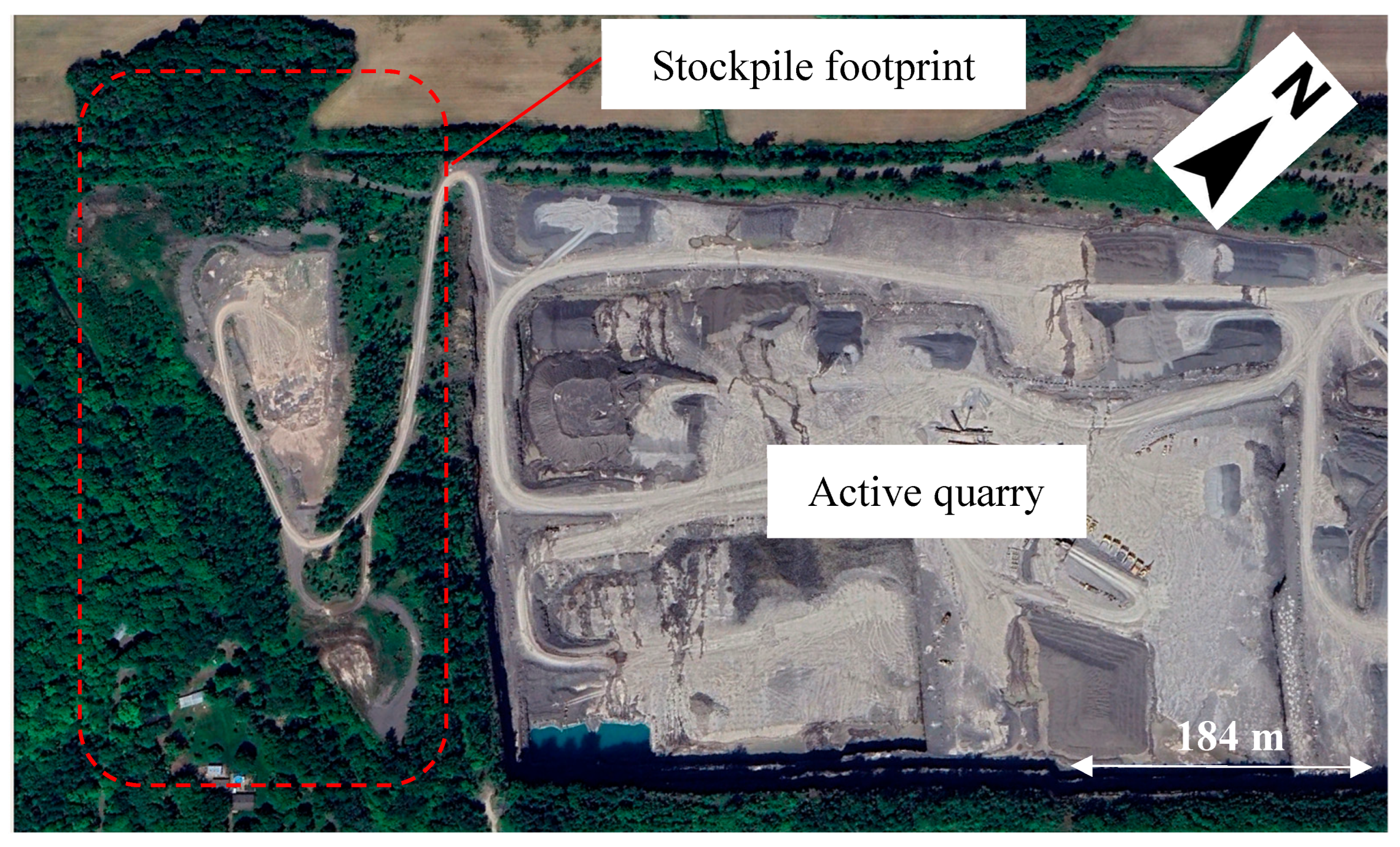
Figure 2.
Oblique view of the stockpile showing the 2023 landslide scar (outlined in red) (Image source: Google Earth, imagery © 2025 Airbus; imagery date: June 2025).
Figure 2.
Oblique view of the stockpile showing the 2023 landslide scar (outlined in red) (Image source: Google Earth, imagery © 2025 Airbus; imagery date: June 2025).
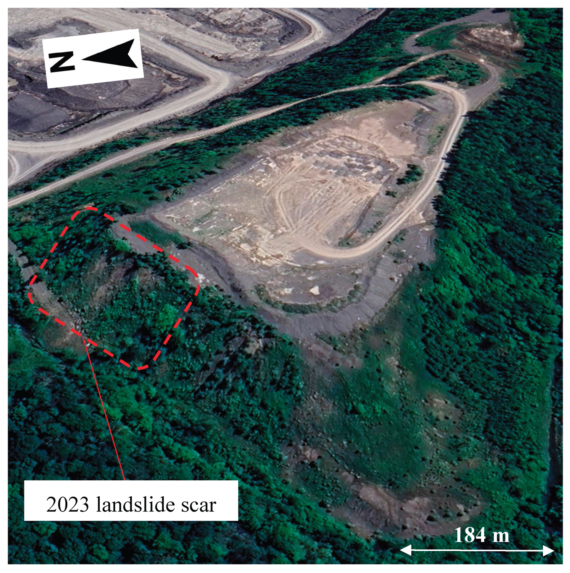
Figure 3.
Aerial photographs of the pile captured in spring 2025, showing the 2023 landslide scar and the stabilizing blocks placed at the toe. The dashed lines outline the two main failure zones: Zone A corresponds to the larger and more active portion of the slide, while Zone B represents a smaller and shallower failure to the east.
Figure 3.
Aerial photographs of the pile captured in spring 2025, showing the 2023 landslide scar and the stabilizing blocks placed at the toe. The dashed lines outline the two main failure zones: Zone A corresponds to the larger and more active portion of the slide, while Zone B represents a smaller and shallower failure to the east.
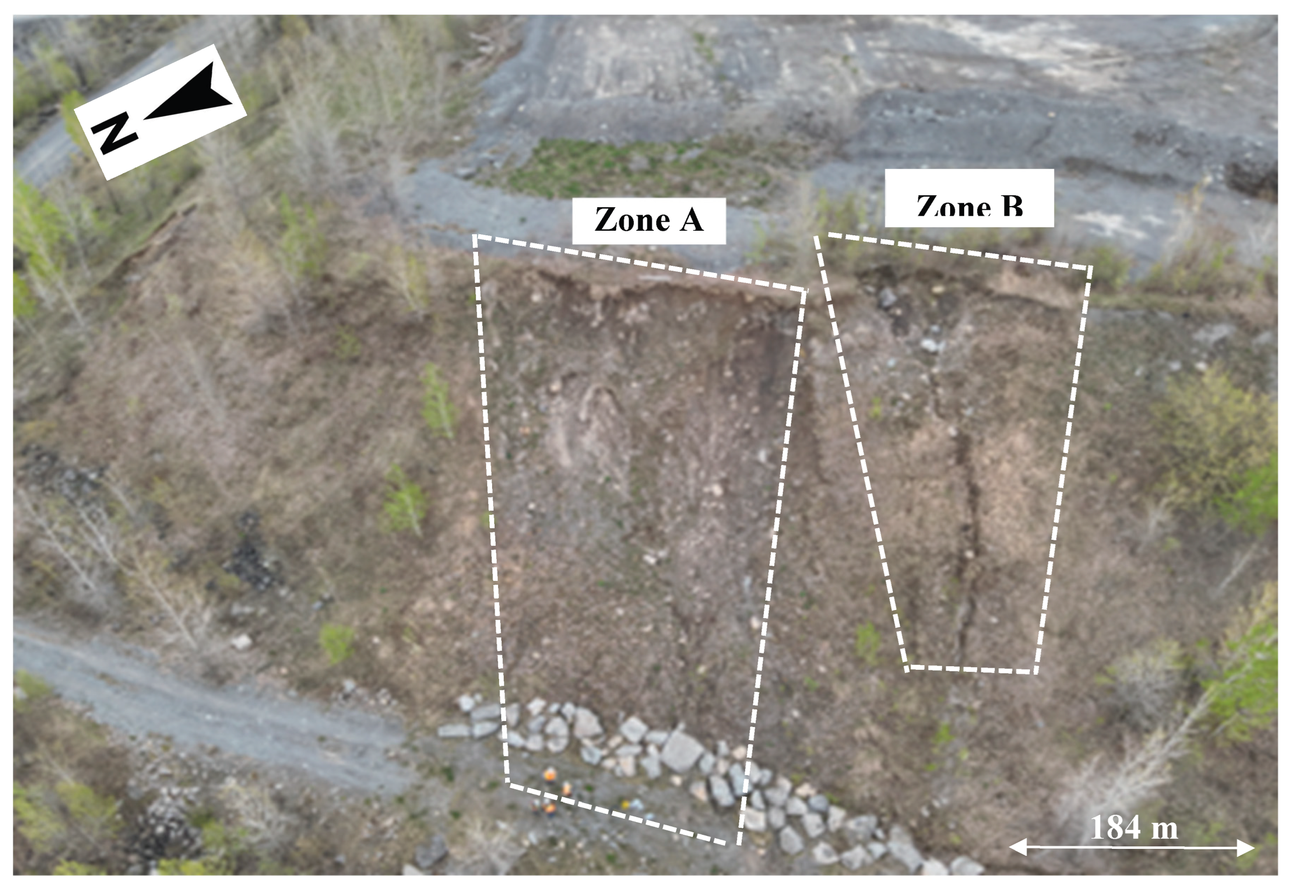
Figure 4.
(a) Point-cloud model acquired in October 2022 prior to failure, (b) point-cloud model acquired in April 2023 following the failure.
Figure 4.
(a) Point-cloud model acquired in October 2022 prior to failure, (b) point-cloud model acquired in April 2023 following the failure.
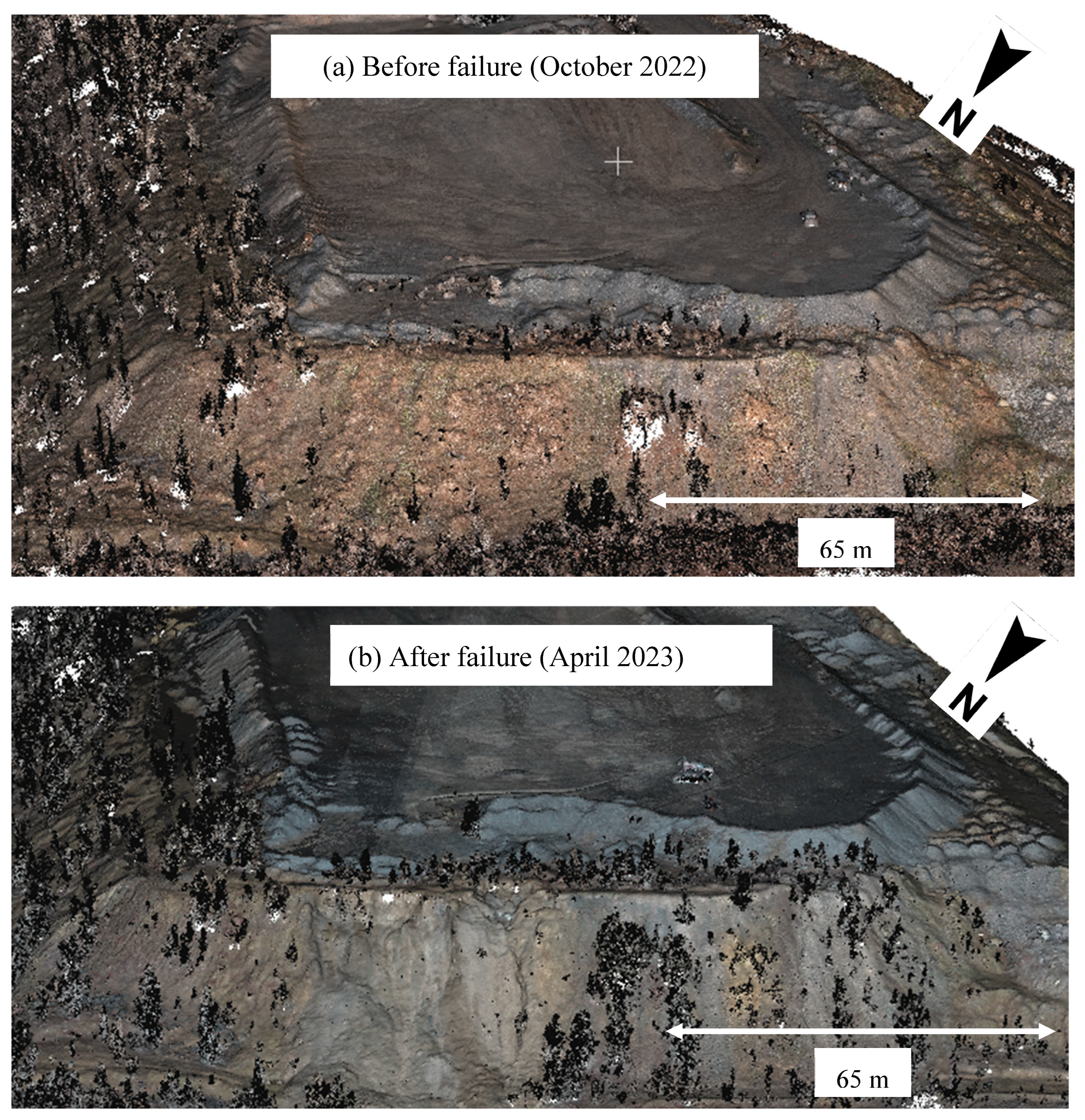
Figure 5.
Absolute C2C distance map showing the topographic changes between the October pre-failure and post-failure surveys.
Figure 5.
Absolute C2C distance map showing the topographic changes between the October pre-failure and post-failure surveys.
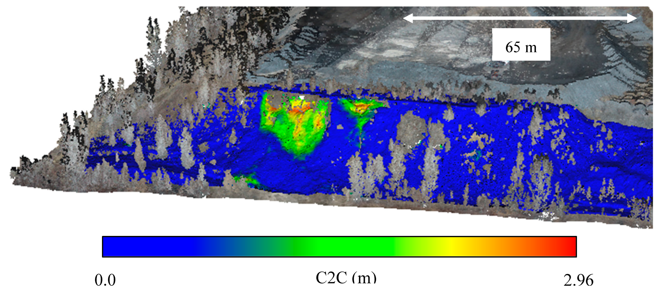
Figure 6.
C2C displacement results for the studied pile: (a) Zone A with peak displacement of 2.84 m and (b) Zone B with peak displacement of 2.76 m.
Figure 6.
C2C displacement results for the studied pile: (a) Zone A with peak displacement of 2.84 m and (b) Zone B with peak displacement of 2.76 m.
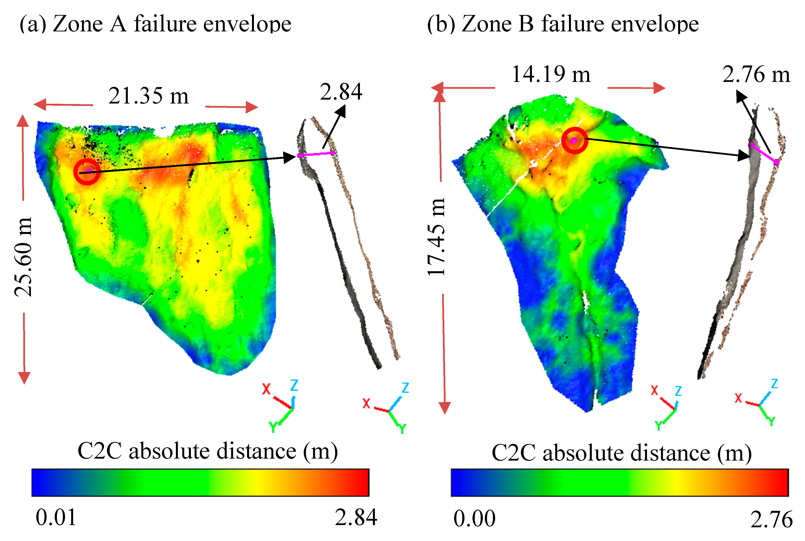
Figure 7.
Subdivision of the study area into three zones (Zone 1, Zone 2, and Zone 3) performed prior to vegetation filtering to optimize data processing, reduce computation time, and improve the precision of subsequent analyses.
Figure 7.
Subdivision of the study area into three zones (Zone 1, Zone 2, and Zone 3) performed prior to vegetation filtering to optimize data processing, reduce computation time, and improve the precision of subsequent analyses.
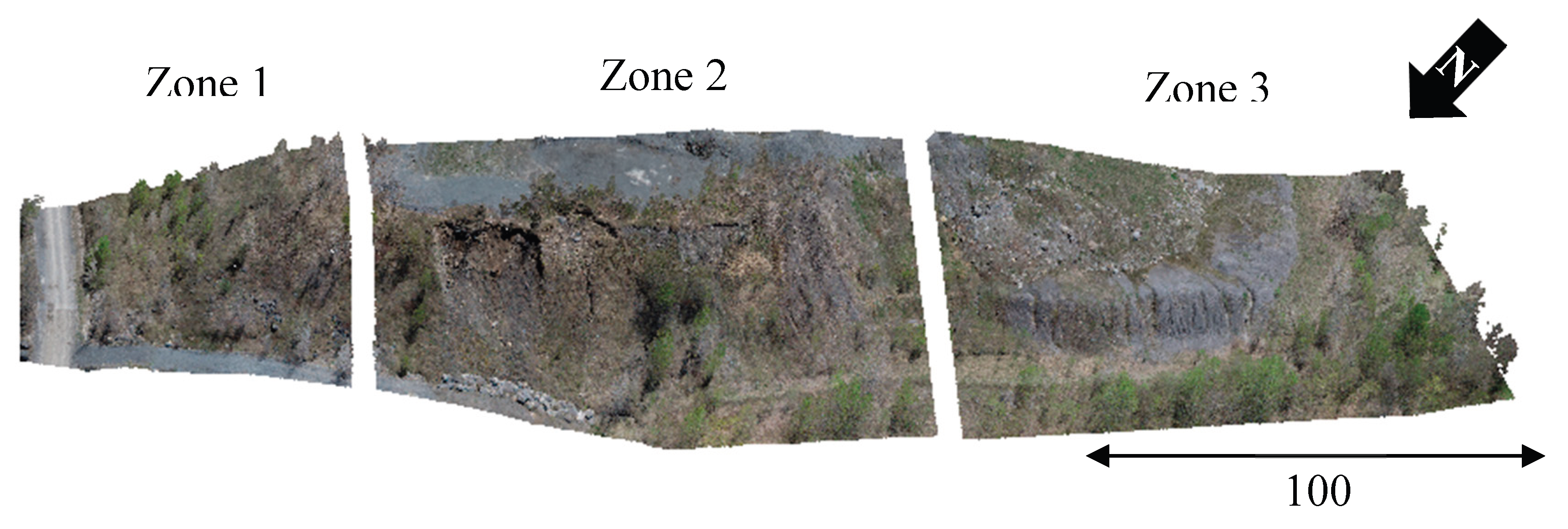
Figure 8.
Example of vegetation-filtering results using the CANUPO classifier. (a) Initial point cloud containing both vegetation and ground, (b) vegetation class, and (c) ground class retained for further analyses.
Figure 8.
Example of vegetation-filtering results using the CANUPO classifier. (a) Initial point cloud containing both vegetation and ground, (b) vegetation class, and (c) ground class retained for further analyses.
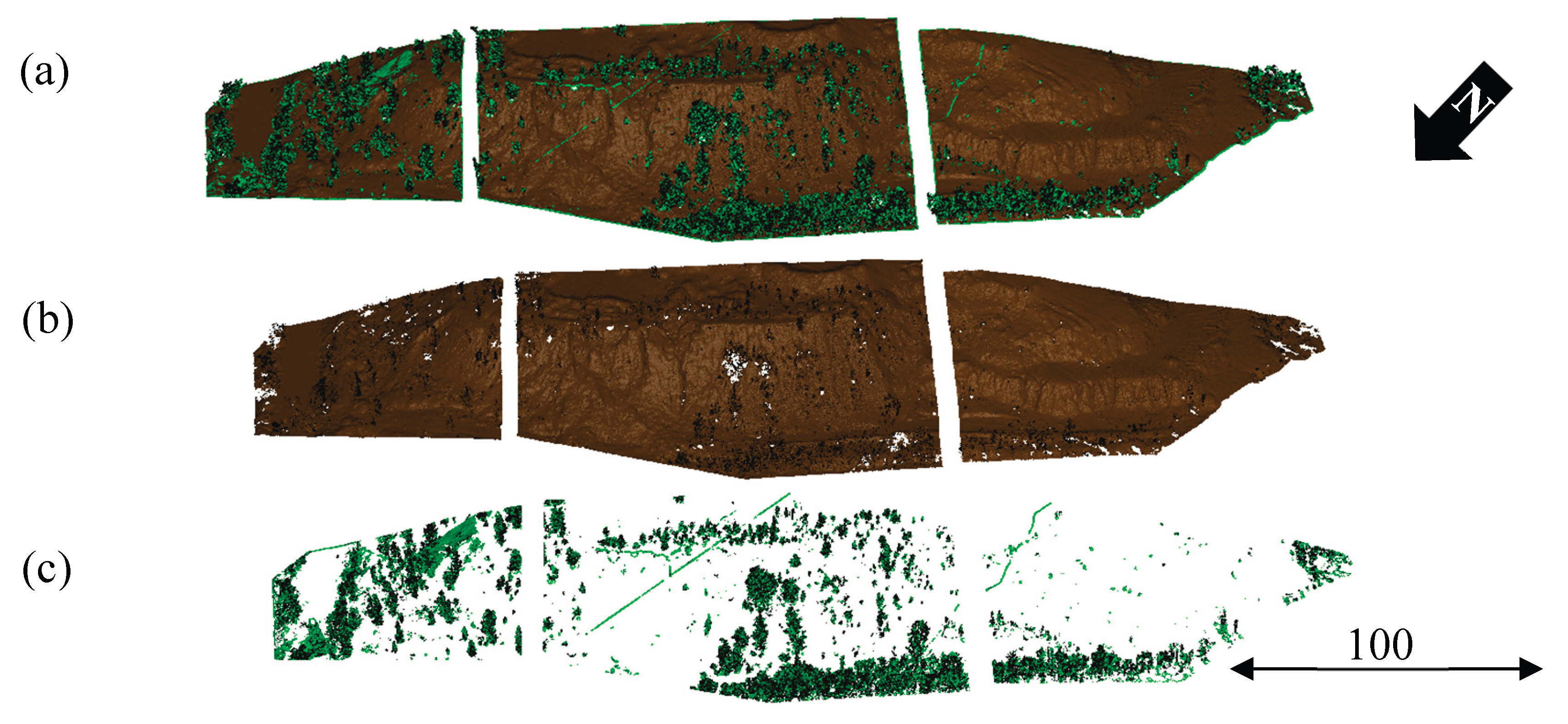
Figure 9.
Example of the evolution of C2C distance distribution curves during successive R-ICP iterations for Zone 1 between the November 2024 and May 2025 datasets.
Figure 9.
Example of the evolution of C2C distance distribution curves during successive R-ICP iterations for Zone 1 between the November 2024 and May 2025 datasets.
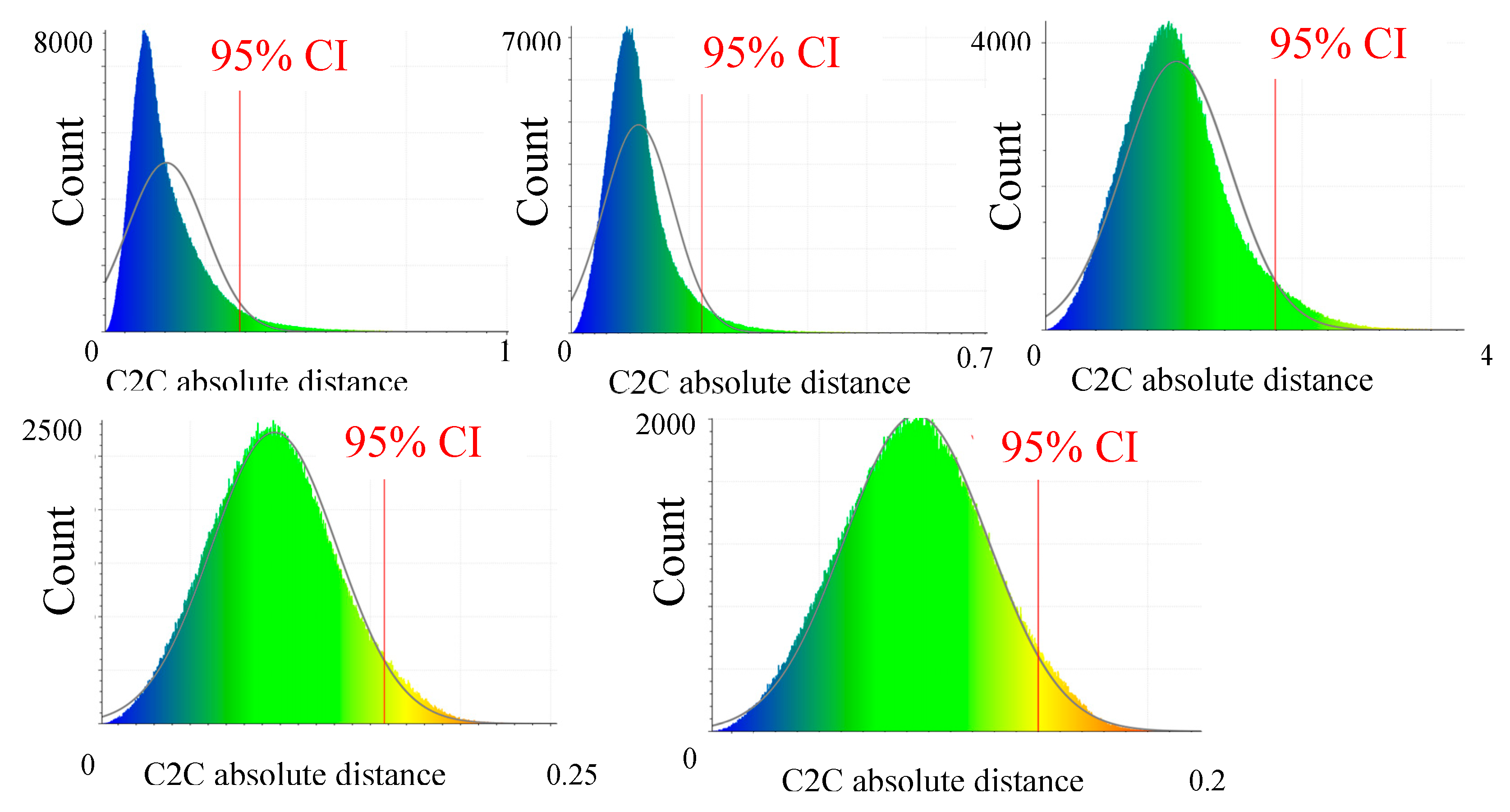
Figure 10.
Spatial evolution of C2C absolute distance maps during successive R-ICP iterations for Zone 1 between the November 2024 and May 2025 datasets.
Figure 10.
Spatial evolution of C2C absolute distance maps during successive R-ICP iterations for Zone 1 between the November 2024 and May 2025 datasets.
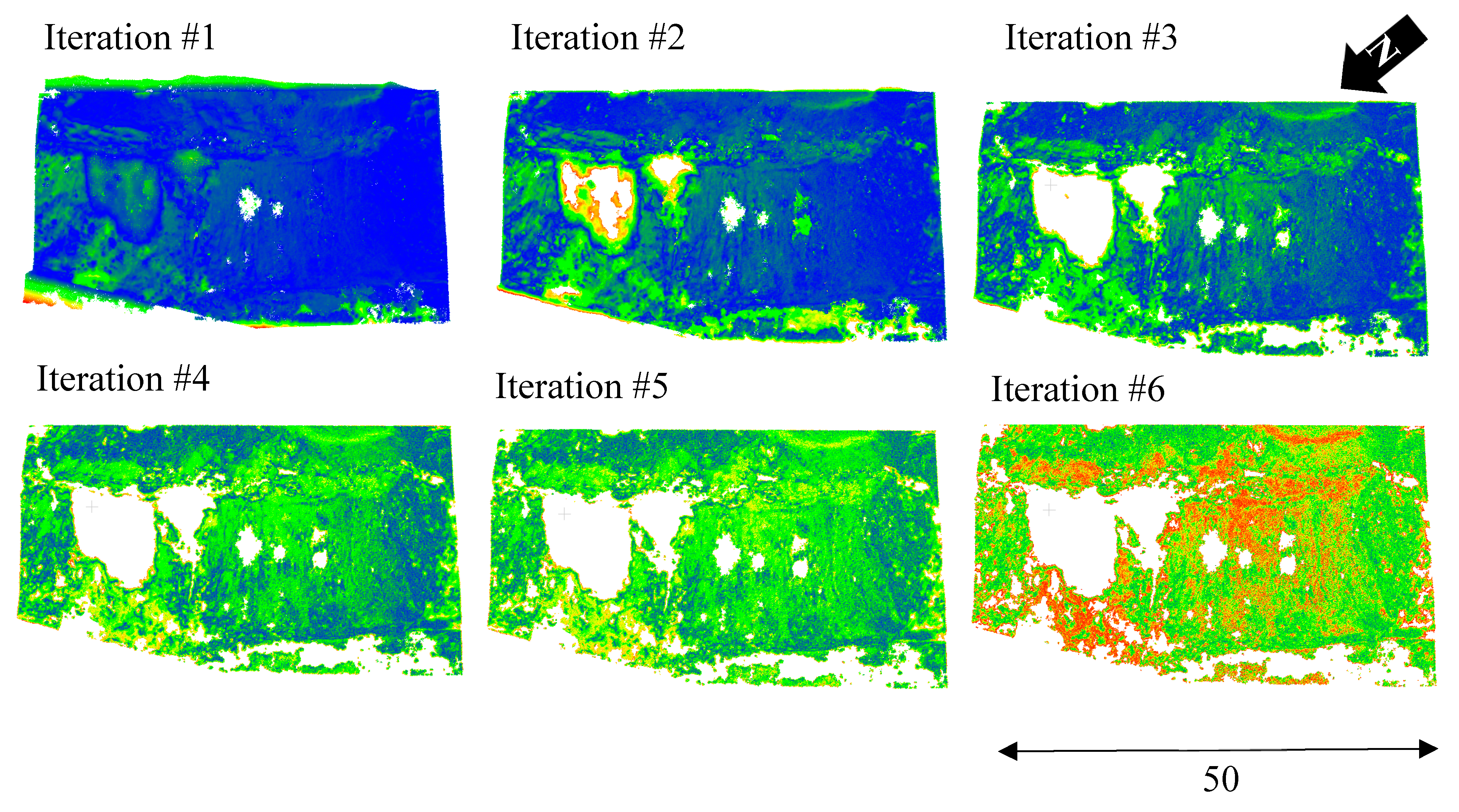
Figure 11.
Evolution of the mean, standard deviation, and 95% confidence interval (CI) of C2C distances during successive R-ICP iterations, for the example zone, showing progressive stabilization and convergence toward optimal alignment.
Figure 11.
Evolution of the mean, standard deviation, and 95% confidence interval (CI) of C2C distances during successive R-ICP iterations, for the example zone, showing progressive stabilization and convergence toward optimal alignment.
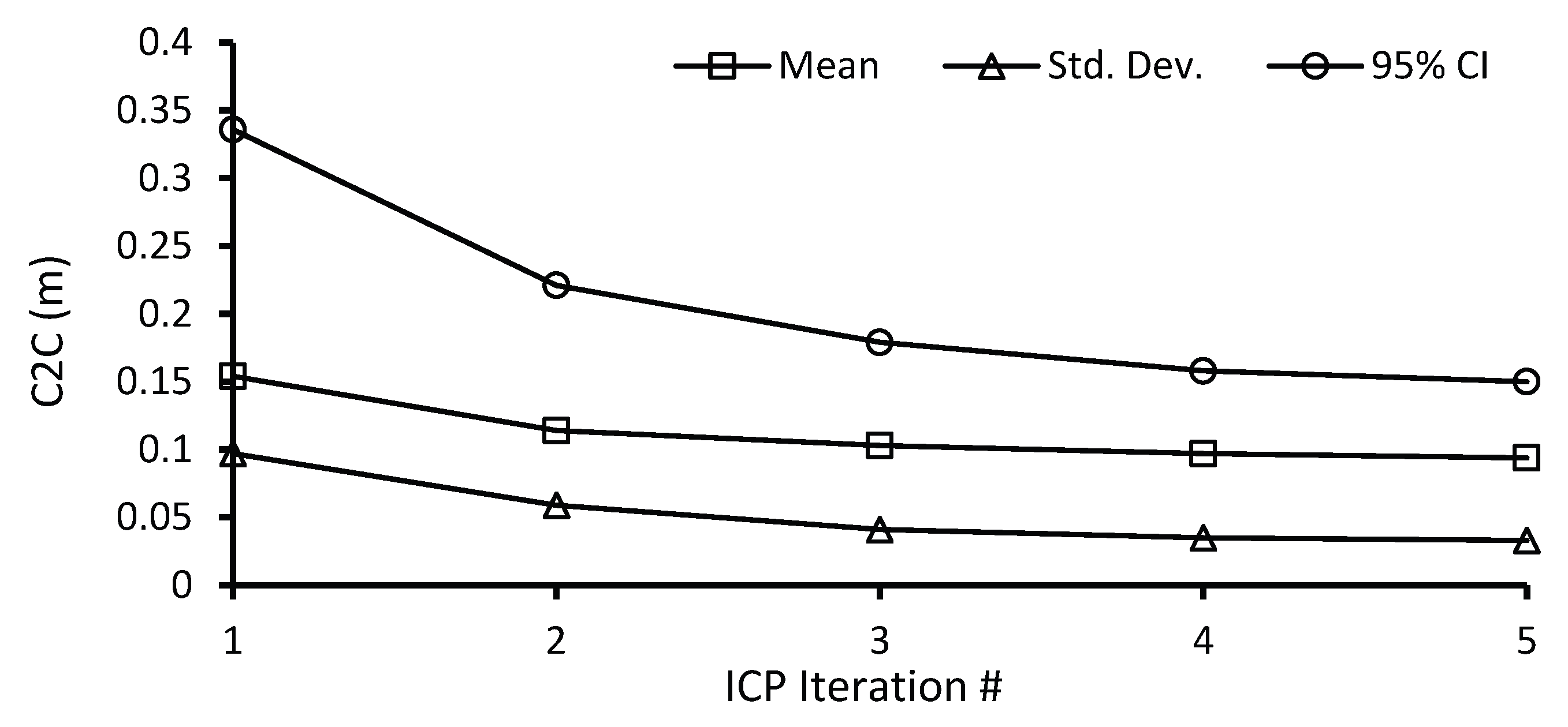
Figure 12.
Influence of surface geometry and acquisition conditions on beam-footprint error (σB): (a) spatial distribution of surface dip, and (b) variation of σB as a function of incidence angle for different acquisition distances.
Figure 12.
Influence of surface geometry and acquisition conditions on beam-footprint error (σB): (a) spatial distribution of surface dip, and (b) variation of σB as a function of incidence angle for different acquisition distances.
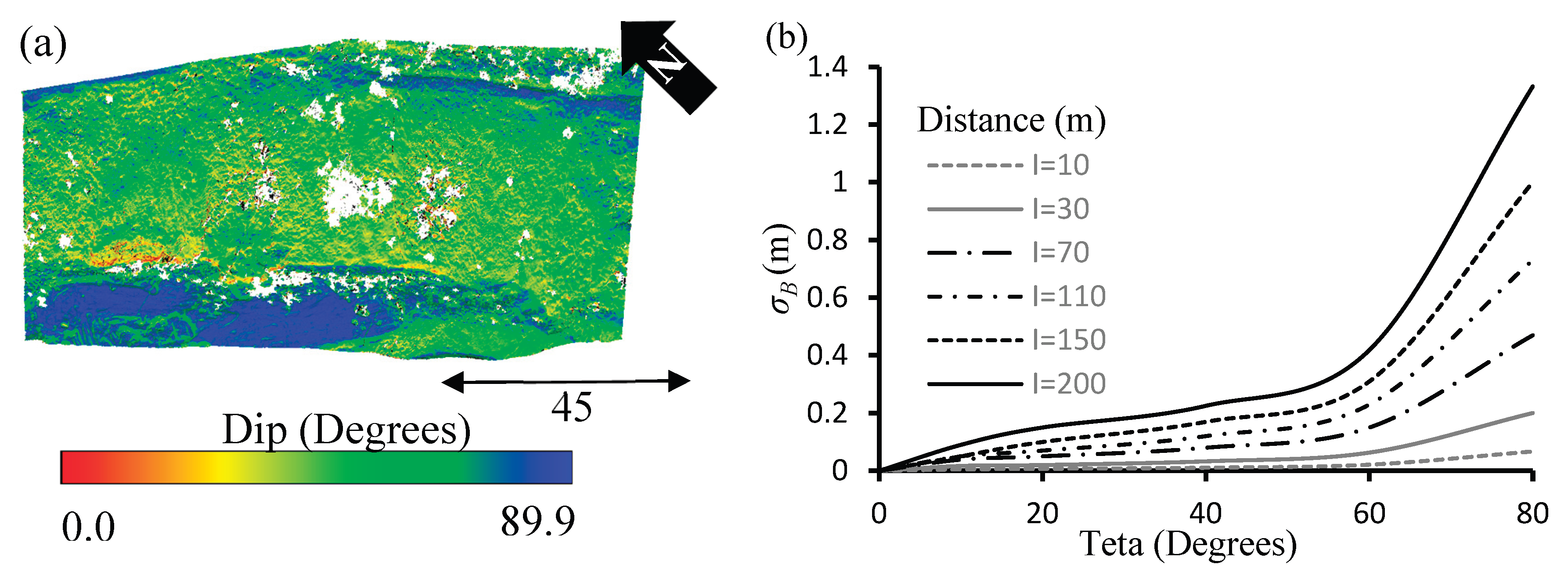
Figure 13.
C2C absolute distance measurements illustrating surface evolution between fall 2022 and spring 2023.
Figure 13.
C2C absolute distance measurements illustrating surface evolution between fall 2022 and spring 2023.
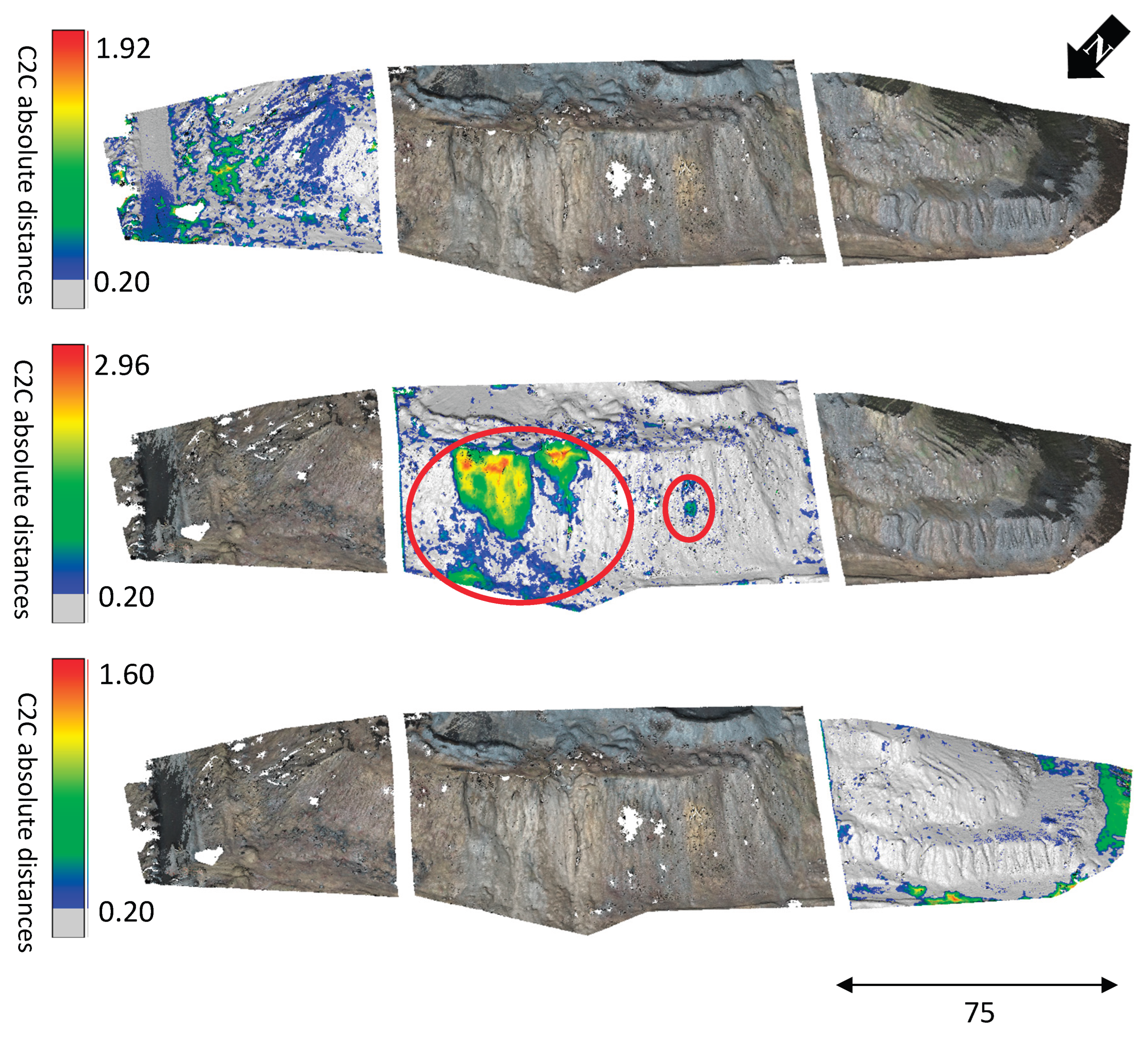
Figure 14.
C2C absolute distance measurements illustrating surface evolution between spring 2023 and fall 2023.
Figure 14.
C2C absolute distance measurements illustrating surface evolution between spring 2023 and fall 2023.
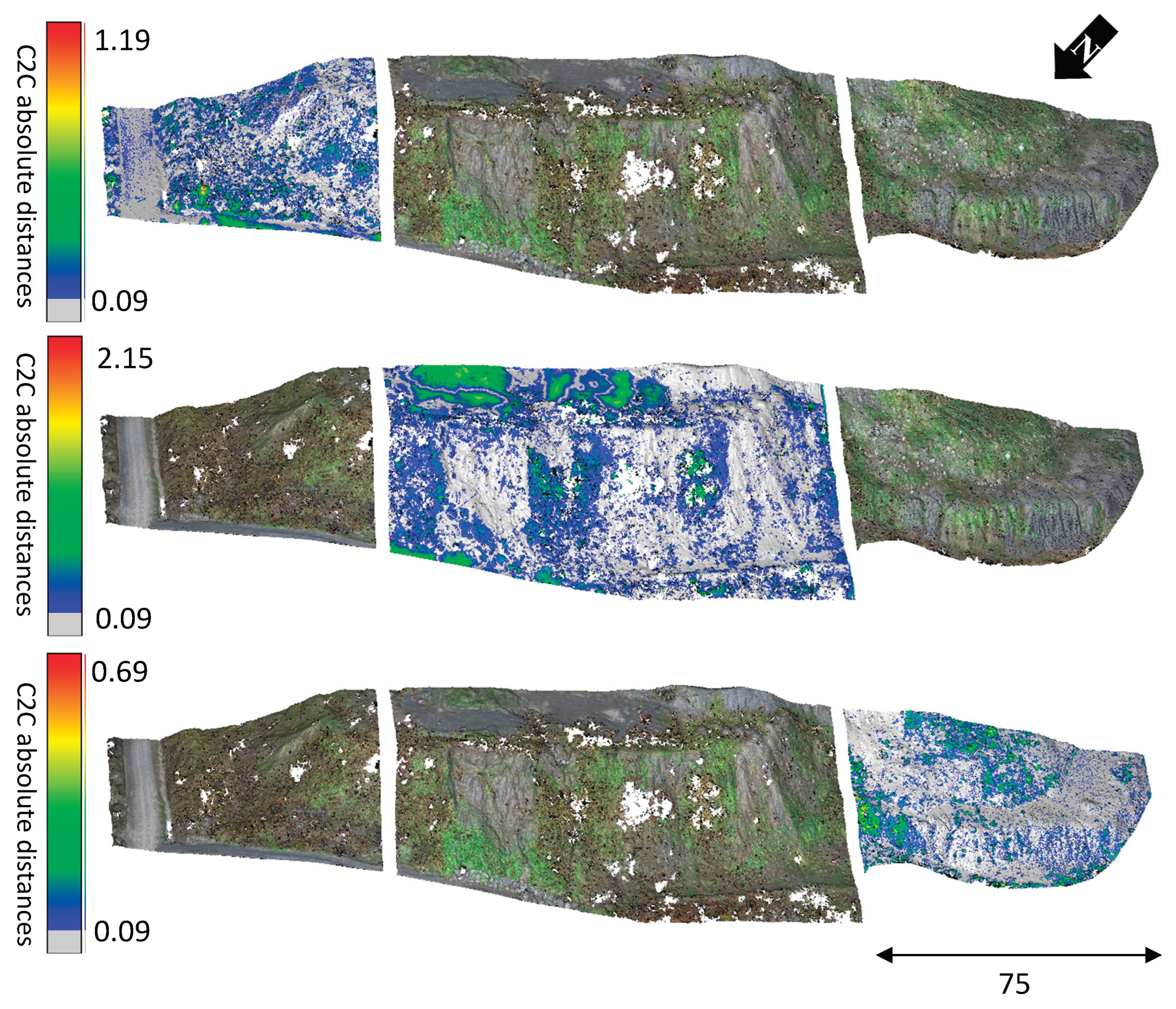
Figure 15.
C2C absolute distance measurements illustrating surface evolution between fall 2023 and spring 2024.
Figure 15.
C2C absolute distance measurements illustrating surface evolution between fall 2023 and spring 2024.
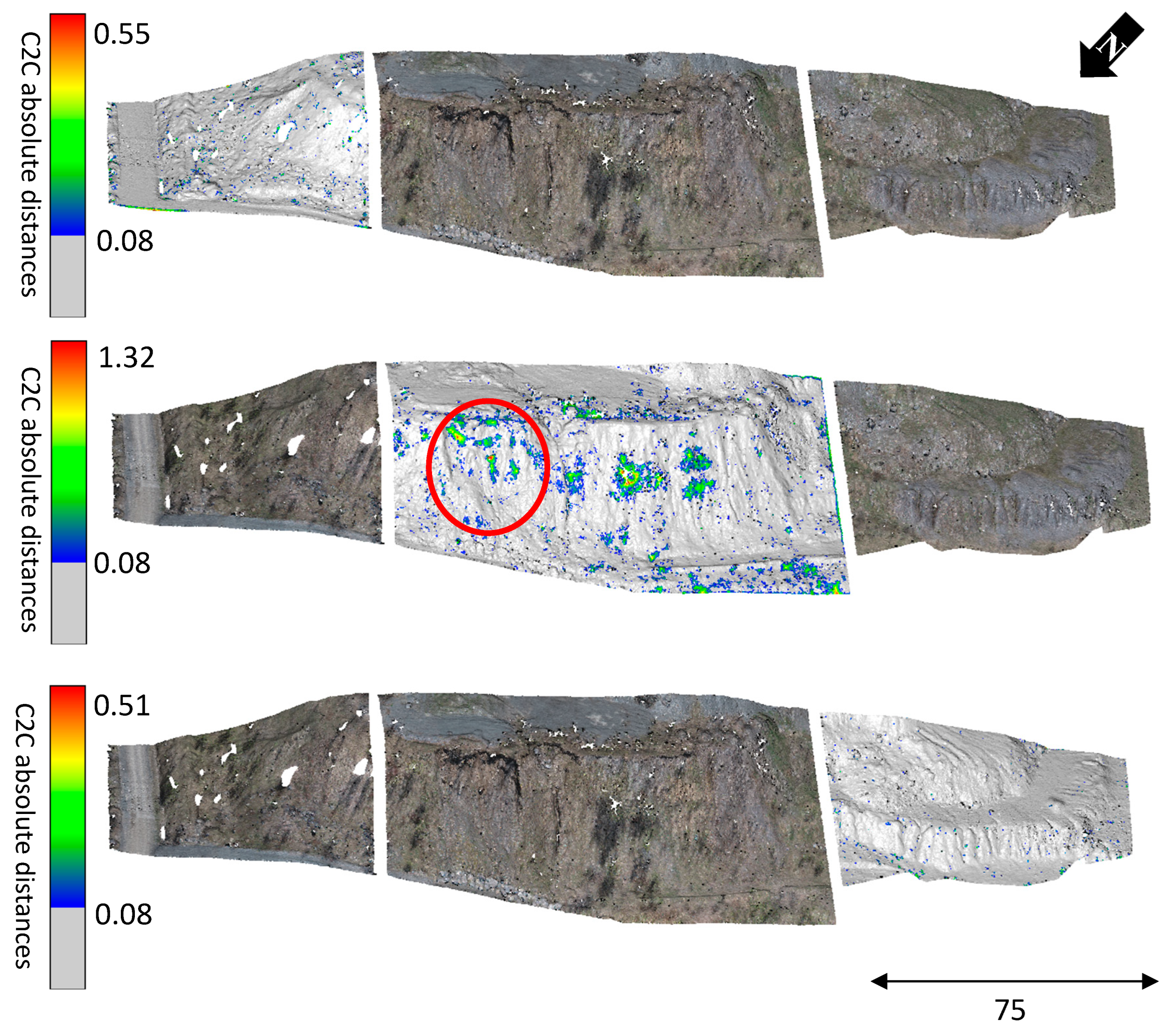
Figure 16.
C2C absolute distance measurements illustrating surface evolution between spring 2024 and fall 2024.
Figure 16.
C2C absolute distance measurements illustrating surface evolution between spring 2024 and fall 2024.
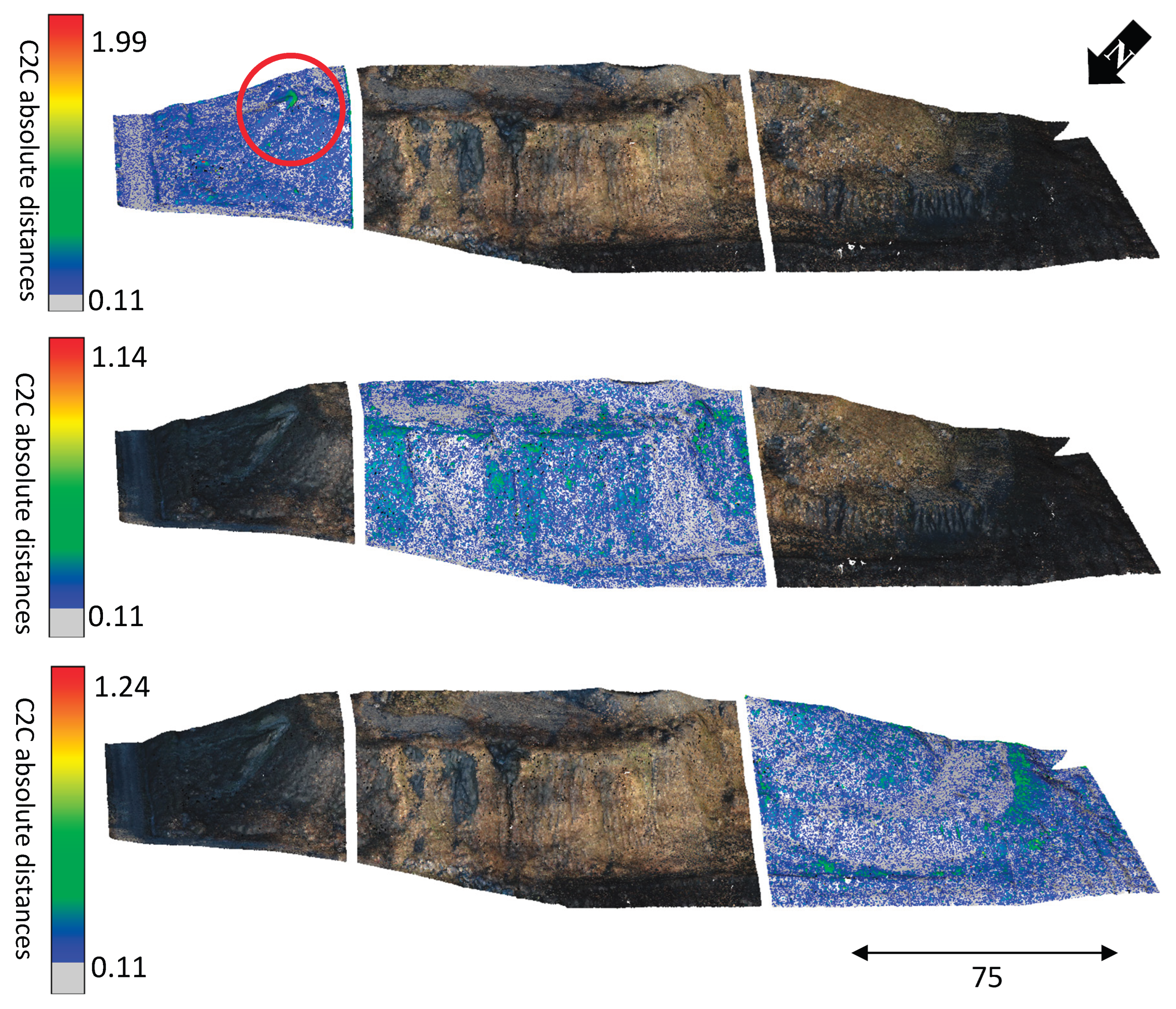
Figure 17.
C2C absolute distance measurements illustrating surface evolution between fall 2024 and spring 2025.
Figure 17.
C2C absolute distance measurements illustrating surface evolution between fall 2024 and spring 2025.
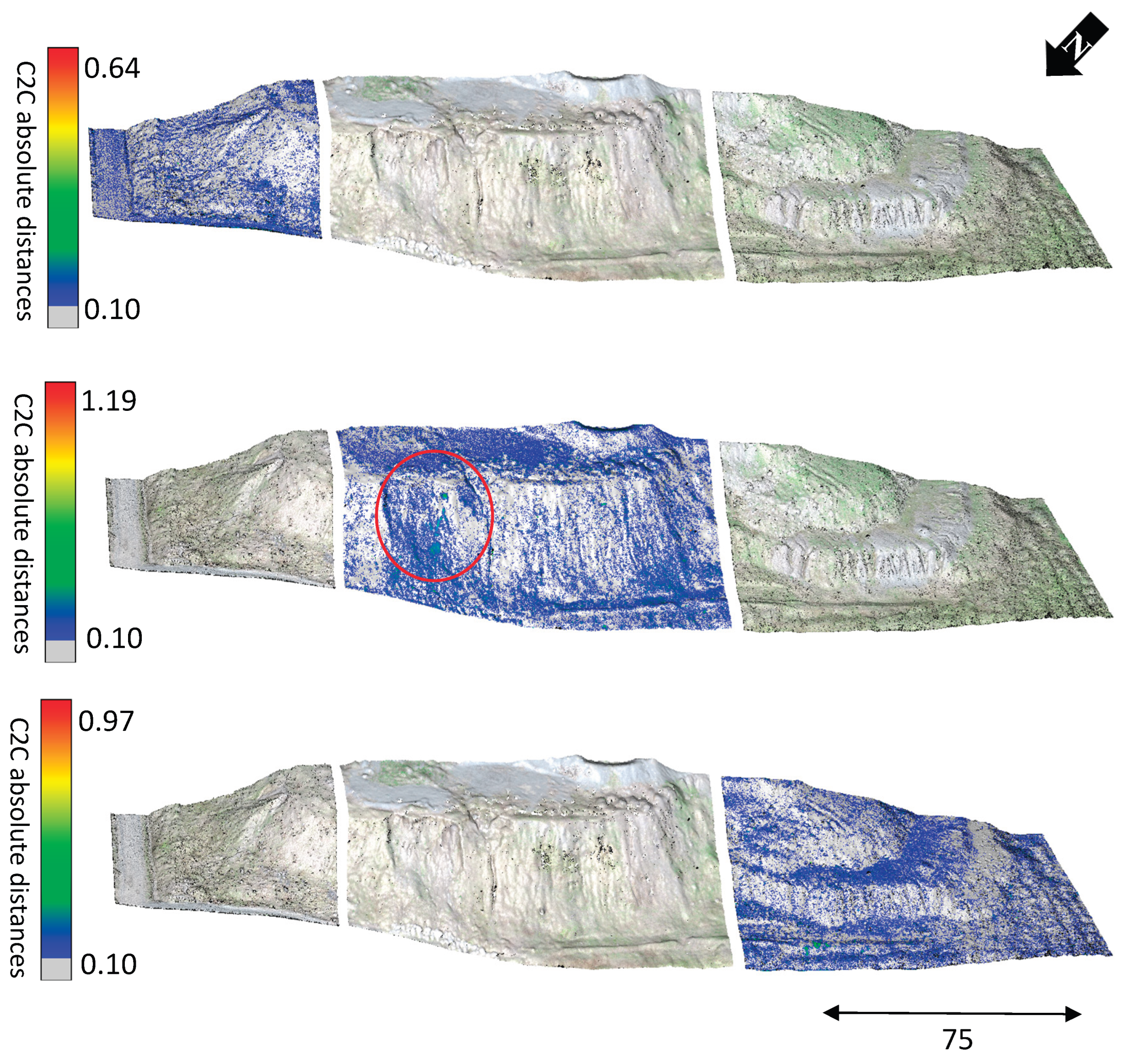
Figure 18.
Conceptual illustration of local roughness estimation from a 3D point cloud. (a) Definition of the spherical neighborhood of radius r centered on a reference point Pi, used to fit a local planar surface. (b) Computation of the roughness value Rr, i as the shortest distance between the reference point and the best-fit plane defined by its normal vector (after [40]).
Figure 18.
Conceptual illustration of local roughness estimation from a 3D point cloud. (a) Definition of the spherical neighborhood of radius r centered on a reference point Pi, used to fit a local planar surface. (b) Computation of the roughness value Rr, i as the shortest distance between the reference point and the best-fit plane defined by its normal vector (after [40]).
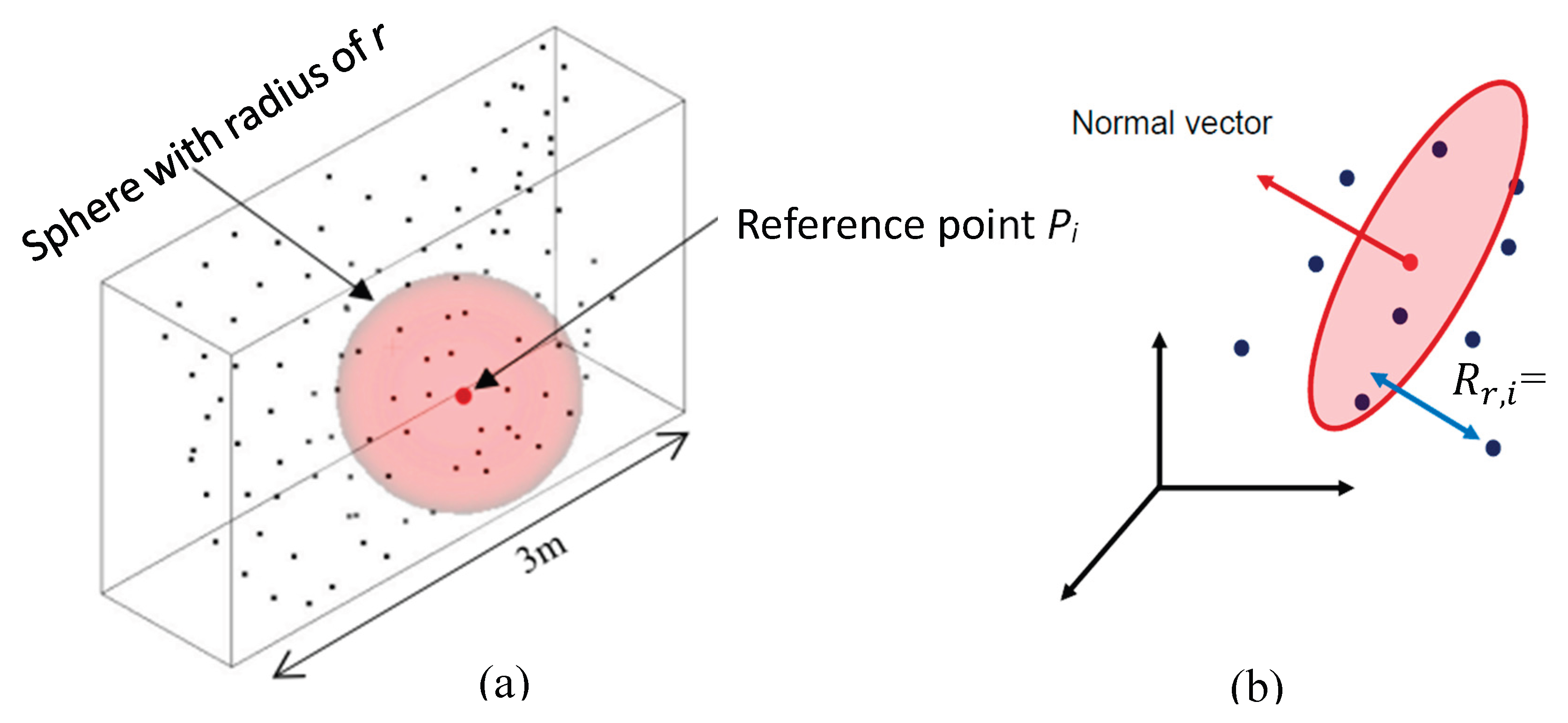
Figure 19.
Log–log plot of ξr versus r, highlighting the linear scale range representing illustrating the linear scale range and corresponding power-law fit.
Figure 19.
Log–log plot of ξr versus r, highlighting the linear scale range representing illustrating the linear scale range and corresponding power-law fit.
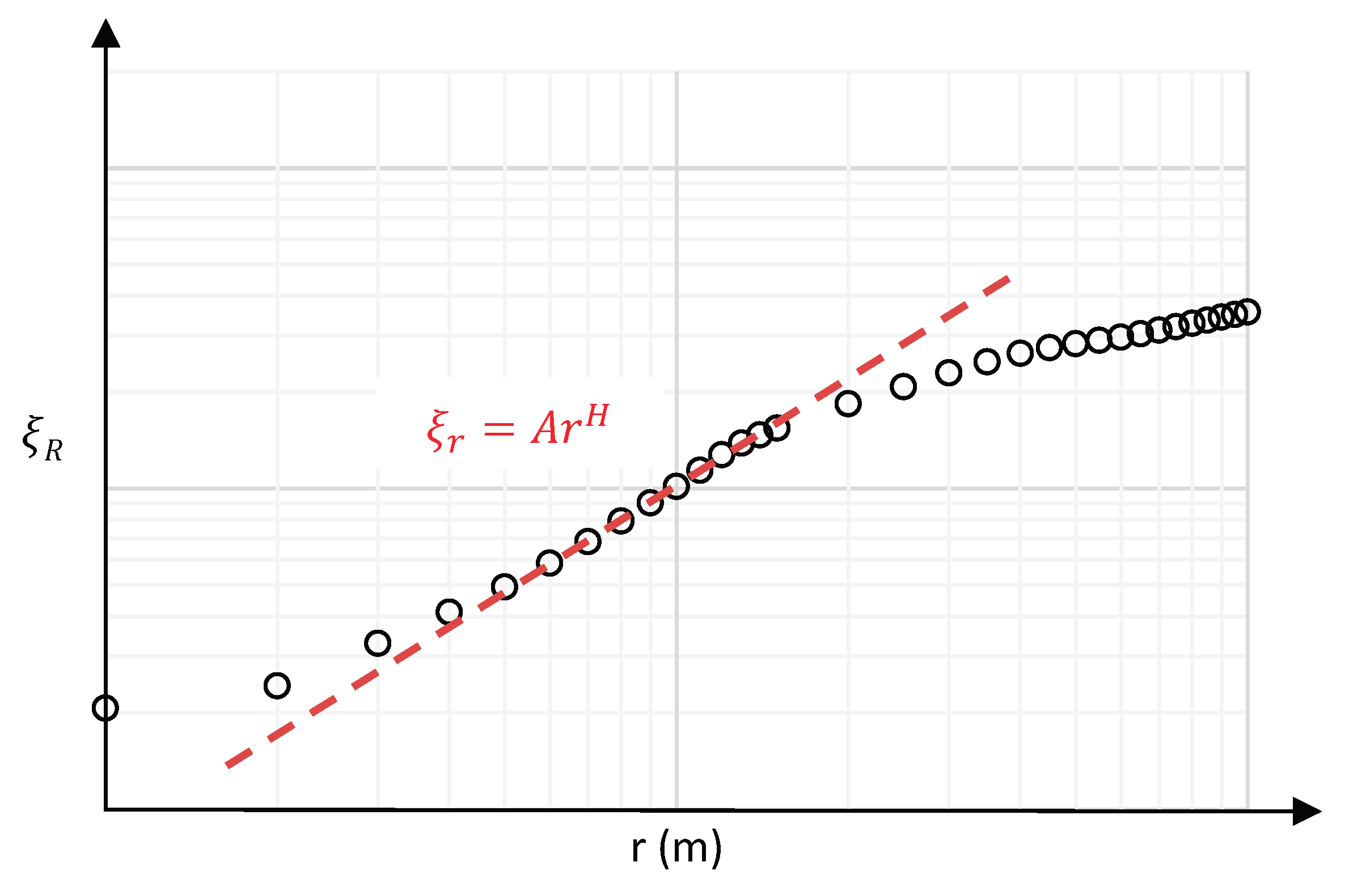
Figure 20.
irregular roughness patterns at failure zones.
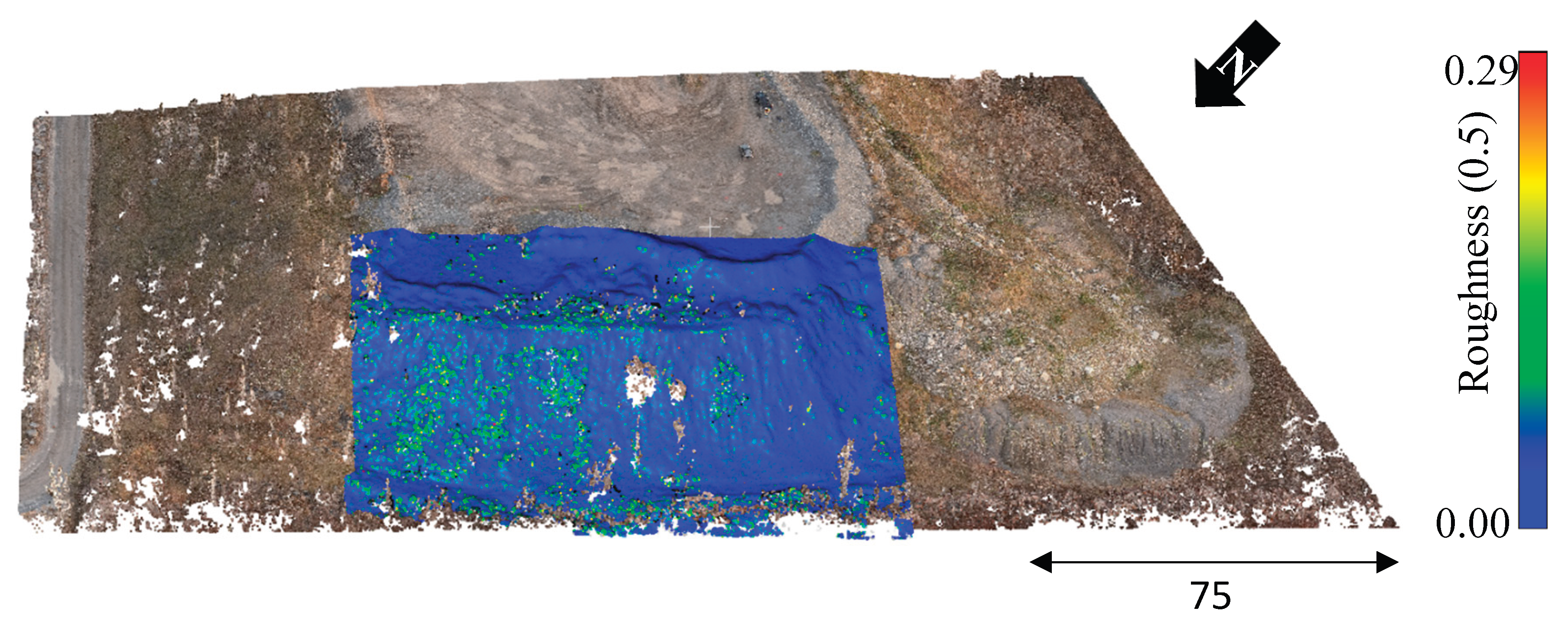
Figure 21.
Spatial distribution of the selected analysis sections, comprising one failure zone and three non-failure zones.
Figure 21.
Spatial distribution of the selected analysis sections, comprising one failure zone and three non-failure zones.
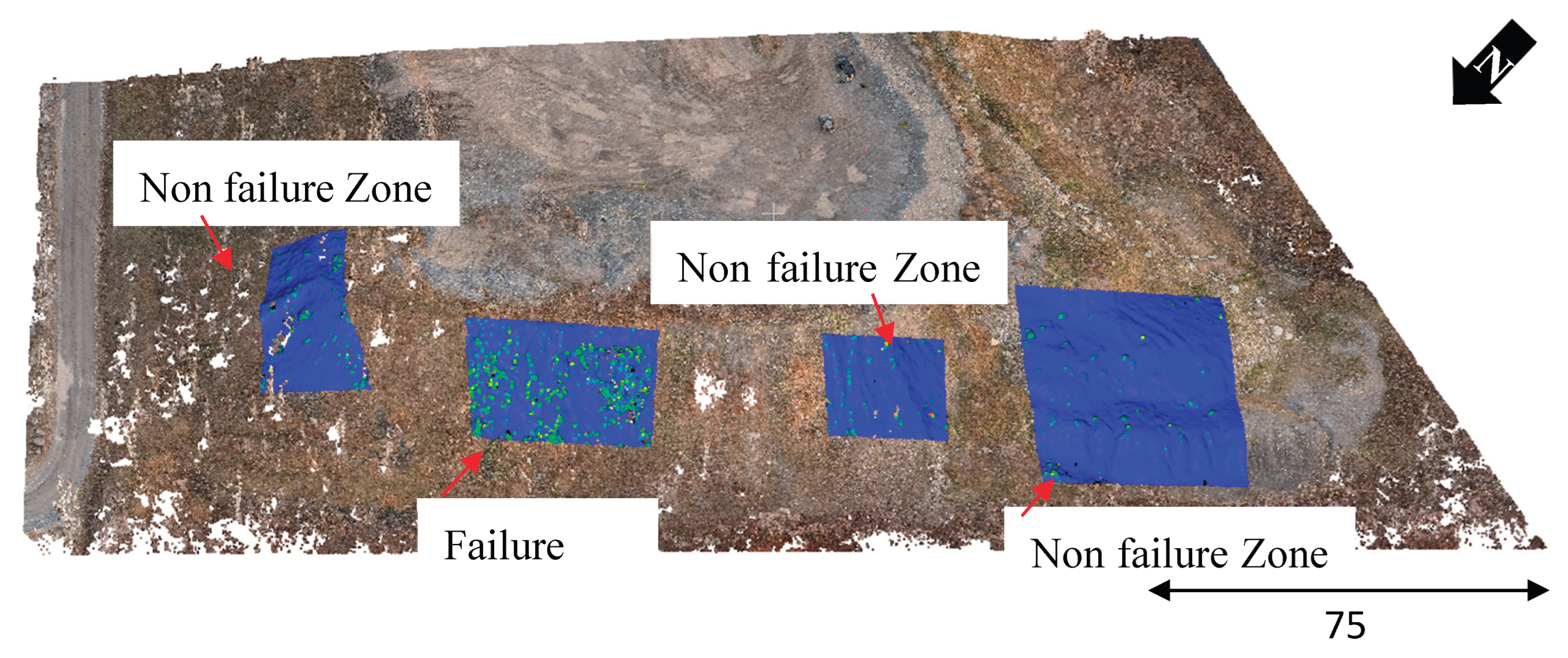
Figure 22.
multi-scale roughness analysis for the selected failure and non-failure zones over neighborhood radii ranging from 0.1 m to 10.
Figure 22.
multi-scale roughness analysis for the selected failure and non-failure zones over neighborhood radii ranging from 0.1 m to 10.
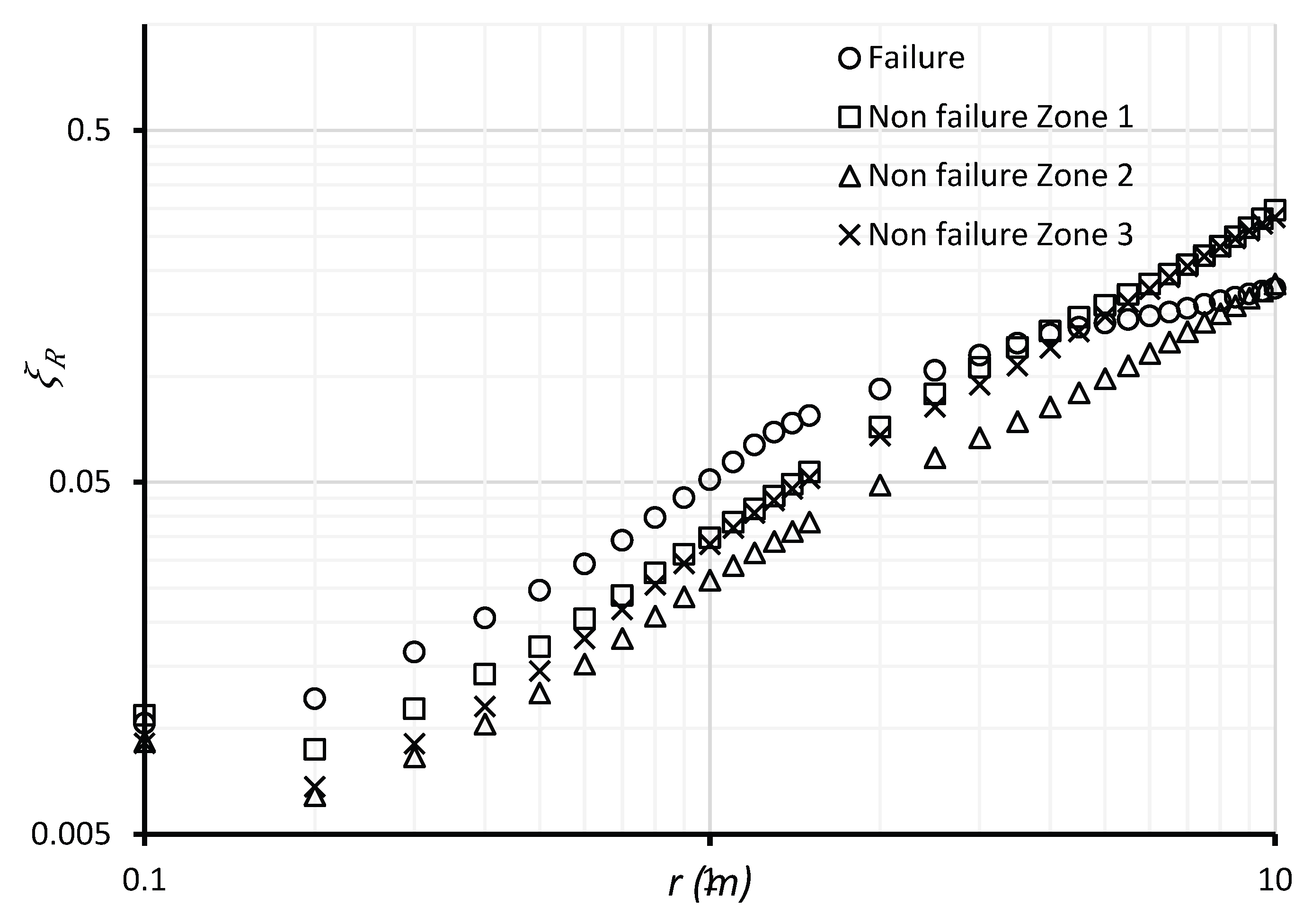
Figure 23.
Spatial distribution of the scale-dependent roughness indicator (A/D) computed using a 5 × 5 m grid. (a) A/D map over the analyzed slope section. (b) Elevated A/D values form coherent patterns that align with the identified failure zone.
Figure 23.
Spatial distribution of the scale-dependent roughness indicator (A/D) computed using a 5 × 5 m grid. (a) A/D map over the analyzed slope section. (b) Elevated A/D values form coherent patterns that align with the identified failure zone.
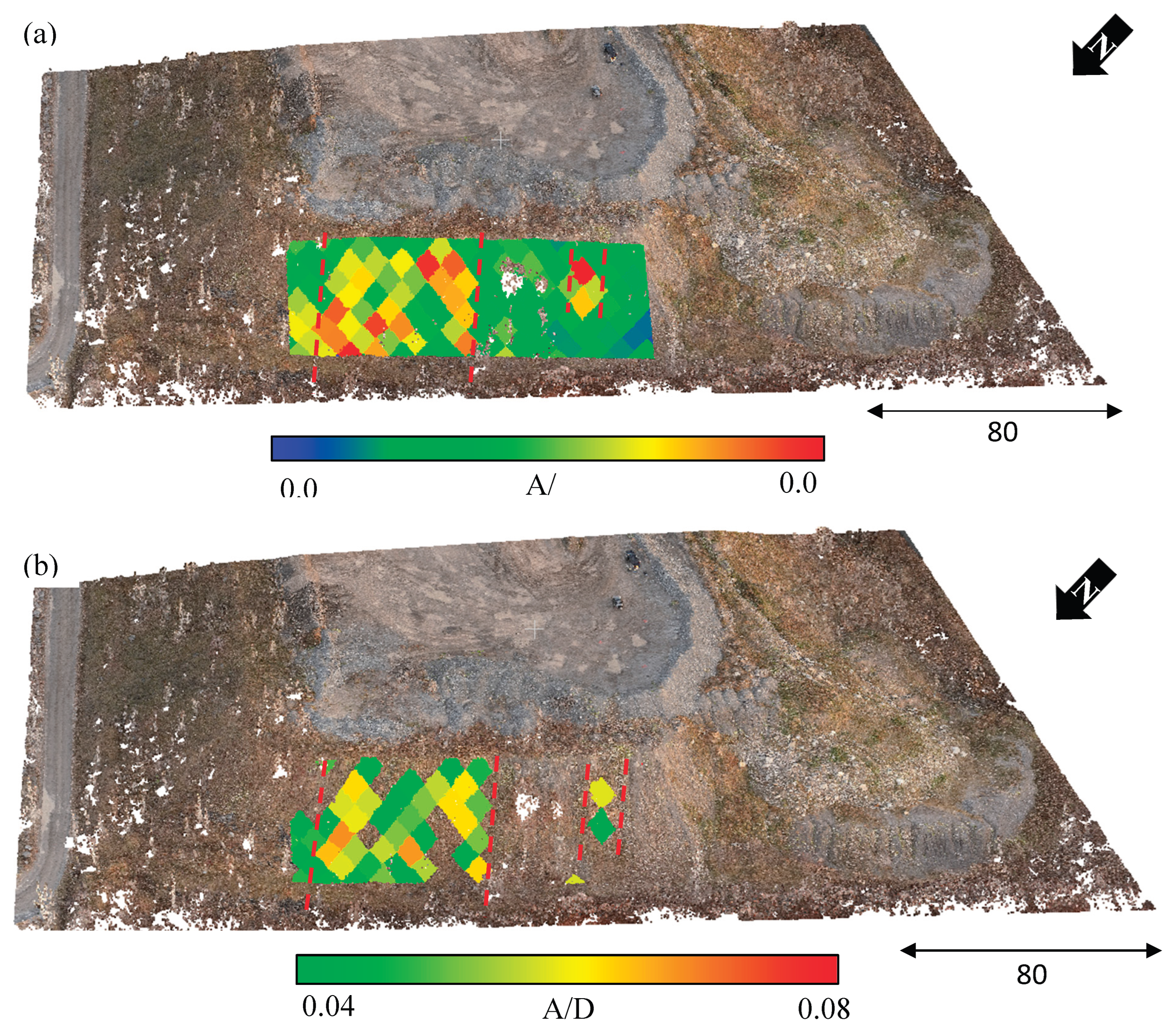
Figure 24.
Spatial distribution of the scale-dependent roughness indicator (A/D) computed using a 1 × 1 m grid.
Figure 24.
Spatial distribution of the scale-dependent roughness indicator (A/D) computed using a 1 × 1 m grid.
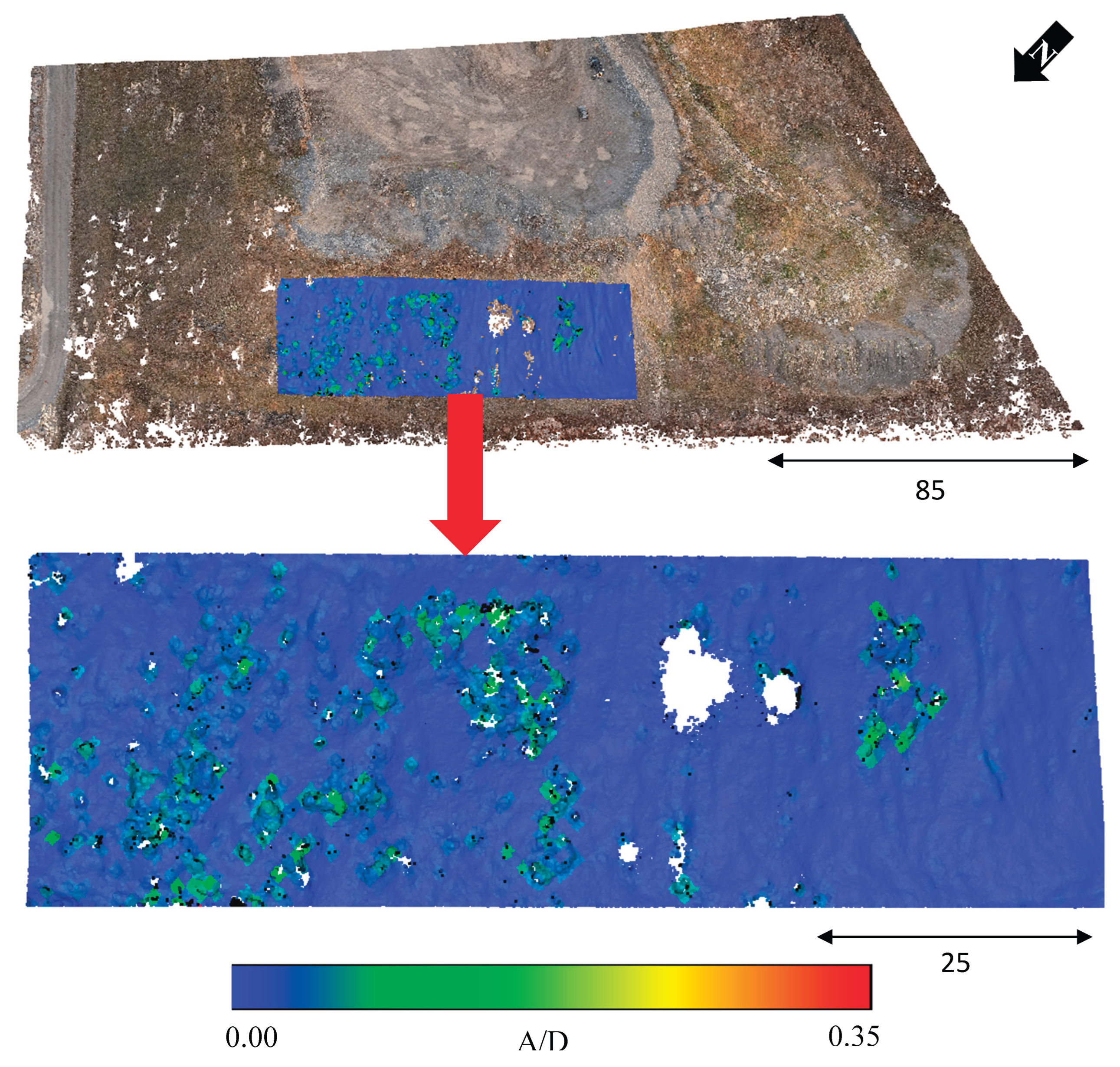
Figure 25.
Temporal evolution of scale-dependent roughness (ξᵣ) within the selected failure zone for multiple survey dates. (a) Multi-scale roughness trends over the full range of measurement radii. (b) Zoomed view of the consistent linear scale range between 1 and 2 m used for comparative analysis across time.
Figure 25.
Temporal evolution of scale-dependent roughness (ξᵣ) within the selected failure zone for multiple survey dates. (a) Multi-scale roughness trends over the full range of measurement radii. (b) Zoomed view of the consistent linear scale range between 1 and 2 m used for comparative analysis across time.
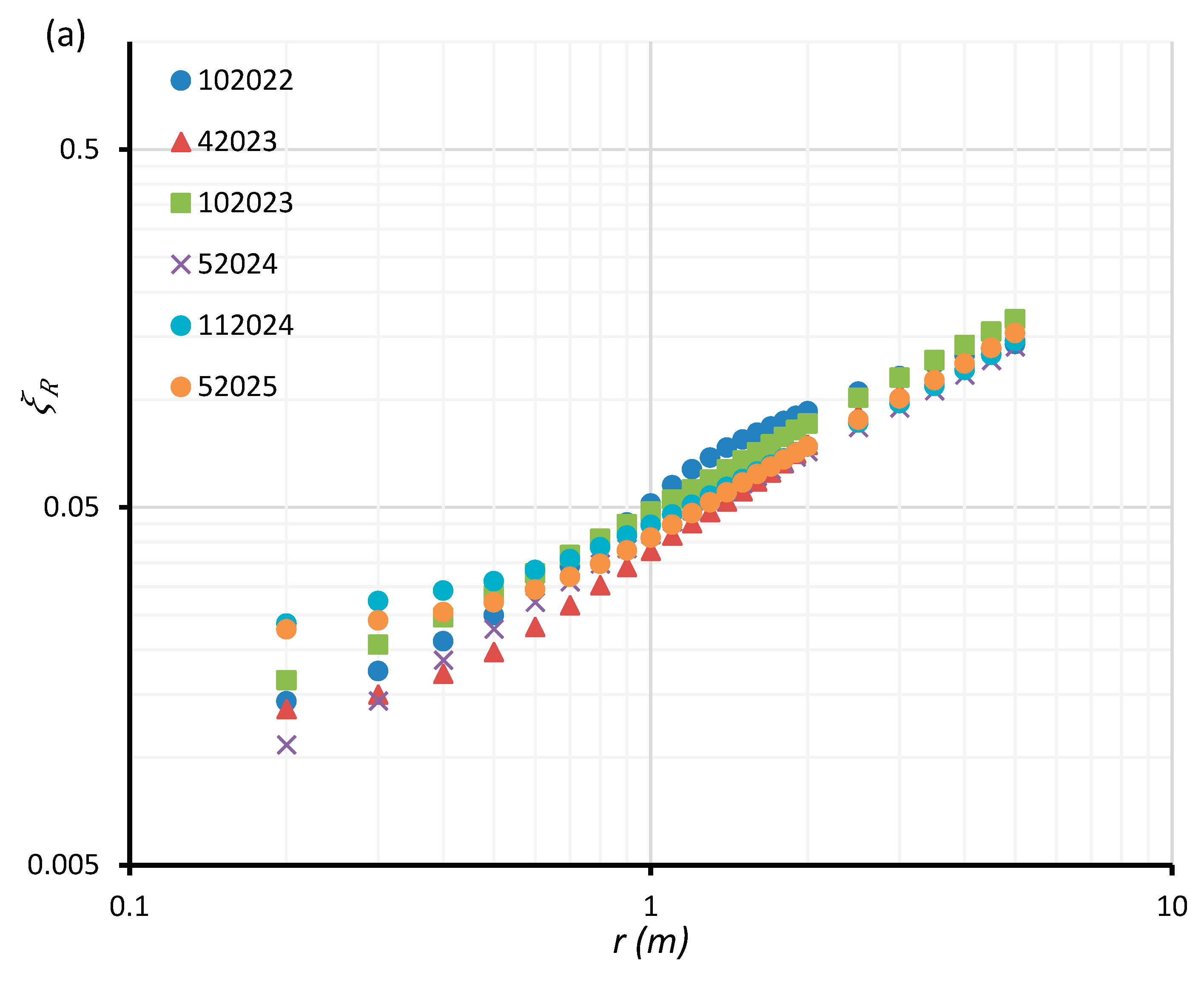
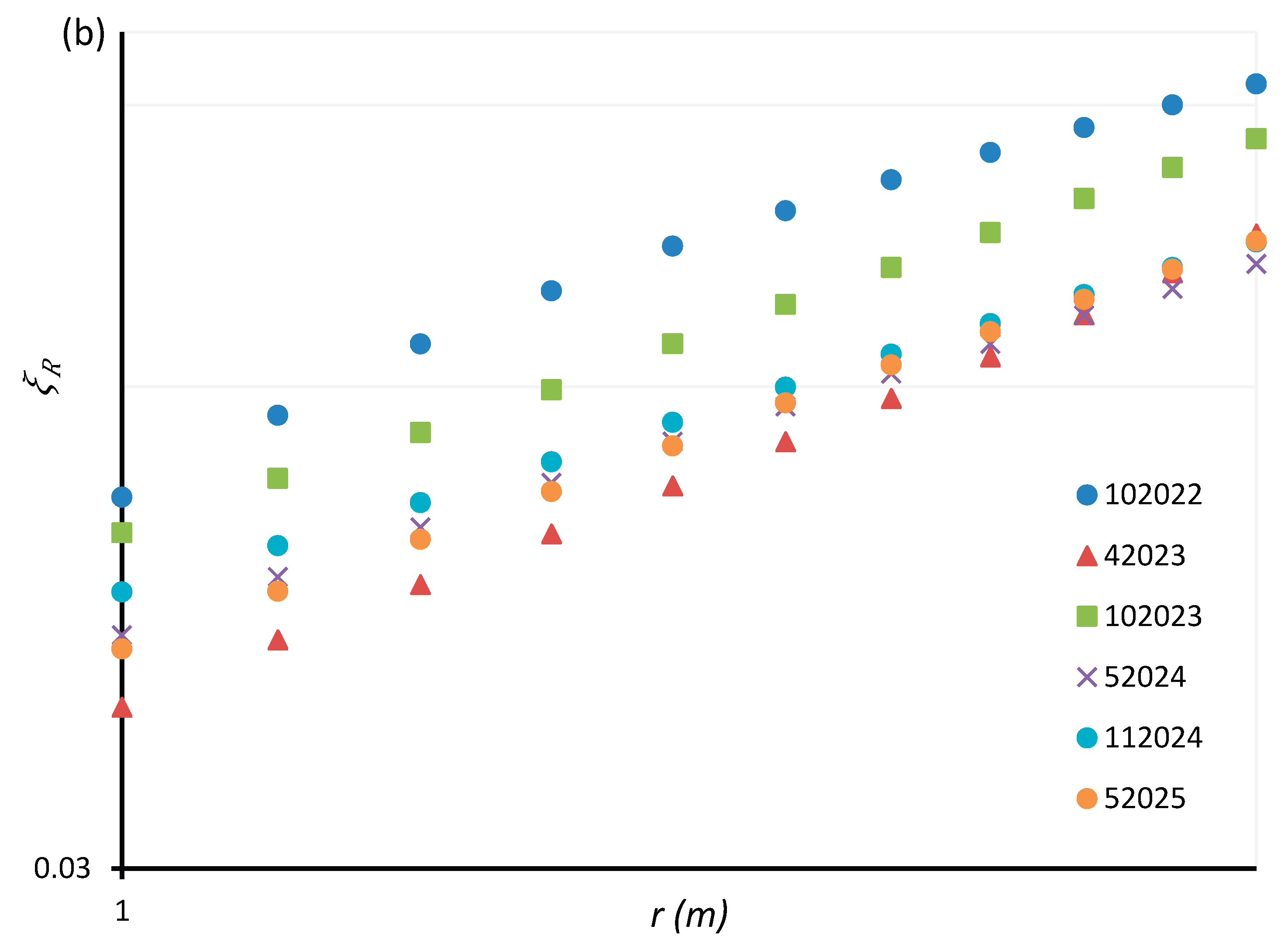
Figure 26.
Cloud-to-cloud (C2C) change detection results between successive survey epochs within the failure zone.
Figure 26.
Cloud-to-cloud (C2C) change detection results between successive survey epochs within the failure zone.
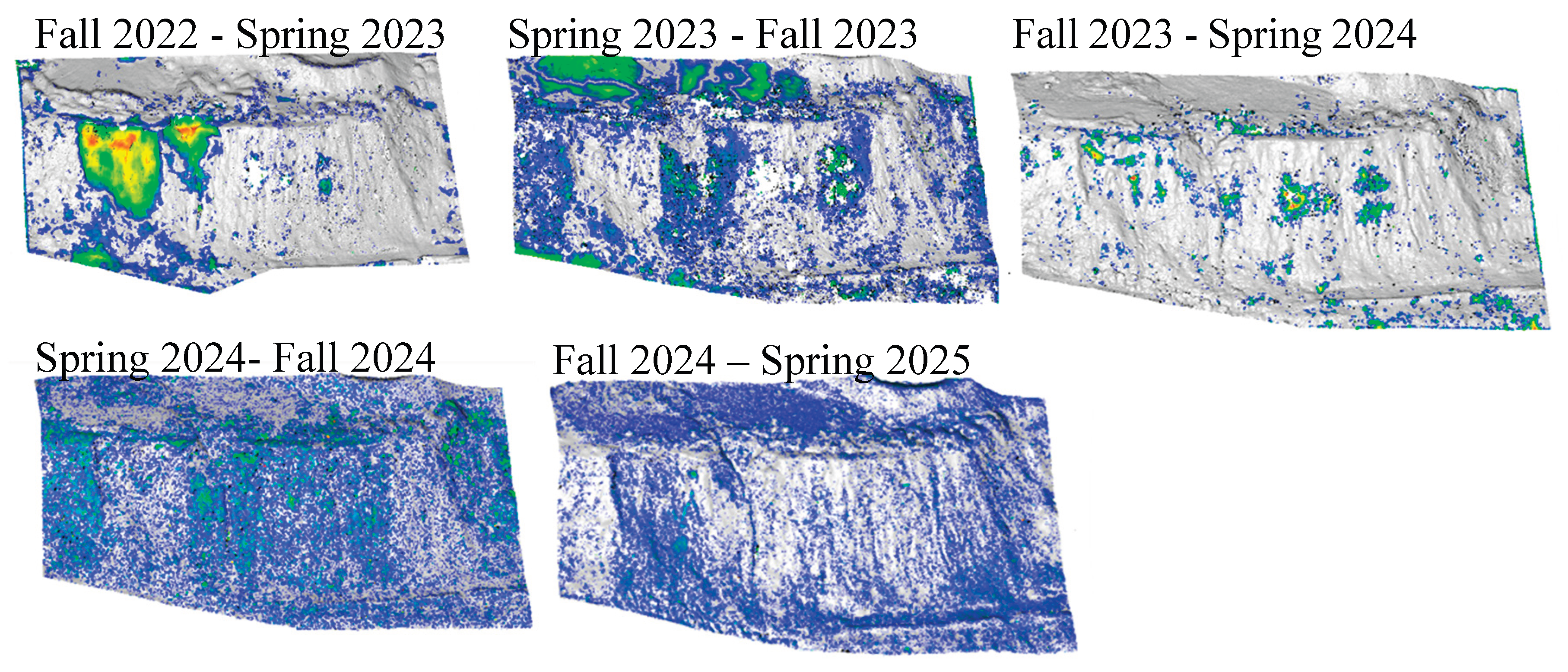

Table 1.
Overview of surveyed datasets.
| Sensor | Date | Average Point Spacing (m) |
|---|---|---|
| MAVIC 3E | Fall 2022 | 0.30 |
| Zenmuse L1 LiDAR | Fall 2023 | 0.11 |
| Zenmuse L1 LiDAR | Fall 2023 | 0.12 |
| Zenmuse L1 LiDAR | Spring 2024 | 0.17 |
| Zenmuse L1 LiDAR | Fall 2024 | 0.12 |
| Zenmuse L1 LiDAR | Spring 2025 | 0.12 |
Table 2.
Uncertainty components used in LoD calculations for LiDAR and photogrammetry.
| Error component | Zenmuse L1 | Mavic 3E |
|---|---|---|
| σtool | 3 cm @100m | 4.5 cm |
| σB / σPM | ~ 0.06 m | ~ 0.06m |
Table 3.
Estimated σC2C values derived from cloud-to-cloud distance analysis for each pair of survey epochs.
Table 3.
Estimated σC2C values derived from cloud-to-cloud distance analysis for each pair of survey epochs.
| Time interval | σC2C |
|---|---|
| Spring 2023 WRT Fall 2022 | ~ 20 cm |
| Fall 2023 WRT Spring 2023 | 8 – 9 cm |
| Spring 2024 WRT Fall 2023 | 7 – 8 cm |
| Fall 2024 WRT Spring 2024 | 10 – 11cm |
| Spring 2025 WRT Fall 2024 | 9 -10 cm |
Disclaimer/Publisher’s Note: The statements, opinions and data contained in all publications are solely those of the individual author(s) and contributor(s) and not of MDPI and/or the editor(s). MDPI and/or the editor(s) disclaim responsibility for any injury to people or property resulting from any ideas, methods, instructions or products referred to in the content. |
© 2026 by the authors. Licensee MDPI, Basel, Switzerland. This article is an open access article distributed under the terms and conditions of the Creative Commons Attribution (CC BY) license (http://creativecommons.org/licenses/by/4.0/).
Copyright: This open access article is published under a Creative Commons CC BY 4.0 license, which permit the free download, distribution, and reuse, provided that the author and preprint are cited in any reuse.


