Nonlinear Characteristics and Control Optimization of Giant Magneto Ultrasonic Transducers Under Random Excitation

Shen Guo; Jia Xu

doi:10.20944/preprints202607.0118.v1

Submitted:

30 June 2026

Posted:

02 July 2026

You are already at the latest version

Abstract

Ultrasonic technology is widely used in the precision machining of hard and brittle materials and giant magnetoelectric material has a broad application prospect in precision machining. Based on these, giant magnetostrictive ultrasonic transducer(GMUT) plays an important role in precision machining. The nonlinear dynamic characteristics of the magnetostrictive ultrasonic transducer have been studied with the aim of improving the accuracy of the transducer in this paper. Firstly, the nonlinear differential term is introduced to describe the hysteresis phenomenon, and the dynamic equations of GMUT are established. And then the nonlinear dynamic characteristics of the magnetostrictive ultrasonic transducer have been analyzed and the key parameters affecting the transducer have been obtained. Finally, the feedforward compensation fuzzy PID compound control scheme is designed and the simulation model is built. The simulation and experiment results show that the feedforward compensation fuzzy PID compound control strategy based on the results of nonlinear dynamics theory has high control precision.

Keywords:

giant magnetostrictive material

;

nonlinear dynamics

;

ultrasonic transducer

;

inverse compensation control

;

random excitation

Subject:

Engineering - Mechanical Engineering

Introduction

Hard and brittle materials, such as crystalline silicon, engineering ceramics, and composites, are characterized by high stability, high-temperature resistance, and corrosion resistance, offering broad application prospects in modern industries like aviation and aerospace. However, their processing difficulties often compromise part accuracy, limiting their practical use. Consequently, developing precision machining technologies for these materials has become a pressing challenge.

The most popular technique for machining hard and brittle materials is rotary ultrasonic machining, which combines the traditional cutting process with axial ultrasonic vibration. This method offers high efficiency, precision, low cutting force, and extended tool life[1]. The ultrasonic transducer is the core component of ultrasonic vibration system, so its development is closely related to the research and development of energy conversion materials[2]. In the early 21st century, piezoelectric ultrasonic transducers have been widely applied in the field of ultrasonic transducers due to their high actuation accuracy and fast response speed[3].

With the advancement of Giant Magnetoelectric Materials, a novel smart material featuring a higher magnetoelectric expansion coefficient (1500-2000ppm), faster response speed, and enhanced electromechanical coupling efficiency, it has emerged as a promising alternative in precision machining applications[4,5,6,7,8,9,10,11,12,13,14,15,16,17,18,19,20,21,22,23,24,25].

In practical applications, the hysteresis effect of magnetostrictive materials causes nonlinear hysteresis between input signals and output displacements in magnetostrictive ultrasonic transducers[26,27,28,29,30,31,32]. Intelligent control represented by neural network control has attracted great attention of researchers because of its unique advantages[33,34,35,36,37,38,39,40].

Despite numerous research achievements, the characteristics and precise control of magnetostrictive ultrasonic transducers based on random excitation are rarely mentioned. In this paper, the nonlinear dynamic characteristics of the magnetostrictive ultrasonic transducer have been studied with the aim of improving the accuracy of the transducer. The simulation and experiment results show that the feedforward compensation fuzzy PID compound control strategy based on the results of nonlinear dynamics theory has high control precision.

Establishment of the Constitutive Model of Giant Magnetostrictive Materials

The relationship between the magnetic field intensity and the strain of giant magnetostrictive materials at the frequency of 1Hz is obtained from the experiment (as shown in Figure 1).

The hysteresis relation of Giant Magnetostrictive Materials can be expressed as follows by using the van der Pol hysteresis model:

H = a_{1} ε + a_{2} ε^{2} + a_{3} ε^{3} + (a_{4} ε + a_{5} ε^{2} + a_{6} ε^{3} + a_{7} ε^{4} + a_{8} ε^{5}) \dot{ε}

(1)

Among them, ε denotes strain, while H represents magnetic field intensity, with the coefficient determined by the hysteresis loop.

The least squares method is used to fit the curve. The black curve represents the experimental data curve, and the red curve represents the fitting curve. As it can be seen from Figure 2, the fitted curve is basically consistent with the experimental data curve within the error range.

Dynamic Analysis of Giant Magnetostrictive Ultrasonic Transducer

The magnetic field energy of giantmagnetic materials can be expressed as:

M^{H} = \frac{1}{2} A \int (d_{33 m} σ H + μ H^{2}) d x

(2)

Among them, d_33m is the magnetostriction coefficient, μ is the magnetic permeability.

The total kinetic energy of the system can be expressed as:

T = \frac{1}{2} \int_{0}^{L_{1}} ρ_{1} A_{1} {(\frac{\partial u}{\partial t})}^{2} d x + \frac{1}{2} \int_{0}^{L_{2}} ρ_{2} A_{2} {(\frac{\partial u}{\partial t})}^{2} d x + \frac{1}{2} \int_{0}^{L_{3}} ρ_{3} A_{3} {(\frac{\partial u}{\partial t})}^{2} d x

(3)

The total potential energy of the system is expressed as:

U = \frac{E_{1} A_{1}}{2} \int_{0}^{L_{1}} {(\frac{\partial u}{\partial x})}^{2} d x + \frac{E_{2} A_{2}}{2} \int_{0}^{L_{2}} {(\frac{\partial u}{\partial x})}^{2} d x + \frac{E_{3} A_{3}}{2} \int_{0}^{L_{3}} {(\frac{\partial u}{\partial x})}^{2} d x

(4)

The system damping work is expressed as:

W_{d} = \int_{0}^{L_{1}} - η_{1} u \frac{\partial u}{\partial t} d x + \int_{0}^{L_{2}} - η_{2} u \frac{\partial u}{\partial t} d x + \int_{0}^{L_{3}} - η_{3} u \frac{\partial u}{\partial t} d x

(5)

The external work done on the system is expressed as:

W_{O E} = \int_{0}^{l} F u d x

(6)

Among them, l=L₁+L₂+L₃, F=e₀ξ(t), ξ(t) is the Gaussian white noise received by the system, e₀ is its amplitude, and its intensity is 2D, D>0.

According to Hamilton's principle, the two-dimensional Euler equation is expressed as:

\frac{\partial}{\partial t} \frac{\partial L}{\partial (\partial u / \partial t)} - \frac{\partial}{\partial x} \frac{\partial L}{\partial (\partial u / \partial x)} - \frac{\partial}{\partial x^{2}} \frac{\partial L}{\partial (\partial^{2} u / \partial x^{2})} - \frac{\partial L}{\partial u} = 0

(7)

Solving the system dynamics equation by Galerkin method:

u (x, t) = q (t) h (x)

(8)

h (x) = \sin (\frac{π x}{2 l}) + \sin (\frac{3 π x}{2 l})

(9)

The system dynamics equation can be solved as follows:

\begin{matrix} d_{1} \overset{..}{q} + d_{10} q = - (d_{2} + d_{3} q + d_{4} q^{2} + d_{5} q^{3} + d_{6} q^{4} + d_{7} q^{5} + d_{8} q^{6} + d_{9} q^{7}) \dot{q} \\ - (d_{11} q^{2} + d_{12} q^{3} + d_{13} q^{4} + d_{14} q^{5}) + e_{0} ξ (t) l \end{matrix}

(10)

Among them, d_i(i=1,2,3,...,14) is the parameter of the kinetic equation, see Appendix A for details.

Discussion on the influence of the parameters in Equation (11) on the stability of the system by numerical method:

\begin{array}{l} \overset{..}{q} + （ 2 η + g_{1} q + g_{2} q^{2} + g_{3} q^{3} + g_{4} q^{4} + g_{5} q^{5} + g_{6} q^{6} + g_{7} q^{7}) \dot{q} \\ + g_{8} q + g_{9} q^{2} + g_{10} q^{3} + g_{11} q^{4} + g_{12} q^{5} = F \cos Ω t \end{array}

(11)

where, g_i(i=1,2,...,12) is the parameter of the equation, see Appendix B for details.

When the system operates without external excitation, the phase diagrams for different damping coefficients are illustrated in Figure 3.

From Figuer 3, the attenuation rate of the amplitude of the autonomous system response curve is related to the damping coefficient. As the damping increases, the decay rate of the system displacement response curve becomes faster, eventually reaching the equilibrium point state.

The phase diagram of the system under different excitation intensities and frequencies is shown in Figure 4.

From Figuer 4, with the system response increasing, it first changes from decaying motion to periodic motion in the form of beats, then becomes chaotic as it increases, and finally returns to stable periodic motion after reaching a certain value. After the system stabilizes, increasing the excitation frequency may lead to chaotic motion again. If the excitation is appropriately increased, the system will return to stable periodic motion. Therefore, it can be inferred that the amplitude and frequency of the external excitation applied to the system should be consistent, otherwise chaos may occur.

Dynamic Characteristics of Transducer under Stochastic Excitation

The dynamic equation of the transducer under random excitation is obtained by introducing Gaussian white noise:

\begin{array}{l} \overset{..}{q} + （ 2 η + g_{1} q + g_{2} q^{2} + g_{3} q^{3} + g_{4} q^{4} + g_{5} q^{5} + g_{6} q^{6} + g_{7} q^{7}) \dot{q} \\ + g_{8} q + g_{9} q^{2} + g_{10} q^{3} + g_{11} q^{4} + g_{12} q^{5} = e ξ (t) \end{array}

(12)

Let

q = q (t)

,

\dot{q} = p

then equation (12) can be reduced to:

\begin{matrix} \dot{p} = - （ 2 η + g_{1} q + g_{2} q^{2} + g_{3} q^{3} + g_{4} q^{4} + g_{5} q^{5} + g_{6} q^{6} + g_{7} q^{7}) p \\ - (g_{8} q + g_{9} q^{2} + g_{10} q^{3} + g_{11} q^{4} + g_{12} q^{5}) + e ξ (t) \end{matrix}

(13)

For strongly nonlinear systems, the Hamiltonian function can be expressed as:

\bar{H} (p, q) = \frac{1}{2} p^{2} + v (q)

(14)

According to the energy function method:

v (q) = \frac{g_{8}}{2} q^{2} + \frac{g_{9}}{3} q^{3} + \frac{g_{10}}{4} q^{4} + \frac{g_{11}}{5} q^{5} + \frac{g_{12}}{6} q^{6}

(15)

q (t) = A \cos φ + b

(16)

Substituting equation (15), (16) into equation (14) and simplifying equation (14) can obtain:

\bar{H} (p, q) = \frac{1}{2} p^{2} + \frac{1}{2} ω^{2} q^{2}

(17)

where,

ω^{2} = g_{8} + \frac{2}{3} g_{9} A + \frac{3}{4} g_{10} A^{2} + \frac{2}{5} g_{11} A^{3} + \frac{1}{3} g_{12} A^{4}

The average Ito stochastic differential equation of the system can be expressed as:

d H = m (H) d t + σ (H) d B (t)

(18)

where,

d B (t) = ϕ (t) d t

The system drift coefficient can be expressed as:

m (H) = \frac{1}{T (H)} \int_{Ω} [(- m (q, p) p^{2} + \frac{1}{2} σ^{2}) / p] d q

(19)

The system diffusion coefficient can be expressed as:

σ^{2} (H) = \frac{1}{T (H)} \int_{Ω} (σ σ^{T}) p^{2} / p d q = \frac{D e^{2} H^{2}}{ω^{2}}

(20)

According to the quasi-integrable Hamilton theory, the average FPK equation of the Hamilton equation in the probabilistic sense is:

\frac{\partial f}{\partial t} = - \frac{\partial}{\partial H} [m (H) f] + \frac{1}{2} \frac{\partial^{2}}{\partial H^{2}} [σ^{2} (H) f]

(21)

Thus, the expression of steady-state probability density f is:

f = e^{c} H^{- \frac{4 ω^{2} η}{D e^{2}}} \cdot \exp (- \frac{g_{2}}{D e^{2}} H - \frac{g_{4}}{2 ω^{2} D e^{2}} H^{2} - \frac{5 g_{6}}{12 ω^{4} D e^{2}} H^{3})

(22)

The joint probability density function is given by Equation (22)

f (p, q) = A' {(\frac{1}{2} p^{2} + \frac{1}{2} ω^{2} q^{2})}^{S_{0}} \cdot \exp [\begin{array}{l} S_{1} (\frac{1}{2} p^{2} + \frac{1}{2} ω^{2} q^{2}) + S_{2} {(\frac{1}{2} p^{2} + \frac{1}{2} ω^{2} q^{2})}^{2} \\ + S_{3} {(\frac{1}{2} p^{2} + \frac{1}{2} ω^{2} q^{2})}^{3} \end{array}]

(23)

where,

A' = e^{c}

,

S_{0} = - \frac{4 ω^{2} η}{D e^{2}}

,

S_{1} = - \frac{g_{2}}{D e^{2}}

,

S_{2} = - \frac{g_{4}}{2 ω^{2} D e^{2}}

,

S_{3} = - \frac{5 g_{6}}{12 ω^{4} D e^{2}},

The joint probability density of the system was numerically simulated using Mathematica software shown in Figure 5 when different damping coefficients changing (

A^{'} = 0.001, g_{2} = - 0.8, g_{4} = - 0.2, g_{6} = 0.2, ω = 1, D e^{2} = 1

).

As shown in Figure 5, with the increase of damping, the steady-state probability density map of the system changes from point like to peak like, then to circular, and finally to a superposition state of circular and peak like. When the damping is very small, the system performs small stable motion, but as the damping increases, the system exhibits significant periodic motion. However, as the damping continues to increase, the system exhibits both periodic motion and micro amplitude vibration.

Control Scheme of Ultrasonic Transducer with GMUT

The hysteresis effect of magnetostrictive materials causes small vibrations in the transducer, which can affect the actuation accuracy. In order to eliminate the impact, we propose an inverse compensation strategy to linearize the system and improve the actuation accuracy.

Fuzzy PID control enables real-time tuning of the three PID parameters, providing giantior disturbance rejection capability. This control method optimizes the parameters by continuously adjusting them based on error and its rate of change, ultimately achieving optimal performance. Figure 6 illustrates the schematic structure of a fuzzy PID controller.

The fuzzy controller is implemented in MATLAB, with input variables being error e and error rate e_c, and outputs the correction values Δk_p, Δk_i and Δk_d, for PID parameters. Continuous adjustment of these correction values enables real-time optimization, with the calculation formula as follows:

K_{p} = K_{p_{0}} + Δ K_{p}

(24)

K_{i} = K_{i_{0}} + Δ K_{i}

(25)

K_{d} = K_{d_{0}} + Δ K_{d}

(26)

where,

K_{p_{0}}

,

K_{i_{0}}

,

K_{d_{0}}

are the initial parameters of the PID controller.

Then the fuzzy PID control design is carried out. The first step is the fuzzy and membership function.

The fuzzy subset of input and output values is defined as {NB, NM, NS, Z, PS, PM, PB}. The membership functions of fuzzy subset are composed of Z-type, triangle type and S-type. NB is the Z-type membership function, PB is the S-type membership function, and the rest are triangle type membership functions. For example, the membership function curve of input error e is shown in Figure 7.

The second step is fuzzy rules and defuzzification. The fuzzy rules are the key to the controller's effective control. They are established based on conventional PID control rules and expert experience, and further refined through continuous simulation and debugging. The final fuzzy rules are summarized in Table 1.

The centroid method is used to calculate the defuzzification valuesΔk_p, Δk_i, Δk_d. The relationship between each parameter value and the input error and the error rate is shown in Figure 8.

Using the previously designed control method, a simulation model was established. The block diagram of the feedforward compensation fuzzy PID compound control simulation is shown in Figure 9.

Based on the constructed simulation block diagram for feedforward compensation fuzzy PID compound control, the input signals were configured for simulation experiments.

By analyzing Figure 10 and Figure 11, it can be seen that compared to open-loop control, using feedforward compensation fuzzy PID composite control has higher accuracy. Figure 11 shows a clear linear relationship between the expected input displacement and the actual output displacement. According to the simulation results, the use of feedforward compensation fuzzy PID composite control scheme can better meet the requirement of linear regression of the dynamic characteristics of the transducer.

The simulation results show that the feedforward compensation fuzzy PID compound control scheme can meet the requirement of the linear regression of the dynamic characteristics of the transducer.

Conclusion

The magnetostrictive ultrasonic transducer is the core component of ultra precision machining systems, and its actuation accuracy is very important. The nonlinear characteristics of magnetostrictive materials make the transducer prone to small vibrations, which can affect the actuation accuracy. This article studies the dynamic characteristics of transducers, identifies key parameters that affect vibration, and further adopts control strategies to eliminate nonlinear characteristics, thereby fundamentally solving the problem of small amplitude vibration.

Acknowledgments

The authors gratefully acknowledge the support of the Natural Science Foundation of China (NSFC) through Grant Nos. 11872266 and 51875396.

Conflicts of Interest

No conflict.

Appendix A

d_{1} = ρ_{1} A_{1} \int_{0}^{L_{1}} h (x) d x + ρ_{2} A_{2} \int_{L_{1}}^{L_{1} + L_{2}} h (x) d x + ρ_{3} A_{3} \int_{L_{1} + L_{2}}^{l} h (x) d x

d_{2} = η_{1} \int_{0}^{L_{1}} h (x) d x + η_{2} \int_{L_{1}}^{L_{1} + L_{2}} h (x) d x + η_{3} \int_{L_{1} + L_{2}}^{l} h (x) d x

d_{3} = - 2 A_{2} (d_{33} E a_{4} + 2 μ a_{1} a_{4}) \int_{L_{1}}^{L_{1} + L_{2}} h^{(1)} (x) h^{(2)} (x) d x

d_{4} = - \frac{9}{2} A_{2} [d_{33} E a_{5} + 2 μ (a_{1} a_{5} + a_{2} a_{4})] \int_{L_{1}}^{L_{1} + L_{2}} {[h^{(1)} (x)]}^{2} h^{(2)} (x) d x

d_{5} = - 8 A_{2} [d_{33} E a_{6} + 2 μ (a_{1} a_{6} + a_{2} a_{5} + a_{3} a_{4})] \int_{L_{1}}^{L_{1} + L_{2}} {[h^{(1)} (x)]}^{3} h^{(2)} (x) d x

d_{6} = - \frac{25}{2} A_{2} [d_{33} E a_{7} + 2 μ (a_{1} a_{7} + a_{2} a_{6} + a_{3} a_{5})] \int_{L_{1}}^{L_{1} + L_{2}} {[h^{(1)} (x)]}^{4} h^{(2)} (x) d x

d_{7} = - 18 A_{2} [d_{33} E a_{8} + 2 μ (a_{1} a_{8} + a_{2} a_{7} + a_{3} a_{6})] \int_{L_{1}}^{L_{1} + L_{2}} {[h^{(1)} (x)]}^{5} h^{(2)} (x) d x

d_{8} = - 49 A_{2} μ (a_{2} a_{8} + a_{3} a_{7}) \int_{L_{1}}^{L_{1} + L_{2}} {[h^{(1)} (x)]}^{6} h^{(2)} (x) d x

d_{9} = - 64 A_{2} μ a_{3} a_{8} \int_{L_{1}}^{L_{1} + L_{2}} {[h^{(1)} (x)]}^{7} h^{(2)} (x) d x

\begin{matrix} d_{10} = E_{1} A_{1} \int_{0}^{L_{1}} h^{(2)} (x) d x + E_{2} A_{2} \int_{L_{1}}^{L_{1} + L_{2}} h^{(2)} (x) d x + E_{3} A_{3} \int_{L_{1} + L_{2}}^{l} h^{(2)} (x) d x \\ - A_{2} (d_{33} E a_{1} + μ a_{1}^{2}) \int_{L_{1}}^{L_{1} + L_{2}} h^{(2)} (x) d x \end{matrix}

d_{11} = - 3 A_{2} (d_{33} E a_{2} + 2 μ a_{1} a_{2}) \int_{L_{1}}^{L_{1} + L_{2}} h^{(1)} (x) h^{(2)} (x) d x

d_{12} = - 6 A_{2} [d_{33} E a_{3} + μ (a_{2}^{2} + 2 a_{1} a_{3})] \int_{L_{1}}^{L_{1} + L_{2}} {[h^{(1)} (x)]}^{2} h^{(2)} (x) d x

d_{13} = - 20 A_{2} μ a_{2} a_{3} \int_{L_{1}}^{L_{1} + L_{2}} {[h^{(1)} (x)]}^{3} h^{(2)} (x) d x

d_{14} = - 15 A_{2} μ a_{3}^{2} \int_{L_{1}}^{L_{1} + L_{2}} {[h^{(1)} (x)]}^{4} h^{(2)} (x) d x

Appendix B

η = \frac{d_{2}}{2 d_{1}}

g_{1} = \frac{d_{3}}{d_{1}}

g_{2} = \frac{d_{4}}{d_{1}}

g_{3} = \frac{d_{5}}{d_{1}}

g_{4} = \frac{d_{6}}{d_{1}}

g_{5} = \frac{d_{7}}{d_{1}}

g_{6} = \frac{d_{8}}{d_{1}}

g_{7} = \frac{d_{9}}{d_{1}}

g_{8} = \frac{d_{10}}{d_{1}}

g_{9} = \frac{d_{11}}{d_{1}}

g_{10} = \frac{d_{12}}{d_{1}}

g_{11} = \frac{d_{13}}{d_{1}}

g_{12} = \frac{d_{14}}{d_{1}}

F = \frac{e_{0} ζ (t) l}{d_{1}}

References

Feng, P. F. Research status and prospects of rotating ultrasonic machining technology for brittle materials. J. Mech. Eng. 2017, 53, 3–21. [Google Scholar]
Jiang, L. P. Advances in ultrasonic machining technology. Mod. Manuf. Technol. Equip. 2020, 56(12), 76–79. [Google Scholar]
Jia, B. X. Application and development of piezoelectric ultrasonic transducers. Piezoelectr. Acoustoopt. 2005, 27(2), 131–135. [Google Scholar]
Claeyssen, F. Actuators, transducers and motors based on giant magnetostrictive materials. J. Alloy Compd. 1997, 258(1-2), 61–73. [Google Scholar] [CrossRef]
Hou, S. P. Characteristic and application of giant magnetostrictive material. Omse 2008, 31(5), 95–98. [Google Scholar]
Liu, J. H.; Jiang, C. B.; Xu, H. B. Giant magnetostrictive materials. Sci. China Technol. Sc. 2012, 55, 1319–1326. [Google Scholar] [CrossRef]
Zhou, H. Performance evaluation of a giant magnetostrictive rotary ultrasonic machine tool. Int. J. Adv. Manuf. Tech. 2020, 106, 3759–3773. [Google Scholar] [CrossRef]
Zeng, G. X. Analysis of dynamic characteristics of the magnetostrictive power ultrasonic transducer. Appl. Mech. Mater. 2012, 105, 1693–1696. [Google Scholar]
Li, D. Study on 3D internal magnetic field distribution and dynamic mechanics of a giant magnetostrictive actuator. J. Supercond. Nov. Magn. 2018, 31(12), 4013–4020. [Google Scholar] [CrossRef]
Li, P.Y. Design and analysis of giant magnetostrictive ultrasonic transducer. J. Appl. Sci. Eng. 2017, 25(5), 1065–1075. [Google Scholar]
Li, P. Y. Structural study of magnetostrictive ultrasonic transducers. J. Vib. Shock. 2021, 40(11), 196–201. [Google Scholar]
Wu, Z. J. An optimized design of a novel permanent magnet-free giant magnetostrictive ultrasonic transducer. J. Electr. Eng. Technol. 2026, 41(01), 1–13. [Google Scholar]
Yang, M. Z. Modular multi-field coupled equivalent circuit simulation and impedance modeling of giantmagnetic actuator transducer. Acta Acust. 2025, 50(04), 883–891. [Google Scholar]
Yan, H. B. Modeling of magnetic field intensity and coil optimization analysis for giantmagnetic magnetostrictive transducer. Omse 2024, 47(05), 112–116. [Google Scholar]
Li, H. S. Transient model of field-circuit coupling for high-power giantmagnetic magnetostrictive transducers with nonlinear delay. Trans. China Electrotech. Soc. 2025, 40(19), 6180–6191. [Google Scholar]
Wang, J. X. Forced vibration law of column-shaped magnetostrictive transducer radiating plate. J. Vib. Shock. 2009, 28(3), 164–167+207. [Google Scholar]
Wang, J. X. Simulation experiment analysis of displacement output of magnetostrictive transducer. J. Mech. Des. Manuf. 2019, 57(1), 43–46. [Google Scholar]
Liu, Q. Design of giant magnetostrictive transducer and analysis of its eddy current loss. J. Shaanxi Norm. Univ. 2022, 50(6), 64–68. [Google Scholar]
Wang, Y. P.; Long, S. G. Effect of temperature on dynamic output characteristics of magnetostrictive transducer. Piezoelectr. Acoustoopt. 2014, 36(2), 266–269. [Google Scholar]
Li, Y. High-frequency output characteristics of giant magnetostrictive transducer. Ieee T Magn. 2019, 55(6), 1–5. [Google Scholar] [CrossRef]
Li, P. On the influence of loading force on the vibration characteristics of a giant magnetostrictive transducer. Alex. Eng. J. 2022, 61(12), 10939–10951. [Google Scholar] [CrossRef]
Sheykholeslami, M. Investigation of effect on vibrational behavior of giant magnetostrictive transducers. Shock Vib. 2015, 22, 1–9. [Google Scholar]
Fang, S. X.; Zeng, L. P.; Chu, Y. C. Development and testing of rare earth giantparamagnetic ultrasonic transducer. Emm 2019, 54(6), 61–65. [Google Scholar]
Zhou, H. An output amplitude model of a giant magnetostrictive rotary ultrasonic machining system considering load effect. Precis Eng. 2019, 60, 340–347. [Google Scholar] [CrossRef]
Jammalamadaka, S. N. Development of a magetnetostrictive transducer for nondestructive testing of concrete structures. Appl. Phys. Lett. 2008, 92(4), 044102. [Google Scholar] [CrossRef]
Smith, R. C. Inverse compensation for hysteresis in magnetostrictive transducers. Math. Comput Model. 2001, 33(1-3), 285–298. [Google Scholar] [CrossRef]
Tan, X.; Baras, J. S. Modeling and control of hysteresis in magnetostrictive actuators. Automatica 2004, 40(9), 1469–1480. [Google Scholar] [CrossRef]
Li, X. X. Hysteresis compensation control of magnetostrictive actuator based on Jiles-Atherton model. Opt. Precis. Eng. 2007, 15(10), 1558–1563. [Google Scholar]
Al, J. M. Generalized Prandtl-Ishlinskii hysteresis model: Hysteresis modeling and its inverse for compensation in smart actuators. Cdc. 2008, 5182–5187. [Google Scholar] [CrossRef]
Al, J. M.; Su, C. Y.; Rakheja, S. Inverse compensation error of the Prandtl-Ishlinskii model. Cdc 2012, 1597–1602. [Google Scholar] [CrossRef]
Wang, X. J.; Wang, X. S. Modeling of giantparamagnetic actuators and their hysteresis compensation. Instrum. Sci. Technol. 2007, 28(5), 812–819. [Google Scholar]
Gong, D. C. Non-circular turning GMA hysteresis inverse compensation control method. JZUS (Engineering Science) 2008, 42(11), 1957–1961. [Google Scholar]
Wang, L. M.; Dong, A. J. PID control of giant magnetostrictive actuator based on RBF neural network. Mma 2013, 55(5), 76–79. [Google Scholar]
Yan, H. B. Research on fractional-order sliding mode control strategy for giant magnetostrictive transducers. Mach. Tool. Hydraul. 2025, 1–6. [Google Scholar]
Meng, A. H. Feedforward inverse compensation-fuzzy PID control of cerebellar neural network for magnetostrictive actuators. Opt. Precis. Eng. 2015, 23(3), 753–759. [Google Scholar]
Meng, A. Research on hysteresis compensation control of GMM. Nody 2016, 83, 161–167. [Google Scholar]
Yu, C. Hysteresis nonlinearity modeling and position control for a precision positioning stage based on a giant magnetostrictive actuator. Rsc Adv. 2016, 6(64), 59468–59476. [Google Scholar] [CrossRef]
Gao, X.; Liu, Y. Research on control strategy in giant magnetostrictive actuator based on Lyapunov stability. Ieee Access. 2019, 7, 77254–77260. [Google Scholar] [CrossRef]
Li, G. K. Fuzzy PID control method for giant magnetostrictive micro-displacement system. Mst. 2011, 30(6), 1025–1027+1032. [Google Scholar]
Yang, C. S. Fuzzy sliding mode dynamic control of magnetostrictive actuators under strong interference. Mst. 2015, 34(7), 1063–1067. [Google Scholar]

Figure 1. Diagram of magnetic field strength and strain of Giant Magnetostrictive Materials.

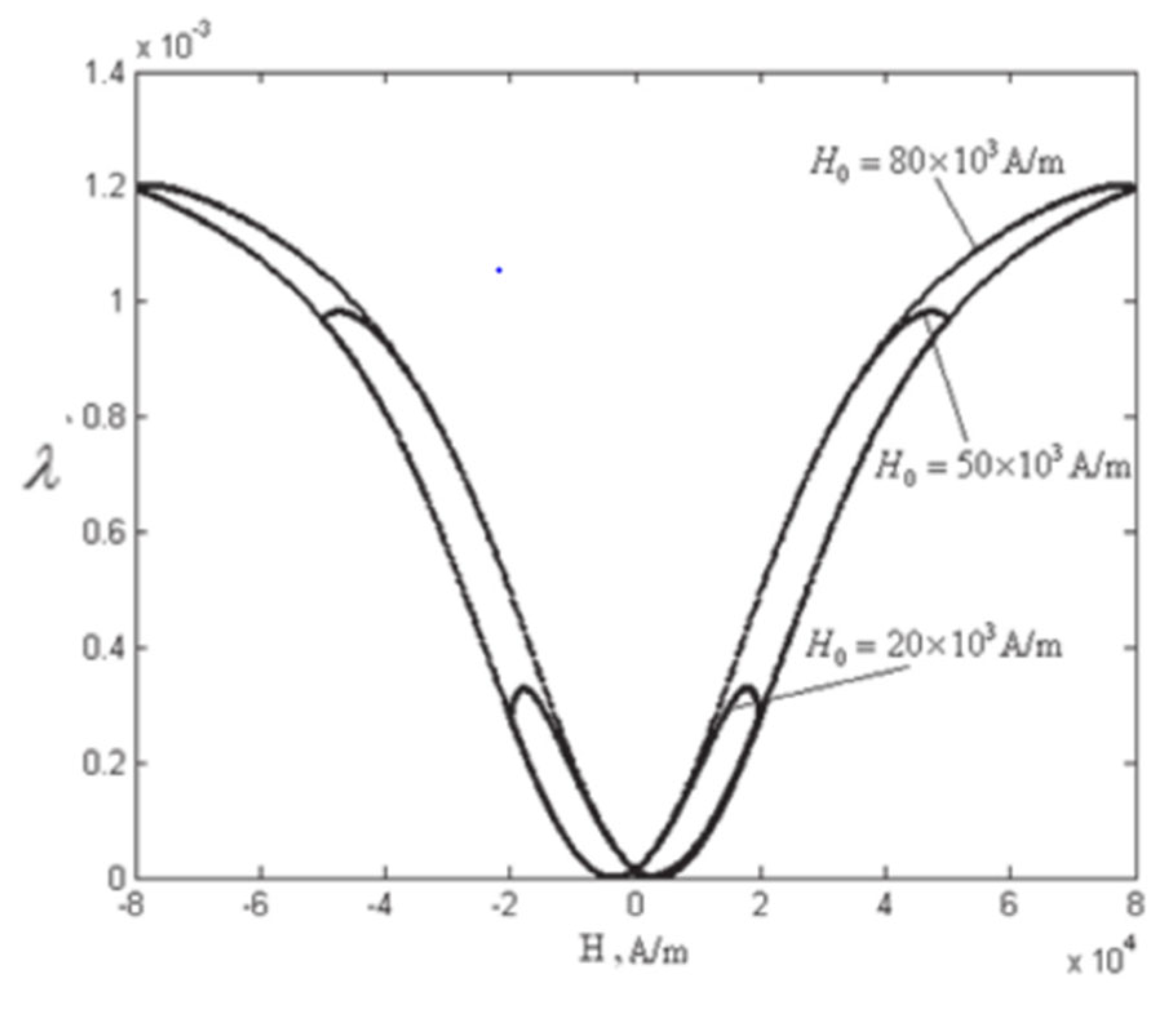
Figure 2. Prediction results and experimental data.

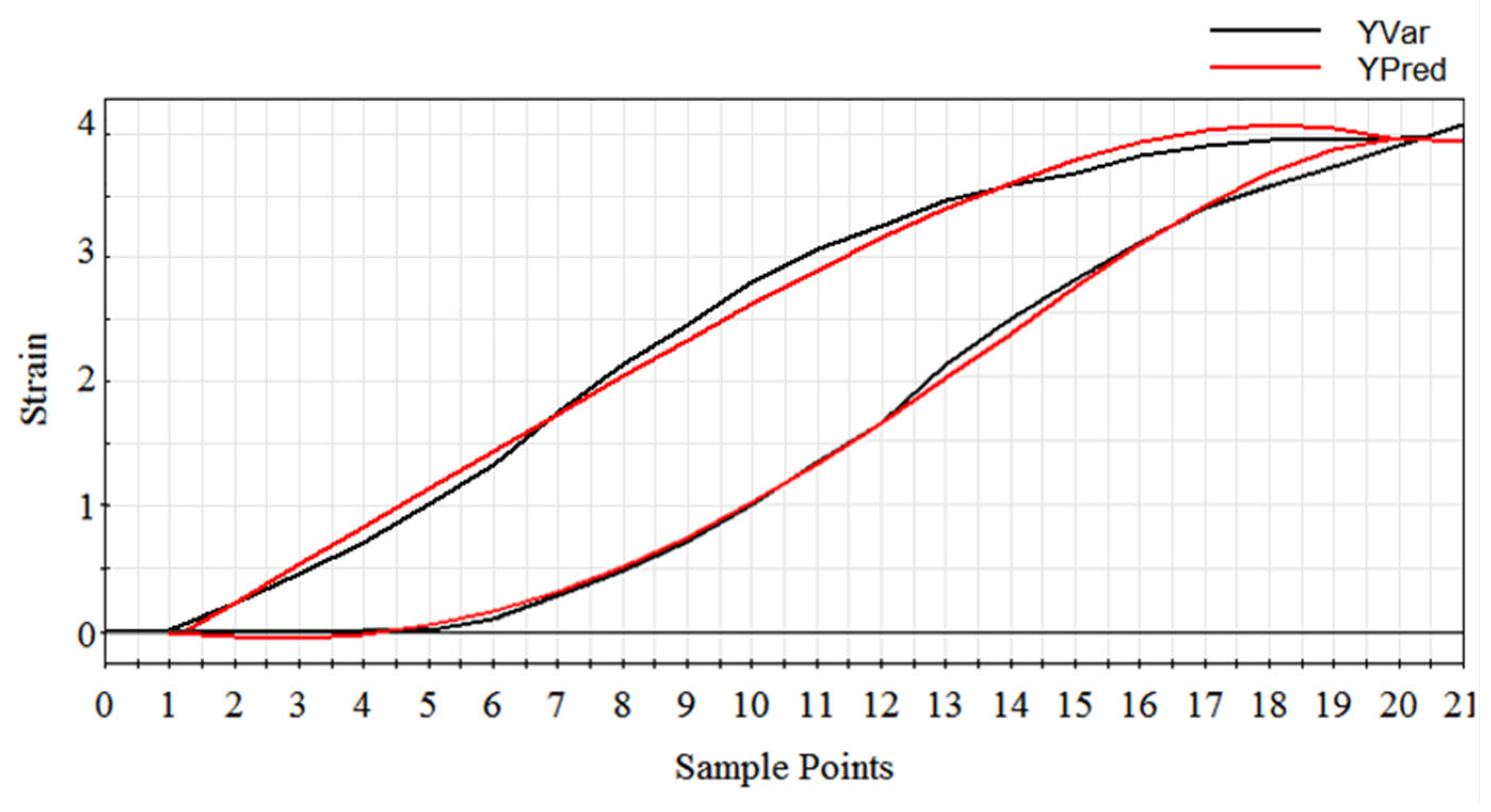
Figure 3. Phase diagram under different damping coefficients.

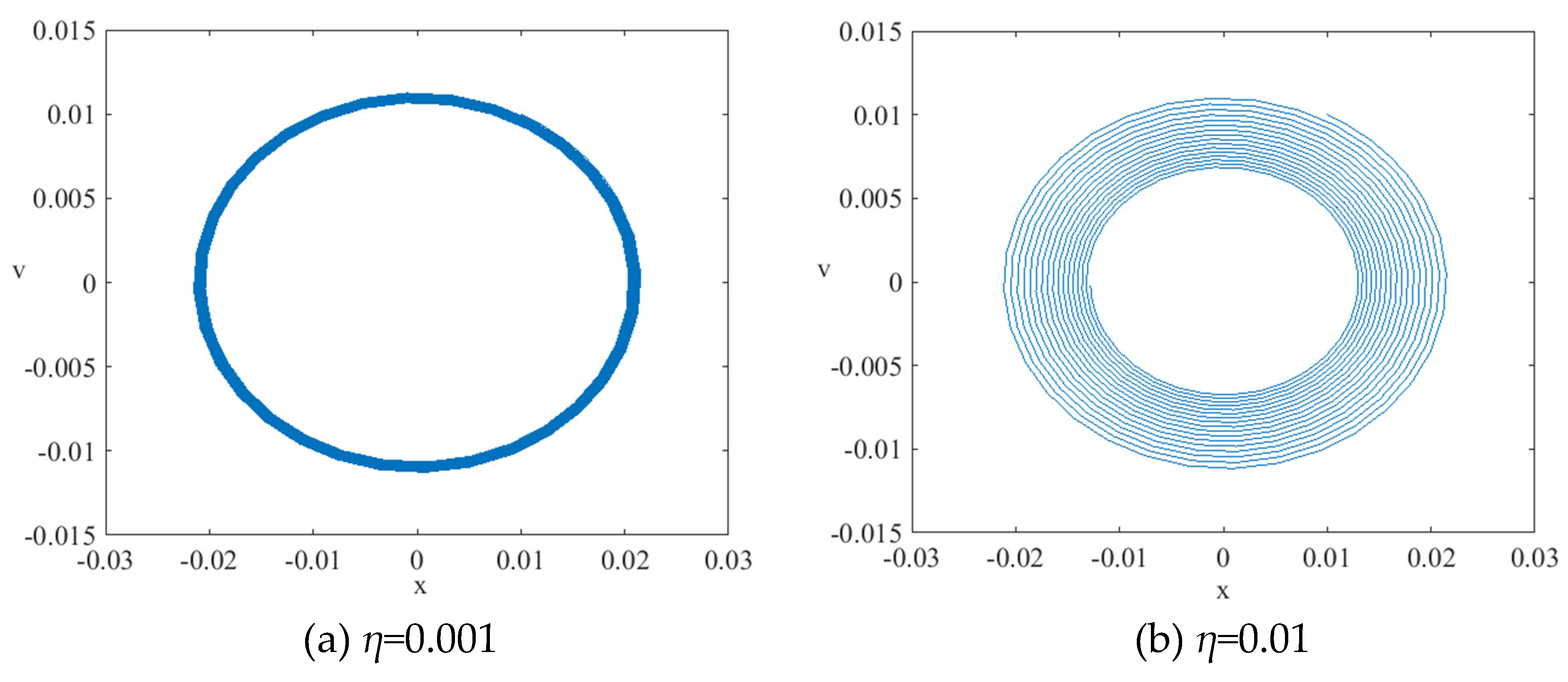
Figure 4. Phase diagrams under different excitation intensity and frequency.

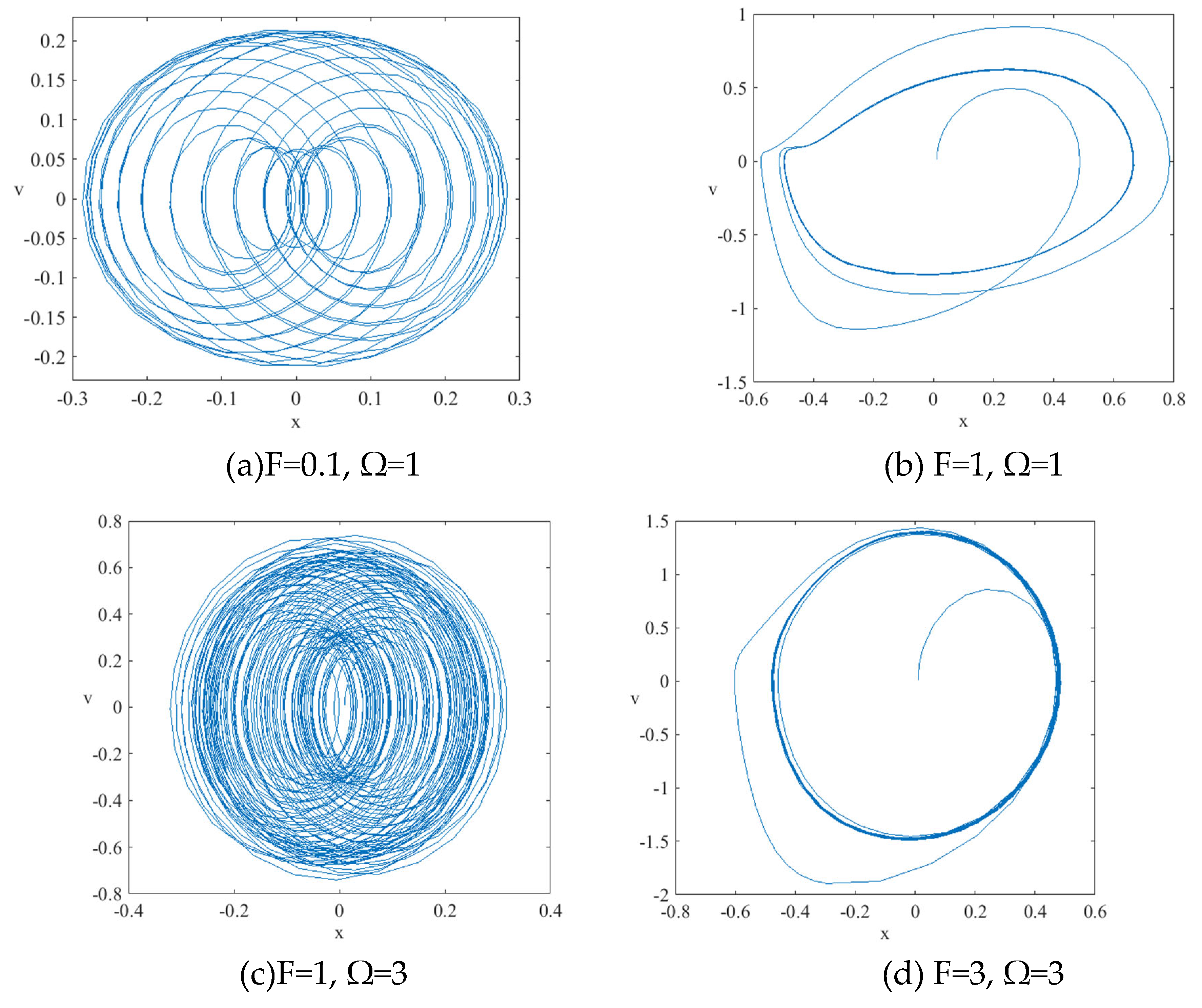
Figure 5. Joint probability density distribution diagram.

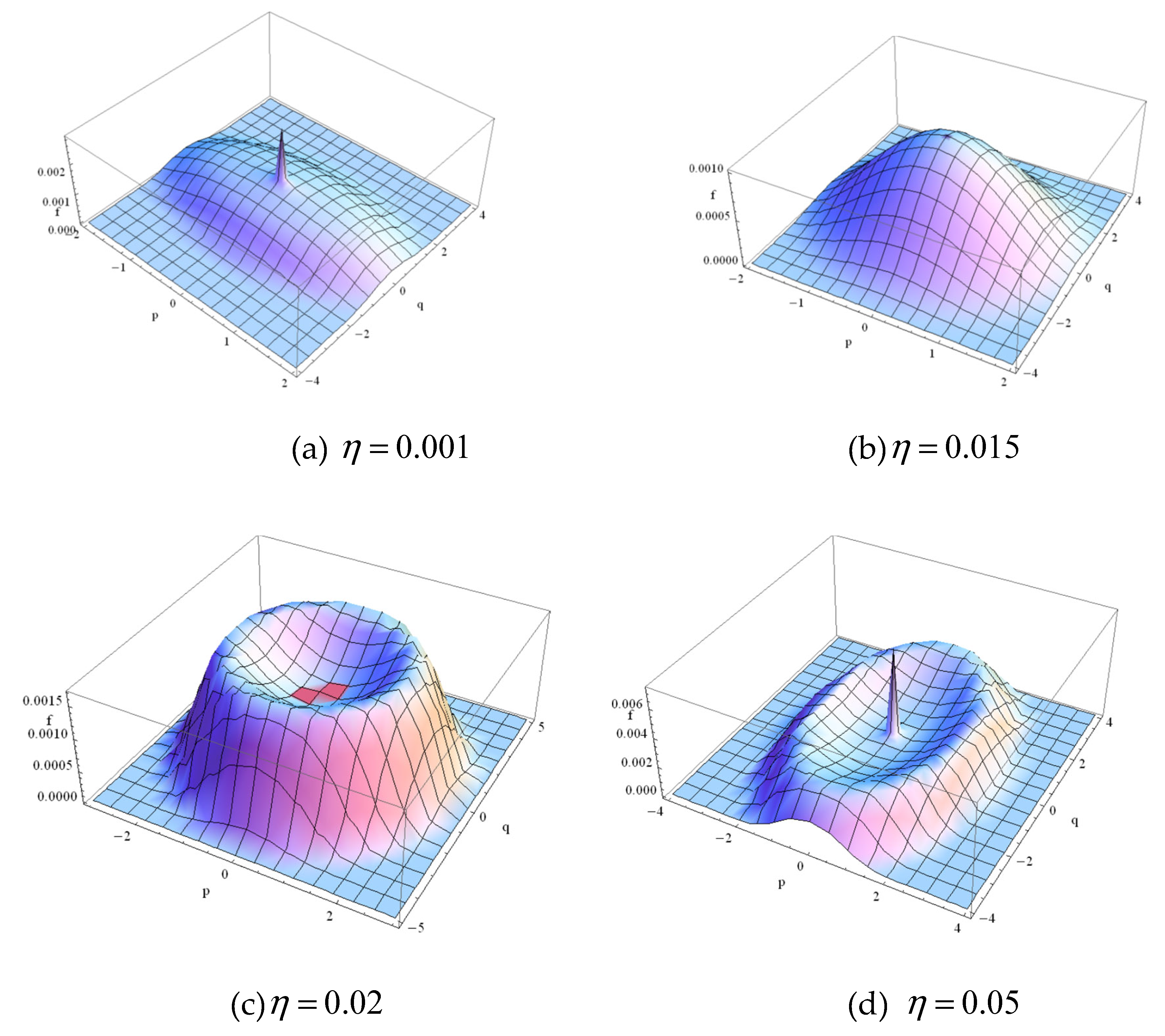
Figure 6. Schematic diagram of the structure of the fuzzy PID controller.

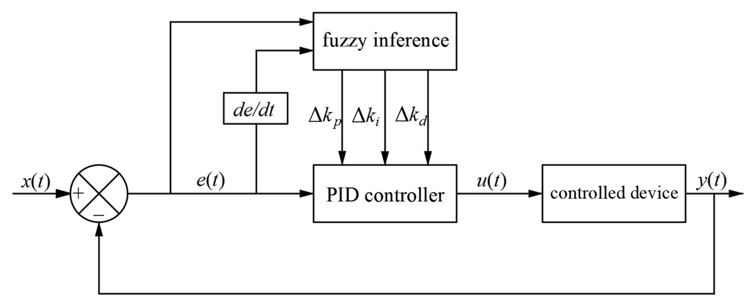
Figure 7. Membership function curve.

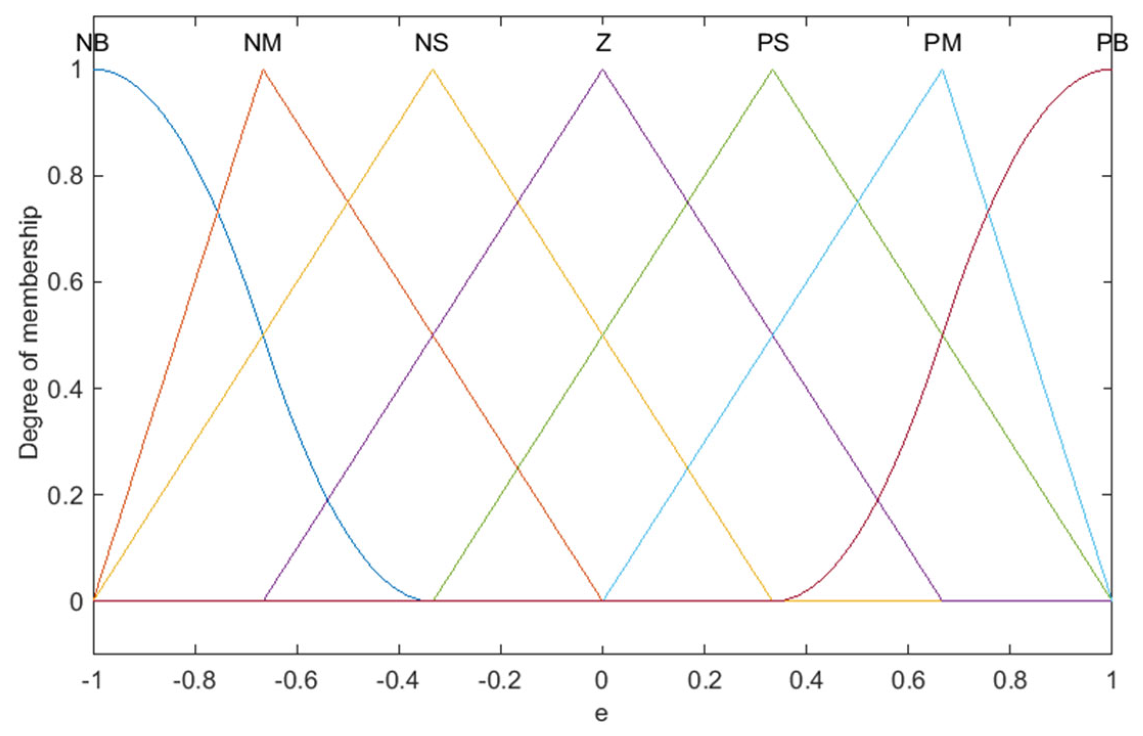
Figure 8. Δk_p, Δk_i, Δk_d Value graph.

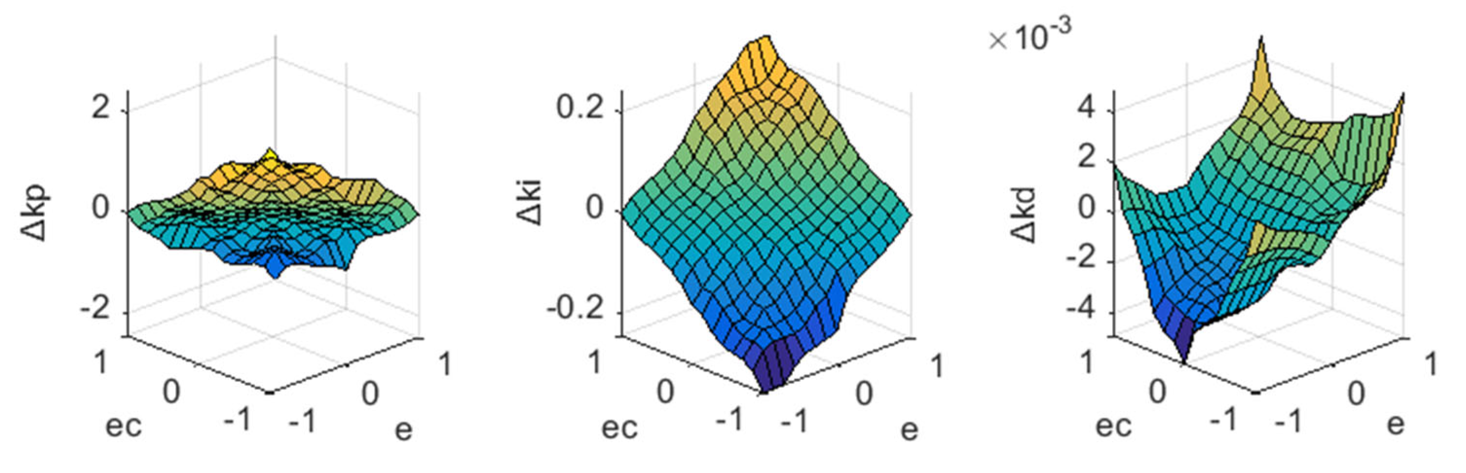
Figure 9. Simulation block diagram.

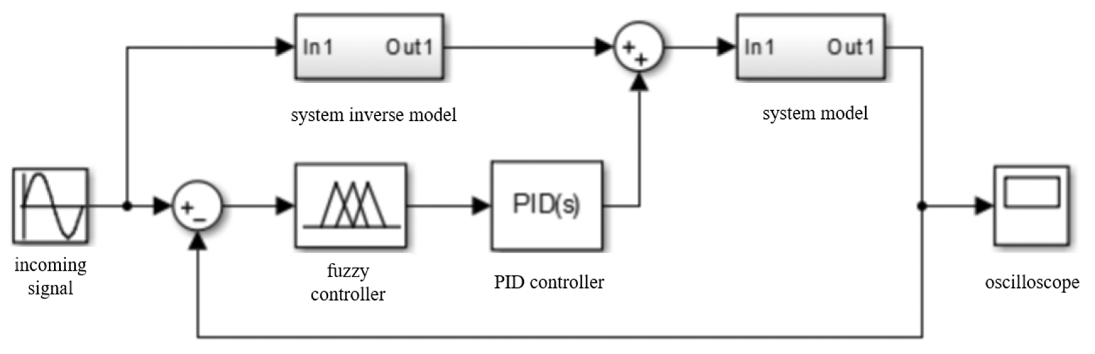
Figure 10. Feed-forward compensation fuzzy PID composite control displacement time curve.

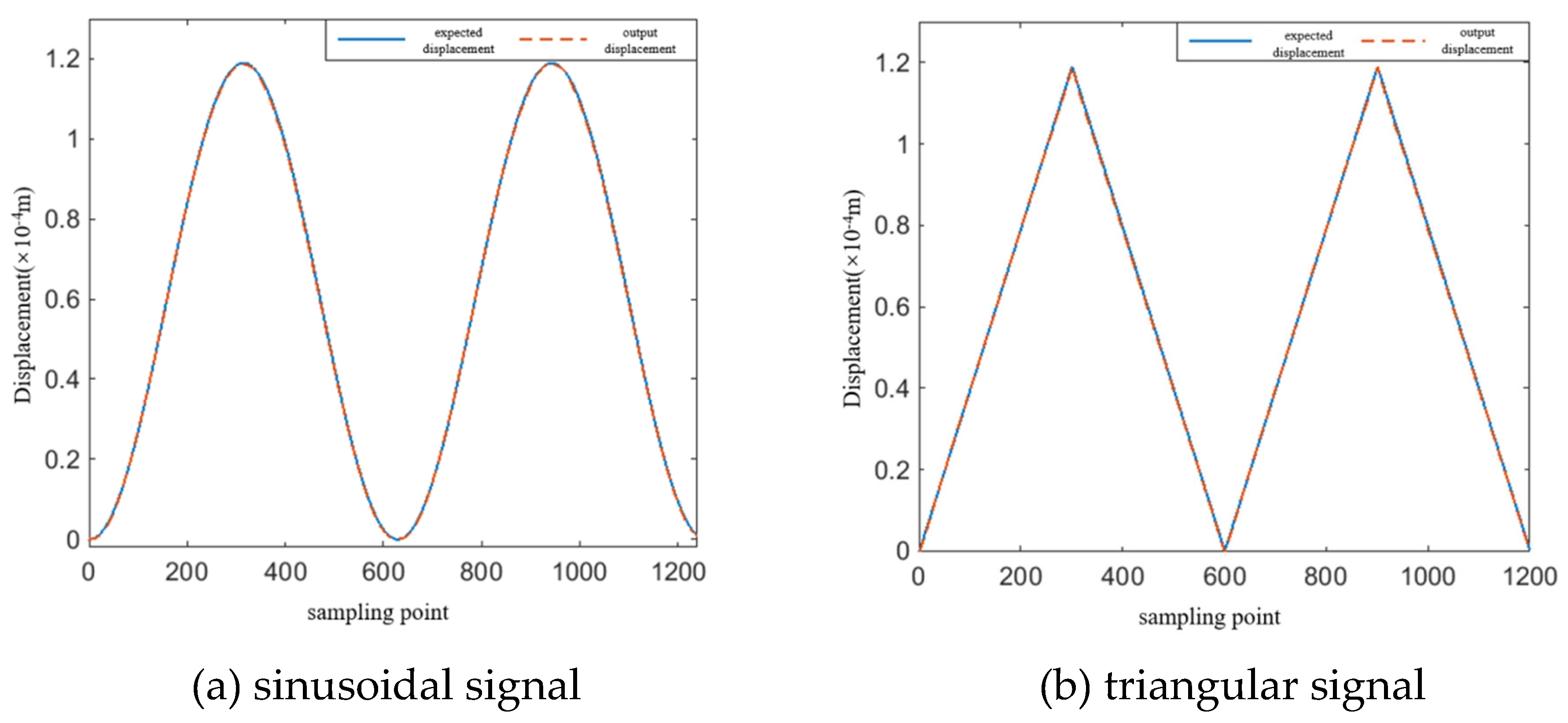
Figure 11. Sinusoidal signal displacement error.

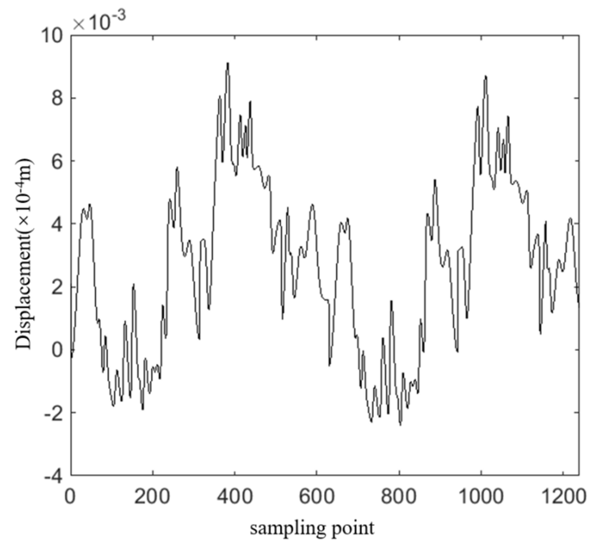
Table 1. Fuzzy rules.

Parameter	e	e_c
Parameter	e	NB	NM	NS	Z	PS	PM	PB
Δk_p	NB	PB	PB	PM	PM	PS	Z	Z
	NM	PB	PB	PM	PS	PS	Z	NS
	NS	PM	PM	PM	PS	PS	Z	NS
	Z	PM	PM	PS	Z	NS	NM	NM
	PS	PS	PS	Z	NS	NS	NM	NM
	PM	PS	Z	NS	NM	NM	NM	NB
	PB	Z	Z	NM	NM	NM	NB	NB
Δk_i	NB	NB	NB	NM	NM	NS	Z	Z
	NM	NB	NB	NM	NS	NS	Z	NS
	NS	NM	NM	NS	NS	Z	PS	PS
	Z	NM	NM	NS	Z	PS	PM	PM
	PS	NM	NS	Z	PS	PS	PM	PB
	PM	Z	Z	PS	PS	PM	PB	PB
	PB	Z	Z	PS	PM	PM	PB	PB
Δk_d,	NB	PS	NS	NB	NB	NB	NM	PS
	NM	PS	NS	NB	NM	NM	NS	Z
	NS	Z	NS	NM	NM	NS	NS	Z
	Z	Z	NS	NS	NS	NS	NS	Z
	PS	Z	Z	Z	Z	Z	Z	Z
	PM	PB	NS	PS	PS	PS	PS	PB
	PB	PB	PM	PM	PM	PS	PS	PB

Disclaimer/Publisher’s Note: The statements, opinions and data contained in all publications are solely those of the individual author(s) and contributor(s) and not of MDPI and/or the editor(s). MDPI and/or the editor(s) disclaim responsibility for any injury to people or property resulting from any ideas, methods, instructions or products referred to in the content.

© 2026 by the authors. Licensee MDPI, Basel, Switzerland. This article is an open access article distributed under the terms and conditions of the Creative Commons Attribution (CC BY) license (http://creativecommons.org/licenses/by/4.0/).

Copyright: This open access article is published under a Creative Commons CC BY 4.0 license, which permit the free download, distribution, and reuse, provided that the author and preprint are cited in any reuse.

Nonlinear Characteristics and Control Optimization of Giant Magneto Ultrasonic Transducers Under Random Excitation

Abstract

Keywords:

Subject:

Introduction

Establishment of the Constitutive Model of Giant Magnetostrictive Materials

Dynamic Analysis of Giant Magnetostrictive Ultrasonic Transducer

Dynamic Characteristics of Transducer under Stochastic Excitation

Control Scheme of Ultrasonic Transducer with GMUT

Conclusion

Acknowledgments

Conflicts of Interest

Appendix A

Appendix B

References

MDPI Initiatives

Important Links

Subscribe