

Submitted:
30 June 2026
Posted:
01 July 2026
You are already at the latest version
Abstract
This work addresses the simultaneous prediction of Marshall Stability (MS) and Indirect Tensile Strength (ITS) by integrating machine learning models with multi-objective optimization for the preliminary design of asphalt concrete. Based on 401 experimental samples, 15 variables were selected to describe asphalt properties, aggregate gradation, volumetric parameters, fiber characteristics, and production parameters, and four dual-output prediction models were developed. The models were evaluated through 20 Monte Carlo random splits. TabPFN and TabICLv2 showed better performance, with both models achieving a target-averaged RMSE of 0.94 and an R² of 0.87. Furthermore, Pareto filtering and TOPSIS ranking were combined to identify the top 10 non-dominated Pareto samples from valid samples, and the best overall solution was determined with MS = 15.23 kN and ITS = 3.90 MPa. The results indicate that mineral fibers are more suitable for improving balanced performance of MS and ITS, carbon fibers are more favorable for improving MS, and plastic fibers are more effective in improving ITS. Finally, a Streamlit-based graphical user interface was developed to enable real-time prediction and MS–ITS trade-off visualization, providing a reference for preliminary mix design of asphalt concrete.
Keywords:
asphalt concrete
; Marshall stability
; indirect tensile strength
; machine learning
; Pareto filtering
; TOPSIS ranking
1. Introduction
Asphalt concrete serves as a fundamental material in a wide range of civil infrastructure applications, particularly in highway pavements [1], airport surfaces [2], parking facilities [3], and impermeable core structures in embankment dams [4]. Its popularity stems from a combination of favorable engineering characteristics, such as adequate strength, water resistance, and economic efficiency throughout its service life [5,6,7]. However, the performance of asphalt concrete gradually changes when exposed to repeated loading, temperature fluctuations, oxidative aging, and other environmental influences [8,9,10]. These interacting factors can progressively deteriorate the mechanical performance of asphalt concrete and reduce the long-term reliability of engineering structures. Consequently, developing effective approaches for assessing and forecasting the mechanical behavior of asphalt concrete has become an essential task for material design, quality control, and infrastructure management.
Among the commonly used mechanical performance indicators, Marshall Stability (MS) and Indirect Tensile Strength (ITS) are two important parameters for evaluating asphalt concrete. MS is generally used to characterize the stability and deformation resistance of asphalt mixtures under loading [11], while ITS reflects the tensile resistance and cracking-related performance [12]. Two indicators describe different aspects of mechanical behavior and are not always improved simultaneously. A mixture with high MS may not necessarily exhibit excellent tensile resistance, and a mixture with high ITS may not always have the best stability or deformation resistance. Therefore, focusing only on a single performance indicator may lead to incomplete or biased mixture evaluation. Simultaneous consideration of MS and ITS is more suitable for assessing the balanced mechanical performance of asphalt concrete and supporting multi-objective mixture selection.
Traditional experimental methods provide direct and reliable measurements of asphalt mixture performance, but they are usually time-consuming, labor-intensive, and costly [13,14,15,16,17,18]. Changes in asphalt properties, aggregate gradation, volumetric parameters, fiber characteristics, and production-related conditions often require repeated laboratory tests to evaluate their effects on MS and ITS. In addition, the mechanical behavior of asphalt concrete is governed by complex nonlinear interactions among multiple variables, such as asphalt content, air voids, gradation structure, and fiber content. Empirical equations and simple statistical methods are usually limited by predefined assumptions and specific data ranges, making it difficult to accurately capture these interactive effects [19,20]. Moreover, traditional experimental or empirical approaches provide limited support for rapidly identifying mixtures with balanced MS and ITS performance from existing experimental data [21,22].
Machine learning provides a promising alternative for modeling the nonlinear relationship between mixture design variables and mechanical properties. In recent years, data-driven methods have been increasingly applied to predicting the properties of concrete materials, including compressive strength, tensile strength, elastic modulus, durability-related indicators, and other engineering performance parameters [23,24,25]. Traditional machine learning models, including Extreme Gradient Boosting (XGBoost) and Random Forest (RF), have also been widely employed in asphalt concrete research to predict key performance indicators such as Marshall stability, splitting strength, rutting resistance, and stiffness modulus [26,27].
Although previous studies have achieved encouraging results using machine learning techniques, the majority of adopted models are still based on conventional algorithms, such as neural-network models, bagging ensembles, and boosting ensembles. Their performance often depends on large dataset-specific training procedures and extensive hyperparameter tuning to achieve satisfactory predictive capability [28,29]. Recently, tabular foundation models, represented by Tabular Prior-data Fitted Network (TabPFN) and Tabular In-Context Learning version 2 (TabICLv2), have emerged as a new generation of machine learning methods for tabular data, showing promising potential in handling small-size, heterogeneous, and high-dimensional datasets with reduced tuning requirements [30,31]. In addition, existing studies have predominantly focused on predicting or optimizing a single performance indicator, whereas investigations that simultaneously consider multiple balanced mechanical properties, such as MS and ITS, are still limited.
To address the above issues, this study develops a machine learning framework for dual-parameter prediction of MS and ITS and data-driven mixture optimization for the preliminary design of asphalt concrete. The main innovations of this work are organized around the following three aspects. (1) A dual-parameter prediction framework for MS and ITS is established. By simultaneously considering deformation resistance and tensile resistance, this study provides a data-driven basis for comprehensive mechanical performance evaluation and multi-objective mixture selection of asphalt concrete. (2) Two emerging tabular foundation models, TabPFN and TabICLv2, are systematically compared with two optimized traditional tree-based ensemble models, RF and XGBoost, on a small-size, heterogeneous, and multi-variable asphalt concrete dataset, so as to evaluate the applicability of tabular foundation models to the MS–ITS dual-output prediction task. (3) An observed-data-driven mixture selection strategy is constructed by combining Pareto filtering and Technique for Order Preference by Similarity to Ideal Solution (TOPSIS) ranking in the MS–ITS objective space, through which the candidate mixtures with balanced stability and tensile resistance are identified from experimentally validated samples, providing reference guidance for mixture design. In addition, a Streamlit-based graphical user interface (GUI) is developed to integrate real-time prediction, MS–ITS performance trade-off visualization, and local interpretation, thereby improving the practical usability of the proposed framework for asphalt mixture analysis and preliminary design.
2. Materials and Methods
Figure 1 presents the general research framework of this study, which consists of four main stages: (1) An asphalt concrete database was constructed and preprocessed. The database contains 401 experimentally observed samples, with 15 input variables describing asphalt properties, aggregate gradation, volumetric parameters, fiber characteristics, and production-related information. MS and ITS were used as two output targets. (2) Dual-output machine learning models were developed to predict MS and ITS simultaneously. Two tabular foundation models, TabICLv2 and TabPFN, were compared with two traditional tree-based ensemble models, RF and XGBoost. For RF and XGBoost, Optuna was further used for hyperparameter tuning. (3) Model performance was evaluated through Monte Carlo cross-validation using multiple indicators, including RMSE, MAE, MAPE, MAD, and R². These metrics were further integrated into a composite score to support unified model comparison and ranking. (4) The experimentally observed mixtures were screened using Pareto filtering in the MS–ITS objective space, and the retained Pareto samples were ranked by TOPSIS. The selected models and trade-off analysis results were then integrated into a Streamlit-based GUI to support performance prediction, visualization, and preliminary mixture selection.
2.1. Dataset Preparation and Preprocessing
2.1.1. Data Collection and Variable Description
A dataset of 401 asphalt concrete mixtures was collected from 43 published studies covering the period 2003–2024, providing the basis for jointly modeling MS and ITS [32,33,34,35,36,37,38,39,40,41,42,43,44,45,46,47,48,49,50,51,52,53,54,55,56,57,58,59,60,61,62,63,64,65,66,67,68,69,70,71,72,73]. To represent the main mixture-design factors, 15 input variables were selected and grouped according to asphalt binder properties, aggregate gradation, volumetric indices, and fiber characteristics [26]. The asphalt-related features included penetration (Pe), ductility (Du), softening point (SP), and asphalt content (AC). The aggregate- and volumetric-related features included the passing percentages of 2.36 mm, 4.75 mm, and 9.5 mm aggregates (Ag2.36, Ag4.75, and Ag9.5), air voids (AV), voids in mineral aggregate (VMA), and voids filled with asphalt (VFA). The fiber- and production-related features included fiber type (FT), fiber content (FC), fiber length (FL), tensile strength (TS), and mixing temperature (MT). In contrast to previous single-output studies that focused on only one mechanical property, both MS and ITS were used as output variables in this study to support multi-target performance prediction and subsequent multi-objective mixture design optimization.
For the categorical feature FT, the original fiber names were standardized into seven representative groups, including plastic fiber, mineral fiber, bio-fiber, carbon fiber, glass fiber, steel fiber, and no fiber. Among the 401 samples, 249 samples contained fiber reinforcement, whereas 152 samples were non-fiber asphalt concrete mixtures. The distribution of fiber categories is shown in Table 1.
2.1.2. Data Analysis
Table 2 reports the descriptive statistics for all input and output variables, including extreme values, quartiles, means, and standard deviations. Overall, the dataset spans broad ranges of binder properties, gradation indices, volumetric parameters, fiber descriptors, and production conditions, reflecting the diversity of the collected experimental sources. For asphalt-related variables, penetration, ductility, softening point, and asphalt content all show varying degrees of variation, reflecting differences in asphalt materials and mixture design. The aggregate gradation variables Ag2.36, Ag4.75, and Ag9.5 also have wide value ranges, indicating that the database contains asphalt mixtures with different gradation structures. The fiber-related variables also show obvious dispersion, especially fiber length, fiber tensile strength, and fiber content, because the database includes both fiber-reinforced asphalt concrete and non-fiber asphalt concrete samples. Among the two output variables, MS ranges from 3.40 to 26.72 kN, while ITS ranges from 0.20 to 3.94 MPa, indicating that the database covers asphalt concrete samples with different levels of mechanical performance.
Figure 2 gives the Pearson correlation matrix for the input descriptors and target responses. It can be observed that high correlation coefficients mainly appear between variables with clear physical relationships. For example, different sieve passing indicators, including Ag2.36, Ag4.75, and Ag9.5, show strong positive correlations, because these variables jointly characterize the gradation composition of the mixture. Meanwhile, relatively strong correlations are also observed among volumetric parameters such as AV, VMA, and VFA, which is consistent with their inherent relationships in definition and calculation. After excluding these expected physical associations, the remaining feature pairs all have absolute Pearson coefficients below 0.7 [24], suggesting that severe multicollinearity is not present. Thus, the selected variables provide complementary descriptions of mixture composition and mechanical behavior and were retained as inputs for subsequent machine learning analysis.
2.1.3. Data Preprocessing
Before model training, the constructed database was preprocessed to ensure data format consistency and meet the input requirements of machine learning models [74]. For fiber-related variables, it was necessary to distinguish between “non-fiber samples” and “missing data”. For non-fiber asphalt concrete samples, FC, FL, and TS were all assigned values of 0 to indicate the absence of fiber reinforcement in these samples. Meanwhile, the categorical variable FT was unified into seven representative categories, including plastic fiber, mineral fiber, bio-fiber, carbon fiber, glass fiber, steel fiber, and no fiber. The final dataset consisted of 15 input variables and 2 output variables. To evaluate the predictive capability of the models on unknown samples, the database was divided into training and testing sets at a ratio of 8:2 in each Monte Carlo random split, where 80% of the samples were used for model training and 20% were used for model testing. This random splitting process was repeated 20 times to reduce the influence of a single data partition on the model evaluation results.
2.2. Machine Learning Models
Table 3 lists the four models evaluated in this work: two tabular foundation models and two conventional tree-based ensemble models. Specifically, TabICLv2 and TabPFN belong to tabular foundation models, while RF and XGBoost represent typical ensemble learning models based on Bagging and Boosting strategies, respectively. The purpose of selecting these four types of models is to compare the prediction ability of emerging tabular foundation models and traditional machine learning models on a small-scale, multi-variable, and dual-output asphalt concrete dataset.
Figure 3 further illustrates the basic differences between traditional machine learning models and tabular foundation models. Conventional models are generally fitted directly on the task-specific dataset and learn relationships between mixture descriptors and target properties from those samples. For example, RF improves stability by aggregating the outputs of multiple decision trees [75], while XGBoost continuously corrects the prediction errors of the previous model through a stepwise boosting strategy [76], thereby improving model fitting ability and generalization performance. These models have relatively good interpretability and a mature application basis, and are therefore suitable as traditional benchmark models in this study. Different from traditional models, TabPFN and TabICLv2 are recently developed tabular foundation models, whose core advantage lies in using pretraining or in-context learning mechanisms to handle tabular prediction tasks. TabPFN acquires general-purpose tabular modeling ability from extensive pretraining on synthetic tasks and uses contextual information to generate predictions for new small-sample regression tasks [30]. TabICLv2 is also based on the idea of pretrained tabular models, and can extract potential relationships among variables from limited samples and directly apply them to the current prediction task [31]. Therefore, these models have potential advantages in material property prediction problems with limited sample sizes and complex variable types.
2.3. Evaluation Metrics and Monte Carlo Validation
The prediction task in this study contains two response variables with different physical meanings and numerical scales: MS and ITS. For this reason, prediction errors were not pooled across the two outputs. Instead, each metric was first computed for MS and ITS separately within each Monte Carlo split, and the two target-specific values were then averaged to obtain a target-averaged summary for model comparison.
Let s denote the index of a Monte Carlo split, k denotes the target variable, where k belongs to {MS, ITS}, and i denote the sample index in the corresponding training or testing subset. For split s, the notation in Eq. (1) represents the measured value, predicted value, and residual of target k for sample i. The residual was defined as follows:
where is the Monte Carlo split index; identifies the predicted target; is the sample index; and , , and denote the measured value, predicted value, and residual of target for sample in split , respectively.
Based on the target-specific residuals, five indicators were calculated for each target. The root mean square error (RMSE) and mean absolute error (MAE) quantify the magnitude of prediction errors in the original unit of the target variable, whereas the mean absolute percentage error (MAPE) expresses the relative error as a percentage. The coefficient of determination (R²) measures the explained variance, and the median absolute deviation (MAD) was calculated from the residuals around their median to provide a robust description of residual dispersion.
In Eqs. (2)-(6), denotes the number of samples in the evaluated subset of split ; is the mean measured value of target in that subset; and and indicate median operations over the corresponding sample indices. Smaller RMSE, MAPE, MAE, and MAD values correspond to lower prediction errors, while a larger indicates stronger agreement between measured and predicted values.
For a generic metric M, the split-wise multi-target value was obtained by averaging the MS and ITS results. This target-averaged calculation keeps the two response variables equally represented while avoiding direct residual aggregation across variables with different units.
To reduce sensitivity to a particular random data partition, the complete training and testing procedure was repeated over S = 20 Monte Carlo splits. The reported value of each target-averaged metric was the mean across all splits, and the corresponding standard deviation was used to describe split-to-split variability.
In Eqs. (7)-(9), represents any one of the five evaluation metrics; is the target-averaged metric value in split ; is the total number of Monte Carlo splits; is the split-averaged value; and is the corresponding split-to-split standard deviation retained in the final performance table.
2.4. Model Ranking and Comprehensive Evaluation
The five metrics describe complementary aspects of model behavior and do not share the same optimization direction. Therefore, the original test-set metrics were converted into direction-consistent and dimensionless utility scores before calculating an overall ranking. This procedure was applied only to the testing results so that the final comparison reflected generalization performance rather than training-set fit.
For each model and metric, the raw test metric was first averaged across the two targets, as shown in Eq. (10). The target-specific terms in the equation correspond to the MS and ITS values of the same metric.
The target-averaged values were then transformed into utility values with a common direction. Because smaller values are preferred for RMSE, MAPE, MAE, and MAD, these four metrics were multiplied by -1. In contrast, R² was kept unchanged because a larger value represents better predictive performance.
For each metric, the utility values were standardized across all candidate models. The mean and standard deviation used in this transformation are denoted in Eq. (12), and the standardized score was calculated as follows:
The standardized values were further mapped to a bounded interval using a sigmoid transformation. This step makes the scores easier to compare and reduces the influence of unusually large standardized differences on the final ranking. The scaling parameter was set to α = 0.5, consistent with the implemented scoring workflow.
The final composite score for each model was obtained by averaging the five normalized metric scores. All five metrics were given equal weight to prevent the ranking from being controlled by a single error or goodness-of-fit measure.
In Eqs. (10)-(14), denotes the candidate model and denotes the evaluation metric; and are the target-specific test metrics; is the target-averaged raw metric; is the direction-consistent utility value; and are the across-model mean and standard deviation for metric ; is the standardized utility; is the sigmoid-normalized score; is the sigmoid scaling parameter; and is the final comprehensive score used for model ranking.
A larger composite score indicates a better overall balance among prediction accuracy, relative error, explained variance, and residual robustness. The same direction-unification and normalization principle was also used to support radar-chart visualization of the five-dimensional testing performance.
2.5. Hyperparameter Tuning Through Optuna
To improve the predictive performance of traditional tree-based ensemble models, Optuna was used in this study to automatically optimize the key hyperparameters of RF and XGBoost [77]. In contrast, TabICLv2 and TabPFN are tabular foundation models whose predictive ability is mainly derived from pretraining or in-context learning. Therefore, their default configurations were adopted in this study, and no additional hyperparameter search was performed for them.
Figure 4 shows the Optuna-based hyperparameter tuning workflow. First, the corresponding hyperparameter search spaces were defined according to the characteristics of RF and XGBoost. Then, in each trial, Optuna automatically generated a candidate set of hyperparameters and constructed the corresponding model on the training set. After model training, the objective function values were calculated through 5-fold cross-validation within the training set, where the cross-validation process was randomly shuffled and the random seed was set to 42. For each model to be optimized, Optuna performed 500 trials to search for a better hyperparameter combination within the predefined search space. Since this study simultaneously predicted two mechanical performance indicators, MS and ITS, a multi-objective optimization strategy was adopted. Specifically, the cross-validation RMSE values of MS and ITS were used as two independent optimization objectives, and both were minimized simultaneously through the multi-objective optimization mechanism of Optuna. After optimization, the compromise solution with the smallest normalized average error was selected from the Pareto-optimal solution set as the final hyperparameter combination. After the hyperparameter search was completed, the selected hyperparameter combination was used for subsequent model training and testing evaluation. Through this tuning process, the predictive stability and generalization capability of traditional tree-based ensemble models in the MS–ITS dual-output prediction task can be improved while maintaining a fair model comparison.
2.6. Pareto Filtering and TOPSIS-Based Selection of Observed Experimental Mixtures
To support multi-objective mixture selection using only experimentally observed data, the cleaned database was first filtered to retain samples with valid MS and ITS values. Both MS and ITS were treated as benefit criteria because larger values indicate better mechanical performance. As shown in Figure 5, the observed-data selection workflow consisted of three main steps: valid-sample filtering, Pareto-based non-dominated mixture identification, and TOPSIS-based ranking of the retained Pareto samples.
Specifically, non-dominated observed mixtures were identified by Pareto filtering in the two-dimensional MS–ITS objective space [78]. A mixture was retained as a true-data Pareto sample when no other observed mixture simultaneously achieved equal-or-higher MS and ITS with at least one strictly higher objective value. The retained Pareto candidates were subsequently prioritized with TOPSIS [79,80]. The equal-weight scenario, in which MS and ITS were assigned weights of 0.5 and 0.5, respectively, was used as the primary ranking scheme.
3. Results and Discussion
3.1. Hyperparameter Optimization Results
Figure 6 shows the optimization histories of RF and XGBoost during Optuna tuning. In this study, the cross-validation RMSE values of MS and ITS were used as two independent optimization objectives, and the compromise solution with the smallest normalized average error was selected from the Pareto-optimal solution set as the final hyperparameter combination. From the optimization process, the objective function values of both RF and XGBoost decreased noticeably in the early trials, indicating that Optuna could gradually eliminate poorly performing parameter combinations within the predefined search space and locate parameter regions more suitable for the MS–ITS dual-output prediction task. As the number of trials increased, the further improvement in the best cross-validation error gradually became smaller, and the optimization curves generally tended to stabilize, suggesting that 500 trials were basically sufficient for the hyperparameter search of the traditional tree-based models in this study. It should be noted that, because MS and ITS were optimized simultaneously, the final selected parameter combination did not simply pursue the lowest error for a single objective, but reflected a compromise optimization result between the two mechanical performance indicators.
According to the optimization results, RF finally adopted a relatively large number of trees and a deep tree structure to enhance its ability to fit nonlinear relationships among variables. XGBoost adopted a relatively large number of weak learners, a shallow tree depth, and moderate regularization parameters to balance model complexity and generalization capability. The specific hyperparameter settings are shown in Table 4. Based on the optimized parameter combinations, RF and XGBoost were further included in the unified Monte Carlo testing evaluation together with TabICLv2 and TabPFN, so as to compare the generalization performance of traditional tree-based ensemble models and tabular foundation models in the MS and ITS dual-output prediction task.
3.2. Prediction Performance
Figure 7 shows the comparison between measured and predicted values of the four models in the MS and ITS prediction tasks. Overall, most prediction points of TabICLv2, TabPFN, RF, and XGBoost are distributed near the 1:1 reference line, indicating that all four models can reasonably capture the nonlinear relationships between the input variables and the two mechanical properties. Among them, the prediction points of TabPFN and TabICLv2 are generally closer to the reference line. Both models achieved an average RMSE of 0.94 and an R² of 0.87, showing good fitting consistency and prediction accuracy. In comparison, RF and XGBoost can also reflect the overall variation trends of MS and ITS, but their prediction points are relatively more scattered for some high-performance or low-performance samples, with RMSE values of 1.00 and 1.01 and R² values of 0.85 and 0.84, respectively. These results indicate that the traditional tree-based ensemble models after Optuna tuning still have strong predictive capability, while TabICLv2 and TabPFN show better overall generalization performance in the small-scale, multi-variable, and dual-output prediction scenario of this study.
To uniformly compare the predictive performance of different models, Figure 8 presents the comprehensive evaluation results based on five metrics: RMSE, MAE, MAPE, MAD, and R². Specifically, Figure 8(a) shows the normalized metric scores after direction unification and standardization, while Figure 8(b) presents the composite scores used for overall model ranking. The detailed test-set performance statistics are provided in Appendix A, Table A2. Since these metrics reflect different aspects of model performance, including prediction error, relative error, explanatory ability, and residual robustness, and their optimization directions are not fully consistent, the original metric values were first converted into direction-consistent and dimensionless scores before calculating the composite score. This procedure helped avoid model ranking being dominated by a single metric. The results show that TabPFN and TabICLv2 achieved similar comprehensive performance, although their advantages were slightly different. TabPFN obtained the lowest MAPE of 9.98%, indicating a slight advantage in controlling relative prediction error, whereas TabICLv2 achieved the lowest MAD of 0.40, suggesting a more stable residual distribution. In comparison, RF and XGBoost performed slightly worse than the two tabular foundation models across the comprehensive evaluation metrics, but they still maintained acceptable prediction accuracy and can therefore serve as reliable benchmark models.
3.3. Observed-Data Pareto Front and TOPSIS-Based Mixture Selection
3.3.1. Observed Pareto Front and TOPSIS Ranking
The observed-data selection results are summarized in Figure 9. After filtering the experimental database, 401 samples with valid MS and ITS values were retained for multi-objective evaluation, among which only 10 samples were identified as true-data Pareto samples. These samples represent the experimentally observed upper boundary of the MS-ITS objective space, where no other observed mixture simultaneously achieved equal-or-higher MS and ITS with at least one strictly higher objective value.
As shown in Figure 9, most observed mixtures were concentrated in the moderate-performance region, whereas the Pareto samples formed the upper-right boundary of the objective space. The MS-best observed sample, E275, achieved the highest MS value of 26.72 kN but had a relatively lower ITS of 1.66 MPa. In contrast, the ITS-best observed samples, E041 and E251, reached an ITS of 3.94 MPa but showed a lower MS value of 10.78 kN. This contrast confirms that optimizing a single mechanical indicator may bias mixture selection away from balanced performance.
Within the Pareto set, the equal-weight TOPSIS ranking selected E134 as the observed-data compromise mixture, with MS = 15.23 kN, ITS = 3.90 MPa, and a Pareto-set TOPSIS score of 0.55. This mixture was not the single-objective maximum for either MS or ITS, but it was closest to the equal-weight ideal solution because it combined a high ITS level with a moderate-to-high MS level.
3.3.2. Design Implications for Mixture Selection
Based on the full set of ten observed-data Pareto solutions, the key shared features of different design pathways are summarized in Table 5. The complete feature-level information for all Pareto solutions is provided in Appendix A, Table A3, so that the design-oriented summary in the main text remains concise while the full data remain traceable.
The grouped Pareto solutions provide several design-oriented implications. For balanced MS–ITS performance, E134 and E124 suggest that mineral fiber or basalt fiber systems can be regarded as a reasonable candidate window. These samples correspond to a relatively low fiber content of 0.20%–0.30%, a fiber length of 6 mm, and an asphalt content of 5.27%–5.80%, resulting in MS values of 13.06–15.23 kN and high ITS values of 3.90–3.91 MPa. This indicates that a low-dosage and short-length mineral-fiber system may be more favorable for simultaneously maintaining stability and tensile strength.
For MS-dominant design, the carbon-fiber Pareto solutions, including E275, E277, E278, and E279, showed much higher MS values of 19.22–26.72 kN. These mixtures were mainly associated with a fiber content of 0.40%–0.80%, a fiber length of 6 mm, and an asphalt content of 5.90%–6.70%. However, their ITS values were only 1.66–2.06 MPa, indicating that carbon fiber is more suitable for stability-oriented improvement, while tensile performance may still require compensation through other mixture-design parameters.
For ITS-dominant design, the plastic-fiber samples E041 and E251 achieved the highest ITS value of 3.94 MPa, with a fiber content of approximately 0.23% and an asphalt content of 3.80%–4.00%. However, their MS value was only 10.78 kN, suggesting that this pathway is more suitable for tensile-strength-oriented improvement and that additional optimization of asphalt content, gradation, or volumetric parameters may be needed to improve stability. In addition, the no-fiber sample E081 also entered the Pareto front, showing that fiber reinforcement is not the only route to obtaining a favorable MS–ITS combination. Overall, the observed-data Pareto solutions should be interpreted as design guidance within the current database, and mixture selection should be made according to whether the target is balanced performance, MS-dominant performance, or ITS-dominant performance.
4. Graphical User Interface Platform
To improve the practical applicability of the established model in predicting the performance of asphalt mixtures, a web-based graphical user interface platform was developed using Streamlit. The platform is available at https://acmsitsgui-35achzf3lbbswu8cjarmmj.streamlit.app/, as shown in Figure 10. It integrates real-time MS and ITS prediction and performance trade-off visualization. After users input mixture composition, gradation parameters, volumetric parameters, and fiber-related variables, the platform outputs predicted MS and ITS values and marks current prediction point in the MS-ITS performance trade-off plot, allowing users to intuitively evaluate its position relative to experimental samples and the Pareto front. In addition, an optional SHAP-based local explanation module is embedded in the platform to help users inspect feature contributions for a given prediction [81].
5. Discussion
5.1. Overall Effectiveness
The machine learning framework constructed in this study shows good overall effectiveness in the dual-index prediction of MS and ITS and mixture selection for asphalt concrete. First, the database established based on 401 experimental samples covers multiple types of influencing factors, including asphalt properties, aggregate gradation, volumetric parameters, fiber characteristics, and production parameters, providing a relatively complete data basis for the simultaneous prediction of Marshall stability and indirect tensile strength. Second, TabPFN and TabICLv2 show good generalization ability in small-sample, multi-variable, and highly heterogeneous tabular data scenarios, and their comprehensive predictive performance is slightly better than that of traditional tree-based ensemble models, indicating that tabular foundation models have certain application potential in the prediction of mechanical properties of asphalt mixtures. At the same time, RF and XGBoost optimized by Optuna still maintain high prediction accuracy and stability, suggesting that traditional machine learning models can still serve as reliable benchmark methods for similar material property prediction tasks. On this basis, the mixture selection method based on observed-data Pareto filtering and TOPSIS can identify candidate schemes with a good balance between MS and ITS from existing experimental samples, avoiding the neglect of performance trade-offs caused by focusing only on a single mechanical indicator. Finally, the developed Streamlit graphical user interface further integrates dual-target performance prediction and MS–ITS trade-off visualization, enabling the model results to serve asphalt mixture proportion analysis and preliminary design decisions in a more intuitive manner.
5.2. Challenges and Limitations
Although the machine learning framework constructed in this study shows good effectiveness in the dual-index prediction of MS and ITS and mixture selection, some challenges and limitations still remain. (1) The current database contains 401 experimental samples, and the data scale is relatively limited, with a certain degree of heterogeneity in sample sources. Material sources, test conditions, and preparation processes may differ among different studies. Meanwhile, some important material parameters and test information have not yet been included as model inputs, such as fiber surface treatment methods, aggregate morphology, asphalt modification type, and forming method. This may limit the model’s ability to fully characterize complex material behavior. (2) For non-fiber asphalt concrete samples, this study assigned fiber-related variables such as fiber content, fiber length, and tensile strength to 0 to distinguish non-fiber samples from fiber-reinforced samples. Although this treatment helps unify the data format and meet the input requirements of the models, it may also introduce certain encoding correlations among fiber-related variables, thereby affecting the model’s independent identification of fiber effects. (3) The Pareto filtering and TOPSIS methods adopted in this study mainly conduct performance trade-off analysis and candidate mixture selection within the range of existing experimental samples. Therefore, the results should be understood as balanced selections within the current database rather than globally optimal mix proportions. In addition, this study only used Marshall stability and indirect tensile strength as optimization objectives, and has not further considered factors such as moisture stability, fatigue performance, material cost, and environmental impact. Therefore, the current selection results are more suitable as references for preliminary mix proportion analysis and subsequent experimental validation, rather than directly replacing a complete engineering design and performance evaluation process.
5.3. Future Research Perspectives
In response to the above limitations, future research can further improve the current framework from three aspects: data expansion, variable encoding optimization, and multi-objective design extension. First, the scale of the asphalt concrete database should be continuously expanded, and the completeness and consistency of data fields should be improved. In addition to the existing asphalt properties, gradation, volumetric parameters, and fiber characteristics, future studies can further include information such as fiber surface treatment methods, aggregate morphology, asphalt modification type, forming method, test temperature, and loading conditions. This would allow the effects of different material compositions and test conditions on MS and ITS to be more comprehensively characterized, and improve the generalization ability of the model on external data and in practical engineering scenarios. Second, regarding the differences between non-fiber samples and fiber-reinforced samples, future studies can explore more reasonable feature representation methods, such as introducing an independent fiber-presence variable, adopting group-based modeling strategies, or designing encoding methods more suitable for mixed-type material data. These methods may reduce the encoding correlations caused by zero assignment of fiber-related variables and enhance the model’s ability to independently identify fiber effects. Finally, in terms of mixture selection and optimization, future studies can further combine machine learning prediction models, engineering constraints, and multi-objective optimization algorithms on the basis of the existing observed-data Pareto filtering and TOPSIS analysis, so as to generate and screen new candidate mix proportions. Meanwhile, the optimization objectives should also be extended from MS and ITS to multiple dimensions, including moisture stability, fatigue performance, material cost, and environmental impact. The reliability of the model-recommended results should also be verified through experiments, thereby promoting the development of the current framework from preliminary performance analysis toward a more complete intelligent design method for asphalt mixtures.
6. Conclusions
This study constructed a machine learning framework for the dual-parameter prediction of Marshall stability and indirect tensile strength and data-driven mixture optimization for the preliminary design of asphalt concrete. Based on the current research results, the main conclusions are as follows:
- This study established an asphalt concrete database containing 401 experimental samples, and selected 15 input variables to characterize factors, such as asphalt properties, aggregate gradation, volumetric parameters, fiber characteristics, and production parameters. Different from prediction tasks that focus only on a single mechanical property, this study used both MS and ITS as output indicators, providing a data basis for the dual-index performance prediction and subsequent mix proportion selection of asphalt mixtures.
- In terms of model prediction, TabPFN and TabICLv2 showed good comprehensive predictive ability in small-sample and multi-variable tabular data scenarios, and their overall performance was slightly better than that of RF and XGBoost optimized by Optuna. For MS prediction, the test-set R² values of both TabPFN and TabICLv2 exceeded 0.90, with an average RMSE of approximately 1.0–1.2 kN. For ITS prediction, the test-set R² values of the two models remained above 0.85, with an average RMSE of approximately 0.25–0.35 MPa. Among them, TabPFN showed a certain advantage in controlling relative error, while TabICLv2 performed better in terms of residual stability. RF and XGBoost also maintained high prediction accuracy and can be used as reliable benchmark models. In addition, this study adopted a comprehensive scoring method based on the normalized integration of multiple performance metrics to uniformly evaluate the models. The results showed that both TabPFN and TabICLv2 ranked at the top, which is consistent with the single-metric evaluation results.
- 10 Pareto samples were identified from the 401 valid samples, indicating that mixtures capable of simultaneously achieving relatively high MS and ITS were limited. The results showed a clear trade-off between MS and ITS, and maximizing only one indicator did not necessarily lead to the best overall performance. Among the Pareto samples, E134 showed a good balance between the two indicators, with an MS of 15.23 kN and an ITS of 3.90 MPa, and was therefore identified as the scheme with the best comprehensive performance. Based on the characteristics of the Pareto samples, several design recommendations can be proposed. For the balanced improvement of MS and ITS, mineral fiber or basalt fiber systems can be prioritized, corresponding to a fiber content of 0.20%–0.30%, a fiber length of 6 mm, and an asphalt content of 5.27%–5.80%. For improving MS, the carbon fiber system showed greater advantages, corresponding to a fiber content of 0.40%–0.80% and an asphalt content of 5.90%–6.70%. For improving ITS, polyester or plastic fiber systems performed better, corresponding to a fiber content of approximately 0.23% and an asphalt content of 3.80%–4.00%. In addition, one non-fiber sample also entered the Pareto front, indicating that fiber reinforcement is not the only pathway to achieving a favorable MS–ITS combination. Overall, asphalt mixture design should select among balanced, MS-dominant, and ITS-dominant schemes according to the target performance requirements.
- To improve the practical usability of the model, this study further developed a graphical user interface platform based on Streamlit. The platform integrates real-time MS and ITS prediction, MS–ITS performance trade-off visualization, and local explanation functions, helping users intuitively evaluate the relative position of the input mix proportion among the experimental samples and the Pareto front, and assisting in the understanding of the model prediction results.
Author Contributions
Conceptualization: X.T., J.X.; methodology: X.T., J.X.; software: J.X.; validation: P.G., D.J., Y.W.; formal analysis: J.X.; investigation: J.X., X.T.; resources: X.T., M.G.; data curation: J.X., X.T.; writing—original draft preparation: X.T., J.X.; writing—review and editing: X.T., D.J., P.G., M.G.; visualization: J.X.; supervision: X.T.; project administration: X.T., D.J.; funding acquisition, X.T. All authors have read and agreed to the published version of the manuscript.
Funding
This research was funded by the National Natural Science Foundation of China (Grant No: 52508343), Basic Research Program of Jiangsu (Grant No: BK20251486), and Fundamental Research Funds for the Central Universities (Grant No: B250201004).
Data Availability Statement
The original contributions presented in the study are included in the article, further inquiries can be directed to the corresponding authors.
Conflicts of Interest
Author Mu Guo was employed by the company Shanghai Research Institute of Building Science Co., Ltd. The remaining authors declare that the research was conducted in the absence of any commercial or financial relationships that could be construed as a potential conflict of interest.
Abbreviations
| Abbreviation | Full name |
| GUI | Graphical User Interface |
| ITS | Indirect Tensile Strength |
| MAD | Median Absolute Deviation |
| MAE | Mean Absolute Error |
| MAPE | Mean Absolute Percentage Error |
| MS | Marshall Stability |
| R² | Coefficient of Determination |
| RF | Random Forest |
| RMSE | Root Mean Square Error |
| SHAP | SHapley Additive exPlanations |
| TabICLv2 | Tabular In-Context Learning version 2 |
| TabPFN | Tabular Prior-data Fitted Network |
| TOPSIS | Technique for Order Preference by Similarity to Ideal Solution |
| XGBoost | Extreme Gradient Boosting |
Appendix A. Software Environment and Dataset Characteristics

Table A1.
Computational setup and key Python packages.
| Category | Software/Library | Version |
| Programming environment | Python | 3.13.12 |
| Numerical computing | NumPy | 2.4.3 |
| Data processing | pandas | 3.0.1 |
| Machine learning | scikit-learn | 1.6.1 |
| Machine learning | XGBoost | 3.2.0 |
| Foundation model | TabPFN | 8.0.1 |
| Foundation model | TabICLv2 / tabicI | 2.1.1 |
| Deep learning backend | PyTorch | 2.11.0+cu128 |
| Explainable Al | SHAP | 0.52.0 |
| Visualization | matplotlib | 3.10.9 |
| Model persistence | joblib | 1.5.3 |
| GUI development | Streamlit | 1.58.0 |
Figure A1.
Distribution characteristics of dataset features.
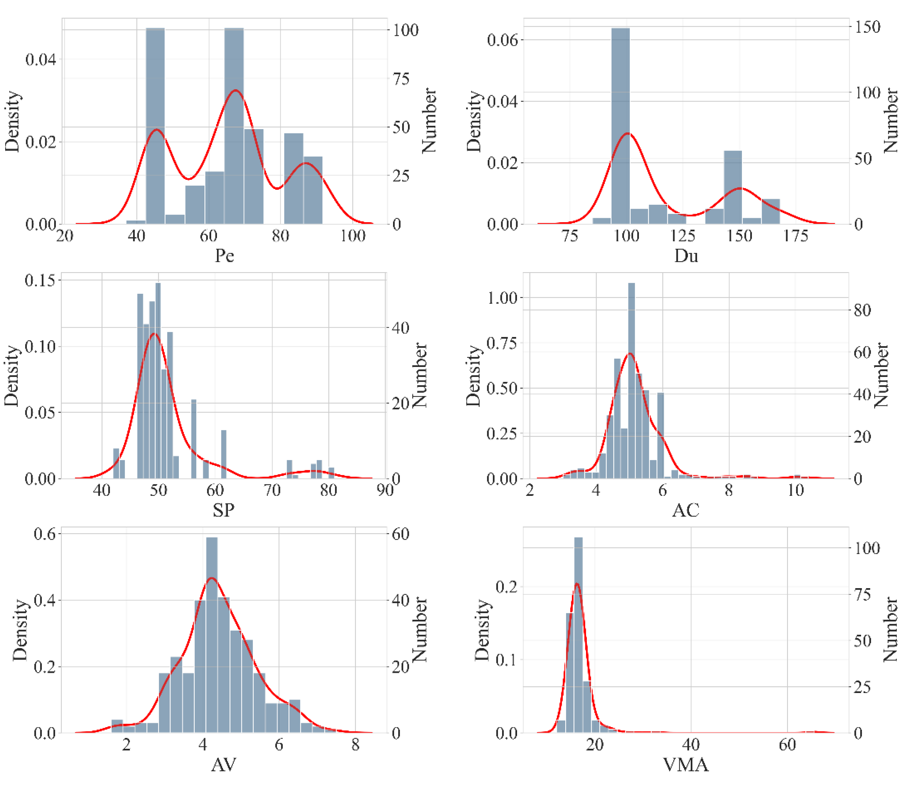
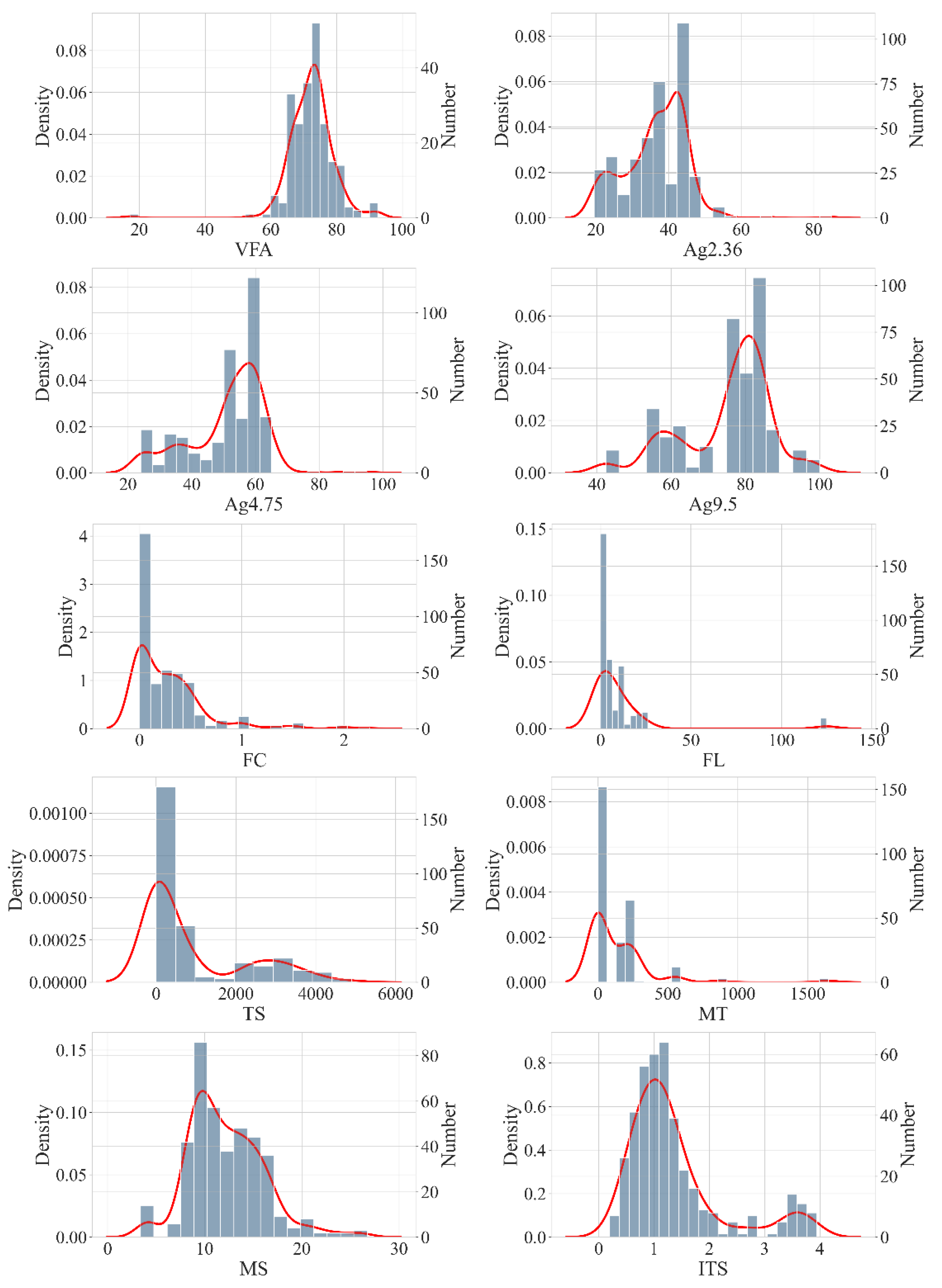
Table A2.
Summary of out-of-sample predictive accuracy across 20 Monte Carlo splits.
| Model | Metrics | ||||
| RMSE | MAE | MAPE | MAD | R2 | |
| TabPFN | 0.94 ± 0.12 | 0.61 ± 0.06 | 9.98 ± 1.30 | 0.41 ± 0.06 | 0.87 ± 0.04 |
| TabICLv2 | 0.94 ± 0.15 | 0.61 ± 0.07 | 10.24 ± 1.64 | 0.40 ± 0.05 | 0.87 ± 0.04 |
| RF | 1.00 ± 0.14 | 0.67 ± 0.08 | 13.50 ± 2.49 | 0.44 ± 0.06 | 0.85 ± 0.04 |
| XGBoost | 1.01 ± 0.12 | 0.68 ± 0.07 | 12.88 ± 2.38 | 0.45 ± 0.06 | 0.84 ± 0.04 |
Table A3.
Transposed full feature information of the observed-data Pareto solutions.
| Feature | E134 | E275 | E277 | E124 | E041 | E251 | E278 | E279 | E081 | E138 |
| Rank | 1 | 2 | 3 | 4 | 5 | 5 | 7 | 8 | 9 | 10 |
| FT | Mineral fiber | Carbon fiber | Carbon fiber | Mineral fiber | Plastic fiber | Plastic fiber | Carbon fiber | Carbon fiber | No fiber | Plastic fiber |
| Pe | 91.6 | 60 | 60 | 91.8 | 85.9 | 85.9 | 60 | 60 | 47 | 57 |
| Du | 150.00 | 100.00 | 100.00 | 150.00 | 100.00 | 100.00 | 100.00 | 100.00 | 100.00 | NA |
| SP | 46.90 | 42.00 | 42.00 | 49.60 | 46.50 | 46.50 | 42.00 | 42.00 | 61.00 | 51.60 |
| AC | 5.27 | 6.20 | 6.50 | 5.80 | 3.80 | 4.00 | 5.90 | 6.70 | 4.30 | 4.65 |
| AV | 3.10 | 4.89 | 5.29 | 3.36 | 3.81 | 3.81 | 7.01 | 6.08 | 3.90 | 4.41 |
| VMA | 14.20 | 14.84 | 15.19 | 16.75 | NA | NA | 17.69 | 15.90 | 12.10 | NA |
| VFA | 78.60 | 67.03 | 65.20 | 79.94 | NA | NA | 60.35 | 61.78 | 67.77 | NA |
| Ag2.36 | 33.9 | 37.7 | 37.7 | 37 | 23 | 23 | 37.7 | 37.7 | 26.6 | 39.06 |
| Ag4.75 | 54.8 | 54 | 54 | 53 | 33.5 | 33.5 | 54 | 54 | 37.9 | 48.63 |
| Ag9.5 | 80.9 | 79.1 | 79.1 | 76.5 | 55.5 | 55.5 | 79.1 | 79.1 | 58.3 | 76.27 |
| FC | 0.2 | 0.4 | 0.6 | 0.3 | 0.23 | 0.23 | 0.8 | 0.8 | 0 | 0.075 |
| FL | 6 | 6 | 6 | 6 | 6 | 0.02 | 6 | 6 | 0 | 4 |
| TS | 2320 | 3500 | 3500 | 2320 | 591 | 591 | 3500 | 3500 | 0 | 780 |
| MT | NA | NA | NA | NA | 259 | 259 | NA | NA | 0 | NA |
| MS | 15.23 | 26.72 | 24.95 | 13.06 | 10.78 | 10.78 | 20.55 | 19.22 | 15.26 | 15.56 |
| ITS | 3.9 | 1.66 | 1.76 | 3.91 | 3.94 | 3.94 | 1.9 | 2.06 | 2.71 | 2.34 |
| TOPSIS score | 0.55 | 0.54 | 0.52 | 0.50 | 0.46 | 0.46 | 0.42 | 0.39 | 0.36 | 0.30 |
References
- Wang, F.; Hoff, I.; Yang, F.; Wu, S.; Xie, J.; Li, N.; Zhang, L. Comparative assessments for environmental impacts from three advanced asphalt pavement construction cases. J. Clean. Prod. 2021, 297, 126659. [Google Scholar] [CrossRef]
- AlKheder, S.; AlKandari, D.; AlYatama, S. Sustainable assessment criteria for airport runway material selection: A fuzzy analytical hierarchy approach. Eng. Constr. Archit. Manag. 2022, 29, 3091–3113. [Google Scholar] [CrossRef]
- James, W.; Thompson, M.K. Contaminants from four new pervious and impervious pavements in a parking-lot. In Advances in Modeling the Management of Stormwater Impacts; CRC Press, 2021; pp. 207–222. [Google Scholar] [CrossRef]
- Ning, Z.; Sun, Z.; Liu, Y.; Dong, J.; Meng, X.; Wang, Q.; Wei, Y. Evaluating the impervious performance of hydraulic asphalt concrete in embankment dams: A study of crack evolution at different temperatures. Constr. Build. Mater. 2024, 440, 137247. [Google Scholar] [CrossRef]
- Bieliatynskyi, A.; Yang, S.; Pershakov, V.; Shao, M.; Ta, M. Features of the hot recycling method used to repair asphalt concrete pavements. Mater. Sci.-Pol. 2022, 40, 181–195. [Google Scholar] [CrossRef]
- Yao, H.; Wang, Y.; Ma, P.; Li, X.; You, Z. A literature review: Asphalt pavement repair technologies and materials. Proc. Inst. Civ. Eng. Eng. Sustain. 2023, 177, 259–273. [Google Scholar] [CrossRef]
- Rivera-Perez, J.; Talebpour, A.; Al-Qadi, I.L. Prediction of asphalt concrete flexibility index and rut depth utilising deep learning and Monte Carlo Dropout simulation. Int. J. Pavement Eng. 2023, 24, 2253964. [Google Scholar] [CrossRef]
- Ma, R.; Li, Y.; Cheng, P.; Chen, X.; Cheng, A. Low-temperature cracking and improvement methods for asphalt pavement in cold regions: A review. Buildings 2024, 14, 3802. [Google Scholar] [CrossRef]
- Al-Atroush, M.E. Structural behavior of the geothermo-electrical asphalt pavement: A critical review concerning climate change. Heliyon 2022, 8, e12107. [Google Scholar] [CrossRef] [PubMed]
- Arabzadeh, A.; Ceylan, H.; Kim, S.; Gopalakrishnan, K.; Sassani, A. Superhydrophobic coatings on asphalt concrete surfaces: Toward smart solutions for winter pavement maintenance. Transp. Res. Rec. 2016, 2551, 10–17. [Google Scholar] [CrossRef]
- American Society for Testing and Materials. ASTM D6927-15; Standard Test Method for Marshall Stability and Flow of Asphalt Mixtures. ASTM International: West Conshohocken, PA, USA, 2015. [CrossRef]
- ASTM International. ASTM D6931-17; Standard Test Method for Indirect Tensile (IDT) Strength of Asphalt Mixtures. ASTM International: West Conshohocken, PA, USA, 2017. [CrossRef]
- Dias, J.F.; Picado-Santos, L.G.; Capitao, S.D. Mechanical performance of dry process fine crumb rubber asphalt mixtures placed on the Portuguese road network. Constr. Build. Mater. 2014, 73, 247–254. [Google Scholar] [CrossRef]
- Zaumanis, M.; Mallick, R.B.; Frank, R. 100% hot mix asphalt recycling: Challenges and benefits. Transp. Res. Procedia 2016, 14, 3493–3502. [Google Scholar] [CrossRef]
- Liu, Q.T.; Wu, S.P. Effects of steel wool distribution on properties of porous asphalt concrete. Key Eng. Mater. 2014, 599, 150–154. [Google Scholar] [CrossRef]
- Garcia, A.; Norambuena-Contreras, J.; Bueno, M.; Partl, M.N. Influence of steel wool fibers on the mechanical, termal, and healing properties of dense asphalt concrete. J. Test. Eval. 2014, 42, 1107–1118. [Google Scholar] [CrossRef]
- Pasandin, A.R.; Perez, I. Overview of bituminous mixtures made with recycled concrete aggregates. Constr. Build. Mater. 2015, 74, 151–161. [Google Scholar] [CrossRef]
- Wang, L.; Zhang, J.; Song, M.; Tian, B.; Li, K.; Liang, Y.; Han, J.; Wu, Z. A shell-crosslinked polymeric micelle system for pH/redox dual stimuli-triggered DOX on-demand release and enhanced antitumor activity. Colloids Surf. B Biointerfaces 2017, 152, 1–11. [Google Scholar] [CrossRef] [PubMed]
- Awan, H.H.; Hussain, A.; Javed, M.F.; Qiu, Y.; Alrowais, R.; Mohamed, A.M.; Fathi, D.; Alzahrani, A.M. Predicting Marshall flow and Marshall stability of asphalt pavements using multi expression programming. Buildings 2022, 12, 314. [Google Scholar] [CrossRef]
- Rahman, S.; Bhasin, A.; Smit, A. Exploring the use of machine learning to predict metrics related to asphalt mixture performance. Constr. Build. Mater. 2021, 295, 123585. [Google Scholar] [CrossRef]
- Liu, J.; Liu, F.; Wang, L. Acceleration of superpave mix design: Solving multi-objective optimization problems using machine learning and the non-dominated sorting genetic Algorithm-II. Transp. Res. Rec. 2024, 2678, 1863–1886. [Google Scholar] [CrossRef]
- Zhang, J.; Huang, Y.; Wang, Y.; Ma, G. Multi-objective optimization of concrete mixture proportions using machine learning and metaheuristic algorithms. Constr. Build. Mater. 2020, 253, 119208. [Google Scholar] [CrossRef]
- Guo, P.; Meng, W.; Xu, M.; Li, V.C.; Bao, Y. Predicting mechanical properties of high-performance fiber-reinforced cementitious composites by integrating micromechanics and machine learning. Materials 2021, 14, 3143. [Google Scholar] [CrossRef] [PubMed]
- Guo, P.; Meng, W.; Bao, Y. Knowledge-guided data-driven design of ultra-high-performance geopolymer (UHPG). Cem. Concr. Compos. 2024, 153, 105723. [Google Scholar] [CrossRef]
- Tan, X.; Xing, J.; Wang, Y.; Qiu, H.; Mahjoubi, S.; Guo, P. Explainable machine learning for predicting compressive strength of rubberized concrete: SHAP interpretation, lifecycle assessment, and design recommendations. J. Clean. Prod. 2026, 538, 147338. [Google Scholar] [CrossRef]
- Tan, X.; Xing, J.; Mahjoubi, S.; Guo, P.; Wei, Z.; Wang, Y.; Ren, J.; Ai, L.; Meng, W.; Bao, Y. Explainable machine learning and life cycle assessment for sustainable design of fiber-reinforced asphalt concrete. J. Clean. Prod. 2026, 547, 147759. [Google Scholar] [CrossRef]
- Xing, J.; Tan, X.; Li, Y.; Jin, D.; Guo, P.; Wang, Y.; Niu, H. Interpretable machine learning for predicting splitting strength of asphalt concrete: Insights from SHAP analysis. Materials 2026, 19, 1636. [Google Scholar] [CrossRef] [PubMed]
- Probst, P.; Boulesteix, A.L.; Bischl, B. Tunability: Importance of hyperparameters of machine learning algorithms. J. Mach. Learn. Res. 2019, 20, 1–32. [Google Scholar]
- Zahoor, M.F.; Hussain, A.; Khattak, A. Machine learning-based prediction performance comparison of Marshall Stability and flow in asphalt mixtures. Infrastructures 2025, 10, 142. [Google Scholar] [CrossRef]
- Hollmann, N.; Muller, S.; Purucker, L.; Krishnakumar, A.; Korfer, M.; Hoo, S.B.; Schirrmeister, R.T.; Hutter, F. Accurate predictions on small data with a tabular foundation model. Nature 2025, 637, 319–326. [Google Scholar] [CrossRef] [PubMed]
- Qu, J.; Holzmuller, D.; Varoquaux, G.; Morvan, M.L. TabICLv2: A better, faster, scalable, and open tabular foundation model. arXiv 2026, arXiv:2602.11139. [Google Scholar] [CrossRef]
- Abd, N.I.; Latief, R.H. The effects of fibers on the properties of local hot asphalt mixtures. Tikrit J. Eng. Sci. 2024, 31, 146–157. [Google Scholar] [CrossRef]
- Aboutalebi Esfahani, M.; Namavar Jahromi, M. Optimum parafibre length according to mechanical properties in hot mix asphalt. Road. Mater. Pavement Des. 2020, 21, 683–700. [Google Scholar] [CrossRef]
- Ai, C. Characteristics and Design Methods of Asphalt Pavement in Plateau-Cold Region . Ph.D. Thesis, Southwest Jiaotong University, Chengdu, China, 2008. Available online: https://cdmd.cnki.com.cn/Article/CDMD-10613-2008177745.htm.
- Al-Ridha, A.S.; Alkaissi, Z.A.; Kareem, S.M. Evaluating the influence of adding steel fibers on the moisture damage and aging resistance of hot asphalt mixtures. Mater. Today Proc. 2021, 47, 2520–2528. [Google Scholar] [CrossRef]
- Al-Ridha, A.S.; Ibrahim, S.K.; Dheyab, E.L.S. Steel fiber effect on the behavior of hot mixture asphalt with variable asphalt content. Int. J. Adv. Technol. Eng. Sci. 2016, 4, 204–213. Available online: https://www.researchgate.net/publication/329586636.
- Al-Saadi, A.A.; Ismael, M.Q. Improvement of moisture susceptibility for asphalt mixture with ceramic fiber. J. Eng. 2023, 29, 78–91. [Google Scholar] [CrossRef]
- Ali, S.; Siddiqui, M.O.R.; Ahmed, A.; Iqbal, K.; Noorani, M.U.; Sun, D.; Iqbal, W. Performance evaluation of hot mix asphalt using textile waste. Ind. Text. 2022, 73, 225–232. [Google Scholar] [CrossRef]
- Aljubory, A.; Teama, Z.T.; Salman, H.T.; Abd Alkareem, H.M. Effects of cellulose fibers on the properties of asphalt mixtures. Mater. Today Proc. 2021, 42, 2941–2947. [Google Scholar] [CrossRef]
- Burak, S.; Ali, T. Use of asphalt roofing shingle waste in HMA. Constr. Build. Mater. 2005, 19, 337–346. [Google Scholar] [CrossRef]
- Chen, F.; Xue, J.; Yang, Z.; Gao, K.; Huo, Z. Influence of wood fiber on the laboratory road performance of recycled asphalt pavement (RAP) asphalt mixture. IOP Conf. Ser. Mater. Sci. Eng. 2020, 772, 012025. [Google Scholar] [CrossRef]
- Chen, Z.; Chen, Z.; Yi, J.; Feng, D. Preparation method of corn stalk fiber material and its performance investigation in asphalt concrete. Sustainability 2019, 11, 4050. [Google Scholar] [CrossRef]
- Chen, M. Research on Snow Melting and Solar Energy Collection for Thermal Conductive Asphalt Pavement . Ph.D. Thesis, Wuhan University of Technology, Wuhan, China, 2012. Available online: https://cdmd.cnki.com.cn/Article/CDMD-10497-1012442416.htm.
- Cheng, Y.; Li, L.; Zhou, P.; Zhang, Y.; Liu, H. Multi-objective optimization design and test of compound diatomite and basalt fiber asphalt mixture. Materials 2019, 12, 1461. [Google Scholar] [CrossRef] [PubMed]
- Dalhat, M.A.; Osman, S.A.; Alhuraish, A.A.A.; Almarshad, F.K.; Qarwan, S.A.; Adesina, A.Y. Chicken feather fiber modified hot mix asphalt concrete: Rutting performance, durability, mechanical and volumetric properties. Constr. Build. Mater. 2020, 239, 117849. [Google Scholar] [CrossRef]
- Esfandiarpour, S. Hybrid Reinforcement of Asphalt-Concrete Mixtures Using Glass and Polypropylene Fibers . Doctoral Dissertation, Eastern Mediterranean University, Famagusta, Cyprus, 2010. Available online: http://hdl.handle.net/11129/149.
- Fan, T.; Si, C.; Zhang, Y.; Zhu, Y.; Li, S. Optimization design of asphalt mixture composite reinforced with calcium sulfate anhydrous whisker and polyester fiber based on response surface methodology. Materials 2023, 16, 594. [Google Scholar] [CrossRef] [PubMed]
- Fan, T. Study on Performance of Calcium Sulfate Whisker-Polyester Fiber Compound Modified Asphalt and Asphalt Mixture . Ph.D. Thesis, Changan University, Xi'an, China, 2020. [Google Scholar] [CrossRef]
- Gui-juan, Z. Test on evaluation index of deformation performance for polyester fiber reinforced asphalt concrete. Proceedings of the 2010 International Conference on Intelligent System Design and Engineering Application 2010, Volume 2, 561–564. [Google Scholar] [CrossRef]
- He, Y.; Zhang, J.; Zhao, X.; Wang, M.; Xiong, K.; Hu, Q. Study on design optimization, road performance verification and preparation process selection of hybrid fiber reinforced asphalt mixture composite. Constr. Build. Mater. 2024, 448, 138245. [Google Scholar] [CrossRef]
- Hidayat, N.; Pratama, G.N.I.P.; Pramita, I.D. The effect of PET plastic addition (polyethylene terephthalate) and carbide waste filler for asphalt concrete-binder course (AC-BC) on Marshall characteristics. IOP Conf. Ser. Earth Environ. Sci. 2019, 366, 012024. [Google Scholar] [CrossRef]
- Hussein, F.K.; Ismael, M.Q.; Huseien, G.F. Rock wool fiber-reinforced and recycled concrete aggregate-imbued hot asphalt mixtures: Design and moisture susceptibility evaluation. J. Compos. Sci. 2023, 7, 428. [Google Scholar] [CrossRef]
- Kim, M.J.; Kim, S.; Yoo, D.Y.; Shin, H.O. Enhancing mechanical properties of asphalt concrete using synthetic fibers. Constr. Build. Mater. 2018, 178, 233–243. [Google Scholar] [CrossRef]
- Kumar, P.; Mehndiratta, H.C.; Immadi, S. Investigation of fiber-modified bituminous mixes. Transp. Res. Rec. 2009, 2126, 91–99. [Google Scholar] [CrossRef]
- Li, C. Study on the Self-Healing Performance and Mechanism of Asphalt Concrete Under Microwave Radiation . Ph.D. Thesis, Wuhan University of Technology, Wuhan, China, 2020. [Google Scholar] [CrossRef]
- Li, H.; Liang, D.; Xiao, Z.; Chen, M.; Zhao, W. Performance characterization of steel slag powder and its effect on the water stability of asphalt concrete. J. Wuhan Univ. Technol. Transp. Sci. Eng. 2020, 44, 536–540. [Google Scholar]
- Liu, F.; Dong, A.; Liu, C.; Wu, W. Mix design of asphalt mixture used for the waterproof and anti-cracking layer in the rainy area of South China. J. Appl. Biomater. Funct. Mater. 2018, 16, 112–118. [Google Scholar] [CrossRef] [PubMed]
- Liu, X.; Yu, X.M.; Xu, C.; Chu, J.W. The research of durability of asphalt concrete bridge deck with little polyester fiber content in cold regions. Key Eng. Mater. 2020, 852, 41–48. [Google Scholar] [CrossRef]
- Ma, Z. Design and Application Research of Electrically Heated Ice and Snow Melting Paving Structure Based on Conductive Rubber Composite Material . Ph.D. Thesis, Jilin University, Changchun, China, 2024. [Google Scholar] [CrossRef]
- Mawat, H.Q.; Ismael, M.Q. Assessment of moisture susceptibility for asphalt mixtures modified by carbon fibers. Civ. Eng. J. 2020, 6, 304–317. [Google Scholar] [CrossRef]
- Miera-Dominguez, H.; Lastra-Gonzalez, P.; Indacoechea-Vega, I.; Castro-Fresno, D. Evaluation of the mechanical performance of AC mixtures with recycled fibres. Dev. Built Environ. 2024, 18, 100435. [Google Scholar] [CrossRef]
- Moussa, G.K.; Gomaa, K. Effect of addition of short fibers of poly-acrylic and polyamide to asphalt mixtures. Alex. Eng. J. 2003, 42, 329–336. [Google Scholar]
- Pratul, R.; Satish, K.; Kumar, S.A. Experimental study on fiber reinforced bituminous concrete. Mater. Today Proc. 2021, 46, 11077–11083. [Google Scholar] [CrossRef]
- Qin, L. Study on the effects of aging on the volume and water stability properties of steel slag and its asphalt concrete. J. China Foreign Highw. 2019, 39, 264–270. [Google Scholar] [CrossRef]
- Shanbara, H.K. Effect of carbon fiber on the performance of reinforced asphalt concrete mixture. Muthanna J. Eng. Technol. 2011, 1, 39–51. [Google Scholar] [CrossRef]
- Shu, J.; Xv, K.; Liu, S.; Wan, P.; Liu, Q.; Wu, S. Effects of calcium alginate/Fe3O4 composite self-healing capsules on road performance of asphalt concrete. J. Wuhan Univ. Technol. Transp. Sci. Eng. 2025, 1–17. Available online: https://link.cnki.net/urlid/42.1824.U.20250325.1426.00.
- Singh, S.; Khairandish, M.I.; Razahi, M.M.; Kumar, R.; Chohan, J.S.; Tiwary, A.; Sharma, S.; Li, C.; Ilyas, R.A.; Asyraf, M.R.M.; Zakaria, S.Z.S. Preference index of sustainable natural fibers in stone matrix asphalt mixture using waste marble. Materials 2022, 15, 2729. [Google Scholar] [CrossRef] [PubMed]
- Slebi-Acevedo, C.J.; Lastra-Gonzalez, P.; Castro-Fresno, D.; Vega-Zamanillo, A. Experimental evaluation and recyclability potential of asphalt concrete mixtures with polyacrylonitrile fibers. Constr. Build. Mater. 2022, 317, 125829. [Google Scholar] [CrossRef]
- Tu, Y.; Chen, G.; Cheng, Z.; Cheng, S. Effect of nano-SiO2 on properties of recycled aggregate asphalt mixture. Mater. Rep. 2022, 36, 220–224. [Google Scholar]
- Wang, X.; Zhou, H.; Hu, X.; Shen, S.; Dong, B. Investigation of the performance of ceramic fiber modified asphalt mixture. Adv. Civ. Eng. 2021, 2021, 8833468. [Google Scholar] [CrossRef]
- Wu, C.; Li, L.; Cheng, Y.; Gu, Z.; Lv, Z.; Wang, R.; Guan, B. Effect of diatomite and basalt fibers on pavement performance and vibration attenuation of waste tires rubber-modified asphalt mixtures. Math. Probl. Eng. 2020, 2020, 8853428. [Google Scholar] [CrossRef]
- Yin, J.; Wu, W. Utilization of waste nylon wire in stone matrix asphalt mixtures. Waste Manag. 2018, 78, 948–954. [Google Scholar] [CrossRef] [PubMed]
- Zhao, S.Q. Study on short carbon fiber asphalt concrete Marshall. Adv. Mater. Res. 2012, 529, 446–449. [Google Scholar] [CrossRef]
- Paraskevas, K.; Christos, T. Data preprocessing and feature engineering for data mining: Techniques, tools, and best practices. AI 2025, 6, 257. [Google Scholar] [CrossRef]
- Breiman, L. Random forests. Mach. Learn. 2001, 45, 5–32. [Google Scholar] [CrossRef]
- Chen, T.; Guestrin, C. XGBoost: A scalable tree boosting system. In Proceedings of the 22nd ACM SIGKDD International Conference on Knowledge Discovery and Data Mining, San Francisco, CA, USA, 13-17 August 2016; Association for Computing Machinery: New York, NY, USA, 2016; pp. 785–794. [Google Scholar] [CrossRef]
- Akiba, T.; Sano, S.; Yanase, T.; Ohta, T.; Koyama, M. Optuna: A next-generation hyperparameter optimization framework. In Proceedings of the 25th ACM SIGKDD International Conference on Knowledge Discovery and Data Mining, Anchorage, AK, USA, 4-8 August 2019; pp. 2623–2631. [Google Scholar] [CrossRef]
- Deb, K.; Pratap, A.; Agarwal, S.; Meyarivan, T. A fast and elitist multiobjective genetic algorithm: NSGA-II. IEEE Trans. Evol. Comput. 2002, 6, 182–197. [Google Scholar] [CrossRef]
- Hwang, C.-L.; Yoon, K. Multiple Attribute Decision Making: Methods and Applications: A State-of-the-Art Survey; Springer: Berlin/Heidelberg, Germany, 1981. [Google Scholar] [CrossRef]
- Behzadian, M.; Otaghsara, S.K.; Yazdani, M.; Ignatius, J. A state-of-the-art survey of TOPSIS applications. Expert Syst. Appl. 2012, 39, 13051–13069. [Google Scholar] [CrossRef]
- Lundberg, S.M.; Lee, S.I. A unified approach to interpreting model predictions. Adv. Neural Inf. Process. Syst. 2017, 30. [Google Scholar] [CrossRef]
Figure 1.
General research framework.
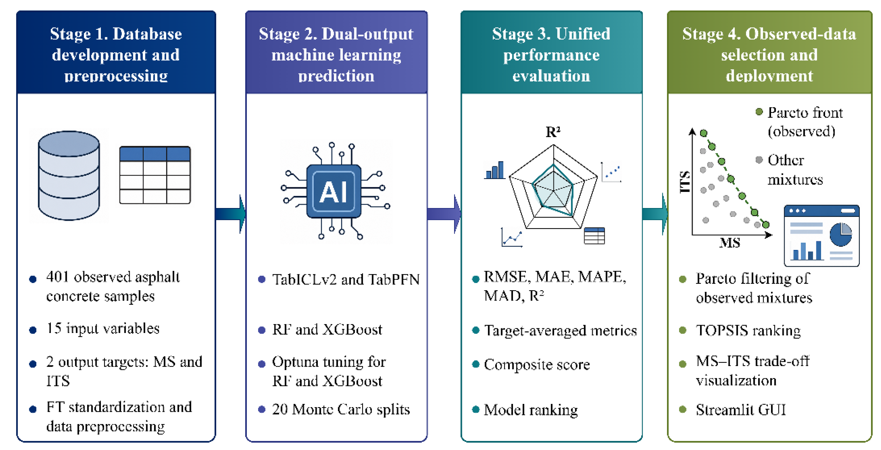
Figure 2.
Correlation analysis of input and output variables.
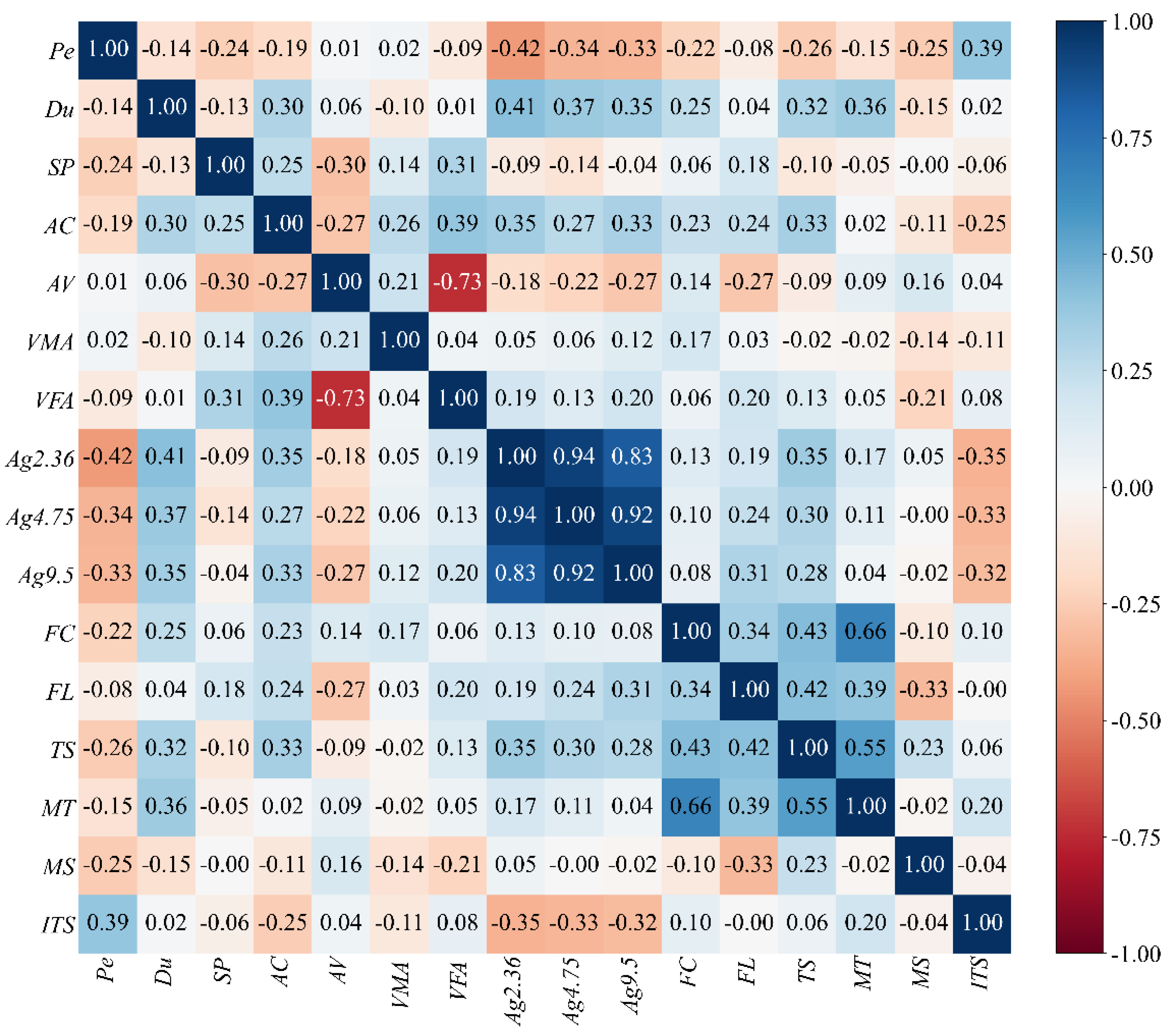
Figure 3.
Comparison of traditional machine learning and tabular foundation models.
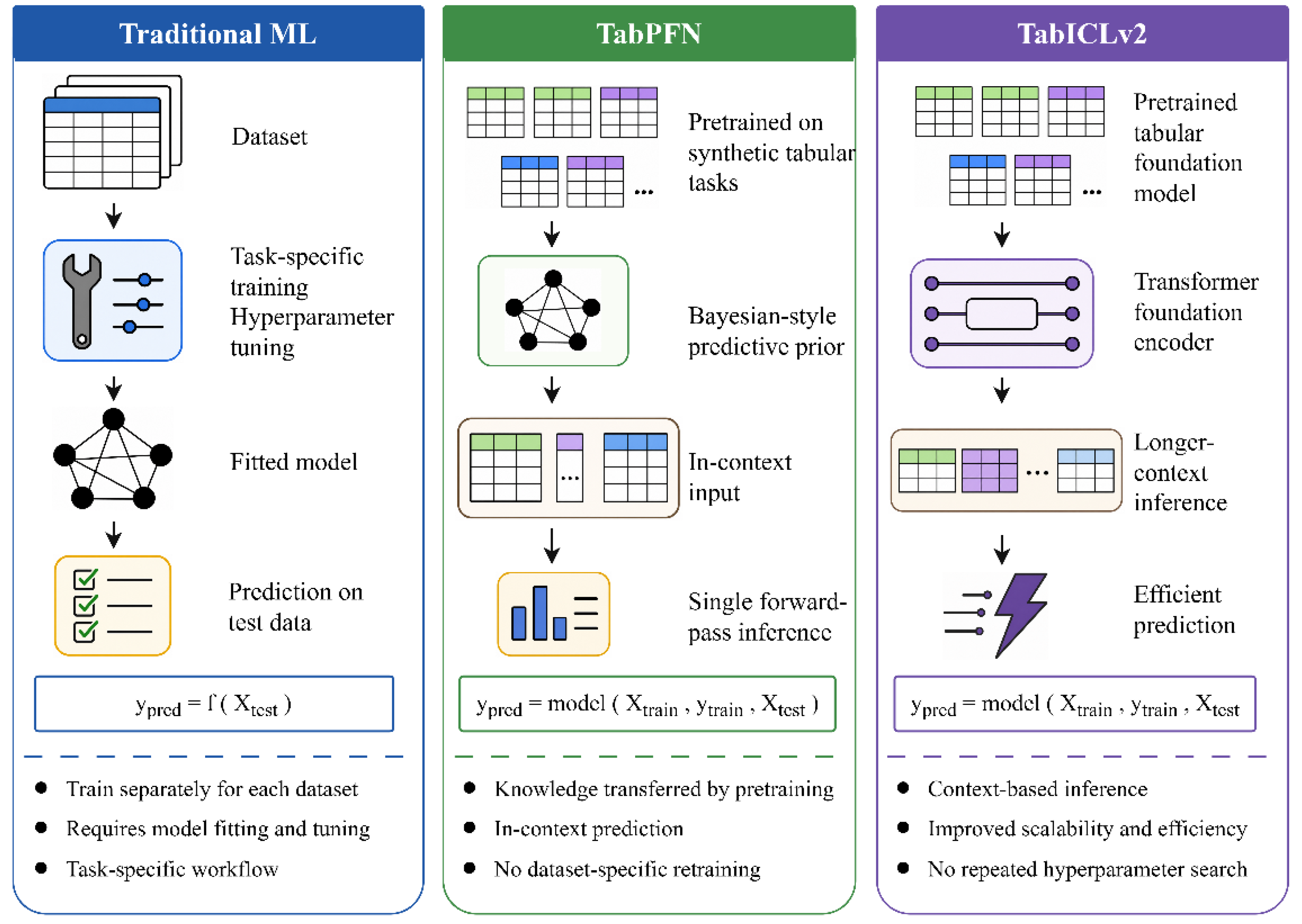
Figure 4.
Workflow of Optuna-based hyperparameter tuning for tree-based models.
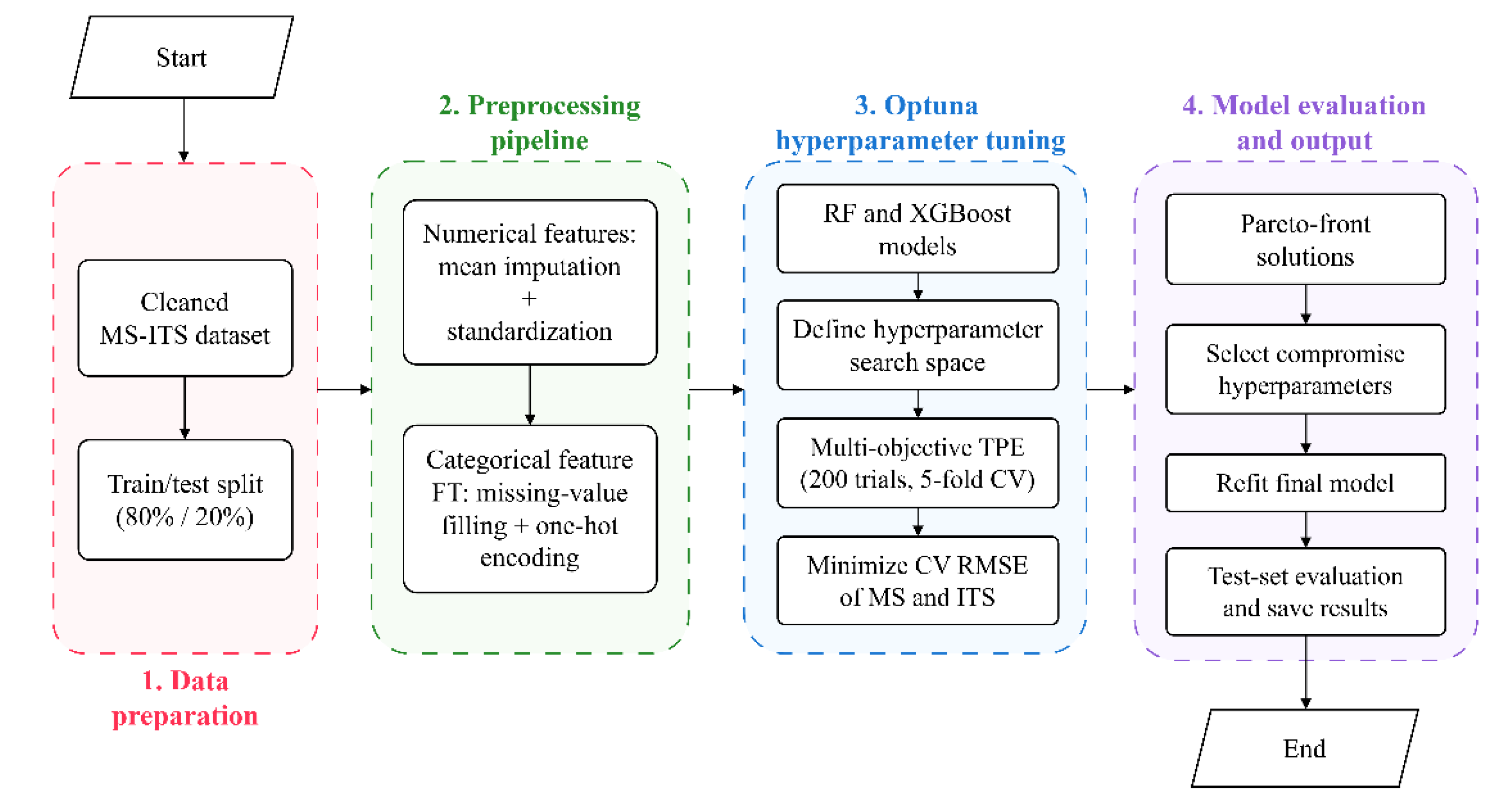
Figure 5.
Workflow of observed-data Pareto filtering and TOPSIS-based mixture selection.
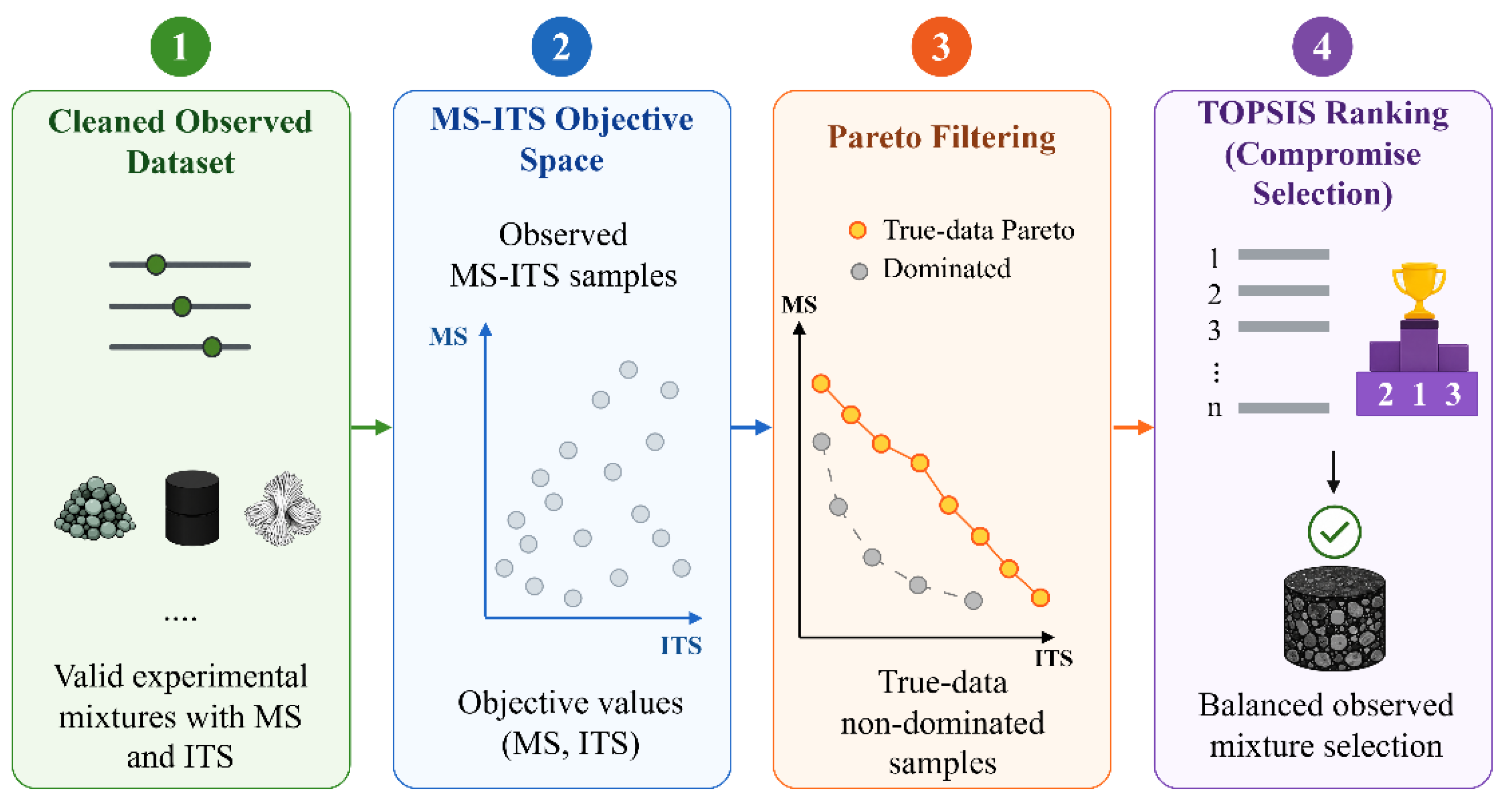
Figure 6.
Optimization histories of RF and XGBoost during Optuna tuning.
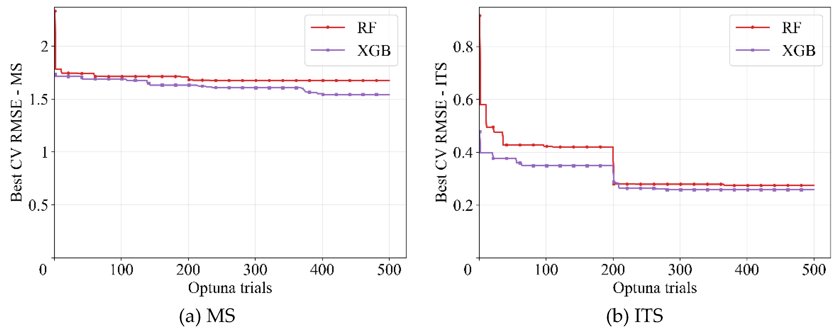
Figure 7.
Measured and predicted values of MS and ITS for different models.
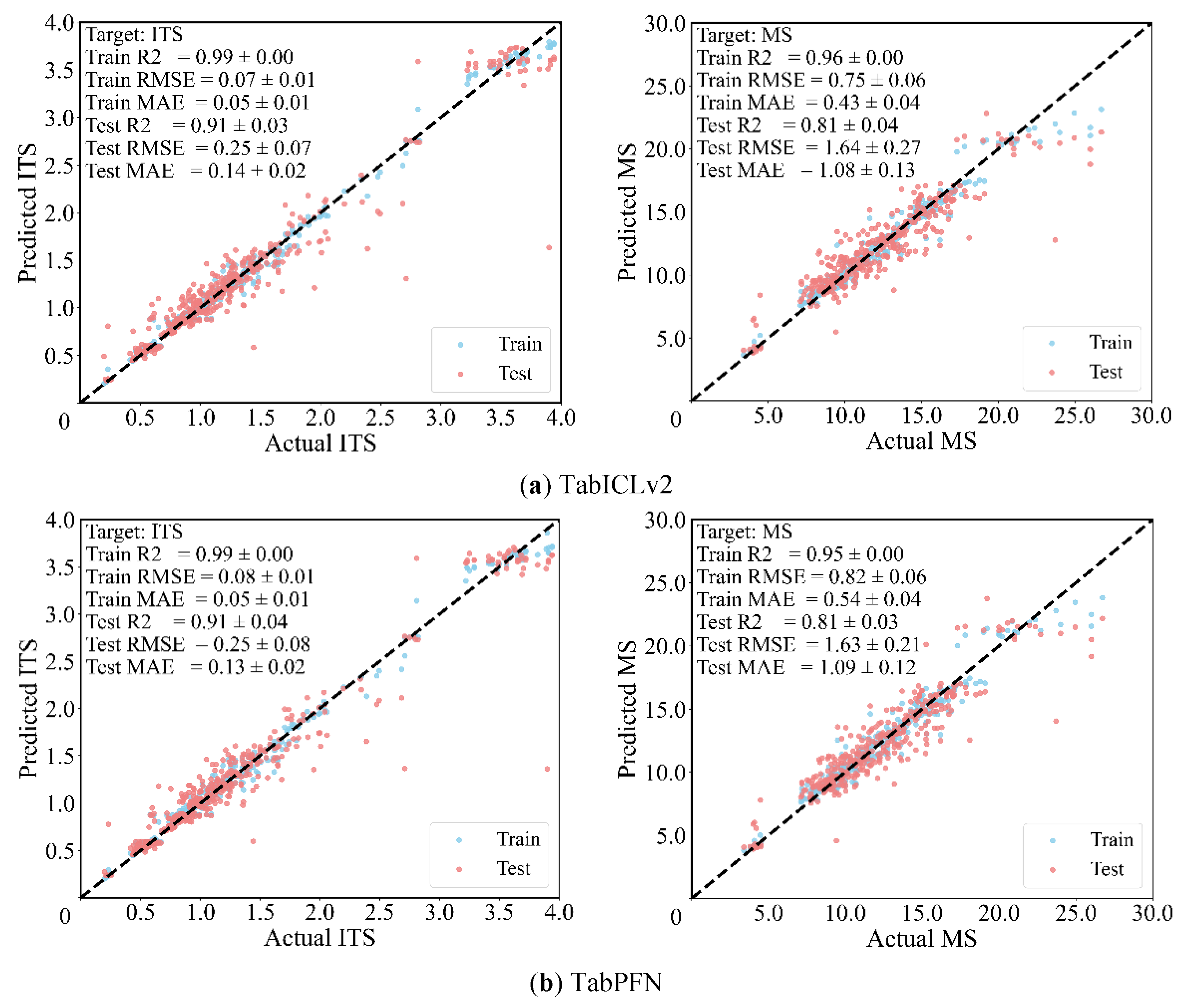
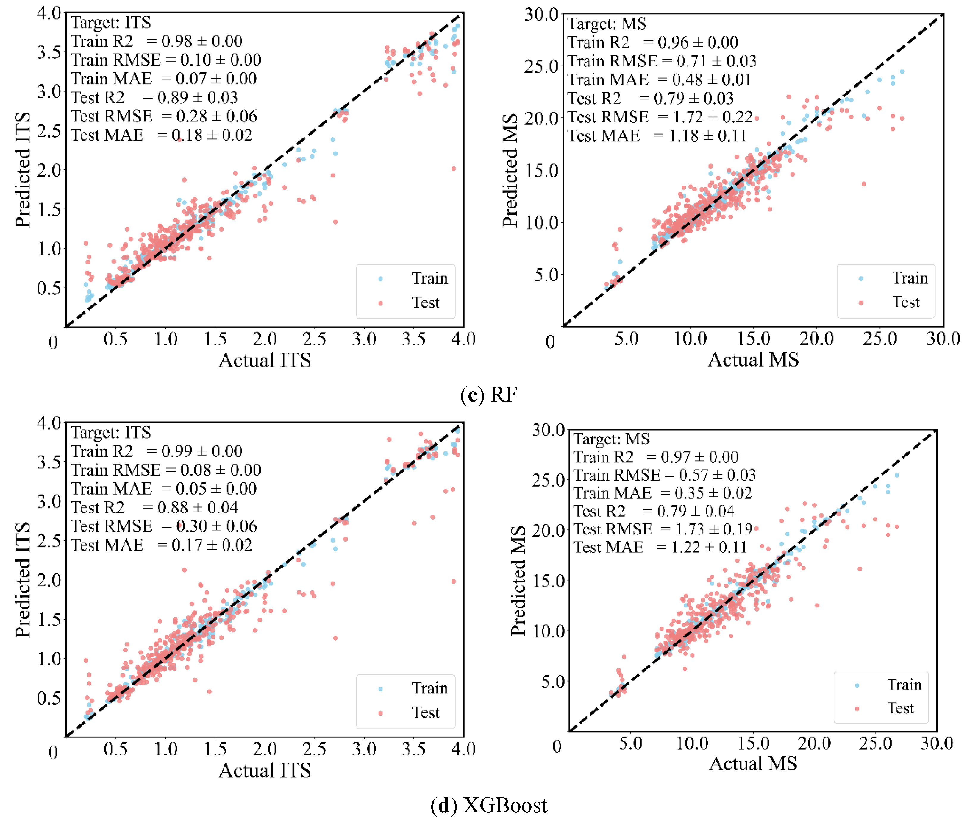
Figure 8.
Comprehensive comparison of model performance based on multiple metrics.
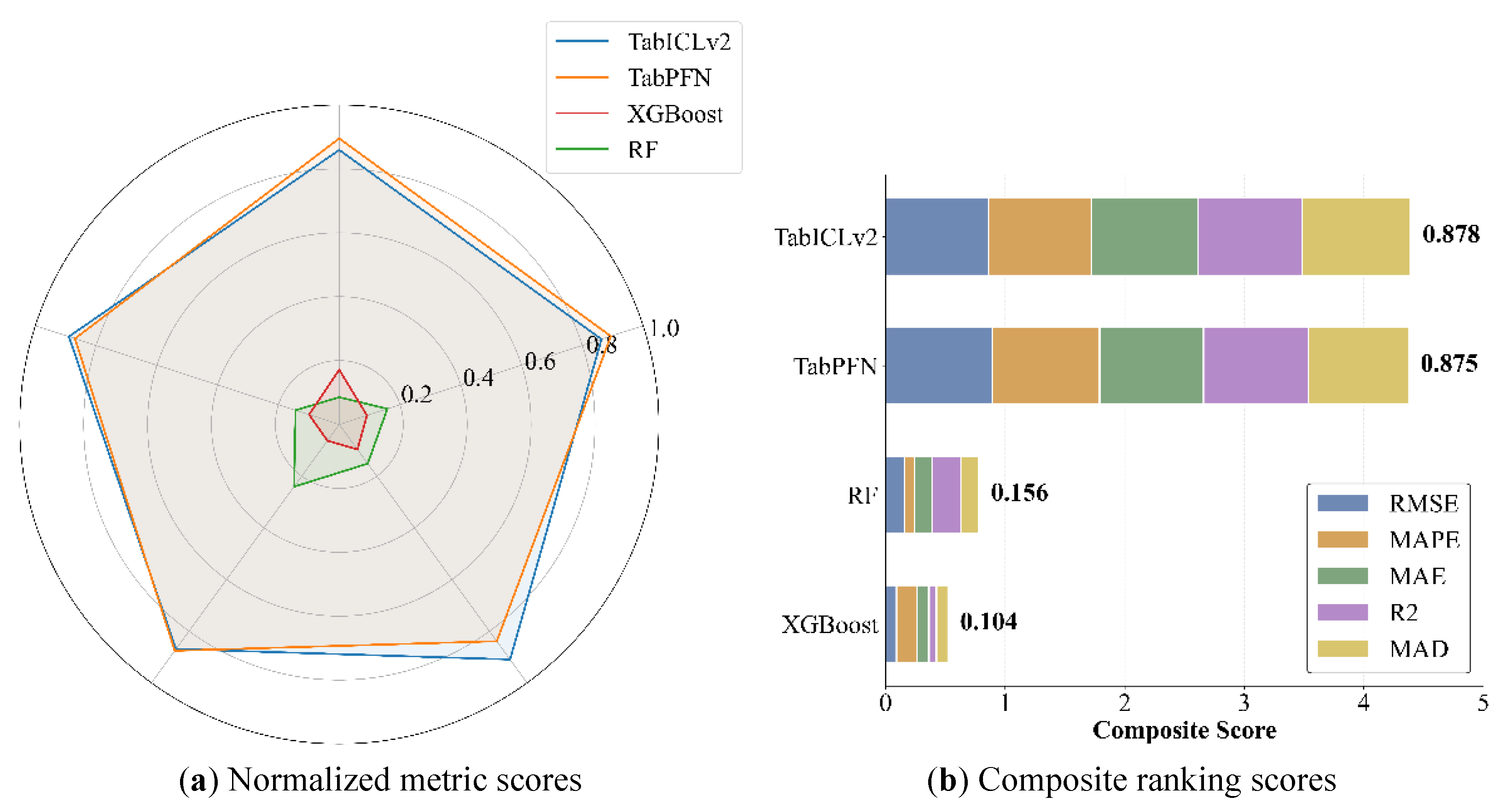
Figure 9.
Pareto front and TOPSIS selection for observed MS-ITS data.
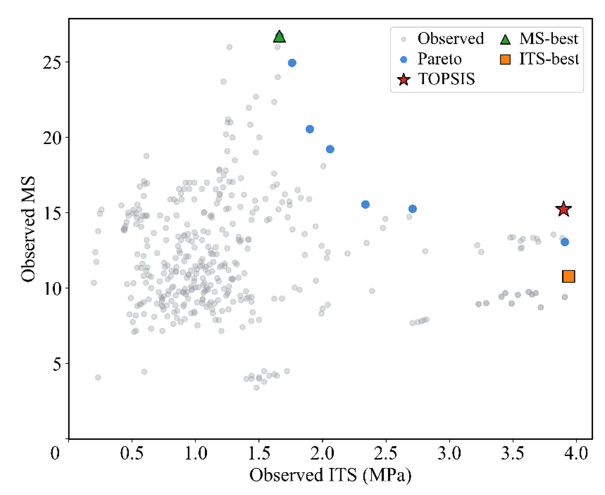
Figure 10.
Streamlit-based GUI for MS and ITS prediction and interpretation.
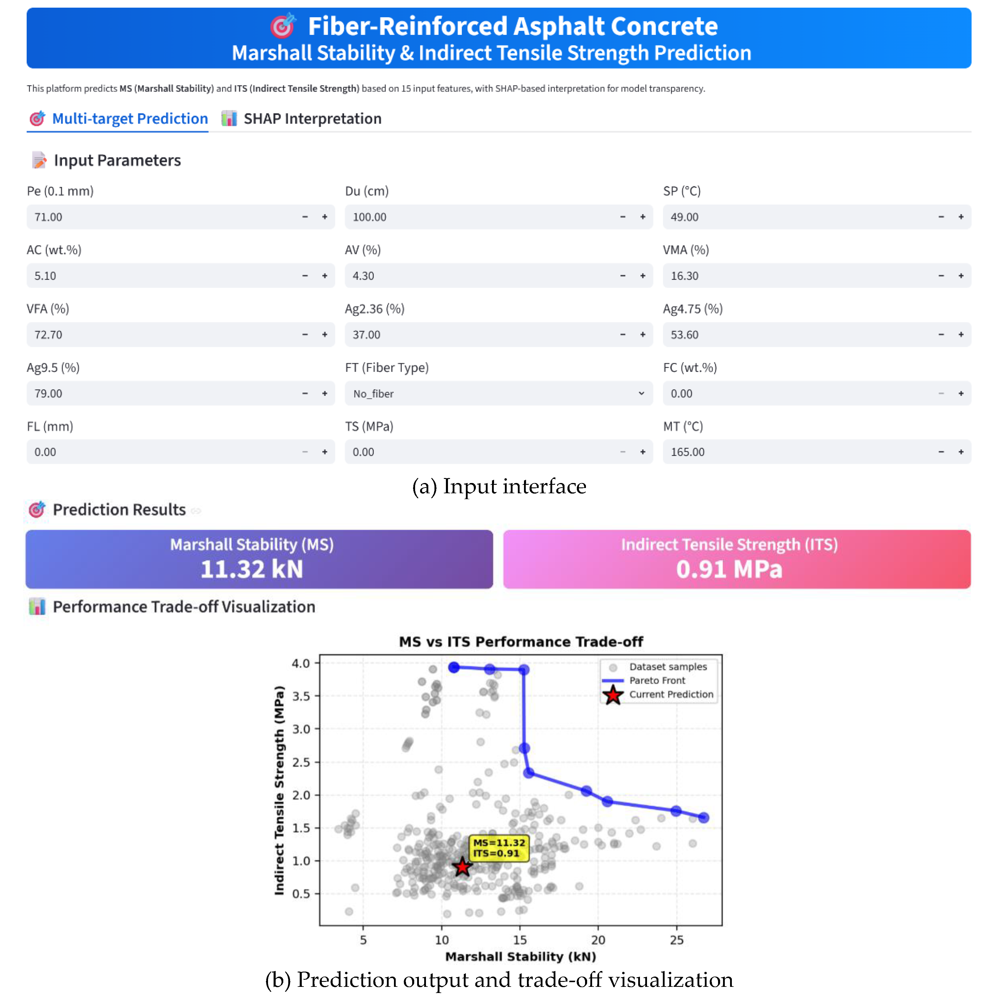
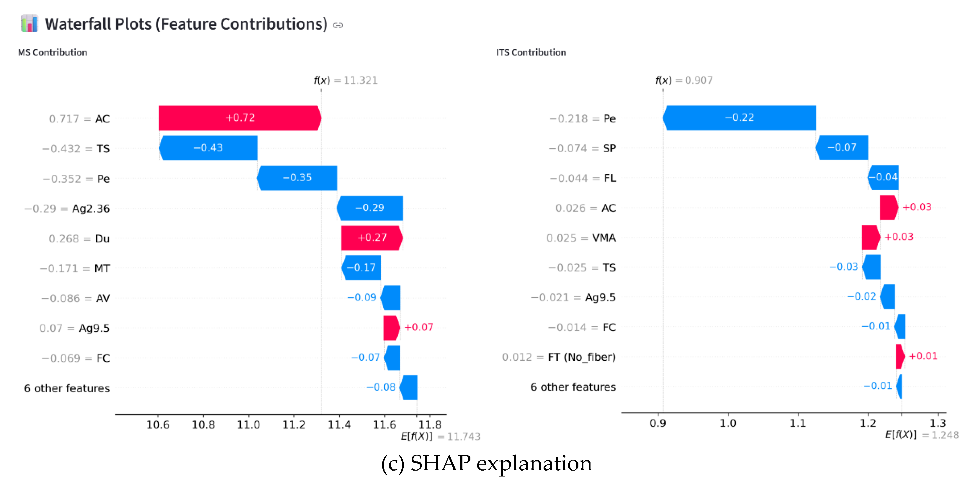
Table 1.
Overview of fiber categories and their amounts.
| Fiber categories | Sample size |
| Plastic fiber | 122 |
| Mineral fiber | 41 |
| Bio-fiber | 36 |
| Carbon fiber | 19 |
| Glass fiber | 16 |
| Steel fiber | 15 |
| No fiber | 152 |
Table 2.
Descriptive statistics of input and output variables.
| Variable | Unit | Min | Q1 | Q2 | Q3 | Max | Mean | STD |
| Pe | 0.1 mm | 37 | 47 | 65.12 | 71.6 | 91.8 | 64.92 | 15.06 |
| Du | cm | 85 | 100 | 100 | 150 | 168 | 118.36 | 24.7 |
| SP | °C | 42 | 48 | 49.6 | 51.6 | 81 | 51.56 | 7.03 |
| AC | wt.% | 3 | 4.7 | 5 | 5.5 | 10.39 | 5.16 | 0.85 |
| AV | % | 1.6 | 3.9 | 4.31 | 5 | 7.5 | 4.42 | 0.98 |
| VMA | % | 12.1 | 15.5 | 16.34 | 17.27 | 65.6 | 16.83 | 3.92 |
| VFA | % | 17.11 | 68.19 | 72.67 | 75.17 | 92.5 | 72.32 | 6.93 |
| Ag2.36 | % | 19.45 | 30.39 | 37 | 42.84 | 85 | 36.42 | 8.55 |
| Ag4.75 | % | 24 | 45.54 | 53.65 | 59.18 | 95 | 51.1 | 11.74 |
| Ag9.5 | % | 42.5 | 69 | 79 | 82.92 | 100 | 75.26 | 11.94 |
| FT | / | / | / | / | / | / | / | / |
| FC | wt.% | 0 | 0 | 0.2 | 0.4 | 2.25 | 0.27 | 0.35 |
| FL | mm | 0 | 0 | 4 | 12 | 125 | 9.19 | 20.5 |
| TS | MPa | 0 | 0 | 33 | 1700 | 4900 | 906.59 | 1306 |
| MT | °C | 0 | 0 | 0 | 220 | 1650 | 131.91 | 230.95 |
| MS | kN | 3.4 | 9.43 | 11.52 | 14.7 | 26.72 | 12.18 | 3.85 |
| ITS | MPa | 0.2 | 0.83 | 1.12 | 1.5 | 3.94 | 1.36 | 0.87 |
Table 3.
Overview of machine learning models.
| No. | Model | Category | Notes |
| 1 | TabICLv2 | Foundation model | Pretrained transformer for tabular prediction |
| 2 | TabPFN | Foundation model | In-context learning for tabular regression |
| 3 | RF | Ensemble—Bagging | Bagging of decision trees |
| 4 | XGBoost | Ensemble—Boosting | Boosting model with regularization |
Table 4.
Model configurations and optimized hyperparameter settings.
| Models | Hyperparameters |
| TabICLv2 | default hyperparameters; device = cuda if available, otherwise cpu |
| TabPFN | default hyperparameters; device = cuda if available, otherwise cpu |
| RF | n_estimators = 194; max_depth = 28; min_samples_split = 2; min_samples_leaf = 1; max_features = 1.0; bootstrap = True; random_state = 42; n_jobs = -1 |
| XGBoost | n_estimators = 447; max_depth = 4; learning_rate = 0.09; reg_alpha = 0.00; reg_lambda = 3.89; min_child_weight = 3.31; objective = reg:squarederror; tree_method = hist; random_state = 42; n_jobs = -1; verbosity = 0 |
Table 5.
Design-oriented summary of observed-data Pareto solutions.
| Design pathway | Representative Pareto solutions | Fiber system | FC (%) | FL (mm) | AC (%) | MS (kN) | ITS (MPa) | Design implication |
| Balanced MS-ITS | E134, E124 | Mineral fiber / basalt | 0.20-0.30 | 6.00 | 5.27-5.80 | 13.06-15.23 | 3.90-3.91 | Candidate window for balanced mechanical performance |
| MS-dominant | E275, E277, E278, E279 | Carbon fiber / carbon | 0.40-0.80 | 6.00 | 5.90-6.70 | 19.22-26.72 | 1.66-2.06 | High MS, but lower ITS should be expected |
| ITS-dominant | E041, E251 | Plastic fiber / polyester | 0.23 | 0.02 or 6.00 | 3.80-4.00 | 10.78 | 3.94 | High ITS, but MS compensation may be required |
| No-fiber reference | E081 | No fiber | 0.00 | 0.00 | 4.30 | 15.26 | 2.71 | Non-fiber Pareto baseline |
| Plastic-fiber reference | E138 | Plastic fiber / polyacrylonitrile | 0.075 | 4.00 | 4.65 | 15.56 | 2.34 | Additional lower-ranked Pareto option |
| Note: The ranges in Table 5 were derived from the observed-data Pareto solutions grouped by design role. | ||||||||
Disclaimer/Publisher’s Note: The statements, opinions and data contained in all publications are solely those of the individual author(s) and contributor(s) and not of MDPI and/or the editor(s). MDPI and/or the editor(s) disclaim responsibility for any injury to people or property resulting from any ideas, methods, instructions or products referred to in the content. |
© 2026 by the authors. Licensee MDPI, Basel, Switzerland. This article is an open access article distributed under the terms and conditions of the Creative Commons Attribution (CC BY) license.
Copyright: This open access article is published under a Creative Commons CC BY 4.0 license, which permit the free download, distribution, and reuse, provided that the author and preprint are cited in any reuse.


