Preprint
Article

This version is not peer-reviewed.

Seawater Acidification and Bubble Plume Dispersion from Accidental Subsea CO₂ Pipeline Rupture: A Multiphase CFD Study

Submitted:

01 July 2026

Posted:

01 July 2026

You are already at the latest version

Abstract

The ecology and maritime traffic safety would be at risk if a CO₂ reservoir or transmission pipeline were to leak. To address this need, multiphase Computational Fluid Dynamics (CFD) models were developed using ANSYS Fluent to predict these coupled processes. The 3D Eulerian-Eulerian CFD model has been developed for validation and the 2D model for predicting the 50m case. The physical and chemical processes involved, such as buoyancy, turbulence, and gas dissolution kinetics, are all considered. The mass transfer coefficient is estimated using the Hughmark correlation. Seawater temperature and salinity are used for estimating dissociation and Henry’s Law constant. The 3D model is validated with the QICS and Hauser Tank Experiments. Hypothetical CO2 release from High Island 10L was simulated and compared to prior work. Findings indicate that the water column can fully mitigate a CO2 release of 35 kg/s in 50 m of water due to CO2 absorption in seawater during ascent. The CFD simulations offer understanding of environmental impact including bubble plume behavior, dissolution into the water column, and consequent changes in seawater pH and pCO₂ and a framework for evaluating CO2 leak impacts on marine environments in the Gulf of Mexico.
Keywords: 
;  ;  ;  ;  ;  

1. Introduction

Marchetti (1977) proposed a CO2 management system involving collection, transport, and long-term storage in deep rock layers beneath the ocean. This leads to the modern concept of Carbon Capture and Storage (CCS) that sequestrates carbon dioxide produced by various industrial sources, such as electric power generation and natural gas processing, to prevent its release into the atmosphere [1]. The CO2 transportation from the sources to the final destinations and CO2 storage may involve pipelines, barges, trucks, etc. Each step of the handling process including transport, injection, storage and utilization carries a risk of leakage. Pipeline failures are a critical threat to energy networks, causing severe environmental contamination, supply chain disruptions, and risks to public safety. The leakage of submarine CO2 creates serious hazards such as dangerous gas plumes and pollution of ocean waters [2]. Subsea CO2 pipeline ruptures or leakages pose a potential hazard for the safety of ships, offshore infrastructure and for the marine ecosystems. If CO2 leaks from subsea pipelines or storage reservoirs, it can lead to asphyxiating or poisonous atmospheric conditions,., alternation of the dissolved inorganic carbon (DIC), partial pressure of CO2 (pCO2), and decrease in pH which threaten marine ecosystems [3,4].
Subsea leaks can be classified into three types based on their leakage rates: severe leaks (exceeding 10 kg/s), moderate leaks (1 to 10 kg/s), and small leaks (0.1 to 1 kg/s). Minor leaks frequently remain hidden for a long time [2]. Due to recent occurrences and events, law and corporate regulations require formal risk evaluations of underwater gas leaks. A subsea gas release brought on by a breach puts at risk the integrity of the safety assets and the operational safety of an offshore third party. We need a better understanding of how underwater gas escapes and disperses to address such accidents. In this work, the risk and impact of potential CO2 leakages from pipelines connected to storage reservoirs into the water column were investigated.
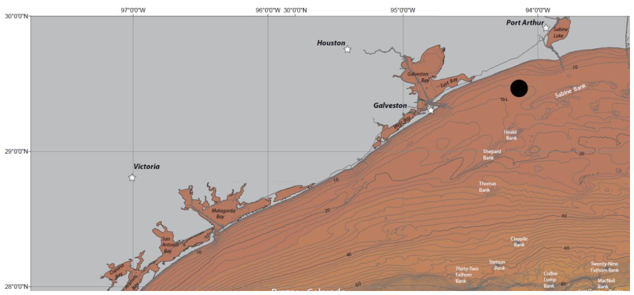
The Miocene formations in the offshore Texas Gulf of Mexico offer excellent reservoir quality, effective sealing layers, and appropriate subsurface conditions for underground CO2 storage (Ramirez, 2019). The High Island 10-L field, a depleted oil and gas reservoir in Texas State Waters, has been identified as a potential site for CCS of industrial CO₂ emissions, including those from Beaumont-Port Arthur Refineries, about 25 miles away. The lower Miocene sands of the Fleming Group exhibit porosities of 29–33 % and permeabilities of 465–790 mD, while the overlying Amphistegina B shale and multiple intra-formational mud layers act as regional and secondary seals, respectively. The reservoir depth of approximately 1.2–2.6 km ensures CO₂ would be in a supercritical phase, enhancing storage efficiency. High Island 10-L also contributes to assessing the broader Texas–Louisiana Gulf of Mexico Miocene strata, which contain more than two-thirds of the estimated U.S. CO₂ storage resources. Modeling estimates the P₅₀ CO₂ storage capacity of the field at 37.56–40.39 Mt, confirming its potential for large scale geological storage.
Figure 1. Bathymetric of the northwestern Gulf of Mexico, High Island 10L Location. [5].
Preprints 221053 g001
Oldenburg [4] reported that the water column at a depth of 50 meters could entirely absorb CO2​ from a major blowout, though the resulting pH changes were not investigated. Researchers at the University of Tokyo (UOT) adapted an existing Eulerian-Lagrangian (E-L) model, originally designed for CO2​ droplets in the deep ocean, by modifying its drag and mass transfer coefficients to simulate the behavior and termination of CO2​ bubbles in shallow water [6,7]. The Eulerian–Lagrangian (E–L) model tracks individual CO₂ bubbles and droplets, solving their motion and mass conservation equations. Bubble size evolution due to dissolution is explicitly calculated, with drag and mass transfer coefficients updated dynamically based on instantaneous volume and shape. The model does not employ a population balance equation, and interactions such as coalescence or breakup are not considered. Dewar et al. employed all-scale Eulerian-Eulerian (E-E) model developed at Heriot-Watt University to simulate the plume behavior and dissolution of CO2​ bubbles rising from sediments into the shallow waters of the North Sea. The model did not consider bubble breakup and coalescence [8,9].
This research aims to address that knowledge gap with a strong emphasis on CO2 mass transfer, chemisorption, and model validation. In other words, this study looks into the changes in pH and the partial pressure of CO2​ (pCO2​) that would result from a hypothetical leak at the High Island 10L Well. Our CFD model has been validated with two experimental data sets: (1) the Quantifying and Monitoring Potential Ecosystem Impacts of Geological Carbon Storage (QICS) research initiative on monitoring ecosystem responses to subsurface carbon storage [10,11,12] and (2) the Huser Tank experiment (Huser, 2016). These experiments furnish essential insights in the intricate dynamics of CO2 transport during leakage incidents. Afterwards, the validated model was used to compare with Oldenburg's work [4] and then predicts other scenarios on the High Island 10L case.

2. Mathematical Modeling

2.1. Eulerian Model

The Eulerian multiphase model in ANSYS Fluent (2023) enables the simulation of systems involving multiple interacting phases, such as gas–liquid (CO2–seawater) flows. This model is based on the Eulerian–Eulerian (E–E) approach, in which both the continuous and dispersed phases are treated as interpenetrating continua rather than discrete elements. Within this framework, phasic volume fractions are introduced to represent the spatial occupancy of each phase, and conservation equations (including continuity and momentum) are solved for every phase [11]. In this study, multiphase flow is simulated numerically using Ansys Fluent. The detailed model equations are presented in the Supplementary.
The continuity equation is expressed as follows:
t α q ρ q + α q ρ q v q = p = 1 n m ˙ p q m ˙ q p + S q
In Eq. (1), v q is the velocity of phase q, m ˙ p q and m ˙ q p represent the mass transfer rate from the pth to the qth phase and vice versa respectively , S q is the source term (default value of zero), and α q is volumetric fraction of phase q.
The momentum equation is expressed as follows:
t α q ρ q v q + α q ρ q v q v q = α q p + τ q + α q ρ q g + F q + F l i f t , q + F v m , q p = 1 n R p q + m ˙ p q v p q m ˙ q p v q p
In Eq. (2), F q , F l i f t , q , F v m , q , R p q is external body force, lift force, virtual mass, interaction force respectively, τ q is stress-strain tensor, μ q and λ q is shear and bulk viscosity respectively, p is the pressure shared by all phases, v q p is the interphase velocity. Further details are provided in Supplementary Section S1.

2.2. Drag and Lift Force

Pham et al. [13] relied solely on the Tomiyama model for its established capability to address bubble shape effects on both drag and lift coefficients, as the complexity observed in the QICS experiment, where CO2​ bubbles exhibited a range of shapes (sphere, cap, and ellipse), necessitates a specialized approach [14]. In the present work, the Grace et al. model, that models drag across varying bubble shapes and flow regimes by leveraging the Reynolds and Eötvös numbers, was implemented for the drag force calculation. Then the Tomiyama et al. model was utilized for the lift force, capitalizing on its unique strength in predicting the lift coefficient (CL​) and the critical cross-over point caused by particle distortion. This dual-model approach allows us to combine the most robust and accurate correlations for drag and lift forces, providing a more reliable and physically consistent simulation of the CO2​ dispersion dynamics. Additional definitions are given in Supplementary Section S2.

2.3. Turbulence Model

Both interfacial force and turbulence models were employed to represent multiphase flow behavior in this study. The interfacial force formulations (drag force and lift force) are strongly influenced by turbulence characteristics; therefore, accurate turbulence modeling is essential. The standard k–ε model, while widely used, tends to overpredict gas holdup near walls because of its isotropic eddy viscosity assumption. This limitation can be addressed by employing the realizable k–ε model [12]. In this study, the Shear Stress Transport (SST) k–ω model is adopted, blending the k–ω formulation near the wall for improved boundary-layer resolution with the k–ε formulation in the bulk flow for stable far-field predictions. This hybrid approach enhances the prediction of gas volume fraction and interfacial momentum exchange, leading to better agreement with experimental data, such as the Hauser Tank validation and the 50 m case [15,16]. The equations are given below:
t ρ k + x i ρ k u i = x j Γ k k x j + G k Y k + S k + G b
t ρ ω + x j ρ ω u j = x j Γ ω ω x j + G ω Y ω + D ω + S ω + G ω b
Where Gk is the generation of turbulence kinetic energy due to the mean velocity gradients, Gω is the generation of ω, Γk is effective diffusivity of k. Γω is the effective diffusivity of ω, Yk is the dissipation of k, Yω is the dissipation of ω, Dω is cross-diffusion, and Sk and Sω are user-defined source terms.
The transport equations for the standard k-e model are based on the turbulence kinetic energy (k) and its dissipation rate (e). Eq. (5) and (6) describe the transport equations used in the turbulent model standard k- e [16,17].
( ρ k ) t + x i ρ k u i = x j ( μ t σ k + μ ) k x j + G k + G b ρ ε Y M + S k
( ρ ε ) t + x i ρ ε u i = x j ( μ t σ ε + μ ) ε x j + C 1 ε ε k G k + C 3 ε G b C 2 ε ρ ε 2 k + S ε
Where Gk represents the generation of turbulence kinetic energy resulting from mean velocity gradients, Gb ​accounts for the influence of buoyancy on turbulence production. The dilatation term YM captures the effects of compressibility on the dissipation rate. Model constants C, C and C ​ define the empirical relationships in the dissipation equation, and the turbulent Prandtl numbers σk and σε ​ correspond to the transport of k and ε, respectively. Additional user-defined source terms, Sk and Sε​, can be incorporated to represent specific physical phenomena or boundary effects [17,18].
Table 1. Default values of model constant C, C, Cμ, σk and σε.
Model Constants C C Cμ σk σε
Default Value 1.44 1.92 0.09 1.0 1.3

2.4. Mass Transfer Model

Accurate simulation of gas–liquid mass transfer requires careful selection of the mass transfer coefficient, which reflects the combined effects of diffusion, convection, bubble size, flow conditions, and surface characteristics [19]. Because interphase transfer can be complex, multi-component species transfer cannot be represented accurately using a single overall coefficient. Whitman’s two-resistance (or Two-Film) model addresses this by considering the separate contributions of the gas and liquid phases to the overall resistance [17]. The following equation can describe mass transfer:
m ˙ q = K L A C q , s C q
where m ˙ q denotes the mass transfer rate (kg/s), KL is the overall mass transfer coefficient (m/s), A represents the interfacial area (m²), Cq,s ​ is the concentration of the species at the interface, and Cq ​ is its concentration in the seawater phase (kg/m3). The overall mass transfer coefficient KL ​ is given by:
1 K L = 1 k L + 1 k G H c
where kG is the mass transfer coefficient of the gas phase (m/s) and Hc denotes Henry’s law constant.
In many practical cases, such as the transfer of sparingly soluble gases like CO₂ in water, the gas-phase resistance is negligible, and the liquid boundary layer governs the transfer through Fickian diffusion, driving species down the concentration gradient [17].
The overall mass transfer can be expressed as:
1 K L = 1 k L
The bubble radius is an important factor in determining mass transfer from a CO₂ bubble to seawater. The Sherwood number characterizes the combined effects of convection and diffusion at the interface; the boundary layer thickness is set by the local convective conditions and relative transport rates in the two phases. In this study, the Hughmark correlation is used to estimate the mass transfer coefficient and is expressed as:
S h = 2 + 0.95 Re 1 2 S c 1 3 D d b
where Sh is the Sherwood number, Sc is the Schmidt number, Re is the Reynolds number, db is the bubble diameter and D is diffusivity. The definitions of the terms are given in Supplementary Section S3.

2.5. Chemical Reaction Model

Dissolved CO2 gas reacts with seawater, generating H+ that decreases seawater pH [20]. Three distinct inorganic forms of carbon dioxide may be found in the ocean: aqueous carbon dioxide, bicarbonate ion, and carbonate ion. Carbonic acid is a fourth form; however, its concentration (0.3%) is substantially lower than that of aqueous carbon dioxide.
The mechanisms responsible for the dissolution of gaseous CO2 into seawater and the subsequent hydration and dehydration reactions of dissolved CO₂ are outlined below. The CO₂ gas first dissolves physically into seawater:
CO2(g) ⇌ CO2(aq) (R1)
Dissolved CO₂ then undergoes hydration and stepwise dissociation:
CO2(aq) + H2O ⇌ H2CO3 ⇌ H+ + HCO3- ⇌ 2 H+ + CO32- (R2)
A key step in the alkaline mechanism involves dissolved CO2 reacting with OH- to produce HCO3- [20].
CO2 + OH- ⇌ HCO3- (R3)
Bicarbonate may further react with hydroxide to yield carbonate and water:
HCO3- + OH- ⇌ CO32- + H2O (R4)
Consequently, the carbonate system in seawater comprises five primary components: CO2(aq), HCO3-, CO32-, H+ and OH- in this investigation. The initial concentrations of these species are calculated from the measured total alkalinity (TA) and pH, with temperature (T) and salinity (S) used to determine the relevant stoichiometric dissociation constants and equilibrium constants. In the simulation, these calculated concentrations are then assigned as the initial mass fractions.
The species concentrations are determined as follows:
H + = 10 p H s w
H C O 3 = T A H + + H + 2 K W S w H + + 2 K 2 S W
C O 3 2 = K 2 S W H C O 3 H +
C O 2 ( a q ) = H C O 3 H + K 1 S W
O H = K w s w H +
See Supplementary section S4 for the chemical definition of TA and equilibrium constants.
Once the aqueous carbonate system is defined, the solubility of CO₂ in water must be determined to relate these concentrations to the gas phase. Henry’s law coefficient provides this link. Eq. (16) is used to calculate Henry’s law constant of CO2 in pure water ( H C O 2 , W ). This value then serves as the basis for estimating the coefficient in seawater ( H C O 2 , S W ) by incorporating the effects of salinity. The foundational equation for CO2​ solubility in pure water is given below [21]:
log H C O 2 , W = 108.3865 + 0.01985076 T 6919.53 T 40.45154 l o g T + 669365 T 2
H C O 2 , W is calculated in   m o l   k g . a t m , and T (temperature) is a range which is valid up to 607.15 K. This step is essential as it establishes solubility dependence on temperature.
Due to the presence of dissolved salts, which reduce gas solubility in water, a phenomenon known as salting out, the Henry’s law coefficient in saline solutions, such as seawater ( H G , S W ) , can be obtained by adjusting the value for pure water ( H G , W ) at the same temperature using the Sechenov relation , as expressed by Danckwerts [22].
log H G , S W H G , W = I h
where I is the ionic strength of the solution and h is defined as:
h = h + + h + h G
Using Eq. (17), H C O 2 , S W can be calculated. Once H C O 2 , S W   is known, the partial pressure of CO₂ in equilibrium with seawater is given in Eq. (19):
p C O 2 = C C O 2 H C O 2 . S W

2.6. Population Balance Model

The Population Balance Equation (PBE) provides a comprehensive mathematical framework for modeling dispersed phase with a particular focus on gas bubbles of different sizes. The key element of this model is the number density function, which describes how many CO2 bubbles exist at a given size or condition, and how these numbers change over time. This change is quantified through birth and death functions, which account for discrete changes in particle numbers caused by phenomena such as aggregation and breakage. Additionally, the model considers how variations in bubble size distribution influence the properties of the surrounding fluid and gas phases.
This change is quantified through two primary mechanisms: growth, which represents for continuous changes in particle properties over time, and birth-and-death, which represents discrete changes in particle numbers due to phenomena such as aggregation (coalescence) and breakage (splitting). These mechanisms together capture the evolution of the particle size distribution in the system. Additionally, the model considers how variations in bubble size distribution influence the properties of the surrounding fluid and gas phases [11].
The general form of the Population Balance Equation can be written as:
t [ n ( V , t ) ] + [ u n ( V , t ) ] + v G v n ( V , t ) { G r o w t h t e r m } =
1 2 0 V a V V ' , V ' n V V ' , t n V ' , t d V ' { B i r t h d u e t o A g g r e g a t i o n } 0 a V , V ' n ( V , t ) n V ' , t d V ' { D e a t h d u e t o A g g r e g a t i o n }
+ Ω v p g V ' β V V ' n V ' , t d V ' { B i r t h d u e t o B r e a k a g e } g V n V , t D e a t h d u e t o B r e a k a g e
The initial and boundary conditions are specified as follows:
n V , t = 0 = n v
n ( V = 0 , t ) G v = n ˙ 0
Here, n ˙ 0 is the nucleation rate (particles/m3s)

2.6.1. Particle Growth

The particle volume-based growth rate, G v (m³/s), and the particle diameter-based growth rate are, respectively, expressed as:
G v = V t
G = L t
The volume of a single particle V is expressed as K v L 3 , where L   is the characteristic particle length (or diameter). Therefore, the relationship between G v and G is:
G v = 3 K v L 2 G

2.6.2. Particle Birth and Death

In this work, the breakage model proposed by Ramakrishna [23] and the aggregation kernel by Luo [24] are used.
The breakage rate is given by:
B b i = i N n i , k g v k N k
Where
n i , k = v i v i + 1 v i + 1 v v i + 1 v i β v k , v d v + v i 1 v i v v i 1 v i v i 1 β v k , v d v
The Luo model’s general aggregation kernel is defined as the rate at which particle volume is generated due to binary collisions between particles of volumes Vi and Vj:
Ω a g V i , V j = ω a g V i , V j P a g V i , V j [ m 3 s ]
Here, ω a g V i , V j represents the collision frequency and P a g V i , V j   denotes the likelihood of coalescence after a collision. Additional technical specifications are provided in Supplementary section S5.

3. Results

This section presents the results of the CFD simulations and their validation against experimental datasets, offering a detailed understanding of subsea gas release phenomena and demonstrating the reliability of the simulation methodology. The study focuses on simulating subsea CO₂ discharge in the Gulf of Mexico using CFD. To ensure the accuracy of the results, the model was validated against two well-known experimental campaigns: the QICS project and the Huser Tank experiment. Integrating experimental data with CFD simulations enhanced our understanding of the complex fluid dynamics involved in CO₂ dissolution, which supports the development of effective strategies for mitigating atmospheric emissions from offshore pipelines and managing subsea CO₂ releases. The simulations also revealed key behaviors related to bubble dynamics, interactions, and spatial distribution in multiphase flow. In addition to the experimental validation, the simulation results were compared with the numerical findings of Oldenburg and Pan for the estimation of the required attenuation height in the event of a blowout.

3.1. Validation with the QICS Experiments

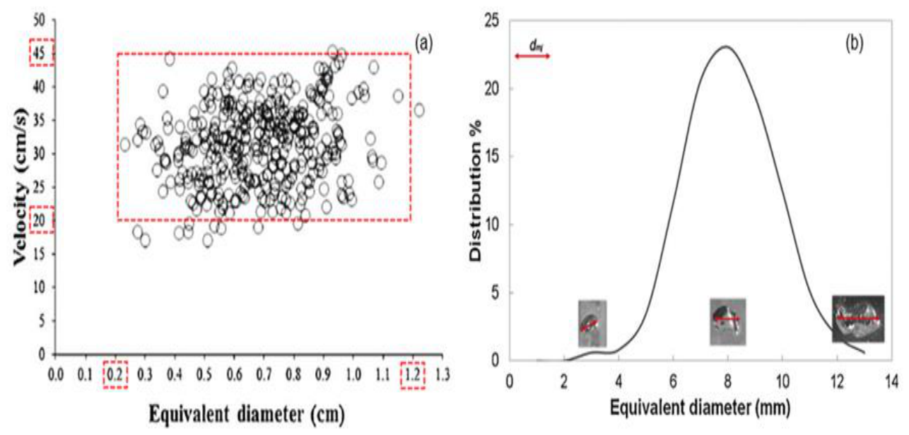
Data from the field experiment examining the dynamics of rising CO₂ bubble plumes, conducted as part of the QICS project in Scottish seawater, were used to validate the CFD methodology. The CFD simulations were validated against experimental data from controlled small-scale CO₂ releases, providing crucial insights into flow behavior. This validation is essential for environmental risk assessment and the development of predictive models for potential CCS leakage. Velocity profiles and bubble diameters were analyzed using simulation data, with black markers indicating laboratory experimental data. Figure 2 shows the simulated bubble diameters ranged from 0.20 to 1.20 cm, with the most frequent sizes between 0.50 and 0.90 cm, and the average rise velocity was 24–36 cm/s. These simulated values are consistent with experimental measurements from the QICS experiment. As shown in Figure 3, the QICS data indicate bubble diameters between 0.20 and 1.20 cm (with more than 50% of CO2 bubbles dimeter is between 0.65 and 0.9 cm) and velocities ranging from 20 to 45 cm/s, with approximately 75% of the bubbles rising at 25–40 cm/s [11].

3.2. Validation with the Huser Tank Experiment
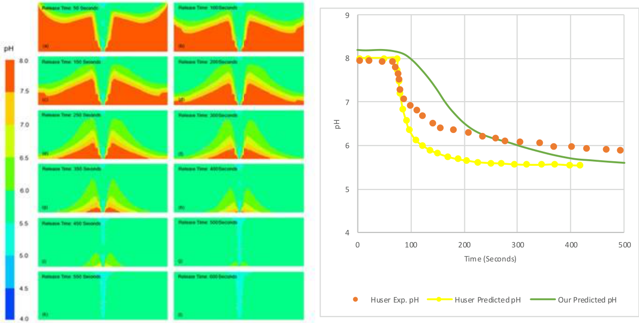
The primary objective of this study was to validate a numerical CFD model predicting the behavior of underwater CO₂ releases by comparing simulation results with experimental data from the Huser Tank experiments [15] conducted at the DNV GL Spadeadam facility. The comparison focused on pH variation and velocity characteristics during CO₂ dissolution in seawater. In the simulations, the release of CO₂ gas substantially altered the initial pH and pCO2​​ levels of the water. As the CO₂ bubbles dissolved, pCO2​​ increased due to chemical interaction with the water, while the pH decreased correspondingly. The simulations also show that the water's pH drops to a value of 5.6 in about 2-3 minutes that is in good agreement with the experimental observations showing the pH drops from 8.0 to 5.8 after 500 seconds.
Figure 4. (I) pH contour of bubble plume at release times from 50 to 600 seconds in 50-second intervals, shown in subfigures (a) to (l), respectively. (II) Comparison of measured and predicted pH. .
Preprints 221053 g004

3.3. Plume Dispersion Dynamics and Attenuation Height Estimation

In the event of a CO₂ leak from a ruptured undersea pipeline, estimating the attenuation height is essential. This height refers to the vertical distance required for the gas plume to disperse and reduce its concentration to a level that prevents it from escaping into the atmosphere. Accurate estimation is necessary because the rising gas plume generates turbulence that disrupts surrounding flow dynamics, reduces buoyancy in certain regions and creates variations in density, which can affect marine maneuverability in nearby shipping lanes.
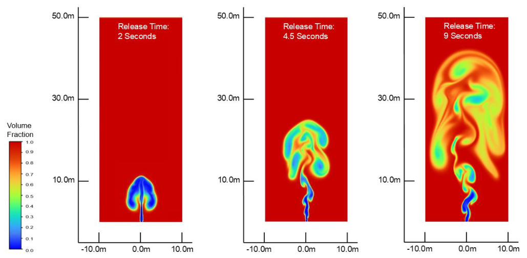
The simulation results for a major CO₂ leak (35 kg/s) provide critical insights into the plume’s behavior. Key variables measured include the plume’s height, width, and the time taken to reach the water’s surface. As shown in Figure 5, the plume reached its maximum height approximately 9 seconds after the initial blowout, demonstrating the rapid vertical ascent of the gas. Furthermore, the plume traveled 10 meters in less than 2 seconds and covered 20 meters in 4.5 seconds.

3.4. Jet-to-Buoyant Plume Transition

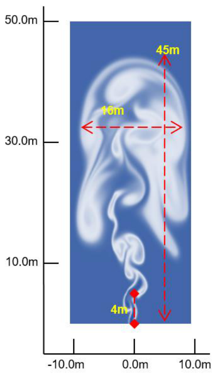
The gas is released as a jet for the first 4 meters and then transitions into a buoyant plume. The data shows that the plume will exceed the water column height present at High Island 10L site within 4.5 seconds. This emphasizes the gas plume's violent lateral release and its potential reach beyond the immediate leak area.
The volume fraction study provided important insights into the behavior of the gas-liquid system. High liquid flow velocities were observed in regions with a high gas volume fraction, while an increased liquid volume fraction appeared as the plume transitioned from a jet to a buoyant plume while rising, as shown in Figure 6.
Also, the variation in CO₂ volume fraction along the height of the water column was examined. The results show that between 4 m and 40 m, the CO₂ volume fraction decreases significantly, above 45 m, only a minimal amount of CO₂ remains. Accurate assessment of the potential impacts on marine ecosystems, nearby infrastructure, and human health depends on understanding the plume's extent.

3.5. Velocity and Pressure Distribution

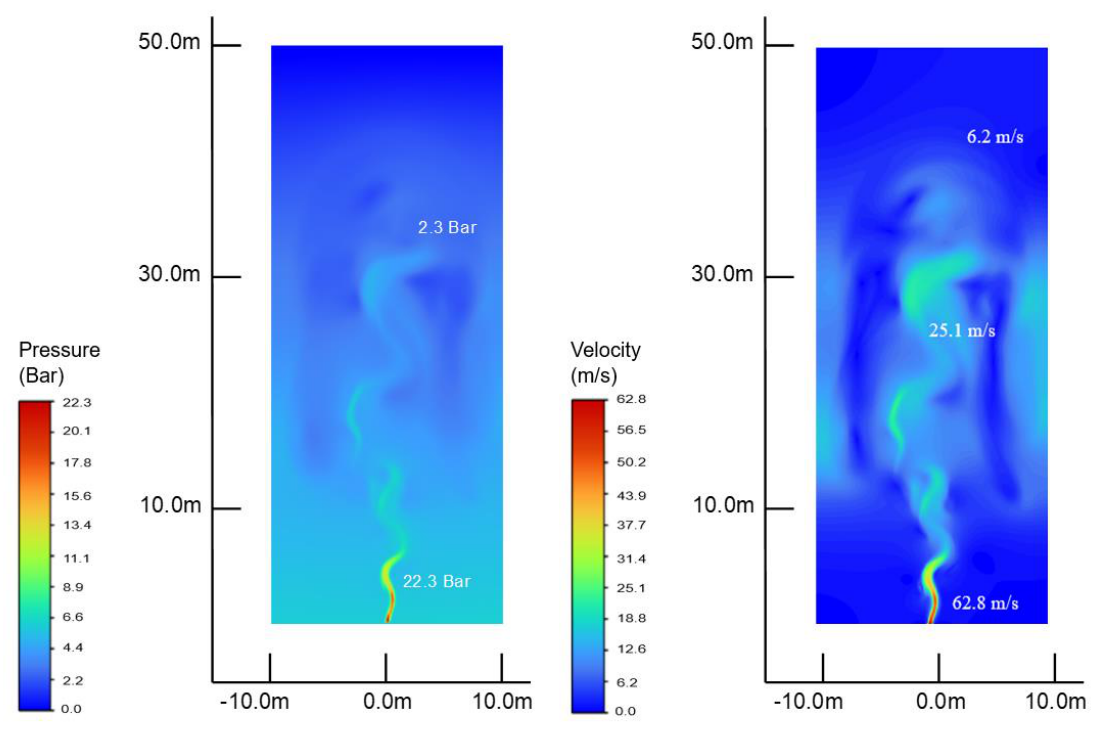
For this case, the plume rises to a height of 45 meters and expands laterally to a maximum width of 16 meters. As shown in Figure 7 (II), the CO₂ velocity at the leak source reaches 62.8 m/s. However, as the plume ascends through the water column, its velocity decreases significantly, with the lowest values measured near 40 meters, where it drops to a range of 0 to 6 m/s. A substantial drop in pressure is also observed as the plume rises. The pressure at the seabed is approximately 22.3 bar, remaining relatively high within the first 10 meters, but decreasing to around 2.3 bar at a height of 35 meters, as detailed in Figure 7 (I).

3.6. Prediction of p H and p C O 2

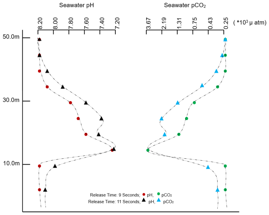
As shown in Figure 8, the seawater pH value dropped from 8.2 to 7.2. This decrease in pH indicates a rise in acidity as more CO2​ reacts with seawater. Concurrently, the rise in pCO2 from 0.254×10³ µ atm to 3.666×10³ µ atm confirms the buildup of CO2​ within the seawater. This change in pH can have adverse effects on the marine environment and the creatures that live there.

4. Discussion

4.1. Validation with the QICS Experiments

Figure 2 (I) presents the CFD results, illustrating the evolution of CO₂ bubble diameters over time. As previously discussed regarding bubble sizes, the visualizations emphasize general trends in bubble behavior. The increase in bubble size over time is primarily due to coalescence events, where smaller bubbles merge during plume ascent. In the upper regions at later times (15–20 seconds), a more dispersed bubble size distribution is observed, suggesting that breakup and mixing processes become more dominant as the plume interacts with the surrounding seawater. Overall, the figure demonstrates the dynamic behavior of bubble growth, coalescence, and dispersion over time, capturing the transition from a compact release zone to a more developed, turbulent CO₂ plume. In Figure 2 (II), As time progresses to 10 s and 15 s, the peak velocities decrease, and the plume core extends vertically while spreading laterally, indicating momentum diffusion and interaction with the surrounding fluid.

4.2. Validation with the Huser Tank Experiment

The pH evolution was monitored until the water reached equilibrium, and the CFD simulations reproduced this trend with excellent accuracy, reaching a saturated state after roughly 500 seconds (as shown in Figure 4). The model successfully captured the rapid initial mass transfer, followed by a slower rate as the solution approached saturation, resulting in a final pH of ~ 5.6.
Overall, the agreement between the simulated and experimental results validates the CFD model’s predictive capability. A slight discrepancy in the initial change in pH may be attributed to the higher carbonate concentration assumed in the simulation, as Huser's work did not specify the exact carbonate concentration

4.3. Subsea Bubble Plume

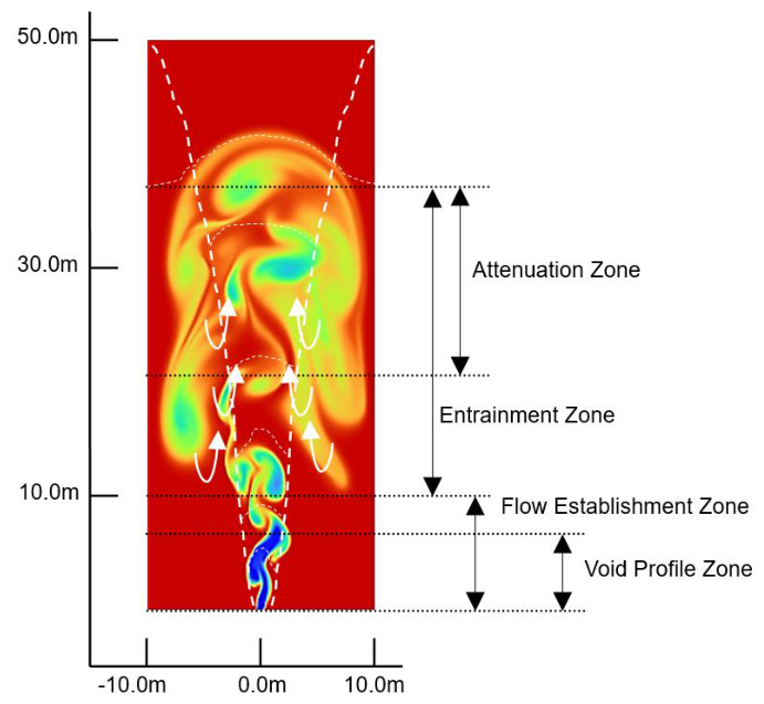
For analyzing the subsea bubble plume, the plume domain was divided into distinct zones that can be classified based on their characteristics and behavior. These zones include Attenuation, Entrainment, Flow establishment, and Void Profile zones. Each zone plays a significant role in the overall dynamics of the subsea bubble plume as delineated in Figure 9.
The flow is governed by the gas-liquid phase interaction in all these zones. The multiphase behavior results from the interfacial surface tension and the significant contrast in density and viscosity. The density ratio is responsible for the dominant driving force: buoyancy. Drag, turbulence, and gas dissolution govern the bubble plume. The following characteristics commonly describe the release point: release depth, release area, reservoir volume and pressure, gas rate, temperature, and gas composition. These properties vary for different release scenarios ranging from minor leaks from subsea equipment to enormous blowouts and pipeline ruptures. The zone above the release point is the gas Flow Establishment Zone, which is approximately up to 10m in case of 35 kg/s release. The gas can enter the liquid domain as a bubbling or gaseous jet depending on flow conditions in the constricting release area.
The gas will enter as a bubbling gas jet if the flow is not choked. If the flow is choked, the gas will enter as a gaseous jet. The penetration distance of the gaseous jet will further depend on whether the gas at the release area is fully expanded or under-expanded. In this case, if a pipe develops a leak and the pipe pressure is higher than the ambient pressure, the pressure in the constricting area of the release will be higher than the ambient pressure. Thus, the flow will go supersonic downstream of this constriction resulting in a complex pattern of shocks and oblique pressure waves. The gaseous jet will break into bubbles due to interfacial shear forces in the flow establishment zone. The breakup and mixing occur in the entrainment zone above which the gas will rise as bubbles. For most scenarios, this is the dominant zone. In this zone, the gas rises as dispersed bubbles due to buoyancy, and the momentum carried by the jet is insignificant compared to the momentum generated by the buoyancy of the gas. For a 50 m release scenario, the residence time of the gas bubbles is large enough for gas dissolution to be significant. This mass transfer phenomenon is governed by residence time, slip velocity, solubility, diffusivity, and surface area (i.e., bubble size). In the case of High Island 10L (10 – 20 m water depth), the gas dissolution will be minimal due to the jet behavior and will emerge at the surface. It is evident from the volume fraction and velocity contours that the surfaced gas will be of such quantities that the ocean will appear to boil, and a spout of water and gas will be present. Unlike the gas released upwards into the atmosphere, the entrained water cannot continue its upward motion when it reaches the surface. The rising water is diverted outward from the plume eye into a radial flow. This radial flow is potentially strong enough to affect surface vessels and cause capsizing.

4.4. Comparison with Oldenburg and Pan’s Work

In this section, a comprehensive comparison of our work with that of Oldenburg and Pan [4] is presented. Identical pipe leakage orifice diameter and flowrate (2 inches and 35.52 kg/s, respectively) were employed. Seawater chemical properties at the Gulf of Mexico and integrated kinetics of CO2 dissolution in seawater, a factor not considered in their research, are considered in this work. Furthermore, While Oldenburg and Pan utilized T2Well and TAMOC software, we employed Ansys Fluent to incorporate hydrodynamics and kinetics for CFD simulation, thus enriching the analysis and enhancing the understanding of the studied phenomenon. Moreover, the change in pH and pCO2 resulting from the CO2 release were modeled, providing a more comprehensive assessment of the environmental consequences of subsea CO2 leaks.
For the constant CO2 flow rate of 35 kg/s; the key differences lie in the velocity, transition length, and time to reach maximum height. The comparison is summarized in Table 2. In this study, the bubble plume reached a maximum height of 45 m in 9 seconds, while in Oldenburg's work, a shorter time of 5 seconds was observed. The disparity in time can be attributed to the consideration of reaction kinetics or equilibrium models in our research, which might have influenced the vertical motion of the CO2 plume. The lateral extent of the plume remains relatively consistent between these two studies.

5. Conclusions

In conclusion, this study considers the dependence of Henry's law constant on seawater salinity, CO₂ dissolution kinetics, and the mass transfer coefficient (estimated using the Hughmark correlation). The CFD model predicts hydrodynamic parameters such as plume velocity, rise time, transition length from jet to buoyant plume, height, and width, as well as kinetic parameters like pH and pCO2.
The CFD model was successfully validated using two rigorous CO2 release experimental data: the QICS and the Huser Tank Experiments. The QICS experiment aimed to simulate the behavior of CO2 bubbles when seepage from the sediments occurs. The simulation results (the bubble diameter from 0.2 to 1.2 cm and the average velocity between 24 and 36 cm/s) align with the experimental data observed (a bubble diameter ranging from 0.2 to 1.2 cm and a bubble velocity between 20 and 45 cm/s). The simulations also show that the water's pH drops to a value of 5.6 in about 2-3 minutes that is in good agreement with the experimental observations showing the pH drops from 8.0 to 5.8 after 500 seconds.
Subsequently the CFD model was used to predict a hypothetical pipeline blowout at 50 m water depth in the Gulf of Mexico as well as at 10 m depth similar to the High Island 10L site. The results of the 50m depth with a 35 kg/s release rate are compared with Oldenburg & Pan’s model predictions. Initially, the plume has a spherical cap shape, rising from the leaking point and gradually slowing down. Turbulence and lift forces cause the bubbles to spread out laterally, but they have little effect on the velocity of the bubbles. The CO2 plume reaches a maximum height of 45 meters with a width of 16 meters. The maximum pH change was observed at a height between 25 to 35 meters in the water column, where the lowest recorded pH value was 7.22. Furthermore, the simulations demonstrated a notable reduction in CO2 velocity as the plume crossed the 40-meter mark in the water column, with a 90% reduction observed. It is also worth noting that no significant pH changes were observed at heights below 10 meters. Furthermore, the comparison with Oldenburg's work for the 50m High Island case provided an additional means of assessing the CFD model's performance against an established benchmark. The agreement between the CFD results and Oldenburg's findings further confirmed the accuracy and reliability of the model, demonstrating its capability to reproduce the flow characteristics in a specific offshore scenario.
Even though the results of the CFD simulations help us understand how a large CO2 leak would behave, it is essential to note that more research, including experimental data validation and field observations, is needed to fully evaluate the effects on the environment and improve our understanding of how CO2 spreads in marine environments. Also, the model can be easily extended to atmospheric dispersion of released CO2 gas which is classified as an asphyxiant, displacing the oxygen in air.

Supplementary Materials

The following supporting information can be downloaded at Preprints.org.

Author Contributions

Conceptualization, Daniel Chen; Methodology, Daniel Chen and Napoli Rosario; Software, Napoli Rosario, Vinayak Rajan and Negar Hooshmand; Validation, Napoli Rosario, Vinayak Rajan; Formal analysis, Vinayak Rajan and Negar Hooshmand; Investigation, Napoli Rosario, Vinayak Rajan, Negar Hooshmand; Resources, Daniel Chen; Data curation, Napoli Rosario and Negar Hooshmand; Writing original draft preparation, Vinayak Rajan and Negar Hooshmand; writing—review and editing, Daniel Chen and Negar Hooshmand; Visualization, Napoli Rosario, Vinayak Rajan, Negar Hooshmand; Supervision, Daniel Chen; Project administration, Daniel Chen; Funding acquisition, Daniel Chen.

Funding

Financial support from “Offshore Gulf of Mexico Partnership for Carbon Storage--Resources and Technology Development,” Department of Energy Offshore Gulf of Mexico; # DE-FE0031558, LU Subaward UTA18-000644, 4/1/2018-3/31/2023 and Texas Louisiana Carbon Management Community, UTAUS-SUB00001635, USDOE NETL, DE-FE0032361, 2024-2028.are greatly acknowledged.

Acknowledgments

Special thanks are due to Curtis Oldenburg at the Lawrence Berkeley National Laboratory (LBL) for valuable discussions and Margaret A Murakami, Susan D. Horvoka, and Ramon H. Trevino at the University of Texas, Austin (UT) for providing marine environmental data near 10L and 24L lease blocks in Texas State Waters.

Conflicts of Interest

The authors declare no conflicts of interest.The funders had no role in the design of the study; in the collection, analyses, or interpretation of data; in the writing of the manuscript; or in the decision to publish the results.

Abbreviations

The following abbreviations are used in this manuscript:
CFD Computational Fluid Dynamics
QICS Quantifying and Monitoring Potential Ecosystem Impacts of Geological Carbon Storage
CCS Carbon Capture and Storage
DIC Dissolved Inorganic Carbon
SST Shear Stress Transport
TA Total Alkalinity
PBE Population Balance Equation

References

  1. Marchetti, C. ON GEOENGINEERING AND THE C02 PROBLEM. [PubMed]
  2. Olsen, J.E.; Skjetne, P. Current Understanding of Subsea Gas Release: A Review. Can. J. Chem. Eng. 2016, 94, 209–219. [Google Scholar] [CrossRef]
  3. Dewar, M.; Sellami, N.; Chen, B. Dynamics of Rising CO2 Bubble Plumes in the QICS Field Experiment. Int. J. Greenh. Gas. Control 2015, 38, 52–63. [Google Scholar] [CrossRef]
  4. Oldenburg, C.M.; Pan, L. Major CO2 Blowouts from Offshore Wells Are Strongly Attenuated in Water Deeper than 50 m. Greenh. Gases Sci. Technol. 2020, 10, 15–31. [Google Scholar] [CrossRef]
  5. Available online: https://Texasseagrant.Org/Wp-Content/Uploads/2025/06/15-405.
  6. Kano, Y.; Sato, T.; Kita, J.; Hirabayashi, S.; Tabeta, S. Model Prediction on the Rise of pCO2 in Uniform Flows by Leakage of CO2 Purposefully Stored under the Seabed. Int. J. Greenh. Gas. Control 2009, 3, 617–625. [Google Scholar] [CrossRef]
  7. Kano, Y.; Sato, T. Numerical Study on the Rise of pCO2 in Seawater by the Leakage of CO2 Purposefully Stored under the Seabed. Energy Procedia 2009, 1, 1909–1916. [Google Scholar] [CrossRef]
  8. Dewar, M.; Wei, W.; McNeil, D.; Chen, B. Simulation of the Near Field Physiochemical Impact of CO2 Leakage into Shallow Water in the North Sea. Energy Procedia 2013, 37, 3413–3423. [Google Scholar] [CrossRef]
  9. Dewar, M.; Wei, W.; McNeil, D.; Chen, B. Small-Scale Modelling of the Physiochemical Impacts of CO2 Leaked from Sub-Seabed Reservoirs or Pipelines within the North Sea and Surrounding Waters. Mar. Pollut. Bull. 2013, 73, 504–515. [Google Scholar] [CrossRef] [PubMed]
  10. Blackford, J.; Stahl, H.; Bull, J.M.; Bergès, B.J.P.; Cevatoglu, M.; Lichtschlag, A.; Connelly, D.; James, R.H.; Kita, J.; Long, D.; et al. Detection and Impacts of Leakage from Sub-Seafloor Deep Geological Carbon Dioxide Storage. Nat. Clim. Change 2014, 4, 1011–1016. [Google Scholar] [CrossRef]
  11. Sellami, N.; Dewar, M.; Stahl, H.; Chen, B. Dynamics of Rising CO2 Bubble Plumes in the QICS Field Experiment. Int. J. Greenh. Gas. Control 2015, 38, 44–51. [Google Scholar] [CrossRef]
  12. Shitashima, K.; Maeda, Y.; Sakamoto, A. Detection and Monitoring of Leaked CO2 through Sediment, Water Column and Atmosphere in a Sub-Seabed CCS Experiment. Int. J. Greenh. Gas. Control 2015, 38, 135–142. [Google Scholar] [CrossRef]
  13. Pham, L.H.H.P.; Rusli, R.; Shariff, A.M.; Khan, F. Dispersion of Carbon Dioxide Bubble Release from Shallow Subsea Carbon Dioxide Storage to Seawater. Cont. Shelf Res. 2020, 196. [Google Scholar] [CrossRef]
  14. Pham, L.H.H.P.; Rusli, R.; Shariff, A.M.; Khan, F. Dispersion of Carbon Dioxide Bubble Release from Shallow Subsea Carbon Dioxide Storage to Seawater. Cont. Shelf Res. 2020, 196, 104075. [Google Scholar] [CrossRef]
  15. Huser, A.; Vollestad, A.; Rivedal, N. Accidental Underwater Release of CO 2 —CFD Modelling of the Underwater Plume and the Subsequent above Water Gas Dispersion; 2016; pp. 1526–1532. ISBN 978-1-138-02997-2. [Google Scholar]
  16. Wilcox, D.C. Turbulence Modeling for CFD; DCW industries La Canada, CA, 1998; Vol. 2. [Google Scholar]
  17. Fluent Theory Guide. Available online: https://ansyshelp.ansys.com/public/account/secured?returnurl=/Views/Secured/corp/v242/en/flu_th/flu_th.html (accessed on 9 January 2026).
  18. Launder, B.E.; Spalding, D.B. The Numerical Computation of Turbulent Flows. Comput. Methods Appl. Mech. Eng. 1974, 3, 269–289. [Google Scholar] [CrossRef]
  19. Olsen, J.E.; Dunnebier, D.; Davies, E.; Skjetne, P.; Morud, J. Mass Transfer between Bubbles and Seawater. Chem. Eng. Sci. 2017, 161, 308–315. [Google Scholar] [CrossRef]
  20. Glade, H.; Al-Rawajfeh, A.E. Modeling of CO2 Release and the Carbonate System in Multiple-Effect Distillers. Desalination 2008, 222, 605–625. [Google Scholar] [CrossRef]
  21. Plummer, L.N.; Busenberg, E. The Solubilities of Calcite, Aragonite and Vaterite in CO2-H2O Solutions between 0 and 90°C, and an Evaluation of the Aqueous Model for the System CaCO3-CO2-H2O. Geochim. Et. Cosmochim. Acta 1982, 46, 1011–1040. [Google Scholar] [CrossRef]
  22. Danckwerts, P.V. Gas-Liquid Reactions; 1970. [Google Scholar]
  23. Narsimhan, G.; Gupta, J.P.; Ramkrishna, D. A Model for Transitional Breakage Probability of Droplets in Agitated Lean Liquid-Liquid Dispersions. Chem. Eng. Sci. 1979, 34, 257–265. [Google Scholar] [CrossRef]
  24. Luo, H. Coalescence, Breakup and Liquid Circulation in Bubble Column Reactors.; Norges Tekniske Hoegskole: Trondheim., 1993. [Google Scholar]
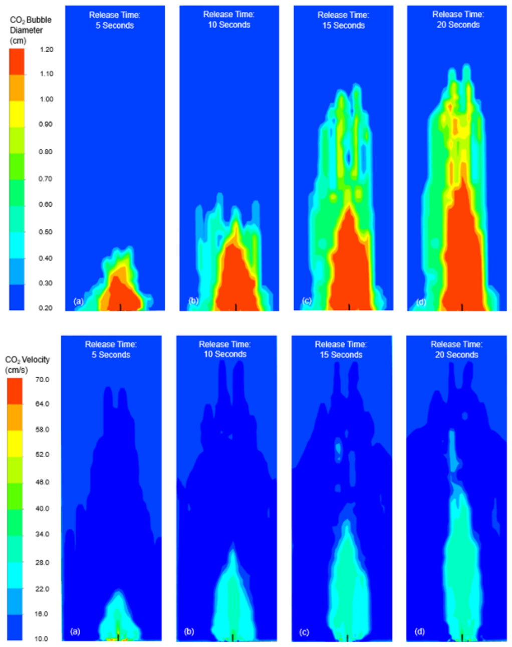
Figure 2. (I) CO2 Bubble diameter Contour at release time (a) 5 seconds, (b) 10 seconds, (c) 15seconds and (d) 20 seconds (II) Velocity Contour of Bubble Plume at release time (a) 5 seconds, (b) 10 seconds, (c) 15seconds and (d) 20 seconds.
Preprints 221053 g002
Figure 3. (a) Velocity vs. Equivalent Diameter, (b) Distribution (%) vs. Equivalent Diameter (mm) at 9–12 m water depth [11].
Preprints 221053 g003
Figure 5. Volume fraction contours of the plume at sequential release times: (a) 2 s, (b) 4.5 s, and (c) 9 s.
Preprints 221053 g005
Figure 6. Plume Spread across the domain.
Preprints 221053 g006
Figure 7. (I) Pressure (L) Contours and (II) Velocity (R) Contours.
Preprints 221053 g007
Figure 8. pH and pCO2 profiles at various depths.
Preprints 221053 g008
Figure 9. Bubble Plume Zone’s. .
Preprints 221053 g009
Table 2. Comparison with Oldenburg & Pan’s work.
Parameters Oldenburg & Pan Our study
CO2 Leakage Flowrate 35.52 kg/s 35 kg/s
Orifice Diameter 2’’ 2’’
Velocity 52.29 m/s 62.8 m/s
Length scale, Jet to plume 2.2 m 4-10 m
Time (Leak Point to 50m) 5 s 7-9 s
Time (Leak Point to 10m) < 1 s < 2 s
Bubble Diameter 5.075 ×10⁻⁴ m (avg.) 5.0 ×10⁻⁴ m (fixed)
Plume Diameter (50m case) 15 m 16 m
Plume Diameter (10m case) 3.2 m 4-5 m
Attenuation Height 50 m 45-50 m
Depth 50 m 50 m
Disclaimer/Publisher’s Note: The statements, opinions and data contained in all publications are solely those of the individual author(s) and contributor(s) and not of MDPI and/or the editor(s). MDPI and/or the editor(s) disclaim responsibility for any injury to people or property resulting from any ideas, methods, instructions or products referred to in the content.
Copyright: This open access article is published under a Creative Commons CC BY 4.0 license, which permit the free download, distribution, and reuse, provided that the author and preprint are cited in any reuse.
Prerpints.org logo

Preprints.org is a free preprint server supported by MDPI in Basel, Switzerland.

Subscribe

© 2026 MDPI (Basel, Switzerland) unless otherwise stated

Accessibility

Disclaimer

Terms of Use

Privacy Policy

Privacy Settings