
Submitted:
30 June 2026
Posted:
01 July 2026
You are already at the latest version
Abstract
Time-reversed Young (TRY) interferometry reconstructs interference from a fixed detector by reading out a programmable source-label distribution. We formulate this architecture as a source-coded Bayesian response sensor. For a perturbation parameter θ, the detected source-label histogram is a posterior distribution determined by a programmed source prior, an optical likelihood for a fixed-detector click, and an evidence factor equal to the click probability. The key point is not the Bayesian identity itself, but its physical implementation: in TRY the prior is imposed before propagation and can therefore reshape the response ensemble actually sampled by the detector. We show that the normalized posterior responds through a centered likelihood score, and that the detected-event Fisher information is the posterior variance of this score. This identifies posterior-weighted score contrast, rather than local response magnitude alone, as the relevant sensing resource. The framework separates posterior-shape information from evidence information, giving a resource-aware way to judge near-null response enhancement. It also yields practical design rules: a two-label source code converts a weak perturbation into a fixed-detector label imbalance, while the multiparameter score covariance provides a route to nuisance rejection and gives a minimal-label rank condition for sensing multiple perturbations. A passive double-slit implementation with weak one-slit phase and loss perturbations is proposed, requiring only fixed-detector source scans before and after calibrated perturbations. The results position TRY as a source-programmable Bayesian sensing architecture complementary to conventional detector-plane Young interferometry.
Keywords:
time-reversed Young interferometry
; Bayesian optical sensing
; source-prior engineering
; Fisher information
; optical interferometry
; fixed-detector sensing
; source coding
1. Introduction
Young’s double-slit experiment is normally a predictive measurement. A known source prepares an optical field, and interference is observed as a detector-plane intensity distribution. In its simplest form, a fixed source coordinate produces a normalized response over detector coordinate x. By contrast, time-reversed Young (TRY) interferometry changes this statistical arrangement. A detector is fixed at coordinate d, while a point-addressable source coordinate y is scanned or programmed. The interference pattern is then reconstructed in source-label space rather than by scanning the detector plane [1,2,3].
This reversal is more than a geometric relabeling. In conventional Young interferometry (CYI), the detector coordinate is the output random variable. In TRY, the detected event at d conditions the source-label distribution. Thus the measured object is naturally a posterior distributionn [4,5,6],
where is the programmed source prior, is the likelihood for a click at the fixed detector, and denotes a physical perturbation inside the interferometer. The normalization
is the evidence. Experimentally, Z is also the click probability for the chosen source program [5,6].
The appearance of Bayes’ rule is not itself the novelty. Bayesian inference, score functions, Fisher information, and weak-response formulas are standard tools in estimation theory and optical metrology [7,8,9,10,11,12]. The point here is that TRY gives these tools a distinct physical implementation. The prior is not a post-processing weight applied after detection; it is imposed before propagation through the source dwell time, source brightness, an addressable emitter array, a digital micromirror device, or a spatial light modulator. Changing changes the ensemble of source labels that actually contributes to fixed-detector clicks. This makes the source plane a programmable statistical resource.
Such a source-programmed fixed-detector viewpoint is conceptually adjacent to coded-aperture imaging, Hadamard-transform optics, single-pixel compressive imaging, and computational ghost imaging, where spatial or statistical information is transferred from detector arrays to programmed illumination or source patterns [13,14,15,16]. But in TRY the programmed variable is the source-label prior entering a fixed-detector posterior rather than an object mask or detector-side postselection [17,18,19,20].
Figure 1 summarizes this architecture. A programmed source prior prepares the source-label ensemble before propagation through a passive Young aperture. For a fixed detector coordinate d, the optical system defines the likelihood , while the detected data separate into the posterior shape and the evidence . This diagram also clarifies the operational difference from CYI: TRY moves the programmable degree of freedom to the source side and leaves the detector fixed [21,22].
The central question addressed in this work is therefore not whether TRY obeys a Bayesian identity, but whether the Bayesian structure can be used to engineer optical response. Given a weak perturbation such as a one-slit phase shift, one-slit loss, tilt, defocus, or local refractive-index change [2,3,23], we ask how the detected source-label posterior moves and how this motion can be optimized by source programming. The answer is that TRY sensitivity is governed by the posterior variance of the perturbation score [6,7,8]. Consequently, the useful resource is not the largest local response at a single source label, but the posterior-weighted contrast among source labels with different responses.
This distinction has practical consequences. It separates normalized posterior-shape information from evidence, or rate, information [5,6]. It leads to a two-label differential source code that converts a weak perturbation into a fixed-detector source-label imbalance. It also gives a multiparameter covariance rule for choosing source labels that enhance a target perturbation while suppressing nuisance parameters [8,9,24]. These results do not imply that TRY universally outperforms CYI. Rather, the two settings define different statistical experiments: conventional Young samples detector-coordinate scores from a fixed source, whereas TRY samples source-label scores conditioned on a fixed detector and shaped by a programmable prior.
The paper is organized as follows. Section 2 defines the CYI and TRY statistical experiments. Section 3 derives the TRY susceptibility and its Fisher information. Section 4 develops the statistical consequences: shape–evidence separation, differential source coding, multiparameter covariance, nuisance rejection, and a minimal-label rank rule. Section 5 gives a passive double-slit realization. Section 6 presents an experimental protocol and a conventional Young control. Section 7 discusses physical meaning, limitations, and complementarity. Detailed algebra that is standard but useful for checking is placed in the Appendices.
2. Optical Model and Statistical Experiments
2.1. Passive Scalar Propagation
We consider a one-dimensional scalar paraxial model. The source coordinate is y, the aperture coordinate is , and the detector coordinate is x. Propagation from the source plane to the aperture plane is described by , the aperture by T, and propagation from the aperture plane to the detector plane by . A physical perturbation is denoted by . It may represent, for example, a one-slit phase shift, one-slit loss, transverse tilt, defocus, or a local refractive-index change [2,3,25,26].
The transition amplitude from source coordinate y to detector coordinate x is
Equivalently, in an intermediate-plane representation,
where and are the source-to-aperture and aperture-to-detector propagation kernels. Such kernel representations are standard in scalar diffraction theory and in paraxial optical-system propagation [2,3,27]. For free-space paraxial propagation over distance z,
with wavelength and wavenumber . This is the one-dimensional Fresnel propagator used throughout the paraxial approximation [2,3,27].
The ideal likelihood for detecting a photon, or an optical count, at x given source label y is proportional to . In an experiment, one may include known throughput and background terms:
Here describes calibrated source and detector efficiency, and is background. This form follows the usual intensity-detection model, with calibrated efficiency and additive background treated separately from coherent propagation [25,26,28]. The theoretical derivations use the ideal limit and slowly varying for clarity. The count-ratio estimators in Sec. Section 6 include background subtraction explicitly.
The same optical likelihood underlies CYI and TRY. The distinction between the two settings is statistical: which coordinate is fixed, which coordinate is observed, and which coordinate can be programmed before detection. This distinction is the point at which the present work departs from standard propagation theory and defines a different statistical experiment [21,22,29,30,31,32,33,34,35].
2.2. Conventional Young Statistical Experiment
In CYI, the source coordinate is fixed at , and the detector coordinate x is the observed random variable. The normalized detector-plane distribution is
For a perturbation , the detector-coordinate score is
The detector-shape Fisher information is therefore
Equation (9) is the typical score-variance form of Fisher information [7,8,9]. It is included to make the comparison precise: CYI can be analyzed by the same score-variance language, but the variance is taken over detector coordinate x, while the source coordinate is fixed.
2.3. TRY Posterior Statistical Experiment
In TRY, the detector coordinate is fixed at d, and the source coordinate is programmed according to , with . The detected source-label distribution is the posterior in Equation (1). For a discrete source basis , the prior is a set of programmed weights , and the posterior becomes
Experimentally, is estimated by the normalized fixed-detector count histogram over source labels. This is the discrete experimental form of the Bayesian update, with source-label weights playing the role of a physically programmed prior [4,5,6,21].
This is where TRY differs operationally from CYI. In CYI, x is an output coordinate generated by the optical field. In TRY, y is an input label selected before propagation. Therefore is a physical control variable. Changing changes which source labels contribute to the detected ensemble, rather than merely reweighting data after measurement. This pre-detection control is the statistical resource used in the susceptibility and source-code design developed below.
3. Bayesian Susceptibility and Fisher Information
We now ask how the TRY posterior responds to a weak physical perturbation. Let
be the likelihood score for source label y at fixed detector coordinate d. The score measures the fractional response of the optical likelihood to the perturbation, as in standard likelihood-based estimation theory [7,8,24].
The TRY susceptibility is defined as the logarithmic response of the normalized source-label posterior,
Using Equation (1), and assuming that the programmed prior is independent of the perturbation, one obtains
where denotes averaging over the detected posterior. The derivation is given in Appendix A.
Equation (13) is a standard centered-score identity for a normalized parametric distribution, but its physical meaning in TRY is important. The normalized posterior does not respond to the absolute likelihood score at one source label. It responds to the difference between that local score and the evidence-averaged score. A perturbation that multiplies all likelihoods by the same fractional factor changes the total click rate but leaves the normalized posterior shape unchanged.
The detected-event Fisher information carried by the posterior shape is
Thus the sensitivity of the normalized TRY source-label distribution is governed by the posterior variance of the perturbation score, the usual Fisher-information form for a normalized measurement distribution [7,8,9]. Useful posterior-shape sensing requires score heterogeneity across the detected source ensemble. A single source label, even one with a large local score, carries no shape information by itself. Conversely, two or more source labels with different scores can yield a strong posterior response, provided that they retain sufficient posterior weight.
This distinction is especially important near destructive interference. In many two-path settings, a local score can become large near a null because the total amplitude is small. Similar near-null response enhancement is familiar from weak-value and postselected metrology, where large conditional responses must be weighed against postselection probability and technical noise [10,11,12,36,37]. However, the same null can suppress the likelihood and hence reduce the evidence. The useful operating point is therefore not necessarily the darkest fringe. It is the region where the score contrast and detected posterior weight jointly maximize Equation (14), subject to the throughput constraints discussed below. Related optical-sensor implementations of weak-response amplification have appeared in weak-measurement-based biosensing and chiral sensing, although the present TRY mechanism uses source-prior engineering rather than detector-side postselection [38,39].
Figure 2 makes this tradeoff explicit for the balanced double-slit TRY model. Panel (a) shows the fixed-detector likelihood , which gives the source-space fringe sampled by the programmed source labels. is the relative phase between the lower and upper optical pathways and is defined in Equation (29). Panel (b) shows the corresponding posterior for a uniform source prior over the displayed phase interval; in this ideal case it has the same fringe shape as the likelihood, but normalized as a detected-event distribution. Panel (c) shows the one-slit phase score , whose magnitude increases near the source-space nulls because a small phase perturbation strongly changes the relative two-path cancellation. Panel (d) plots the information density , which remains finite because the posterior weight decreases where the local score grows. Thus the useful sensing region is not identified by the largest local score alone; it is identified by the overlap between appreciable detected probability and large centered-score contrast. This is the same statistical caution underlying Fisher-information analyses of amplified or postselected measurements, but here the conditional ensemble is engineered through the source prior rather than through detector-side postselection [21,36,37].
4. Statistical Consequences of the TRY Posterior
The posterior form of TRY has consequences beyond the statement that the source prior is programmable. It changes how perturbation information is organized. In CYI, one usually analyzes a detector-plane distribution generated by a fixed source. In TRY, the detected event defines a posterior ensemble of source labels. This posterior ensemble has a shape, an evidence, and a programmable support. These three features lead to useful statistical design rules [5,6,8,24].
4.1. Posterior-Shape Information and Evidence Information
The susceptibility in Equation (13) describes the response of the normalized posterior shape. Because it is a centered score, it is insensitive to a perturbation that multiplies all source-label likelihoods by the same fractional factor. Such a perturbation does not reshape the detected source-label histogram. It only changes the total probability of obtaining a fixed-detector click. This is the usual distinction between normalized distributional information and rate, or yield, information in likelihood-based measurements [8,24,36,37].
The latter effect is carried by the evidence. Its logarithmic response is
Thus, TRY naturally separates perturbation information into posterior-shape information and evidence, or rate, information. If total intensity is normalized away to reject source-power drift, detector-gain drift, or slow coupling fluctuations, then only the posterior-shape channel is retained. If the absolute click rate is stable and calibrated, the evidence can be used as an additional signal. This separation is also standard in experimental design, where one distinguishes information in the conditional distribution from information in event probability or acquisition rate [5,6].
For a discrete source program, a single source trial either produces a fixed-detector click with recorded label j, or produces no click. The per-trial Fisher information is
Its derivation is given in Appendix B. The first term is the click-probability-weighted information contained in the normalized posterior shape. The second term is the information carried by the total click/no-click rate. The same decomposition underlies Fisher-information analyses of postselected or lossy measurements, where conditional sensitivity must be assessed together with success probability [36,37,40].
When the rate channel is deliberately discarded, or when it is too noisy to be trusted, the relevant resource-aware shape metric is
This quantity prevents a common overinterpretation of near-null response enhancement. Near destructive interference, a local score may become very large, but the likelihood and hence the click probability may become very small. A large conditional response is experimentally valuable only if enough detected events remain to estimate it. This is the practical reason for reporting both conditional Fisher information and throughput-weighted information.
4.2. Differential Source Coding
The simplest nontrivial TRY source code uses two source labels, and . Let their detected posterior weights be and , and let their perturbation scores be and . The detected-event Fisher information then reduces to
This expression makes the role of score heterogeneity explicit. A single high-response label is not enough. The posterior must contain at least two labels whose scores are different. For fixed scores, Equation (18) is maximized by balanced detected posterior weights, giving
This is a standard variance result, but in TRY it becomes an optical design rule: choose source labels with large perturbation-score separation, then program the source prior so that both labels contribute comparably to the detected posterior. This is closely related in spirit to optimal experimental design, where measurement settings are chosen to maximize an information criterion rather than sampled passively [6,41,42,43].
If the two labels have likelihoods and , balanced detected posterior weights are obtained by
For a two-label-only program, the resulting evidence is
Equation (21) displays the throughput cost of balancing the posterior. It is the TRY version of a familiar design tradeoff: information can be concentrated in selected outcomes, but the acquisition probability of those outcomes remains part of the experimental resource budget [5,36,37]. That is, if one label lies near a null, its score may be large, but its likelihood is small. It must then be assigned a larger prior weight, or longer dwell time, to appear with comparable frequency among detected events.
Figure 3 illustrates the full two-label design logic. Panel (a) shows the fixed-detector likelihood landscape , from which two source labels and are selected. The labels need not have equal likelihoods; in fact, one may eliberately choose a lower-likelihood label if it provides a stronger perturbation response. Panel (b) shows the corresponding phase-score landscape , where the same two labels are chosen to produce a large score difference . Panel (c) then shows the essential source-prior correction: unequal programmed weights and compensate unequal likelihoods so that the detected posterior weights become balanced, . Panel (d) shows the resulting differential readout, where a weak one-slit phase perturbation is converted into a label imbalance D. Thus Figure 3 turns Equations (20) and (21) into an operational protocol: select labels by score contrast, balance them by dwell time, and estimate the perturbation from a fixed-detector count ratio. Unlike detector-side postselection, this balancing is imposed before propagation by changing the source dwell times.
With detected counts and , define the label imbalance
To first order in the perturbation,
At balanced detected posterior weights, . Thus the perturbation is converted into a fixed-detector source-label imbalance. Because D is a ratio, common detector gain fluctuations, acquisition-time fluctuations, and source-power drifts that affect both labels similarly are partially canceled. Such differential normalization is a standard strategy for suppressing common-mode technical noise in optical sensing and precision measurement [45,46].
The two-label code is therefore more than a minimal Fisher-information example. It is a practical fixed-detector differential sensor. A preliminary scan identifies candidate labels with large score separation and acceptable likelihood. A second measurement uses only those labels, with dwell times chosen from Equation (20). The perturbation is then estimated from the imbalance D, rather than from a full source scan.
4.3. Multiparameter Score Covariance and Nuisance Rejection
The same posterior-score structure extends directly to multiple perturbations. Let and define
The posterior-shape Fisher matrix is the score covariance,
This is the standard Fisher-information matrix for a multiparameter likelihood model [7,8,9,24]. Each source label carries a response vector . A source program selects which response vectors are represented in the detected posterior. Source-prior engineering is therefore equivalent to shaping the cloud of detected score vectors. This covariance view also connects the TRY Fisher matrix to the information-geometric interpretation of statistical models, where local distinguishability is encoded by the Fisher metric [44]. This gives a geometrical interpretation of source-code design analogous to information-matrix design in multiparameter estimation [9,42].
Figure 4 visualizes this covariance design principle for a two-parameter example. Panel (a) shows the target phase score across source-label phase coordinate , while panel (b) shows the nuisance loss score for the same labels. The red points mark three selected source labels, which sample the two score landscapes differently. Panel (c) replots the same selected labels as score vectors ; this representation makes the Fisher matrix geometrical, because is the posterior covariance of this score cloud. Panel (d) shows the resulting target information, cross covariance, and nuisance-eliminated information. The purpose is not merely to maximize the spread of , but to choose labels whose score vectors keep the target direction distinguishable from the nuisance direction. This distinction is important because large single-parameter information can still lead to poor usable sensitivity if it is strongly correlated with nuisance responses.
This is especially useful when one parameter is the desired signal and another is a nuisance. For a target parameter and a nuisance parameter , the information remaining after eliminating the nuisance is
A good source code should produce a large target-score variance while reducing covariance with nuisance scores. The same Schur-complement form appears in multiparameter estimation when nuisance parameters are eliminated from the Fisher matrix [8,9,24]. In practical terms, this means choosing source labels for which the desired perturbation changes the posterior shape in a direction distinguishable from loss, source-power drift, tilt, defocus, or other unwanted changes.
If the posterior occupies J source labels, the centered score covariance has rank at most :
Therefore, posterior-shape sensing of m independent parameters requires at least occupied source labels. One label gives no shape information. Two labels can sense only one independent perturbation direction. Three labels are the minimum for two independent directions. This rank statement is a discrete measurement-design constraint rather than a property of the optical aperture itself. This rule is simple but practically important: few-label TRY sensing is possible, but the number of occupied labels limits the number of independent perturbations that can be distinguished from posterior shape alone.
4.4. Statistical Complementarity with CYI
The statistical distinction between TRY and CYI is now sharper. CYI also has a score-variance description, but it samples a detector-coordinate score landscape generated by a fixed source. TRY samples a source-label score landscape conditioned on a fixed detector event and shaped by a programmable prior. This is consistent with the source-space reconstruction viewpoint of TRY [21], but here it is expressed as a comparison of statistical experiments rather than as a propagation symmetry.
These two landscapes need not carry the same perturbation information. A perturbation may produce a nearly constant detector-coordinate score in a CYI measurement, while producing strong score contrast across source labels in TRY. The reverse can also occur. The comparison is therefore not a universal sensitivity ranking. It is a comparison between two statistical projections of the same passive optical kernel. This avoids the common pitfall of comparing only local amplification factors without accounting for sampling probability, noise, and measurement architecture [36,37,40].
This complementarity is useful. CYI is naturally suited to detector-plane predictive sensing. TRY is naturally suited to source-posterior response sensing. Its distinctive advantage is that the source side can be programmed before detection. This enables posterior-shape design, differential source coding, and source-side nuisance rejection with a fixed detector. In applications where detector scanning, detector arrays, or detector flat-field calibration are costly or unstable, this source-side architecture can provide a practical alternative. The relevant performance comparison is therefore architecture-dependent and should include throughput, calibration stability, and available source-side programmability. This emphasis on a physically meaningful sensitivity metric is consistent with recent optical-sensing work that formulates sensor performance through information-theoretic or physics-based figures of merit [47].
5. Double-Slit Realization
We now specialize the general Bayesian response theory to a passive double-slit system. This case is analytically transparent and gives a direct experimental test of the proposed source-prior engineering protocol. This case also connects the present framework to the standard two-path interference model while allowing the response quantities to be written in closed form [1,2,3,28].
5.1. Two-Path TRY Likelihood
Consider two narrow slits at , with equal transmission amplitudes. The source-to-slit and slit-to-detector distances are and , respectively. Ignoring common prefactors that cancel in normalized probabilities, the two path amplitudes are
The use of two narrow-path amplitudes is the usual point-aperture limit of scalar diffraction theory [2,3,25]. At a fixed detector coordinate d, the TRY amplitude is . The relative phase between the lower and upper paths is
The resulting relative phase has the same linear source–detector structure as the ordinary double-slit phase, but here it is read by varying the source coordinate at fixed detector position. The fixed-detector likelihood is
Equation (30) is the source-space TRY fringe. This is the basic source-space reconstruction feature of TRY [21,22]. The detector is not scanned; the interference is observed by changing the source label y. The fixed detector coordinate d shifts the phase origin, while the source coordinate scans the phase.
This model is intentionally ideal. In an experiment, unequal slit transmission, finite slit width, background, and imperfect coherence modify the likelihood envelope and reduce the fringe contrast. But these effects do not change the Bayesian structure. They simply replace Equation (30) by the calibrated likelihood measured in the baseline source scan. Such corrections are standard in real interferometers and are naturally absorbed into the calibrated likelihood used by the Bayesian response analysis [26,28].
5.2. Weak One-Slit Phase Perturbation
Apply a weak phase to the upper slit,
One-path phase perturbations are the standard local probe in interferometric phase sensing [45,46]. Define the upper-path complex weight
Quantities of this form are closely related to local weak values and conditional path amplitudes, where a path projector is normalized by the total postselected amplitude [10,11,12,48,49]. The likelihood score for the phase perturbation is
as derived in Appendix D. Here the phase score is the imaginary part of the conditional path weight, consistent with the usual role of imaginary weak values as shifts in the conjugate response variable [11,12,50]. For the balanced two-slit model,
and therefore
Near a source-space dark point, with ,
This sensitivity–probability tradeoff is the same caution that appears in weak-value amplification and near-dark-port interferometry [36,37,40,51]. Equation (36) imply that the local score is enhanced as the null is approached, but the likelihood decreases quadratically. Hence the best sensing region is not the exact null. It is a region near the null where the score is large while the detected posterior weight remains sufficient.
5.3. Weak One-Slit Loss Perturbation
Apply instead a weak amplitude loss to the upper slit,
Amplitude loss provides the complementary perturbation to phase because it probes the in-phase, or real, component of the conditional path response. The corresponding likelihood score is
Together with the phase score, this gives an operational decomposition of the complex path weight into quadrature responses. Combining the phase and loss scores gives
Thus two calibrated perturbations, a phase perturbation and a loss perturbation applied to the same slit, reconstruct the complex upper-path response in source-label space. This is conceptually related to direct optical wavefunction and weak-value reconstruction, but the present object is a source-label-dependent response weight used for fixed-detector TRY sensing rather than a full quantum-state reconstruction [48,49,52].
Figure 5 shows how this reconstruction works in a slightly imbalanced two-path model. Panel (a) gives the fixed-detector likelihood , where the imbalance parameter prevents the nulls from becoming perfectly dark. Panel (b) shows the phase score , which probes the imaginary part of the upper-path weight and is strongly enhanced near the source-space destructive-interference points. Panel (c) shows the loss score , which probes the real part of the same path weight and becomes source-label dependent when . Panel (d) combines the two scores into the complex trajectory . Thus the figure gives a direct diagnostic test: agreement between the measured phase–loss reconstruction and the predicted trajectory verifies the two-path response model, while deviations reveal imbalance, finite-aperture effects, partial coherence, or background. This makes the figure a calibration diagnostic as well as a theoretical response plot.
In the perfectly balanced ideal model, , so the loss score is spatially constant and carries no normalized-shape information after centering. This does not make the loss scan useless. It contributes to the evidence channel, and in realistic systems with imbalance, finite slit width, partial coherence, or background, need not be constant. The loss scan then supplies the real part of the source-space path weight and helps diagnose path imbalance. This role is especially useful in realistic interferometers, where contrast and imbalance are often limited by unequal transmission and partial coherence [26,28].
Figure 5 should be used as the model-to-experiment bridge. It compares the analytic response expected from the calibrated geometry with the measured phase and loss score profiles obtained from the protocol below.
5.4. Relation to CYI in the Same Double-Slit System
For the same aperture, CYI with fixed source has detector-plane phase
and detector-plane likelihood
The local phase score has the same functional form,
This confirms that the local weak-response formula is not unique to TRY. The same tangent response is the ordinary two-path phase sensitivity near a dark fringe [2,3,45].
The difference is statistical and operational. CYI samples the score landscape by observing detector coordinate x for a fixed source . TRY samples the score landscape by programming source coordinate y for a fixed detector d. In the ideal symmetric double-slit model these landscapes are related by coordinate exchange, but in practical sensing the available controls are different. TRY allows the source prior to be designed before detection, enabling two-label source coding, posterior balancing, and fixed-detector differential readout. This is the point where TRY differs from both conventional detector-plane sampling and detector-side postselection: the informative ensemble is shaped by source programming before propagation. CYI would require detector scanning, detector-pixel weighting, or detector-side postselection to implement an analogous strategy. The distinction is therefore architectural rather than a claim that the local two-path response formula itself is new.
6. Experimental Protocol
The theory above can be tested with a passive double-slit setup and a fixed detector. The essential measurement is simple: record the source-label count histogram before and after a calibrated weak perturbation, then form the score, susceptibility, and Fisher information from count ratios. This section gives a minimal TRY protocol and a CYI control.
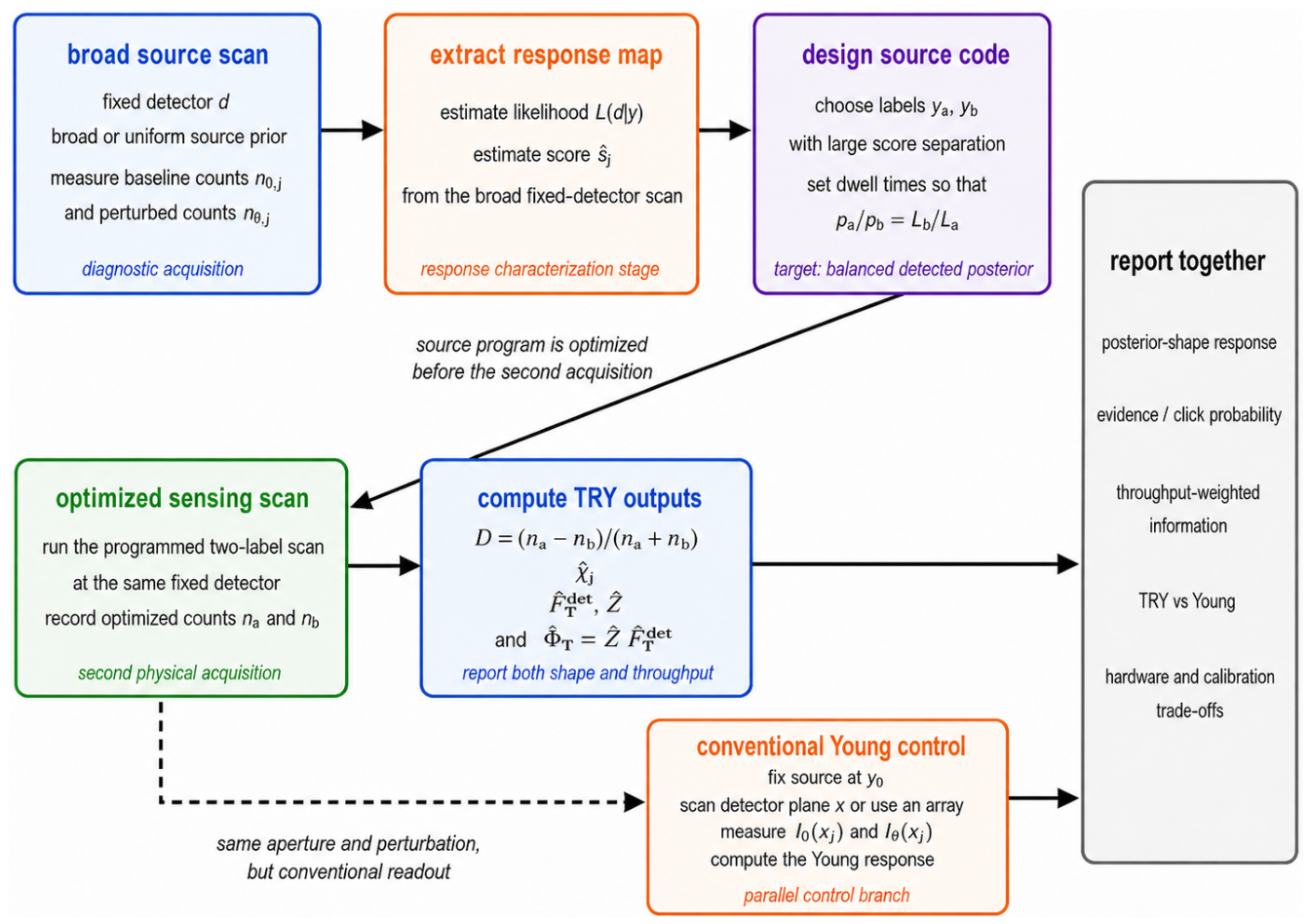
Figure 6 summarizes the experimental workflow. The first stage is a broad fixed-detector source scan, in which a uniform or broad source prior records baseline and perturbed count histograms over source labels. These data are used to estimate the likelihood landscape and the perturbation score , which are the empirical inputs to the Bayesian design rules derived above. The second stage uses these response maps to choose a source code, for example two labels with large score separation and dwell times satisfying , so that the detected posterior is balanced. The optimized scan is then a new physical acquisition at the same fixed detector, not a reweighting of the diagnostic data. This distinction is consistent with Bayesian and optimal experimental design, where the next measurement setting is physically chosen using information from an earlier diagnostic measurement [6,42]. It gives the count ratios used to obtain the imbalance D, centered susceptibility , detected-event Fisher information , evidence , and throughput-weighted information . The conventional Young branch uses the same aperture and perturbation but replaces source-side programming with detector-plane sampling, providing the appropriate architecture-level control.
6.1. Minimal Fixed-Detector TRY Test
A practical TRY implementation [21,22] requires a point-addressable source plane, a passive two-path aperture, and one fixed detector. The source may be a single-mode fiber on a translation stage, a pinhole defined by a spatial light modulator, a digital micromirror device, or an addressable emitter array. The detector can be a photodiode, avalanche photodiode, camera pixel, or single-photon detector. These components are standard in phase-measurement interferometry and wavefront-testing implementations [53,54,55].
A calibrated perturbation is applied to one slit. A weak phase can be introduced with a thin glass plate, a piezo-actuated cover slip, a liquid-crystal phase patch, or a calibrated phase mask. A weak loss can be introduced with a neutral-density patch, a partial absorber, or an amplitude-modulating spatial light modulator. The phase perturbation tests the imaginary part of the path response through Equation (33); the loss perturbation tests the real part through Equation (38).
Let the source be addressed at positions , with programmed dwell times . In the baseline scan, record fixed-detector counts . After applying a weak phase , record counts using the same source program. Let be the independently measured background count for the same dwell time. The empirical phase score is estimated by
The logarithmic count-ratio form above is the finite-difference version of the likelihood score and is appropriate when background-subtracted counts are well above noise. If dwell times are changed between scans, count rates should be used instead of raw counts. The linear-response condition and leading counting uncertainty of this estimator are summarized in Appendix E.
The baseline detected posterior is estimated by
The centered TRY susceptibility and detected-event Fisher information are, respectively,
For detected baseline events, the shot-noise-limited perturbation uncertainty is approximately
This equation gives a direct experimental scale and explains why conditional Fisher information and detected-event number must be reported together. It is the usual Cramér–Rao scaling for independent count samples [7,8,24].
6.2. Complex Path-Response Reconstruction
To reconstruct the complex response, repeat the measurement with a weak amplitude loss on the same slit. Similarly, the empirical loss score is
where is the count after the loss perturbation. The complex upper-path response is then reconstructed as
following Equation (39). This reconstruction checks the internal consistency of the response model and reveals imperfections such as path imbalance, finite-aperture effects, partial coherence, or background-induced distortions. It is therefore analogous in spirit to weak-value or direct-measurement consistency checks, while remaining a calibrated TRY response measurement rather than a state-reconstruction protocol [48,49,52].
6.3. Adaptive Source-Prior Engineering
The fixed-detector measurement naturally supports a two-stage protocol. First, perform a coarse scan with a broad source prior to estimate the likelihoods and the perturbation scores . Second, choose labels with large score separation and acceptable likelihood. For two labels , choose dwell times
which implements the prior-ratio rule in Equation (20). The predicted detected-event Fisher information is
The corresponding differential readout is the label imbalance D in Equation (22).
This second-stage measurement is not post-processing of the initial data. It physically reallocates source exposure before detection so that the fixed detector samples the most informative source labels. In this sense, the TRY protocol realizes an optical version of sequential experimental design: a diagnostic acquisition determines the physical settings of the optimized acquisition [41,43]. This is the operational point that connects TRY to experimental design: the data from the first stage determine the physical settings of the second stage [6,42], i.e., the experimental meaning of source-prior engineering.
6.4. Throughput and Noise Checks
A practical demonstration should report , the estimated click probability , and the throughput-weighted value . Reporting alone can be misleading near nulls, because the detected-event information may increase while the number of detected events decreases. The same conditional-information versus event-probability tradeoff appears in postselected and weak-value-enhanced measurements [36,37,40].
The perturbation should also be small enough that the score estimate is linear. A useful check is to repeat the measurement for two perturbation magnitudes, for example and , and verify that the inferred score is unchanged within uncertainty. Background subtraction should be performed before taking logarithms. Source positions with counts comparable to background should be excluded or treated with a full Poisson likelihood model rather than the simple log-ratio estimator. This is the standard remedy when Gaussian or logarithmic approximations to count statistics fail [8,24].
6.5. Conventional Young Control
A fair control uses the same double slit and calibrated perturbation, but fixes the source at and measures the detector-plane response. This control is the standard detector-plane Young measurement against which the source-side TRY architecture should be compared [1,2,3]. This control branch is also consistent with established phase-demodulation and quadrature-readout strategies in precision laser interferometry [57,58]. If a detector array is available, the baseline and perturbed intensities and give
and
where is the normalized baseline detector histogram.
The comparison should not be framed as a universal sensitivity ranking. In the ideal symmetric double-slit model, the local phase-score profiles of traditional Young and TRY have the same functional form under coordinate exchange. The relevant comparison is operational: CYI uses detector-plane sampling or detector-array readout, whereas TRY uses source-side programming and a fixed detector. A meaningful experiment should compare not only Fisher information, but also throughput, calibration stability, background sensitivity, and the availability of source-side versus detector-side programmability. Such an architecture-level comparison is essential because local amplification alone does not determine experimental sensitivity [36,37]. This architecture-level comparison is also familiar from coded and single-pixel optical systems, where the measurement code, detector architecture, and reconstruction or estimation task must be assessed together [18,19,56,59].
7. Discussion
The Bayesian formulation developed above gives TRY a role different from conventional detector-plane Young sensing and postselected weak-response measurements [10,12,36,37]. The key point is not that the posterior, score, or Fisher-information identities are new. They are standard [7,8,9,24]. The new physical feature is that TRY makes the source prior an optical control applied before propagation, extending the fixed-detector source-space viewpoint of TRY [21,22,29,30,31,32,33,34]. This converts prior design into a way of shaping the detected response ensemble at a fixed detector.
This distinction is important for interpreting sensitivity. A large local score near a source-space null is not by itself a metrological advantage, as is well known from Fisher-information analyses of amplified and postselected measurements [36,37,40]. The same null can strongly reduce the evidence, so the number of detected events may fall. The useful quantity is therefore not the peak value of the score, but the posterior-weighted score variance together with the evidence. This is why , Z, and should be reported together. They separate conditional response enhancement from the cost of obtaining the conditioned events.
The two-label protocol gives the most transparent physical realization of this principle. It does not require reconstruction of a full field or a full source-space fringe. A preliminary scan identifies two labels with large score separation and acceptable likelihood. A second measurement balances their detected posterior weights and reads out the perturbation through a label imbalance. This two-stage structure follows the logic of experimental design, but here the optimized setting is the source prior itself [6,42]. In this form, TRY becomes a fixed-detector differential sensor. Its advantage is not universal higher Fisher information, but a different hardware allocation: source-side coding replaces detector-plane scanning or detector-array weighting.
The multiparameter covariance form suggests a broader application. In realistic interferometers, the desired perturbation often appears together with nuisance effects such as loss, source-power drift, aperture imbalance, defocus, or pointing error. Since the Fisher matrix is the covariance of score functions over the detected posterior, the source program can be chosen to make the target score distinguishable from nuisance scores, following the standard Fisher-matrix treatment of multiparameter estimation with nuisance parameters [8,9,24]. This turns TRY from a single-parameter response measurement into a compact source-coded design problem. The rank bound further shows how many source labels are needed to distinguish a given number of independent perturbation directions.
Several limitations should be emphasized. First, the present double-slit formulas assume a scalar, coherent, paraxial model with narrow slits. Finite aperture width, partial coherence, background, and detector saturation will modify the likelihood and score landscape [2,26,28]. These effects do not invalidate the Bayesian structure, but they must be included through a calibrated likelihood or empirical count-ratio estimators. Second, near-null operation is sensitive to background and drift, a common limitation in dark-port or postselected response enhancement [36,37,51]; labels with counts comparable to background should not be used with simple logarithmic estimators. Third, if source programming is unstable or poorly calibrated, the TRY advantage can be reduced or lost. The practical comparison with CYI therefore depends on the relative quality of source-side programmability and detector-side spatial readout.
The most useful interpretation is one of complementarity. CYI measures a detector-coordinate response from a fixed source, while TRY measures a source-label posterior response at a fixed detector. These are different statistical projections of the same passive optical kernel. Which one is preferable depends on the perturbation, the available hardware, and the dominant technical noise. TRY is especially attractive when detector scanning, detector arrays, or detector flat-field calibration are costly, while source programming is accurate and flexible.
This perspective suggests extensions beyond the simple phase-perturbed double slit. The same framework can be applied to defocus sensing, aperture imbalance, weak absorption mapping, transverse displacement, structured phase masks, and multi-slit or grating geometries [3,25]. In each case, the central task is to measure or model the score landscape , then choose a source prior that gives large posterior score contrast while preserving sufficient evidence. This is the practical content of source-prior engineering in TRY. Interestingly, structured illumination and quantitative phase imaging provide natural application contexts for such extensions, because they already use controlled illumination or phase-sensitive readout to encode otherwise inaccessible information into measurable intensity data [60,61].
8. Conclusions
In summary, here we have formulated time-reversed Young interferometry as a source-coded Bayesian response sensor. In this view, the fixed-detector source-label histogram is a posterior distribution, and a weak optical perturbation moves this posterior through its likelihood score. The resulting TRY susceptibility is the centered posterior score, while the detected-event Fisher information is the posterior score variance. These identities are standard in estimation theory, but TRY gives them a distinct physical role because the source prior is programmed before propagation and therefore controls the response ensemble actually sampled by the fixed detector.
Meanwhile, this framework leads to several practical results. It separates posterior-shape information from evidence, making clear why near-null response enhancement must be evaluated together with click probability. It gives a two-label differential source code in which a perturbation is read out as a fixed-detector source-label imbalance. It extends naturally to multiparameter sensing, where the posterior covariance of score functions provides a design rule for nuisance rejection. It also gives a minimal-label rank condition: posterior-shape sensing of m independent perturbation directions requires at least occupied source labels.
A passive double-slit system with a weak one-slit phase or loss perturbation provides a direct experimental test. The necessary data are fixed-detector source scans before and after a calibrated perturbation, from which the score, susceptibility, Fisher information, and complex path response can be reconstructed. The comparison with CYI is not a claim of universal sensitivity enhancement. Rather, TRY realizes a complementary statistical experiment: source-side posterior response engineering with a fixed detector. This makes TRY a practical platform for source-coded optical sensing when source programming is more accessible or stable than detector-plane scanning or detector-array calibration.
Author Contributions
Conceptualization, methodology, formal analysis, investigation, visualization, writing—original draft preparation, writing—review and editing, and funding acquisition, J.W. The author has read and agreed to the published version of the manuscript.
Funding
This work was partially supported by Binghamton University through startup funds and Watson College through an internal award (No. 105383).
Institutional Review Board Statement
Not applicable.
Informed Consent Statement
Not applicable.
Data Availability Statement
No new data were created or analyzed in this study.
Acknowledgments
The author gratefully acknowledges valuable discussions with Dr. David Klotzkin and Ms. Yu Zhang.
Conflicts of Interest
The author declares no conflict of interest.
Abbreviations
The following abbreviations are used in this manuscript:
| TRY | time-reversed Young |
| CYI | conventional Young interferometry |
| FI | Fisher information |
| SLM | spatial light modulator |
| DMD | digital micromirror device |
Appendix A. Centered Posterior Score
Appendix B. Evidence and Trial-Level Fisher Information
For a discrete source program, let be the probability that one source trial produces a fixed-detector click with label j. The no-click probability is , with . The per-trial Fisher information for the joint click/no-click outcome is
This is the standard classical Fisher information for a discrete probability distribution [7,8,24]. Using and , Equation (A3) becomes
which is Equation (16).
Appendix C. Discrete Source-Prior Design and Rank Bound
For selected labels with nonzero likelihood, any desired posterior can be realized by choosing
This relation gives the dwell-time or brightness program needed to implement a target detected posterior.
For two labels, equal detected posterior weights imply Equation (20). If only those two labels are used, the evidence is Equation (21). The detected-event Fisher information is Equation (18); maximizing it over gives Equation (19). For more labels with bounded scores, the largest possible variance is obtained by placing posterior weight on the two extreme scores.
For multiple perturbations, each occupied label defines a score vector . The Fisher matrix is the covariance of these vectors. Centering removes one weighted mean vector, so J occupied labels span at most independent centered directions. This proves Equation (27).
Appendix D. Double-Slit Phase and Loss Scores
Let and . The ratio has the same normalized conditional-amplitude structure as a path weak value, although here it is used as a calibrated TRY response weight rather than as a state-reconstruction object [10,11,12]. For the phase perturbation in Equation (31), at . Therefore,
For the loss perturbation in Equation (37), , giving
Combining the two scores gives Equation (39).
For fitting real data, it is useful to allow path imbalance. Let , where is the path-amplitude ratio. Then
The corresponding phase and loss scores are
The balanced case in the main text follows from . Equation (A9) is useful when unequal slit transmission, finite-aperture effects, or partial coherence make the response deviate from the ideal model.
Appendix E. Count-Ratio Score Estimators
The experimental score estimators in Section 6 are finite-difference approximations to logarithmic likelihood derivatives. This follows the standard likelihood-score treatment of count-based estimation [8,24]. Let be the background-subtracted count rate for source label j, proportional to . For a small perturbation ,
Hence
This justifies the log-ratio estimator in the linear-response regime.
For independent Poisson counts with sufficiently large background-subtracted signals, the leading error-propagation variance is approximately [8,26,28]
Labels very close to a null are therefore fragile: their scores may be large, but their score estimates can be noisy and background-sensitive. Such labels should be excluded or treated with a full Poisson likelihood model.
References
- T. Young, The Bakerian Lecture: Experiments and calculations relative to physical optics, Philos. Trans. R. Soc. London 94, 1–16 (1804). [CrossRef]
- M. Born and E. Wolf, Principles of Optics, 7th ed. (Cambridge University Press, Cambridge, 1999).
- J. W. Goodman, Introduction to Fourier Optics, 4th ed. (W. H. Freeman, New York, 2017).
- T. Bayes, An essay towards solving a problem in the doctrine of chances, Philos. Trans. R. Soc. Lond. 53, 370–418 (1763), . [CrossRef]
- D. V. Lindley, On a measure of the information provided by an experiment, Ann. Math. Stat. 27, 986–1005 (1956). [CrossRef]
- K. Chaloner and I. Verdinelli, Bayesian experimental design: A review, Stat. Sci. 10, 273–304 (1995). [CrossRef]
- R. A. Fisher, Theory of statistical estimation, Proc. Cambridge Philos. Soc. 22, 700–725 (1925). [CrossRef]
- S. M. Kay, Fundamentals of Statistical Signal Processing, Volume I: Estimation Theory (Prentice Hall PTR, Upper Saddle River, NJ, 1993).
- M. G. A. Paris, Quantum estimation for quantum technology, Int. J. Quantum Inf. 7, 125–137 (2009). [CrossRef]
- Y. Aharonov, D. Z. Albert, and L. Vaidman, How the result of a measurement of a component of the spin-1/2 particle can turn out to be 100, Phys. Rev. Lett. 60, 1351–1354 (1988). [CrossRef]
- R. Jozsa, Complex weak values in quantum measurement, Phys. Rev. A 76, 044103 (2007). [CrossRef]
- J. Dressel, M. Malik, F. M. Miatto, A. N. Jordan, and R. W. Boyd, Colloquium: Understanding quantum weak values: Basics and applications, Rev. Mod. Phys. 86, 307–316 (2014). [CrossRef]
- M.-J. Sun and J.-M. Zhang, Single-pixel imaging and its application in three-dimensional reconstruction: A brief review, Sensors 19, 732 (2019). [CrossRef]
- W.-K. Yu, Super sub-Nyquist single-pixel imaging by means of cake-cutting Hadamard basis sort, Sensors 19, 4122 (2019). [CrossRef]
- W. Zhao, L. Gao, A. Zhai, and D. Wang, Comparison of common algorithms for single-pixel imaging via compressed sensing, Sensors 23, 4678 (2023). [CrossRef]
- Y. Yu, M. Hou, C. Hou, Z. Shi, J. Zhao, and G. Cui, Self-modulated ghost imaging in dynamic scattering media, Sensors 23, 9002 (2023). [CrossRef]
- E. E. Fenimore and T. M. Cannon, Coded aperture imaging with uniformly redundant arrays, Appl. Opt. 17, 337–347 (1978). [CrossRef]
- N. J. A. Sloane and M. Harwit, Masks for Hadamard transform optics, and weighing designs, Appl. Opt. 15, 107–114 (1976). [CrossRef]
- M. F. Duarte, M. A. Davenport, D. Takhar, J. N. Laska, T. Sun, K. F. Kelly, and R. G. Baraniuk, Single-pixel imaging via compressive sampling. IEEE Signal Process. Mag. 25, 83–91 (2008), . [CrossRef]
- B. I. Erkmen and J. H. Shapiro, Ghost imaging: From quantum to classical to computational, Adv. Opt. Photon. 2, 405–450 (2010). [CrossRef]
- J. Wen, Time-reversed Young’s experiment: Deterministic, diffractionless second-order interference effect, Opt. Commun. 597, 132612 (2025). [CrossRef]
- J. Wen, Hybrid second-order coherence in a time-reversed Young’s experiment, submitted (2026). [CrossRef]
- P. Török and F.-J. Kao, eds., Optical Imaging and Microscopy: Techniques and Advanced Systems, 2nd ed. (Springer, Berlin, 2007). [CrossRef]
- H. L. Van Trees, Detection, Estimation, and Modulation Theory, Part I (Wiley, New York, 2001). [CrossRef]
- B. E. A. Saleh and M. C. Teich, Fundamentals of Photonics (Wiley, New York, 1991). [CrossRef]
- J. W. Goodman, Statistical Optics, 2nd ed. (Wiley, Hoboken, NJ, 2015).
- S. A. Collins, Jr., Lens-system diffraction integral written in terms of matrix optics, J. Opt. Soc. Am. 60, 1168–1177 (1970). [CrossRef]
- L. Mandel and E. Wolf, Optical Coherence and Quantum Optics (Cambridge University Press, Cambridge, 1995). [CrossRef]
- J. Wen, Differential source-basis encoding for superresolved parameter estimation in a time-reversed Young interferometer, arXiv:2603.27407 (2026). [CrossRef]
- J. Wen, Optimal null-constrained source-basis sensing in a time-reversed Young interferometer, arXiv:2604.10320. [CrossRef]
- J. Wen, Multi-slit time-reversed Young interference: source-space grating laws, quadratic-phase effects, and Talbot-like revivals, arXiv:2604.19524. [CrossRef]
- J. Wen, From random fringes to deterministic response: Statistical foundations of time-reversed Young interferometry, arXiv:2604.23797. [CrossRef]
- J. Wen, Entropic reciprocity in time-reversed Young interferometry, arXiv:2605.01052. [CrossRef]
- J. Wen, Fixed-detector tilt–defocus sensing by upstream source coding in a time-reversed Young interferometer, arXiv:2605.02873. [CrossRef]
- J. Wen, Detector-conditioned source-space nulls and null-mask loss in a programmable two-slit interferometer, arXiv:2606.27818. [CrossRef]
- C. Ferrie and J. Combes, Weak value amplification is suboptimal for estimation and detection, Phys. Rev. Lett. 112, 040406 (2014). [CrossRef]
- J. Harris, R. W. Boyd, and J. S. Lundeen, Weak value amplification can outperform conventional measurement in the presence of detector saturation, Phys. Rev. Lett. 118, 070802 (2017). [CrossRef]
- T. Guan, X. Wang, D. Li, Y. Zhang, Y. He, L. Shi, Y. Liu, Y. Yang, Y. Xu, and R. Cui, Determination of tumor marker carcinoembryonic antigen with biosensor based on optical quantum weak measurements, Sensors 18, 1550 (2018). [CrossRef]
- D. Li, C. Weng, Y. Ruan, K. Li, G. Cai, C. Song, and Q. Lin, An optical chiral sensor based on weak measurement for the real-time monitoring of sucrose hydrolysis, Sensors 21, 1003 (2021). [CrossRef]
- Y. Liu, L. M. Rambach, J. G. J. Martinez, and A. N. Jordan, Fisher information analysis on weak-value-amplification with post-selection measurements, Phys. Rev. A 106, 022619 (2022). [CrossRef]
- G. E. P. Box and H. L. Lucas, Design of experiments in non-linear situations, Biometrika 46, 77–90 (1959). [CrossRef]
- F. Pukelsheim, Optimal Design of Experiments (SIAM, Philadelphia, 2006). [CrossRef]
- E. G. Ryan, C. C. Drovandi, J. M. McGree, and A. N. Pettitt, A review of modern computational algorithms for Bayesian optimal design, Int. Stat. Rev. 84, 128–154 (2016). [CrossRef]
- S.-i. Amari, Information Geometry and Its Applications (Springer, Tokyo, 2016). [CrossRef]
- C. M. Caves, Quantum-mechanical noise in an interferometer, Phys. Rev. D 23, 1693–1708 (1981). [CrossRef]
- R. Demkowicz-Dobrzański, M. Jarzyna, and J. Kołodyński, Quantum limits in optical interferometry, Prog. Opt. 60, 345–435 (2015). [CrossRef]
- F. L. McCluskey, A. van Klinken, and A. Fiore, Integrated spectral sensitivity as physics-based figure of merit for spectral transducers in optical sensing, Sensors 25, 440 (2025). [CrossRef]
- J. S. Lundeen, B. Sutherland, A. Patel, C. Stewart, and C. Bamber, Direct measurement of the quantum wavefunction, Nature 474, 188–191 (2011). [CrossRef]
- S. Kocsis, B. Braverman, S. Ravets, M. J. Stevens, R. P. Mirin, L. K. Shalm, and A. M. Steinberg, Observing the average trajectories of single photons in a two-slit interferometer, Science 332, 1170–1173 (2011). [CrossRef]
- W. Qu, S. Jin, J. Sun, L. Jiang, J. Wen, and Y. Xiao, Sub-Hertz resonance by weak measurement, Nat. Commun. 11, 1752 (2020). [CrossRef]
- P. B. Dixon, D. J. Starling, A. N. Jordan, and J. C. Howell, Ultrasensitive beam deflection measurement via interferometric weak value amplification, Phys. Rev. Lett. 102, 173601 (2009). [CrossRef]
- G. Vallone and D. Dequal, Strong measurements give a better direct measurement of the quantum wave function, Phys. Rev. Lett. 116, 040502 (2016). [CrossRef]
- J. H. Bruning, D. R. Herriott, J. E. Gallagher, D. P. Rosenfeld, A. D. White, and D. J. Brangaccio, Digital wavefront measuring interferometer for testing optical surfaces and lenses, Appl. Opt. 13, 2693–2703 (1974). [CrossRef]
- K. Creath, Phase-measurement interferometry techniques, in Progress in Optics, Vol. 26, edited by E. Wolf (Elsevier, Amsterdam, 1988), pp. 349–393. [CrossRef]
- P. Hariharan, Basics of Interferometry, 2nd ed. (Academic Press/Elsevier, Amsterdam, 2007). [CrossRef]
- R. G. Baraniuk, Compressive sensing, IEEE Signal Process. Mag. 24, 118–120, 124 (2007). [CrossRef]
- H. Fu, R. Ji, P. Hu, Y. Wang, G. Wu, and J. Tan, Measurement method for nonlinearity in heterodyne laser interferometers based on double-channel quadrature demodulation, Sensors 18, 2768 (2018). [CrossRef]
- Y. Wang, F. Zhao, L. Luo, and X. Li, A review on recent advances in signal processing in interferometry, Sensors 25, 5013 (2025). [CrossRef]
- D. L. Donoho, Compressed sensing, IEEE Trans. Inf. Theory 52, 1289–1306 (2006). [CrossRef]
- M. G. L. Gustafsson, Surpassing the lateral resolution limit by a factor of two using structured illumination microscopy, J. Microsc. 198, 82–87 (2000). [CrossRef]
- Y. Park, C. Depeursinge, and G. Popescu, Quantitative phase imaging in biomedicine, Nat. Photon. 12, 578–589 (2018). [CrossRef]
Figure 1.
Bayesian response architecture of time-reversed Young interferometry. A programmable source distribution illuminates a passive Young aperture while the detector is fixed at coordinate d. A weak perturbation , such as a one-slit phase shift, one-slit loss, or defocus, modifies the optical likelihood . The measurement produces two outputs: the normalized posterior shape , which carries the source-label response, and the evidence , which is the click probability for the chosen source program. The essential distinction from conventional Young sensing is that the prior is imposed before propagation and therefore engineers the response ensemble actually sampled by the fixed detector.
Figure 1.
Bayesian response architecture of time-reversed Young interferometry. A programmable source distribution illuminates a passive Young aperture while the detector is fixed at coordinate d. A weak perturbation , such as a one-slit phase shift, one-slit loss, or defocus, modifies the optical likelihood . The measurement produces two outputs: the normalized posterior shape , which carries the source-label response, and the evidence , which is the click probability for the chosen source program. The essential distinction from conventional Young sensing is that the prior is imposed before propagation and therefore engineers the response ensemble actually sampled by the fixed detector.
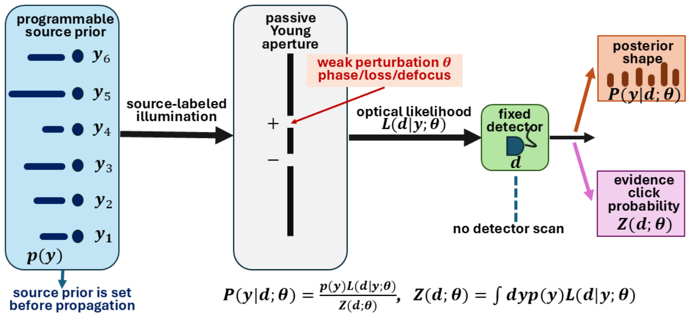
Figure 2.
Source-space response landscape for the balanced double-slit TRY model. (a) Fixed-detector likelihood . (b) Detected posterior for a uniform source prior over the displayed phase interval. (c) Phase score , clipped for display near the source-space nulls. (d) Information density . The figure shows that near-null response enhancement must be judged together with posterior weight: the local score can grow strongly near a null, while the experimentally useful information density remains finite.
Figure 2.
Source-space response landscape for the balanced double-slit TRY model. (a) Fixed-detector likelihood . (b) Detected posterior for a uniform source prior over the displayed phase interval. (c) Phase score , clipped for display near the source-space nulls. (d) Information density . The figure shows that near-null response enhancement must be judged together with posterior weight: the local score can grow strongly near a null, while the experimentally useful information density remains finite.
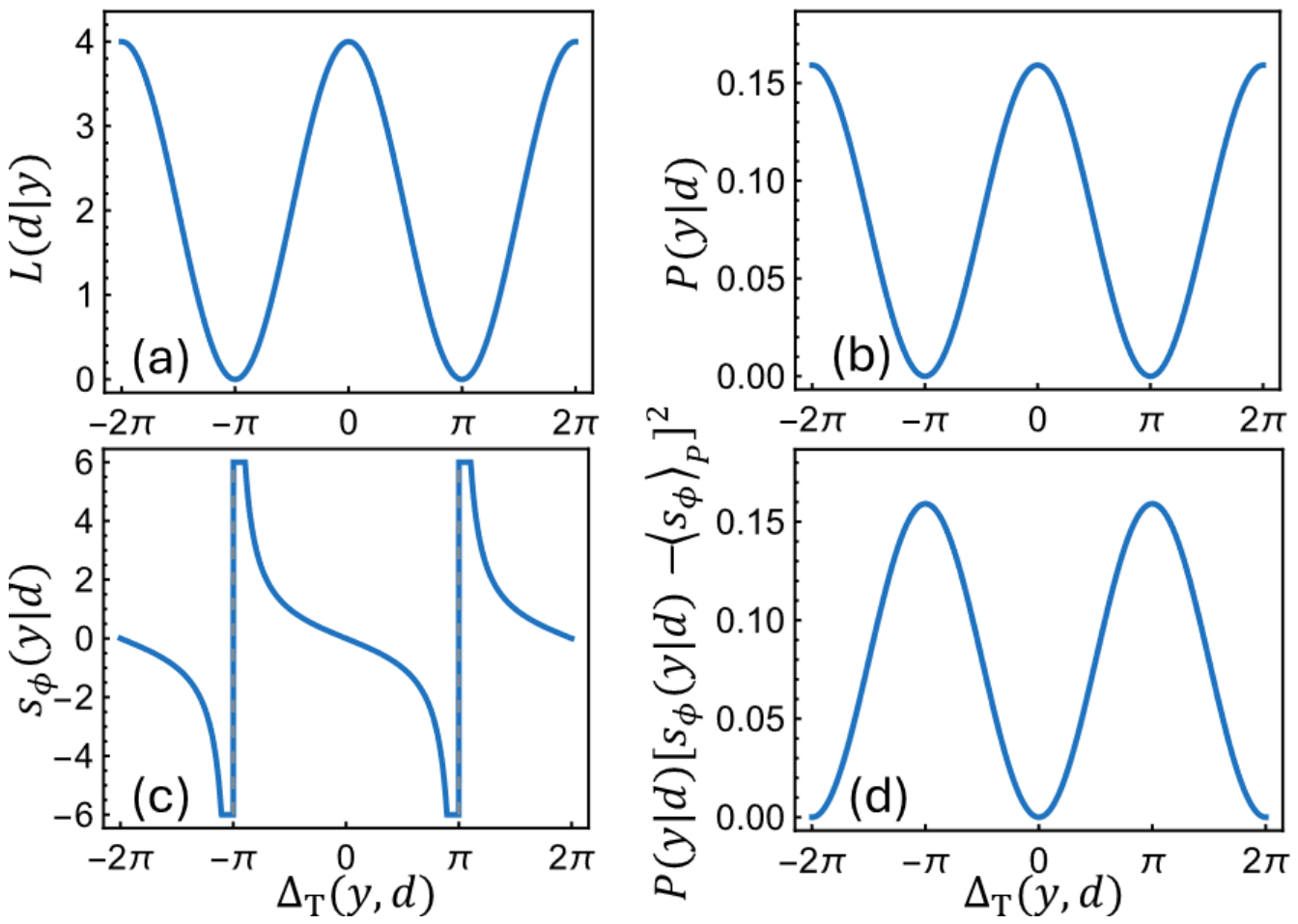
Figure 3.
Two-label source-prior engineering in TRY. (a) A preliminary fixed-detector source scan gives the likelihood landscape , from which two source labels and are selected. (b) The same labels are chosen to have strong phase-score contrast , where . (c) Because the two labels generally have different likelihoods, the programmed prior weights are chosen according to , producing balanced detected posterior weights . (d) A weak one-slit phase perturbation is then read out as the differential label imbalance . The dashed line shows the linear response .
Figure 3.
Two-label source-prior engineering in TRY. (a) A preliminary fixed-detector source scan gives the likelihood landscape , from which two source labels and are selected. (b) The same labels are chosen to have strong phase-score contrast , where . (c) Because the two labels generally have different likelihoods, the programmed prior weights are chosen according to , producing balanced detected posterior weights . (d) A weak one-slit phase perturbation is then read out as the differential label imbalance . The dashed line shows the linear response .
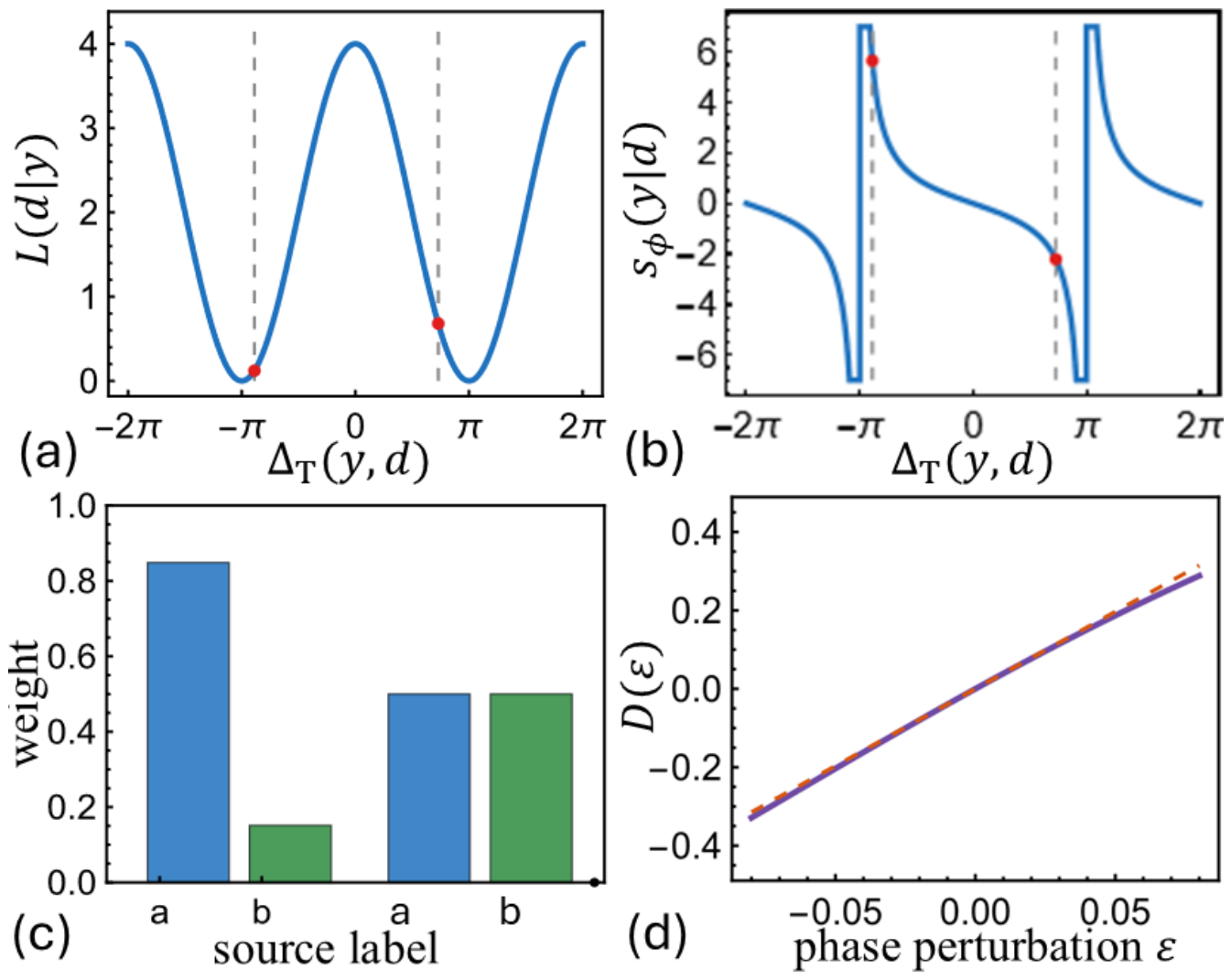
Figure 4.
Multiparameter source-prior design in TRY. (a) Target phase score for a slightly imbalanced two-path model. (b) Nuisance loss score over the same source-label coordinate. (c) Score-vector trajectory , showing how selected labels populate the two-dimensional score space. (d) Covariance metrics for the selected three-label code: target information , cross covariance , and nuisance-eliminated information . The red points mark the selected source labels. The figure shows how a source code can retain target sensitivity while suppressing target–nuisance covariance.
Figure 4.
Multiparameter source-prior design in TRY. (a) Target phase score for a slightly imbalanced two-path model. (b) Nuisance loss score over the same source-label coordinate. (c) Score-vector trajectory , showing how selected labels populate the two-dimensional score space. (d) Covariance metrics for the selected three-label code: target information , cross covariance , and nuisance-eliminated information . The red points mark the selected source labels. The figure shows how a source code can retain target sensitivity while suppressing target–nuisance covariance.
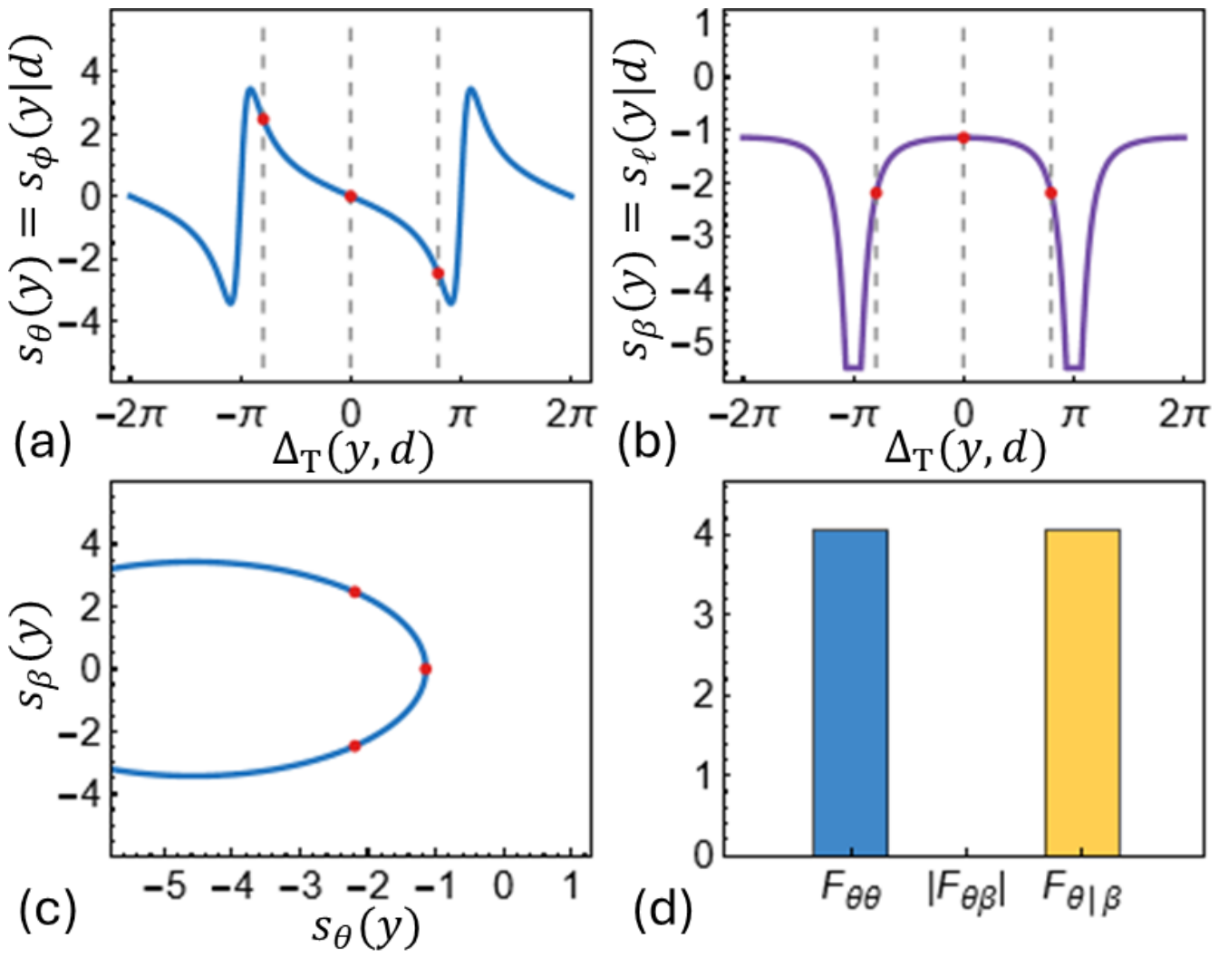
Figure 5.
Double-slit TRY response to one-slit perturbations. (a) Fixed-detector likelihood for a two-path model with path-amplitude ratio . (b) Phase score , obtained from a weak one-slit phase perturbation and proportional to . (c) Loss score , obtained from a weak one-slit amplitude-loss perturbation and proportional to . (d) Complex path-weight trajectory reconstructed from . The dashed vertical lines in panels (a)–(c) mark the balanced-model source-space nulls. For , the loss score is constant; for , path imbalance makes the real part of the path response source-label dependent.
Figure 5.
Double-slit TRY response to one-slit perturbations. (a) Fixed-detector likelihood for a two-path model with path-amplitude ratio . (b) Phase score , obtained from a weak one-slit phase perturbation and proportional to . (c) Loss score , obtained from a weak one-slit amplitude-loss perturbation and proportional to . (d) Complex path-weight trajectory reconstructed from . The dashed vertical lines in panels (a)–(c) mark the balanced-model source-space nulls. For , the loss score is constant; for , path imbalance makes the real part of the path response source-label dependent.
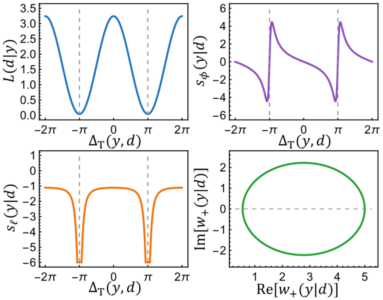
Figure 6.
Experimental workflow for source-prior engineering in TRY. A broad fixed-detector source scan with a uniform or broad prior records baseline and perturbed source-label counts, from which the likelihood and score are estimated. These response maps are then used to design a source code, for example by choosing two labels with large score separation and setting dwell times according to to balance the detected posterior. The optimized sensing scan is a second physical acquisition at the same fixed detector and yields the counts used to compute the differential imbalance D, centered susceptibility , detected-event Fisher information , evidence , and throughput-weighted information . A conventional Young control uses the same aperture and perturbation but replaces source-side programming with detector-plane sampling, enabling a direct comparison of posterior-shape response, evidence, throughput, and hardware-calibration trade-offs.
Figure 6.
Experimental workflow for source-prior engineering in TRY. A broad fixed-detector source scan with a uniform or broad prior records baseline and perturbed source-label counts, from which the likelihood and score are estimated. These response maps are then used to design a source code, for example by choosing two labels with large score separation and setting dwell times according to to balance the detected posterior. The optimized sensing scan is a second physical acquisition at the same fixed detector and yields the counts used to compute the differential imbalance D, centered susceptibility , detected-event Fisher information , evidence , and throughput-weighted information . A conventional Young control uses the same aperture and perturbation but replaces source-side programming with detector-plane sampling, enabling a direct comparison of posterior-shape response, evidence, throughput, and hardware-calibration trade-offs.
Disclaimer/Publisher’s Note: The statements, opinions and data contained in all publications are solely those of the individual author(s) and contributor(s) and not of MDPI and/or the editor(s). MDPI and/or the editor(s) disclaim responsibility for any injury to people or property resulting from any ideas, methods, instructions or products referred to in the content. |
© 2026 by the authors. Licensee MDPI, Basel, Switzerland. This article is an open access article distributed under the terms and conditions of the Creative Commons Attribution (CC BY) license (http://creativecommons.org/licenses/by/4.0/).
Copyright: This open access article is published under a Creative Commons CC BY 4.0 license, which permit the free download, distribution, and reuse, provided that the author and preprint are cited in any reuse.


