

Submitted:
01 July 2026
Posted:
03 July 2026
You are already at the latest version
Abstract
This article presents the authors’ proposed theory on the formation of cavitation voids in the false vacuum during the inflationary phase of the Big Bang. It examines the structure of, and the physical processes occurring in, the transition region at the boundary between the false and physical vacuums. It has been demonstrated that, during the formation of physical vacuum voids (regions in which the Λ-term, a constant in the equations of general relativity, goes to zero), conditions arise in the transition region between the false vacuum and the physical vacuum that allow for the formation of a narrow layer of matter. This layer may be the precursor to the bridges observed in the large-scale lattice structure of the universe. The mechanism of bubble expansion during the inflationary phase of the universe is examined. It has been demonstrated that the inflationary phase of expansion passes into the standard Big Bang model due to the conversion of the false vacuum into matter at the boundaries of the bubbles. This model does not require the universe to undergo an extremely rapid expansion to explain the quasi-homogeneous and isotropic distribution of matter and the cosmic microwave background. Furthermore, it can account for the formation of the large-scale lattice structure of the universe. The estimated radii of cosmic voids are consistent with observational data.
Keywords:
big band
; inflation stage
; cavitation
; cosmic voids
1. Introduction
One of the main problems with the Lemaître–Gamow Big Bang theory is the striking homogeneity of matter distribution in our universe, as well as the isotropy of the cosmic microwave background radiation (CMB) [1,2], which was discovered in 1964 by Penzias and Wilson [3] and had been previously predicted by Gamow [4]. Small fluctuations in the density of matter during the early stages of the expanding universe should have resulted in obvious inhomogeneities in matter distribution today. Furthermore, there is no clear, consistent explanation for the observed clustered structure of visible matter in the universe, nor for its homogeneity on scales exceeding 100 megaparsecs [1,2]. While the inflationary model of the early expansion of the universe, as proposed by Guth [5] and further developed by Linde [6,7,8,9,10], Vilenkin [11,12,13,14] and others [15,16,17,18,19,20,21,22,23,24,25,26,27,28], can explain the observed isotropy and homogeneity of the cosmic microwave background (CMB), the large-scale lattice structure of matter distribution in the universe still raises many questions (see, for example, [29]).
In [30], we proposed a cavitation model of the inflationary stage of the Big Bang. In this model, the cosmological constant Λ-term in the equations of general relativity behaves like negative pressure in a fluid. If this constant exceeds a certain critical value Λ_cr, then discontinuities, or bubbles, arise in spacetime where the Λ-term is zero. The appearance of these bubbles naturally reduces the average value of the cosmological constant, thereby slowing down the expansion rate of the universe.
Clearly, the average value of the Λ-term in any region of spacetime cannot exceed the threshold value. Exceeding the threshold leads to the formation of new voids (bubbles), while falling below it results in a decrease in bubble density due to spreading. Consequently, the absolute value of Λ increases up to the threshold value. Consequently, the absolute value of the Λ-term increases up to the threshold value. [30] also shows that, if they do not grow over time, the emergence of voids cannot halt inflation, but can only slow it down. However, if we assume that the radius of the bubbles increases for some reason, they will gradually displace the false vacuum over time, resulting in a smooth transition from the inflationary phase to the classical Lemaitre–Gamow expansion. Within the framework of the cavitation model of the early stages of the universe’s expansion [30], the uniform distribution of matter in the universe is naturally explained and does not require super-rapid expansion, as proposed in the theories of Guth, Linde, Starobinsky, Vilenkin and others .
This paper demonstrates that conditions can arise for the formation of narrow, matter-filled layers during the development of physical vacuum bubbles in the transition region between the false vacuum and the true (physical) vacuum. These layers may serve as precursors to the filaments and nodes observed in the large-scale cellular structure of the Universe (the cosmic web).
We examine the expansion of voids during the inflationary phase of the Universe and show that the conversion of false vacuum energy into matter at bubble boundaries drives the transition from the inflationary stage to the standard Big Bang evolution. We propose that thin, gravitating matter layers formed at the boundaries of false vacuum decay may act as sites of dark matter concentration and may themselves be considered a form of dark matter. In other words, dark matter and dark energy may be connected to each other.
Section II presents a detailed analysis of the model describing void formation during the inflationary stage. It highlights both similarities to and differences from void formation in liquids and solids under tensile stress.
Section III investigates an individual bubble within the false vacuum region, demonstrating that a potential well forms at its boundary, acting as a collector for particles generated there.
Section IV analyzes the formation of a thin layer of gravitating matter at the interface between the true (physical) and false vacuum states.
Section V employs an analogy with a combustion wave to develop a simple empirical model for the conversion of false vacuum energy into dark matter. We derive the expansion velocity of a bubble nucleated in the false vacuum and show that, within a finite time, bubbles approach one another closely enough for the Universe to transition from a continuous medium into a cosmic web, with most gravitating mass concentrated in filaments. The estimated radii of cosmic voids are consistent with observational data.
Section VI discusses the main results and future directions of the cavitation-based approach presented here, along with its implications for Big Bang–type cosmological models.
Section VII summarizes the conclusions of the study.
2. Formation of Physical Vacuum Bubbles Within the False Vacuum
The equations of general relativity in their general form are given by [31]:
In equation (1), is the speed of light, is Einstein’s cosmological constant, is Newton’s gravitational constant, and is the energy–momentum tensor of matter; expressions for the Ricci tensor and the scalar curvature in terms of the metric tensor can be found in [31], and is the unit 4-tensor.
The left-hand side of equation (1) describes the geometry of spacetime, while the right-hand side represents the distribution of energy and momentum within it. Comparing equation (1) with Maxwell’s equations, the left-hand side is analogous to the distribution of the electromagnetic field, and the right-hand side corresponds to the distribution of electric charges and currents in space.
In problems of general relativity, the energy–momentum tensor is usually specified (analogous to the distribution of charges and currents in Maxwell’s equations), and then equation (1) is solved to determine the curvature of spacetime and the distribution of the energy–momentum tensor in the coordinate system .
The interval in a synchronous coordinate system, for a homogeneous and isotropic distribution of matter in space, takes the form of the Friedmann–Lemaître–Robertson–Walker (FLRW) metric [32,33]:
The solution of equation (1) for the interval (2) has the form [32,33]:
Here, the dots above denote derivatives with respect to time, in (4) can take the values . Below, we consider equations (3) and (4) in the de Sitter model with . For empty space, where , the solution of equations (3)-(4) is given by:
Following Guth’s work, we will refer to the exponential expansion of the Universe (6) as inflation.
The presence of the term in Einstein’s equation (1), by analogy with liquids and solids under tensile forces, is often interpreted as negative pressure; however, this interpretation is not entirely correct. Therefore, before discussing the formation of cavitation voids of the physical vacuum within the false vacuum, we first consider how cracks form in elastic solids. Let us write down Hooke’s law for a medium possessing elasticity. In the case of uniform compression or expansion of a sphere of radius , we have [34]:
Here, is the displacement of points along the radius of the sphere, is the pressure inside the body associated with applied external forces, and is the bulk modulus. From equation (7), it follows that the relative change in the radius of the sphere is given by:
That is, it is proportional to the internal stress . The difference between equations (8) and (5) is as follows: in (8), an increase in leads to the relative elongation of the object, whereas in (5), an increase in results in an increase in the relative expansion rate of the Universe.
We know that any solid body in a field of tensile forces has a limit of strength: if the stress exceeds a certain value, cracks or cavities form in the material. This raises the question: is there a strength limit of spacetime under tensile forces?
Let us adopt the hypothesis that the strength limit of spacetime, unlike that of elastic bodies, is determined not by the relative change in distance between points, , but by the relative rate at which they move apart, .
If in a certain region of spacetime the relative rate of change of distances, , exceeds a critical value, , then cracks must form in this region – areas where the tensile stress and, accordingly, . In other words, if the relative expansion rate of the Universe in any region does not exceed a certain threshold:
no cracks form, and the Universe expands exponentially.
It should be noted that is not limited by the speed of light, since the expansion of the Universe is not associated with the transfer of mass or energy.
2.1. The Cavitation Model of the Inflationary Phase of the Universe’s Expansion
We consider the regime in which the dynamics of spacetime are governed solely by the cosmological constant term in the Einstein field equations. The issue of a possible conversion of dark energy into gravitating mass will be addressed in Section III. For , the Universe expands according to Eq. (6). In contrast, if , our hypothesis implies that regions (voids) with nucleate in spacetime and continue to form until the volume-averaged cosmological constant reaches .
Since we assume that and its critical value are uniform throughout space, one would expect that –just as in the development of cavitation in an ordinary liquid [35,36] – the voids produced by false vacuum decay would be distributed approximately uniformly throughout the entire volume of the Universe. Indeed, if in some region of the Universe , the number of bubbles will begin to grow, and this process will continue until decreases to . If, within a given region of the Universe, falls below , the mechanism responsible for maintaining its constancy - analogous to a field of negative pressure (tension) in a continuous medium (liquids or solids) - acts to increase , thereby leading to the formation of new ruptures. Accordingly, a new cosmological constant equal to should be established in the Universe. We relate the value of to the relative volume of the physical vacuum within the false vacuum. Let the scale in Eq. (1) be much larger than the size of a vacuum bubble . Then, the relative volume occupied by bubbles of the true vacuum (where ) within the false vacuum is given by:
Where is the number of bubbles per unit volume, is the initial radius of the cavitation bubble. The relative volume occupied by the false vacuum is equal to , therefore and according to (9)
Equation (11) implies that if the fractional volume occupied by bubbles of the true vacuum remains constant , then the inflationary expansion cannot be terminated,
It is important to distinguish between cavitation in spacetime and in a fluid. As shown in [35,36], the generation of cavitation bubbles, both in ordinary and cryogenic liquids, reduces the negative pressure to a level at which further bubble nucleation ceases. At the same time, the radius of bubbles already formed in the liquid continues to increase, since the magnitude of the negative pressure remains greater than the Laplace pressure. This leads to a further decrease of the negative pressure in the cavitation region [35,36]. In spacetime, however, there is no natural mechanism for bubble growth, since spacetime itself undergoes expansion. In our view, the only mechanism capable of terminating inflation is the conversion of the false vacuum energy into gravitating matter (both dark and baryonic) at the boundaries of the bubbles. This process is analogous to conventional cavitation in a fluid, where the excess energy associated with negative pressure is expended on bubble formation, their expansion, and the surface tension energy. In our case, the role of surface tension is played by the gravitating mass concentrated on the surfaces of the discontinuities (see Section III).
2.2. Simplified Approach to Inflationary Stage Saturation in the Expanding Universe
Since the distribution of cavitation bubbles in space is homogeneous and time-independent, let us assume that the relative volume of bubbles in a given region of space grows at a rate proportional to the relative volume occupied by the false vacuum. (A more accurate model of nucleation will be discussed in Section III.)
Here, is a dimensionless parameter characterizing the expansion rate of a physical vacuum bubble. Accordingly:
Substituting (14) into (13), we obtain:
and, correspondingly
This implies that both the duration of the inflationary phase and the relative expansion of the Universe are limited, specifically: and .
Figure 1 shows the evolution of and for various values of .
Figure 2 shows the distribution of true vacuum voids that appeared at different times during the process of inflationary expansion.
In Section IV, it will be shown that all gravitational mass (both dark matter and visible matter) accumulates at the boundaries of the bubbles.
3. A Single Void of Physical Vacuum Within the False Vacuum
Consider the space-time metric in the reference frame associated with the center of a spherically symmetric true vacuum bubble, surrounded by a false vacuum (Figure 3), for times much smaller than the characteristic expansion time of the universe, , where is the typical expansion time in standard inflationary models [5,6,7,8,9,10,11,12,13,14].
As in [30,37,38], the transition region at the boundary between the false vacuum and the true (physical) vacuum will be described using the De Sitter metric. Following [31], in the case of spherical symmetry, in terms of the coordinates can be written as:
In this case, Einstein’s equations are rewritten in the form given in [30,31]:
In equations (18)-(21), the dots above and denote derivatives with respect to time, while the primes denote derivatives with respect to the coordinate .
We seek a stationary solution of (18)-(21) in the regions of the false vacuum () and the physical vacuum (), where is the radius of the formed bubble of physical vacuum (Figure 3). We assume that and far from the boundary in the false vacuum region (), and in the physical vacuum region.
It can be shown that in stationary case, it is impossible to match the solutions at the boundary between the physical and false vacuums (Figure 1) without accounting for in (18)–(20). Indeed, in the stationary case, equations (18)-(20) take the form
Subtracting (23) from (22), we obtain, . Substituting in (23) and (24) we have
Multiplying (25) by and differentiating along the radius, we get:
When obtaining (27), we considered that in the transition region . Comparing the left-hand sides of (27) and (26) (the right-hand sides are the same) we get that . In other words, it is impossible to describe the region of transition of a real vacuum to a false one by one function . The formation of a bubble of physical vacuum always occurs with the formation of matter, characterized by the energy-momentum tensor .
As in [30,37,38,39,40], we put . In this case, the system of equations (18) - (21) is reduced to the equations:
Recall that , and all other components of are equal to zero. We rewrite (28) and (29) as follows:
From (30) it follows:
In the absence of the Λ term, Eqs. (18)-(21) reduce to the equations governing a spherically symmetric field [34]. It then follows that for all values of .
To match Eq. (30) in the false vacuum region () with the solution in the physical vacuum region (), we assume that the size of the transition region from the false vacuum to the physical vacuum is much smaller than . In this case, one can write:
where – the value of the cosmological constant out of the bubble of the physical vacuum, is an independent parameter of the problem. We assume that in the false vacuum region, far from the transition boundary, , so that the curvature is determined solely by , . We determine the free parameter in Eq. (34) from the condition:
Substituting Eqs. (30) and (31) into (35), we obtain:
Figure 4 shows the dependence of on in terms of the dimensionless variables
It is evident that the asymptotic behavior of with respect to and is consistent with Eq. (36).
Substituting the dimensionless forms of and from Eqs. (33) and (34) into the Einstein equations (31) and (32) yields:
Equation (38) gives the dimensionless metric function in terms of the energy density and the interpolated cosmological constant, while Eq. (31) determines the transverse pressure component in terms of the radial energy density and the derivative of the cosmological constant. In these expressions, the energy density peaks at the bubble wall and vanishes far from it, so that the spacetime curvature is dominated by in the false vacuum region.
Figure 5 shows the dependence of , , and on , as well as the behavior of .
Consider the forces acting on particles in the regions of the false and true vacuum. Assuming that the gravitational field at the discontinuity is time-independent, the force acting on a particle of mass in the centrally symmetric case, according to [31, Problem 1, formula (3)] for interval (1), is given by:
where is the relativistic mass of the particle ( is the rest mass, is the velocity). In Eq. (40) we have considered that the metric component (see Eq. (1)).
The potential energy of a particle corresponding to the force in dimensional variables is given by:
For , the contribution of in Eq. (40) can be neglected. Using the asymptotic expression for the metric component at , , we obtain the asymptotic values of the force and potential energy:
Figure 6 shows the dependence of the reduced quantities and on .
The role of dark matter as a potential barrier for particles within a true vacuum bubble is not surprising, since the effective force associated with the false vacuum is always directed toward regions where it is absent. This conclusion remains valid under the assumption that either the characteristic size of the true vacuum bubble is sufficiently small or the value of in its vicinity is sufficiently low, so that the effects of cosmic expansion can be neglected.
Figure 7 shows the dependence of on for and . According to [31], the points where changes sign indicate the presence of an event horizon. It should be noted that, unlike ordinary black holes, in this case there are always two horizons, similar to the case of a black hole with a dark energy core [38].
It is well known (see, e.g., [41,42,43]) that tidal forces arise at the event horizon. These forces are so strong that they first break molecular bonds, then ionize atoms, and finally disrupt nuclear binding. As a result, at the boundary of the event horizon, matter is reduced to a soup of neutrons, protons, and electrons.
In [38], it is shown that, in a distant reference frame, electrons, protons, and neutrons cross the event horizon over a time scale, where is the radius of the event horizon, is the Compton wavelength of the particle, is its mass, and is the reduced Planck constant. This effect is explained by the manifestation of the wave properties of particles in the vicinity of the event horizon.
In this work, we limit ourselves to noting the possible formation of an event horizon in the transition region between the false and true vacuum. Figure 7 shows the dependence of the critical value on .
4. Formation of a Thin Layer of Matter at the Boundary Between the Physical and False Vacuum
Let us consider the creation of particle–antiparticle pairs within a bubble of the physical vacuum, as illustrated in Figure 3. The transition layer separating the false vacuum from the true (physical) vacuum consists of a mixture of dark energy, characterized by the cosmological constant , and matter, characterized by the energy–momentum tensor . In this region, gravitational forces attain their maximum strength (see Figure 6A). Since gravitational forces acting on particles and antiparticles are independent of the sign of their electric charge, their separation can occur only in the presence of a gradient in the gravitational field, i.e., tidal forces.
The work performed by tidal forces to separate a particle–antiparticle pair over a distance of the order of their Compton wavelength, , where is the reduced Planck constant and is the particle rest mass, is given by
Folowing [44], the probability of particle–antiparticle pair creation, up to numerical factors of order unity, can be estimated as
This expression shows that pair production is exponentially suppressed when the work performed by the tidal forces over a Compton wavelength is much smaller than the particle rest energy .
Introducing the critical tidal-force gradient
Eq. (44) can be rewritten in the form
Thus, efficient particle–antiparticle pair production occurs when the tidal-force gradient approaches or exceeds the critical value . For | |≪ , the production rate is exponentially suppressed.
Equation (46) has the same functional form as the Schwinger formula for the probability of electron–positron pair production in a constant electric field. In the present case, however, the role of the electric field strength is played by the gradient of the gravitational force (the tidal-force gradient).
Introducing dimensionless variables, the critical condition for efficient particle–antiparticle pair production can be written as
where is the dimensionless critical tidal-force gradient.
Figure 8 shows the distribution of the tidal-force gradient as a function of . As expected, the tidal forces are concentrated at the boundary of the physical-vacuum bubble.
Substituting Compton wavelength of an electron in Eq. (47), we obtain
For neutrinos, whose mass is currently estimated to be approximately times smaller than the electron mass, the corresponding critical value is
Thus, the threshold tidal-force gradient required for particle–antiparticle pair production is many orders of magnitude lower for neutrinos than for electrons. Consequently, neutrino–antineutrino pair production is expected to become significant under considerably weaker tidal gravitational fields.
Since a rigorous theory of particle–antiparticle pair production in a gravitational field lies beyond the scope of the present work, we restrict our analysis to the estimate given by Eq. (45) and consider only the dynamics of massive particles generated within the physical-vacuum region.
Without loss of generality, we assume that throughout the particle-production region, i.e., that no event horizons are present there, as illustrated in Figure 7. Under these conditions, the following scenarios are possible, as shown in Figure 9. Both particles may escape from the transition layer if their energies satisfy the condition . Alternatively, both particles may be trapped in the potential well if their energies satisfy . Finally, one particle may remain trapped while the other escapes from the transition layer.
Consider the fate of an emitted particle. The potential wells at the boundaries of an expanding physical vacuum bubble are shown schematically in Figure 10. If the expansion velocity of the bubble boundary is smaller than the particle’s initial velocity , then when the particle reaches the opposite wall, its velocity relative to that wall is reduced compared to its initial value. Consequently, after an elastic reflection, the particle’s kinetic energy in the laboratory frame decreases.
The particle will continue to bounce between the walls, gradually losing energy, until it is eventually captured in either the left or right potential well shown in Figure 10, for example, through scattering with particles already trapped in the wells.
After each elastic reflection, the particle’s velocity decreases by an amount equal to . Let us estimate the rate of energy loss for a relativistic particle undergoing repeated collisions with the walls of a physical vacuum bubble expanding at a constant velocity.
Without loss of generality, let us consider the simplest case in which the expansion velocity of the physical vacuum bubble is constant and much smaller than the speed of light. In this regime, collisions of particles with the expanding bubble walls (Figure 10) can be treated within the classical approximation. For simplicity, we also assume that the collisions of particles with the walls are elastic.
Suppose that a particle is created in the transition layer at the left boundary with velocity . In the laboratory frame of reference (associated with the center of the bubble), its velocity is , while in the frame associated with the right wall it is (the -axis is directed from left to right). After an elastic collision with the right wall, the particle is reflected toward the left. Its velocity in the frame of reference associated with the left wall is then .
It follows that after each elastic collision with a wall; the magnitude of the particle’s velocity decreases by in the frame of reference of the opposite wall. This deceleration process continues until the particle’s velocity in the laboratory frame becomes smaller than .
The recurrence relations connecting the time between successive collisions with the bubble walls to the particle velocity and the bubble expansion rate after the -th collision can be written as
where is the dimensionless expansion velocity of the bubble, is the dimensionless bubble radius, is the particle velocity after the -th collision, and is the dimensionless time interval between successive collisions of the particle with the bubble walls. Here, is the bubble radius at the moment of particle creation, and is the initial particle velocity in the reference frame in which it is created.
Table 1 presents an example of calculations based on the recurrence relations (50) for the initial particle velocity , the initial radius , and .
In this work, we do not consider the thermalization of trapped particles over time due to collisions between them (i.e., the establishment of a thermal, Maxwellian distribution and the emergence of a temperature), nor the subsequent filling of the potential well with particles from the transition region.
It should be noted that, for fixed values of and , the depth of the potential well (see Figure 6) increases over time, so that the energy distribution of particles in the well evolves as , where is the Boltzmann constant.
It should be noted that the presence of event horizons within the transition layer does not fundamentally alter the particle dynamics described above. As shown in [38], in the laboratory reference frame any particle crosses the event horizon within a finite time
Where is the event-horizon radius and is the particle Compton wavelength. Furthermore, if the particle energy is positive, the particle emerges from the horizon region (i.e., crosses the domain where ; see Figure 7) within a finite time of the same order. Therefore, the existence of event horizons in the transition layer does not qualitatively affect the escape conditions for particles with positive energies.
5. Conversions of False Vacuum Energy and the Expansion of the Universe
In Part II, we showed that the formation of voids within the false-vacuum region can only slow down the inflationary expansion of the Universe but cannot stop it, provided that the relative volume occupied by physical-vacuum bubbles, , does not increase with time. If, however, grows with time, the duration of the exponential expansion phase becomes finite. In Part III, we considered an isolated physical-vacuum bubble embedded in a false-vacuum background, assuming that the rupture of the false vacuum occurs on a timescale much shorter than that of the cosmological expansion over the corresponding spatial scale. The stationary solutions of the Einstein equations obtained in that analysis show that a gravitating mass is formed at the bubble boundary (Figure 5B), together with a potential well (Figure 6B). In Part IV, we demonstrated that if the tidal forces at the interface between the false and physical vacuum are sufficiently strong, massive particles are produced in this region and subsequently accumulate near the bubble boundaries.
An increase in the gravitating mass within the transition region enhances the tidal forces, thereby increasing the production rate of both massive and massless particles. This, in turn, further increases the gravitating mass, resulting in a positive feedback loop, as illustrated in Figure 11.
In the inflationary theories of Guth, Linde, and Starobinsky, dark energy (the false vacuum) is associated with the cosmological-constant term in Einstein’s equations of General Relativity. Since the gravitational mass is concentrated exclusively within the narrow boundary region of the physical-vacuum bubble, its growth can occur only through the conversion of energy stored in the false vacuum (dark energy).
The construction of a self-consistent theory describing the conversion of dark energy into gravitational mass (both dark and visible matter) lies beyond the scope of the present work. Therefore, in what follows, we restrict ourselves to the simplest model that allows an estimate of the expansion rate of a physical-vacuum bubble embedded in a false-vacuum background.
Figure 12 schematically illustrates the region in which the false vacuum decays (burns) and is converted into a physical vacuum.
Let the energy stored per unit volume of the false vacuum be , and let the energy of dark matter produced per unit time at the boundary of the false vacuum be . Then the equation describing the propagation of the burning wave in the false vacuum takes a simple form:
where is the velocity of the burning front. Assuming and to be constant, we obtain the following estimate for the expansion velocity of a true-vacuum bubble in а false vacuum:
Equation describing the expansion of a true-vacuum bubble:
Here is a dimensionless variable , The first term in (56) is associated with the expansion of the Universe, while the second term corresponds to the conversion of false-vacuum energy into gravitational mass. Integrating (56) yields:
From (55), the relative volume of the true vacuum changes as:
Here, is the number of bubbles generated per unit volume per unit time. In Eq. (58), it is assumed that a bubble created at time will have at time , a radius , where is the initial bubble radius, is the cosmological scale factor, and is the intrinsic growth rate of the physical-vacuum bubble. Thus, the bubble radius increases both due to the expansion of the Universe and due to the local conversion of false vacuum into physical vacuum.
Let us write the phenomenological equation describing the generation of per unit volume of the false vacuum:
where is a parameter characterizing the threshold at which the generation of discontinuities begins, and is a pre-exponential factor.
Substituting (57) into (56), we obtain:
where is the Heaviside step function:
Equation (58) describes the time evolution of the relative volume occupied by bubbles, . Clearly, equation (58) is valid as long as the gravitational mass does not dominate over the false-vacuum mass; in other words, while .
We now establish a connection between the presence of bubbles and the expansion of the Universe. In the de Sitter model (), Eqs. (3)-(4), governing cosmological expansion in the dimensionless variables (39) and , are written as follows:
In Eqs. (60) and (61), , , and denote the averaged values of the cosmological term and of the energy–momentum tensor components over a volume exceeding the size of a bubble (Figure 2). According to [1], electromagnetic radiation is characterized by , , while dust is described by , . Accordingly, we obtain
Subtracting Eq. (62) from Eq. (35), we obtain
From Eq. (62), it follows that
By equating the right-hand sides of (64) and (65), we obtain:
Similarly to (13), the averaged value of Einstein’s cosmological constant evolves as:
It is evident that for , at which , we must set in equations (62) and (64). Accordingly:
For :
For :
The solutions of equations (70)–(71) for , in the case of electromagnetic radiation, are given by:
and for the dust case:
The values , , as well as and , are determined from the matching conditions between solutions (58), (69), (70), and (72),(73). It should be noted that in the limit , solutions (72) and (73) coincide with the known results [1].
Figure 13 presents the numerical results for .
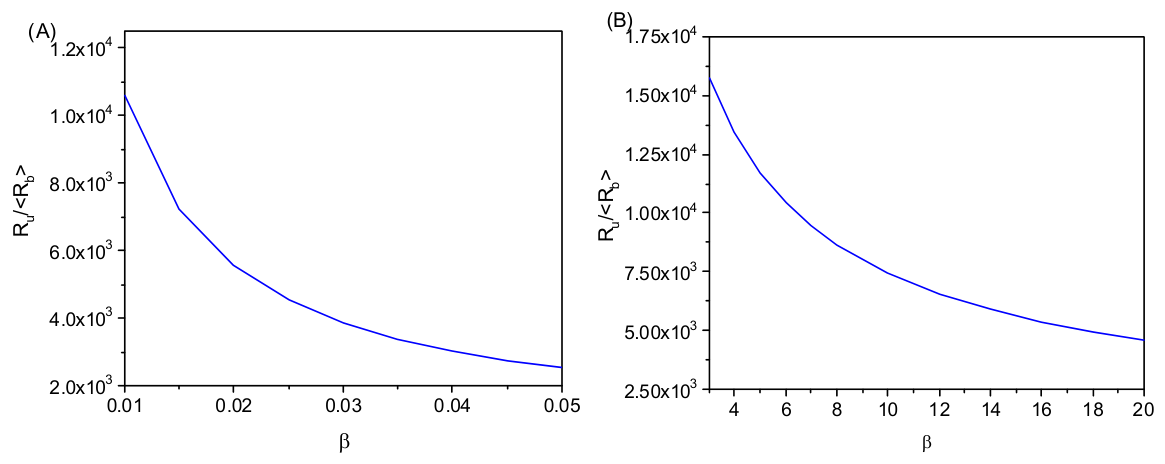
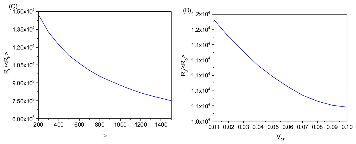
Figure 14 shows the ratio of the Universe radius, , to the mean radius of a physical-vacuum bubble at time , corresponding to the transition to the inertial expansion stage of the Universe (.
6. Discussions
We consider a pre-Friedmann inflationary stage of cosmic expansion that incorporates the cavitation-driven formation of voids within a false vacuum. Since the physical origin of the Big Bang remains unknown, we adopt the working hypothesis that it occurred under conditions in which the cosmological constant, , associated with dark energy, exceeded a critical value, , at which spacetime becomes unstable with respect to the formation of discontinuities. Under such conditions, bubbles of true (physical) vacuum nucleate within the false vacuum, with 0 inside the bubbles. Simultaneously, discontinuities arising at the interfaces between the two phases generate gravitating surface mass, which may be interpreted as dark matter owing to its localized energy–momentum tensor and confinement to the bubble boundaries. Standard-model particles - baryons, leptons, and photons - are assumed to propagate freely within the interiors of these bubbles.
Assuming spatial homogeneity of both and , bubble nucleation through false-vacuum decay leads to an approximately homogeneous distribution of voids throughout the cosmic volume. The dark mass concentrated at the bubble boundaries creates potential wells for particles produced within the true-vacuum regions. However, these particles cannot escape from the bubbles because the surrounding false vacuum, characterized by a nonzero dark-energy density, forms an effectively impenetrable barrier. Consequently, all observable matter is expected to be concentrated within thin boundary layers of thickness δ at the bubble interfaces (Figure 10), where its density is enhanced by a factor of order relative to a hypothetical uniform distribution within the bubble volume.
We further postulate that the interfaces between false and true vacuum support a conversion process (burning), whereby false vacuum is transformed into true vacuum with the simultaneous production of gravitating mass. This process increases the characteristic bubble radius and, correspondingly, the fractional volume occupied by true vacuum, leading to a gradual reduction of the dark-energy density and a deceleration of the inflationary expansion. Because gravitating mass is generated within the true-vacuum regions, the inflationary phase terminates before the false vacuum is completely depleted. Nevertheless, its duration may be sufficiently long to produce an overall expansion of 10–20 orders of magnitude relative to the initial scale. As the false-vacuum fraction, , decreases monotonically with time under the condition , the number of bubbles remains approximately constant, while their characteristic size increases.
The mutual approach and packing of bubbles bounded by thin interfaces naturally give rise to a cellular large-scale structure. It is conceivable that bubble interactions contribute to the formation of supermassive black holes, with dark mass concentrated near their boundaries and dark energy localized toward their interiors. In regions where the dark-energy density decreases, an effective gravitating mass emerges. Within the filamentary structures connecting neighboring voids, where visible matter is concentrated, gravitational (Jeans) instability develops, thereby accelerating the formation of stars and galaxies relative to a uniformly filled Universe.
Although the density of dark energy decreases with time, cosmic expansion does not cease because the gravitating matter within the filaments retains sufficient kinetic energy to sustain it. As the Universe expands and cools, the expansion rate gradually decreases until a transition occurs in which dark energy, potentially stored in compact objects such as black holes [38], once again becomes dynamically dominant. This transition from kinetically driven expansion to dark-energy-driven accelerated expansion may provide a possible explanation for the presently observed cosmic acceleration.
In the present work, we restrict our analysis to a quasi-stationary model of physical-vacuum bubble formation and to a phenomenological description of false-vacuum burning leading to the production of gravitating mass. In addition, bubble–bubble interactions are neglected. We anticipate that future studies employing modern numerical methods for solving the Einstein equations will enable detailed investigations of the dynamics of individual bubbles, both with and without false-vacuum conversion. Such analyses could provide estimates of the epoch at which dark-energy-driven expansion terminates and is replaced by a classical expansion regime governed by the kinetic energy of gravitating matter. It would also be of considerable interest to investigate numerically the dynamics of converging bubbles and to characterize the structures that emerge from their interactions.
7. Conclusions
This paper presents a phenomenological model for the formation of cavitation-induced voids within a false vacuum during the inflationary stage of the Big Bang. We investigate the structure and physical processes occurring in the transition region separating the false vacuum from the physical vacuum. It is shown that the formation of physical-vacuum voids, i.e., regions characterized by a vanishing cosmological term (), naturally leads to conditions favorable for the emergence of a thin layer of gravitating matter at the interface between the two phases. Such layers may represent precursors of the filamentary structures observed in the large-scale cellular distribution of matter in the Universe.
The mechanism governing bubble growth during the inflationary stage is also analyzed. Within the framework of the proposed model, the observed quasi-homogeneous and quasi-isotropic distributions of matter and the cosmic microwave background (CMB) can be reproduced without invoking an extremely rapid expansion of the Universe. In addition, the model provides a possible physical mechanism for the origin of the large-scale cellular structure of the Universe. The estimated radii of cosmic voids are consistent with observational data.
Author Contributions
Conceptualization, M.P. and M.S.; methodology, M.P. and M.S.; formal analysis, M.P. and M.S.; writing—original draft preparation, M.P. and M.S.; writing—review and editing, M.P. and M.S. All authors have read and agreed to the published version of the manuscript.
Funding
This research received no external funding.
Institutional Review Board Statement
Not applicable.
Data Availability Statement
Data are contained within the article.
Conflicts of Interest
The authors declare no conflicts of interest.
References
- Zel’dovich, Ya. B.; Novikov, I. D. Relativistic Astrophysics. In The Structure and Evolution of the Universe; University of Chicago Press: Chicago, 1983; Vol. 2. [Google Scholar]
- Arkhangelskaya, I. B.; Rosenthal, I. L.; Chernin, A. D. Cosmology and Physical Vacuum; (in Russian). KomKniga, Moscow, 2006. [Google Scholar]
- Penzias, A. A.; Wilson, R. W. A measurement of excess antenna temperature at 4080 Mc/s. Astrophys. J. 1965, 142, 419. [Google Scholar]
- Gamow, G. Expanding universe and the origin of elements. Phys. Rev. 1946, 70, 572. [Google Scholar] [CrossRef]
- Guth, A. H. The inflationary universe: A possible solution to the horizon and flatness problems. Phys. Rev. D. 1981, 23, 347. [Google Scholar] [CrossRef]
- Linde, A. D. Print-82-0554 (Cambridge); Nonsingular regenerating inflationary universe. Available online: http://www.stanford.edu/~alinde/1982.pdf.
- Linde, A. D. A new inflationary universe scenario: A possible solution of the horizon, flatness, homogeneity, isotropy and primordial monopole problems. Phys. Lett. B 1982, 108, 389. [Google Scholar] [CrossRef]
- Linde, A. D. Inflation can break symmetry in SUSY. Phys. Lett. B 1983, 131, 330. [Google Scholar] [CrossRef]
- Linde, A. D. Chaotic inflation. Phys. Lett. B 1983, 129, 177. [Google Scholar] [CrossRef]
- Linde, A. D. Eternally existing self-reproducing chaotic inflationary universe. Phys. Lett. B 1986, 175, 395. [Google Scholar] [CrossRef]
- Vilenkin, A. The birth of inflationary universes. Phys. Rev. D. 1983, 27, 2848. [Google Scholar] [CrossRef]
- Vilenkin, A. Predictions from quantum cosmology. Phys. Rev. Lett. 1995, 74, 846. [Google Scholar] [CrossRef] [PubMed]
- Vilenkin, A. Making predictions in eternally inflating universe. Phys. Rev. D. 1995, 52, 3365. [Google Scholar] [CrossRef]
- Vilenkin, A. Many Worlds in One; Hill and Wang, New York, 2007. [Google Scholar]
- Lerche, W.; Lü, D.; Schellekens, A. N. Chiral four-dimensional heterotic strings from self-dual lattices. Nucl. Phys. B 1987, 287, 477. [Google Scholar]
- Tegmark, M.; Aguirre, A.; Rees, M.; Wilczek, F. Dimensionless constants, cosmology and other dark matters. Phys. Rev. D. 2006, 73, 023505. [Google Scholar] [CrossRef]
- Freivogel, B. JCAP 1003; Anthropic explanation of the dark matter abundance. 2010; 021.
- Bousso, R.; Hall, L. Why comparable? A multiverse explanation of the dark matter baryon coincidence. Phys. Rev. D. 2013, 88, 063503. [Google Scholar] [CrossRef]
- Zel’dovich, Ya. B.; Starobinsky, A. A. Quantum creation of a universe in a nontrivial topology. Sov. Astron. Lett. 1984, 10, 135. [Google Scholar]
- Coule, D. H.; Martin, J. Quantum cosmology and open universes. Phys. Rev. D. 2000, 61, 063501. [Google Scholar] [CrossRef]
- Sakharov, A. D. Cosmological transitions with a change in metric signature. Sov. Phys. JETP 1984, 60, 214. [Google Scholar]
- Byrne, P. The Many Worlds of Hugh Everett III; Oxford University Press: Oxford, 2010. [Google Scholar]
- Greene, B. The Hidden Reality; Knopf, New York, 2011. [Google Scholar]
- Tegmark, M. Parallel universes. Sci. Am. 2003, 288, 40. [Google Scholar] [CrossRef] [PubMed]
- Kaku, M. Parallel Worlds; Random House, New York, 2005. [Google Scholar]
- Deutsch, D. The Fabric of Reality; Penguin, London, 1997. [Google Scholar]
- Bousso, R.; Susskind, L. The multiverse interpretation of quantum mechanics. Phys. Rev. D. 2012, 85, 045007. [Google Scholar] [CrossRef]
- Nomura, Y. Physical theories, eternal inflation, and the quantum universe. JHEP 2011 2011, 063. [Google Scholar]
- Thomson, L. A. The Discovery of Cosmic Voids; Cambridge University Press: Cambridge, 2021. [Google Scholar]
- Shneiderm, M. N.; Pekker, M. Cavitation model of the inflationary stage of Big Bang. Phys. Fluids 2021, 33, 017116. [Google Scholar] [CrossRef]
- Landau, L. D.; Lifshitz, E. M. The Classical Theory of Fields, 4th ed.; Elsevier: Oxford, 1975. [Google Scholar]
- Weinberg, S. Gravitation and Cosmology; Wiley: New York, 1972. [Google Scholar]
- Ryden, B. Introduction to Cosmology; Cambridge University Press: Cambridge, 2016. [Google Scholar]
- Landau, L. D.; Lifshitz, E. M. Theory of Elasticity; Pergamon: Oxford, 1970. [Google Scholar]
- Shneider, M. N.; Pekker, M. Liquid Dielectrics in an Inhomogeneous Pulsed Electric Field; IOP Publishing: Bristol, 2019. [Google Scholar]
- Pekker, M.; Shneider, M. N. Sub-barrier cavitation regime in liquid helium. Fluid Dyn. Res. 2025, 57, 065508. [Google Scholar] [CrossRef]
- Pekker, M.; Shneider, M. N. Transitional layer at the edge of a false vacuum in a cavitation model of the Big Bang. arXiv arXiv:2102.01070.
- Pekker, M.; Shneider, M. N. On the possible nature of white holes. Astronomy 2025, 4, 18. [Google Scholar] [CrossRef]
- Dymnikova, I. Cosmological term as a source of mass. arXiv arXiv:gr.
- Dymnikova, I. Universes inside a black hole with the de Sitter interior. Universe 2019, 5, 111. [Google Scholar] [CrossRef]
- Misner, C. W.; Thorne, K. S.; Wheeler, J. A. Gravitation; Freeman: San Francisco, 1973. [Google Scholar]
- Luminet, J. P.; Marck, J. A. Relativistic Roche-Riemann problems around a black hole. Mon. Not. R. Astron. Soc. 1985, 212, 57. [Google Scholar] [CrossRef]
- Kostić, U.; Čadež, A.; Calvani, M.; Gomboc, A. Tidal effects on small bodies by massive black holes. Astron. Astrophys. 2009, 496, 307. [Google Scholar] [CrossRef]
- Shwinger, J. On Gauge Invariance and Vacuum Polarization. Phys. Rev. 1951, 82, 664. [Google Scholar] [CrossRef]
Figure 1.
(A) Dependence of on , according to Eq. (15), and (B) dependence of on , according to Eq. (16). Here, . Line 1 corresponds to , line 2 to , and line 3 to .
Figure 1.
(A) Dependence of on , according to Eq. (15), and (B) dependence of on , according to Eq. (16). Here, . Line 1 corresponds to , line 2 to , and line 3 to .
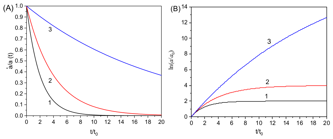
Figure 2.
Distribution of voids at different stages of the inflationary expansion. (A) Initial stage. (B) Intermediate stage — the distance between true vacuum bubbles decreases. (C) End of inflation — matter is concentrated at the bubble boundaries, marking the onset of the Universe’s large-scale cellular structure formation.
Figure 2.
Distribution of voids at different stages of the inflationary expansion. (A) Initial stage. (B) Intermediate stage — the distance between true vacuum bubbles decreases. (C) End of inflation — matter is concentrated at the bubble boundaries, marking the onset of the Universe’s large-scale cellular structure formation.
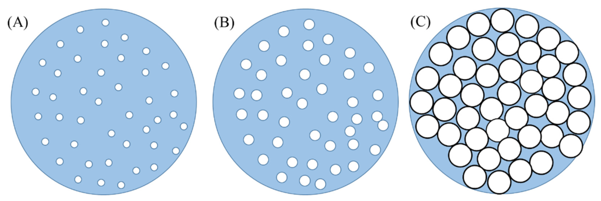
Figure 3.
A spherically symmetric bubble of true vacuum embedded within a surrounding false vacuum.
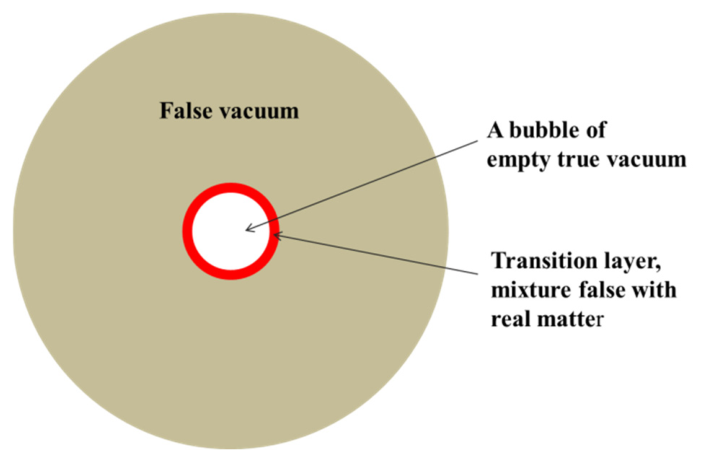
Figure 4.
(A) Dependence of on . Curve 1 corresponds to , curve 2 to , and curve 3 to . (B) Ratio of to its value at as a function of . Curve 1 corresponds to , and curve 2 to .
Figure 4.
(A) Dependence of on . Curve 1 corresponds to , curve 2 to , and curve 3 to . (B) Ratio of to its value at as a function of . Curve 1 corresponds to , and curve 2 to .
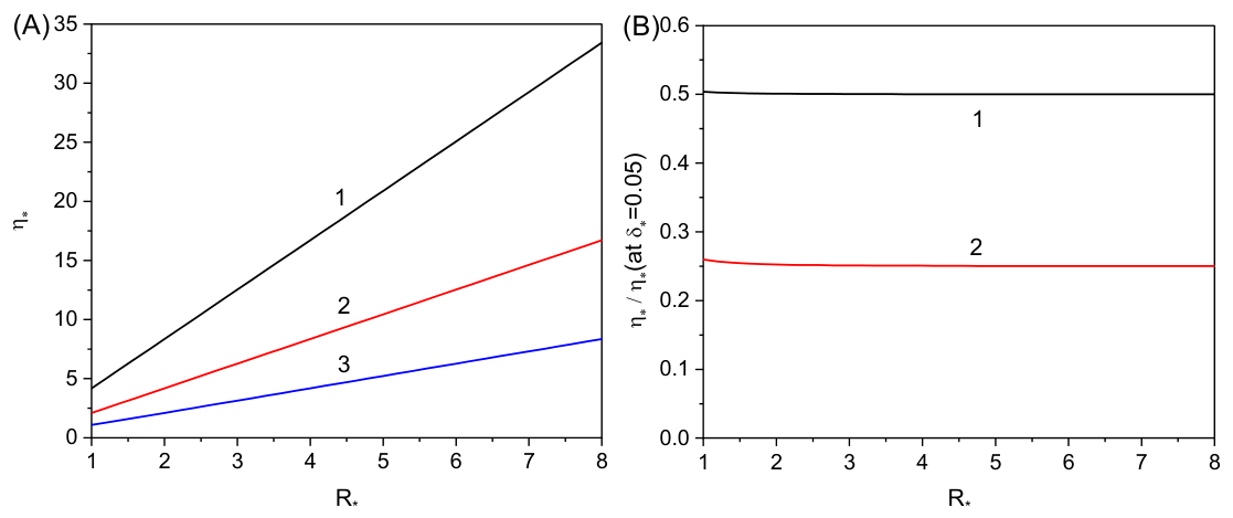
Figure 5.
(A) corresponds to , (B) – to , (C) – to , (D) – to . Line 1 corresponds to , line 2 – to , line 3 – to ;.
Figure 5.
(A) corresponds to , (B) – to , (C) – to , (D) – to . Line 1 corresponds to , line 2 – to , line 3 – to ;.
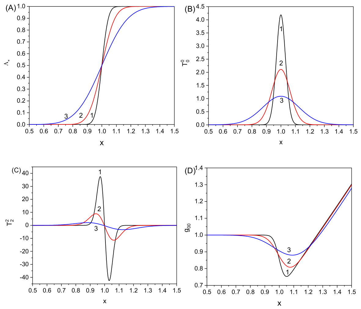
Figure 6.
(A), (B) - Dependence of and on , respectively. Lines 1-3 correspond to , respectively; line 4 corresponds to the asymptotic values from Eq. (40) . The vertical dashed lines in panels (A) and (B) indicate the boundary between real and false vacuum: to the left is the real vacuum, to the right is the false vacuum.
Figure 6.
(A), (B) - Dependence of and on , respectively. Lines 1-3 correspond to , respectively; line 4 corresponds to the asymptotic values from Eq. (40) . The vertical dashed lines in panels (A) and (B) indicate the boundary between real and false vacuum: to the left is the real vacuum, to the right is the false vacuum.
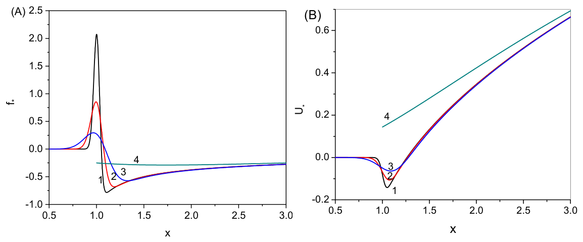
Figure 7.
Dependence of on . (A) corresponds to , (B) – to . Line 1 corresponds to , line 2 – to , line 3 – to . According to [31], the points where change sign indicates the presence of an event horizon.
Figure 7.
Dependence of on . (A) corresponds to , (B) – to . Line 1 corresponds to , line 2 – to , line 3 – to . According to [31], the points where change sign indicates the presence of an event horizon.
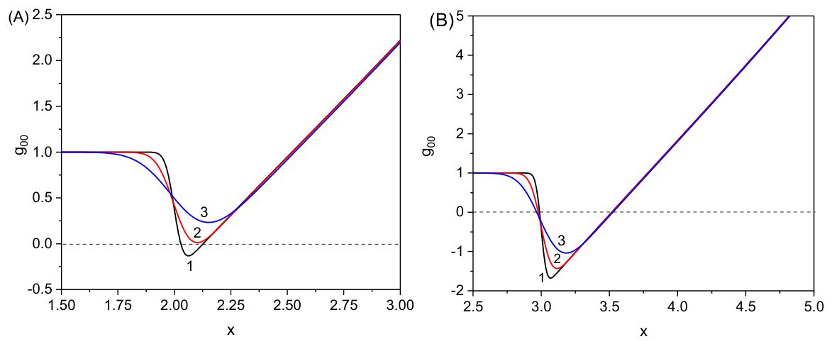
Figure 8.
Dependence of the dimensionless tidal-force gradient on the dimensionless coordinate . Curve 1 corresponds to , curve 2 to , and curve 3 to ; . The dashed lines 1′, 2′, and 3′ indicate the boundaries of the transition region between the false and true vacuum for =0.05, 0.1, and 0.2, respectively.
Figure 8.
Dependence of the dimensionless tidal-force gradient on the dimensionless coordinate . Curve 1 corresponds to , curve 2 to , and curve 3 to ; . The dashed lines 1′, 2′, and 3′ indicate the boundaries of the transition region between the false and true vacuum for =0.05, 0.1, and 0.2, respectively.
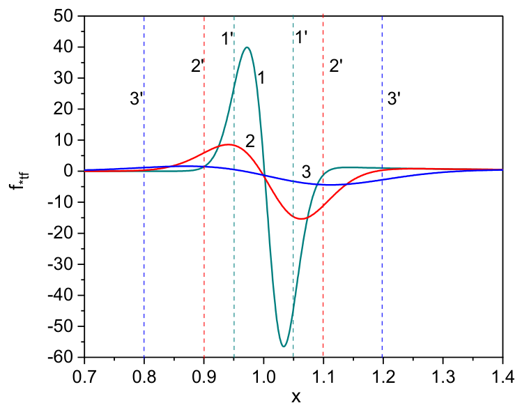
Figure 9.
Potential distribution in the region of the physical vacuum. Particles 1 and 2, created at the interface between the false and true vacua, leave the transition region and move toward the center of the bubble. Particles 5 and 6, produced inside the potential well, are captured and remain within the transition region. For the pair 3 and 4, particle 3 escapes the transition region and moves toward the center of the bubble, whereas particle 4 is trapped in the potential well.
Figure 9.
Potential distribution in the region of the physical vacuum. Particles 1 and 2, created at the interface between the false and true vacua, leave the transition region and move toward the center of the bubble. Particles 5 and 6, produced inside the potential well, are captured and remain within the transition region. For the pair 3 and 4, particle 3 escapes the transition region and moves toward the center of the bubble, whereas particle 4 is trapped in the potential well.
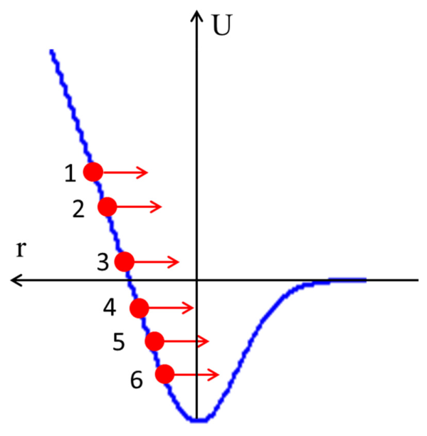
Figure 10.
Transition layers of a physical vacuum bubble within a false vacuum along the -axis, illustrating the motion of a particle inside the bubble as it expands at a constant velocity .
Figure 10.
Transition layers of a physical vacuum bubble within a false vacuum along the -axis, illustrating the motion of a particle inside the bubble as it expands at a constant velocity .
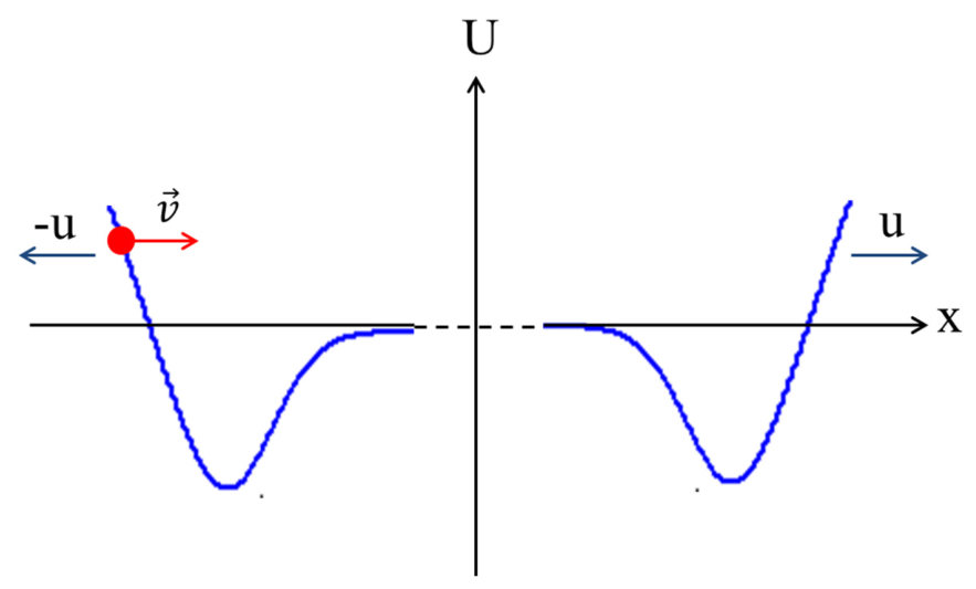
Figure 11.
Tidal forces increase the gravitational mass (both visible and dark matter) within the narrow transition region of a physical-vacuum bubble. At the same time, they reduce the dark energy associated with the -term in Einstein’s equations of General Relativity. Both processes modify the spacetime metric and, consequently, alter the tidal forces themselves, giving rise to a self-consistent feedback mechanism.
Figure 11.
Tidal forces increase the gravitational mass (both visible and dark matter) within the narrow transition region of a physical-vacuum bubble. At the same time, they reduce the dark energy associated with the -term in Einstein’s equations of General Relativity. Both processes modify the spacetime metric and, consequently, alter the tidal forces themselves, giving rise to a self-consistent feedback mechanism.

Figure 12.
Schematic illustration of the boundary of a formed void. Inside the void, the false vacuum is absent (), whereas in the surrounding region , and the false and physical vacua coexist. The region denotes the particle-production zone, and is the radius of the physical-vacuum bubble. Curve 1 corresponds to dark energy (the false vacuum), while curve 2 represents gravitating matter, including both dark and visible matter.
Figure 12.
Schematic illustration of the boundary of a formed void. Inside the void, the false vacuum is absent (), whereas in the surrounding region , and the false and physical vacua coexist. The region denotes the particle-production zone, and is the radius of the physical-vacuum bubble. Curve 1 corresponds to dark energy (the false vacuum), while curve 2 represents gravitating matter, including both dark and visible matter.
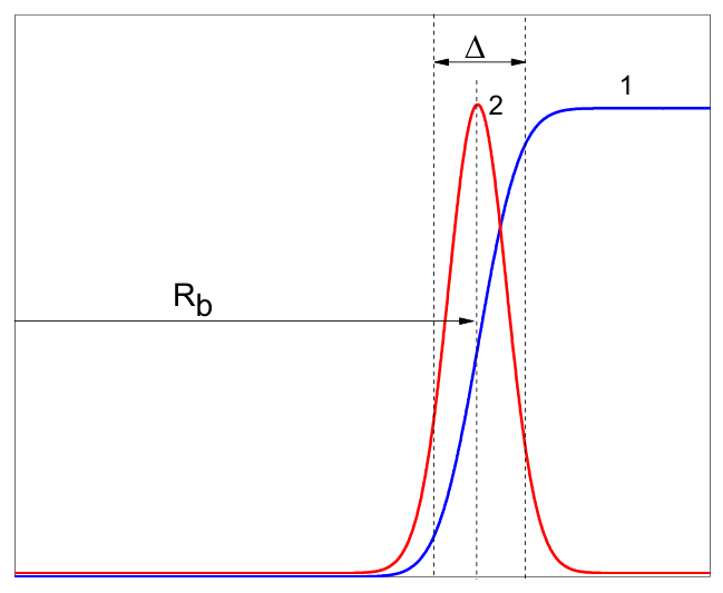
Figure 13.
(A), (B), (E), and (F) Evolution of the Universe size, the Hubble parameter, and the dimensionless energy density as functions of time. (D) Evolution of the dimensionless dark-energy density as a function of time. Lines 1 and 2 correspond to the dust and electromagnetic-radiation cases, respectively. (C) Distribution density of physical-vacuum bubbles as a function of bubble radius. Parameters: , , , , , and .
Figure 13.
(A), (B), (E), and (F) Evolution of the Universe size, the Hubble parameter, and the dimensionless energy density as functions of time. (D) Evolution of the dimensionless dark-energy density as a function of time. Lines 1 and 2 correspond to the dust and electromagnetic-radiation cases, respectively. (C) Distribution density of physical-vacuum bubbles as a function of bubble radius. Parameters: , , , , , and .
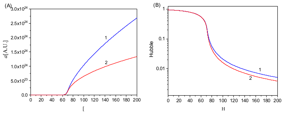
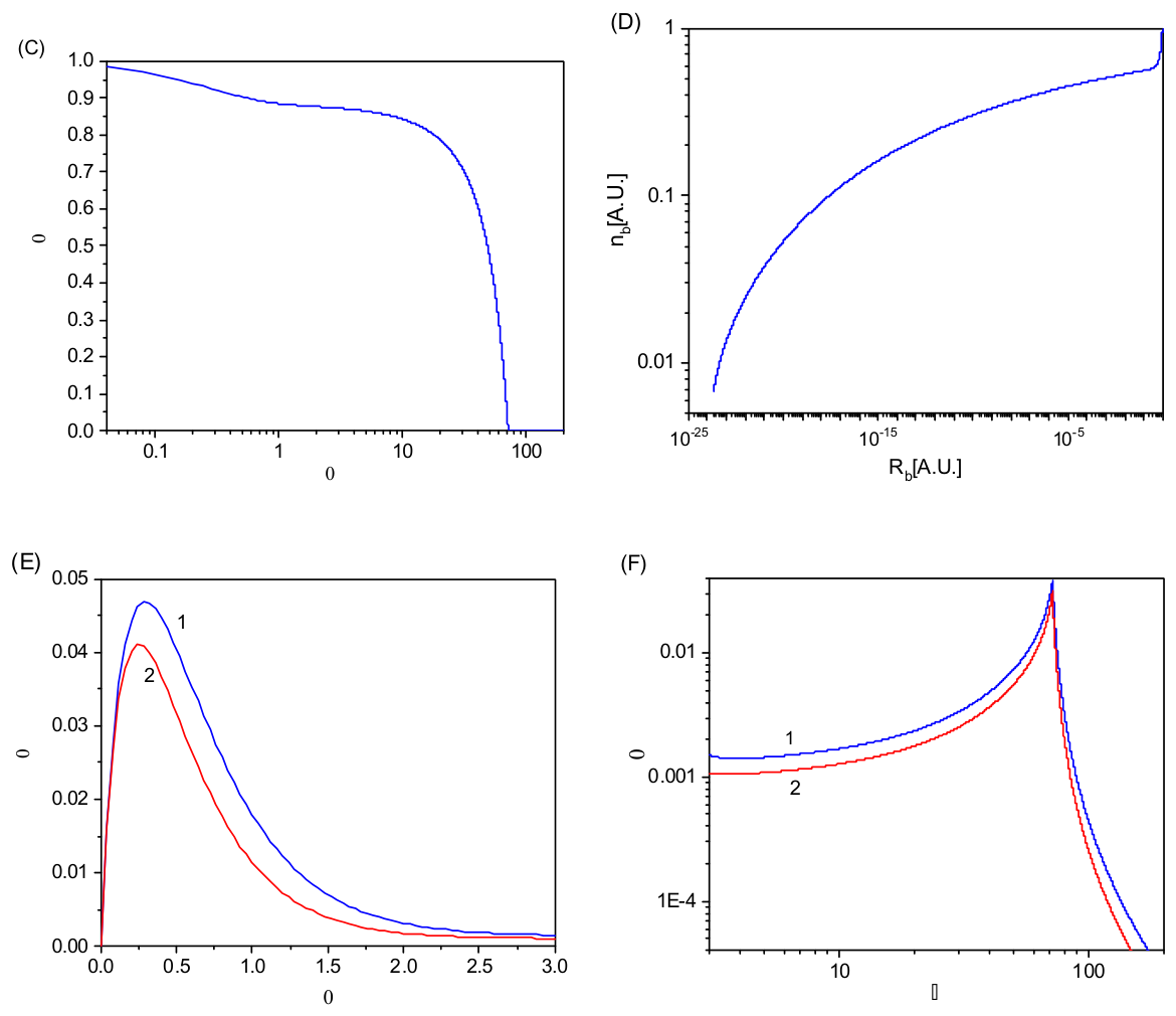
Figure 14.
Dependence of the ratio at time . (A) Dependence on , calculated using Eq. (48), with , , and . (B) Dependence on , calculated using Eq. (48), with , , and . (C) Dependence on , calculated using Eq. (48), with , , and . (D) Dependence on , calculated using Eq. (51), with , , and . For all calculations, and were assumed.
Figure 14.
Dependence of the ratio at time . (A) Dependence on , calculated using Eq. (48), with , , and . (B) Dependence on , calculated using Eq. (48), with , , and . (C) Dependence on , calculated using Eq. (48), with , , and . (D) Dependence on , calculated using Eq. (51), with , , and . For all calculations, and were assumed.

| 0 | 0.9 | 1 | 0 |
| 1 | 0.7 | 1.14 | 2.86 |
| 2 | 0.5 | 1.37 | 4.57 |
| 3 | 0.3 | 1.86 | 9.14 |
| 4 | 0.1 | 3.65 | 36/57 |
Disclaimer/Publisher’s Note: The statements, opinions and data contained in all publications are solely those of the individual author(s) and contributor(s) and not of MDPI and/or the editor(s). MDPI and/or the editor(s) disclaim responsibility for any injury to people or property resulting from any ideas, methods, instructions or products referred to in the content. |
© 2026 by the authors. Licensee MDPI, Basel, Switzerland. This article is an open access article distributed under the terms and conditions of the Creative Commons Attribution (CC BY) license (http://creativecommons.org/licenses/by/4.0/).
Copyright: This open access article is published under a Creative Commons CC BY 4.0 license, which permit the free download, distribution, and reuse, provided that the author and preprint are cited in any reuse.


